Article

Poor Visibility in Winter Due to Synergistic Effect Related to Fine Particulate Matter and Relative Humidity in the Taipei Metropolis, Taiwan

Centre for General Education, National Taipei University of Business, Taipei 10051, Taiwan
Atmosphere 2022, 13(2), 270; https://doi.org/10.3390/atmos13020270
Submission received: 23 December 2021 / Revised: 26 January 2022 / Accepted: 3 February 2022 / Published: 5 February 2022

Abstract

:
Visibility is important because it influences transportation safety. This study examined the relationships among sea–land breezes, relative humidity (RH), and the urban heat island (UHI) effect. The study also sought to understand how the synergistic effects of fine particulate matter (PM2.5) and RH influence visibility. Hourly meteorological, PM2.5 concentration, and visibility data from 2016 to 2019 were obtained from government-owned stations. This study used quadratic equations, exponential functions, and multi-regression models, along with a comparison test, to analyse the relationships between these variables. While sea breezes alone cannot explain the presence of PM2.5, UHI circulation coupled with sea breezes during winter can promote the accumulation of PM2.5. The synergistic effects of RH, PM2,5, and aerosol hygroscopicity exist in synoptic patterns type I and type III. PM2.5 was negatively correlated with visibility in the winter, when the RH was 67–95% and the continental cold high-pressure (CCHP) system was over the Asian continent (type I), or when the RH was 49–89% and the CCHP had moved eastward, with its centre located beyond 125° E (type III). The synergistic predictor variable PM2.5×RH was more important than PM2.5 and RH individually in explaining the variation in visibility.

1. Introduction

Visibility is closely related to air pollution [1,2,3,4], and its decrease has mainly been attributed to fine particulate matter (PM2.5) [5]. In some areas, owing to low air quality monitoring budgets, air quality is assessed by observing regional visibility. However, visibility is affected by many factors such as rainfall, fog, and haze. To avoid misjudging the air quality, it is important to identify the factors that influence visibility.
When rainfall and fog are absent, visibility can be reduced owing to absorption or scattering of light by particulate matter or gases. In this study, the daily mean concentration of NO2 was low in the Taipei metropolis; therefore, light absorption by gases was too low to be considered as a factor influencing visibility. Hence, this study focused on the relationship between visibility and PM2.5.
The effects of PM2.5 concentrations have a great impact on the health of the population. Many studies have shown a connection between PM2.5 and related diseases such as respiratory illnesses [6,7], cardiovascular illnesses [8,9], and diabetes [10]. Public health issues related to PM2.5 are an increasing concern worldwide.
PM2.5 concentrations are affected by sulphur dioxide and nitrogen dioxide emitted during the burning of fossil fuels and biomass [11], which can affect visibility. Several studies have discussed the relationship between PM2.5 concentration and visibility, which becomes complicated when weather conditions such as relative humidity (RH) are considered. For example, Zhou et al. [12] indicated that PM2.5 concentrations were significantly correlated with visibility in Beijing. Song et al. [13] indicated that during two haze events in Chengdu, China, between 23 December 2016 and 31 January 2017, visibility decreased as moisture absorption by aerosols increased along with increasing RH. Guan et al. [14] indicated that visibility can increase when the RH is less than 20% and decrease because of the synergistic effects of RH, sulphates, nitrates, and secondary organic carbon when the RH is greater than 60%. Wang et al. [15] indicated that PM2.5 concentrations can dominate the variation in visibility when the RH and PM2.5 concentrations are low, but visibility decreases drastically when the RH and PM2.5 concentrations are high.
Indirect reduction in visibility is affected by weather parameters. For example, the RH can influence PM2.5 size and composition, which can further influence the scattering and absorption of light by PM2.5. Sea and land breezes and urban heat islands (UHIs) are related to thermally driven circulation, and cooling disrupts circulation [16]. Sea and land breezes can influence the RH and increase or decrease PM2.5 concentration on land [17]. The UHI effect can influence the turbulence and RH, which can affect the PM2.5 concentration, composition, and size.
Several studies have found a relationship between visibility and weather conditions. Goyal et al. [18] indicated that visibility was negatively correlated with RH and positively correlated with daily maximum and minimum air temperatures and solar hours in Delhi, India. In a study conducted in 2013, Xue et al. [4] indicated that visibility decreased from 25 to 16 km when the weather conditions included low wind speed (WS), low air temperature, and high RH in Shanghai, China. Despite the decrease, however, the visibility was still considered good. Li et al. [19] analysed haze events in northern China from 1 December 2016 to 9 January 2017 and found that low visibility was associated with low WS from the south in the low troposphere. Furthermore, the minimum mean visibility was 3.4 km when the mean minimum WS was 0.05 m/s for the ten air pollution episodes. Shi et al. [3] indicated that a decrease in visibility was partly related to a decrease in WS in the low troposphere in the Beijing–Tianjin–Hebei region in China from 1961 to 2014, partly due to the significant slope of the mean WS at 10 m, which was −0.19 m/s/decade. Deng et al. [20] conducted a study from December 2016 to January 2017 and found that low visibility was related to low WS, high RH, low sunshine, high cloud cover, and weak East Asian monsoons. For example, after 1 January 2017, the minimum visibility was <1 km when the WS was <2 m/s and the RH was nearly saturated at the Fuyang station.
In northern Taiwan, the UHI effect can cause sea breezes to increase during the daytime, thus influencing the dispersion of air pollutants [21]. The weather conditions of the Taipei metropolis on Taiwan Island are highly dependent on the ocean. Unlike recent studies related to visibility in Taiwan addressing topics such as the trend in mean visibility [22], major species inducing poor visibility [23], and improvement of visibility forecasts [24], among others, the aim of this study was to answer two essential questions. First, what are the relationships among sea and land breezes, RH, and the UHI effect under the influence of the continental cold high-pressure system? Second, how does the synergistic effect of PM2.5 and RH influence the variation in visibility?

2. Materials and Methods
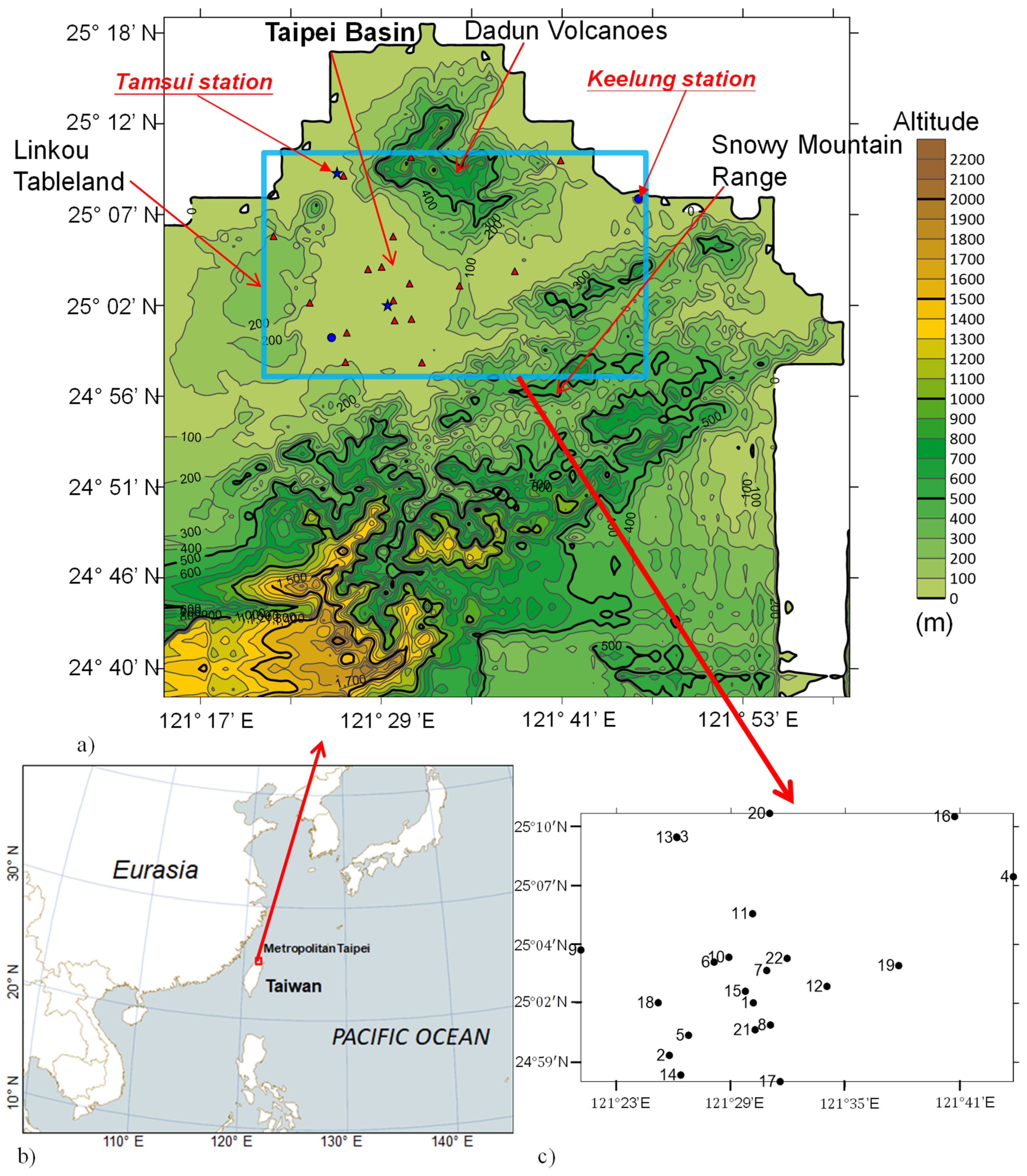
2.1. Study Area

The Taipei metropolis, with a population of 6.66 million [25], is the largest metropolitan area on Taiwan Island. Because the city is in a basin (Figure 1a), weather conditions and air quality are strongly influenced by topographical effects. In addition, the city is close to the East Sea, and therefore, sea–land breezes also affect the atmospheric environment. Thus, the metropolis is a suitable place to observe the relationship between visibility and PM2.5, as well as that between visibility and RH. In this study, the annual mean PM2.5 concentration at 17 stations in the Taipei metropolis from 2016 to 2019 was 15.3 ± 1.7 µg/m3, which is greater than the World Health Organization (WHO) guideline of 5 µg/m3 [26] and the Taiwan Environmental Protection Administration (EPA) guideline of 15 µg/m3 [27]. The 24 h mean PM2.5 concentration at the 17 stations in the Taipei metropolis in winter from 2016 to 2019 was 16.6 ± 8.9 µg/m3, which is greater than the WHO guideline of 15 µg/m3 [26] but smaller than the Taiwan EPA guideline of 35 µg/m3 [27].
Taiwan Island is located between the Eurasian continental plate and the Pacific Ocean (Figure 1b). On the island, the north-easterly monsoon dominates winter weather patterns, and the south-westerly monsoon dominates summer weather patterns. Usually, air pollutants in Taiwan originate from the Asian continent through long-range transport during the north-easterly monsoon [28,29,30]. The mean PM2.5 concentration in the Taipei metropolis in winter is greater than that in the summer [31]. Thus, this study focused on the winter period.

2.2. Observational Data

In this study, the winter season was defined as 1 October–30 April. The study period spanned the winter seasons from 2016 to 2019. Table 1 presents the geographical information for the data sites. Weather data such as the hourly air temperature (°C), dew air temperature (°C), RH (%), WS (m/s), rainfall (mm), visibility (km), and global solar radiation (GSR, kJ/m2) were obtained from the Central Weather Bureau (CWB) in Taiwan for the Taipei, Banqiao, Taisumi, and Keelung stations. According to the observation guidelines [32], the visibility (km) data at the CWB stations are observed manually ten times per day at 02:00, 05:00, 08:00, 09:00, 11:00, 14:00, 17:00, 20:00, 21:00, and 23:00 local standard time (LST). Other visibility (m) data were obtained from the Meteorological Terminal Aviation Routine Weather Report (METAR) from the station at the Songsang International Airport, which is located in the Taipei metropolis and administered by the Civil Aeronautics Administration of the Ministry of Transportation and Communications in Taiwan [33].
Hourly data on PM2.5 concentrations (μg/m3) at 17 air-quality monitoring stations in the Taipei metropolis have been offered by the Taiwan EPA since August 2005. Monitoring of PM2.5 data includes both manual and automatic monitoring. According to the Taiwan Air Quality Standard, manual monitoring is preferred. To maintain the consistency of PM2.5 data between manual and automatic monitoring, the national linear regression (relation) equation was used to calibrate the PM2.5 data from automatic monitoring from 1 January 2014 until 24 September 2019 [27,34]. To ensure efficient operation, manual monitoring instruments were scheduled for monthly and yearly calibrations, and automatic monitoring instruments were scheduled for weekly, biweekly, monthly, quarterly, half-yearly, and yearly calibrations (instrument features are described in detail in the Air Quality Annual Report) [27]. The stations and monitoring sites are shown in Figure 1a. To remove the effects of rainfall and fog on visibility, the analysed data points were removed if they met the following three criteria: the hourly air temperature was equal to the dew air temperature, the hourly RH was 100%, and the mean hourly rainfall was more than 0.1 mm.

2.3. Analysis Methodology

To understand the relationship between the mixing height and visibility, the Nozaki planetary boundary layer height (PBLH) [35] was utilised in this study, as shown in Equation (1) and Equation (2) to represent the mixing height of the Taipei metropolitan area. The parameters in the two equations were obtained from the Banqiao station (121°26′02″ E, 24°59′58″ N) using sounding data. The sounding data at the Banqiao station can be obtained only twice daily, at 08:00 and 20:00 LST, and thus it is not easy to observe the relationship between hourly PM2.5 concentrations and mixing height. Use of the PBLH can resolve the problem of insufficient data. This method has been applied in the field; for example, Du et al. [36] and Zheng and Zhang [37] conducted studies on the relationship between PBLH and air pollution.
PBLH = 121 6 ( 6 S ) ( T T d ) + 0.169 S ( W S h + 0.257 ) 12 f ln ( h / L )
f = 2 Ω sin θ  
S: stable parameters [38], refers to the stability classes suggested by Pasquill [39]; T-Td: the difference between surface air temperature and surface dew temperature; h: height of the sampling point above the ground (10 m in this study); WSh: mean WS at height (h) at the Banqiao station; f: earth rotation parameter; L: terrain rough length, according to the categories by Eagleson [40] (since the Banqiao station is within Taipei rather than in a rural area, the value of L was set as 2 m in this study); Ω: speed of Earth’s rotation, 0.0000727 rad/s; and θ: latitude of the station (24.9976° in this study).
When the UHI effect generates convergent air circulation, air pollutants accumulate in the hot centre. Li et al. [41] indicated that UHIs could worsen air quality and decrease the RH and visibility. RH and visibility were lower in the urban areas of Beijing, China, during summer than in the rural areas [42]. Three of the meteorological stations used in this study (Taipei, Banqiao, and Tamsui) offered high-quality data for calculating the UHI indices, unlike the automatic-monitoring meteorological sites. The mean air temperatures at the Taipei, Banqiao, and Tamsui meteorological stations in the winter seasons from 2016 to 2019 were 20.5 ± 4.6 °C, 20.2 ± 4.6 °C, and 19.6 ± 4.5 °C, respectively. As the Taipei station (121°30′24″ E, 25°02′23″ N) is located in downtown Taipei, it was set as an urban site, and because the Tamsui station (121°26′24″ E, 25°09′56″ N) is located in a rural setting at the edge of the Taipei Basin, it was set as a rural site. The altitudes of the Taipei and Tamsui stations are 5.3 m and 19 m, respectively. A value of 0.0891 °C was added to the air temperature at Tamsui to adjust for the effect of the environmental lapse rate, i.e., −6.5 °C/km in the U.S. Standard Atmosphere model at the altitude of the tropopause, 0–11 km [43]. In this study, the UHI index (°C) was defined as the air temperature at Taipei minus the air temperature at Tamsui using Equation (3) when the UHI effect was greater than 0.
UHI index = Tu − Tr
Tu: air temperature at Taipei station; Tr: air temperature at Tamsui station.
Relationships between visibility, PM2.5, and RH exist [13,15]. To homogenise the series of PM2.5, the independent variable (hourly RH, %) and dependent variable (hourly visibility, m) were fitted to a quadratic equation/exponential function model for several ranges of PM2.5, i.e., for every 5 μg/m3 of PM2.5 from the minimum to the maximum concentration. In each group, depending on the equation model that presented a greater R-square (R2) value, a pair of values a and b could be obtained from the quadratic equation (Equation (4)) or exponential function model (Equation (5)) (Table 2). The R2 value indicates the percentage of the variance of the visibility that can be explained by RH, which implies the performance of the explanatory power of the RH in the variation in visibility in the equation model. The above-mentioned method was applicable only if the PM2.5 concentrations were equal to, or greater than, 40 μg/m3.
Finally, the RH range could be obtained when the relationship between visibility and PM2.5 concentration in several groups of 5 μg/m3 was negative (Table 3). For example, Table 3 shows the negative relationship between visibility and PM2.5 concentration when the minimum RH, denoted x in Equations (4) and (5), was set to 49%, as shown in Figure 2b.
Finally, in this study, the relationships between visibility and PM2.5 concentrations in each group were examined using a quadratic equation model, represented by Equation (4).
y = a 1 x + a 2 x 2 + a 0 + ε
where y is the dependent variable, a 0 is a constant, a 1   and   a 2 are the coefficients of the predictor variables, ε is an error term, and x is the predictor variable.
y = a e b x
In Equation (5), y is the visibility (km) and x is PM2.5 (μg/m3).
Fisher’s least significant difference test was used to assess whether the differences in the values for the distinct groups were statistically significant [44]. This method was used to determine whether visibility and other parameters varied among the groups in the winter.
Multiple regression models were utilised to calculate visibility, assess whether a synergistic effect existed, and assess the extent of the contribution of the synergistic effect. Equation (6) represents the multiple linear regression model [45] used in this study.
y = β 1 x 1 + β 2 x 2 + β k x k   + β 0 + ε
where y is the dependent variable, β 0 is a constant, β 1 ,   β 2 , , β k are the coefficients of the predictor variables, ε is an error term, x 1 ,   x 2 , ,   x k are the predictor variables, and k is the number of predictor variables.
Equation (7) represents the standard multiple linear regression model used in this study. The coefficients of Equation (7) can be used to compare the important predictor variables because the predictor variables have been standardised.
Z y = β 1 Z 1 + β 2 Z 2 β k Z k + ε
where Z y is the standard dependent variable, β 1 ,   β 2 , , β k are the coefficients of the standard predictor variables, ε is an error term, Z 1 ,   Z 2 , ,   Z k are the standard predictor variables, and k is the number of standard predictor variables.
The forward stepwise multi-regression model with a screening procedure was utilised to select the most suitable model with reliable parameters related to visibility. The contributions of the parameters to explaining the variance in visibility were calculated stepwise. Two multi-regression models were used, one of which used parameters related to the synergistic effect. In addition, α-stay was set at 0.05. This variable was used in the model if the predictor variable was significant at an α-enter level of 0.05. To avoid highly inter-correlated predictor variables, the tolerance value of the predictor variables should be greater than 0.1. In addition, the Schwarz’s Bayesian information criterion (BIC) value for the model should be as low as possible to avoid a large difference from the unknown perfect model [46].

3. Results and Discussion

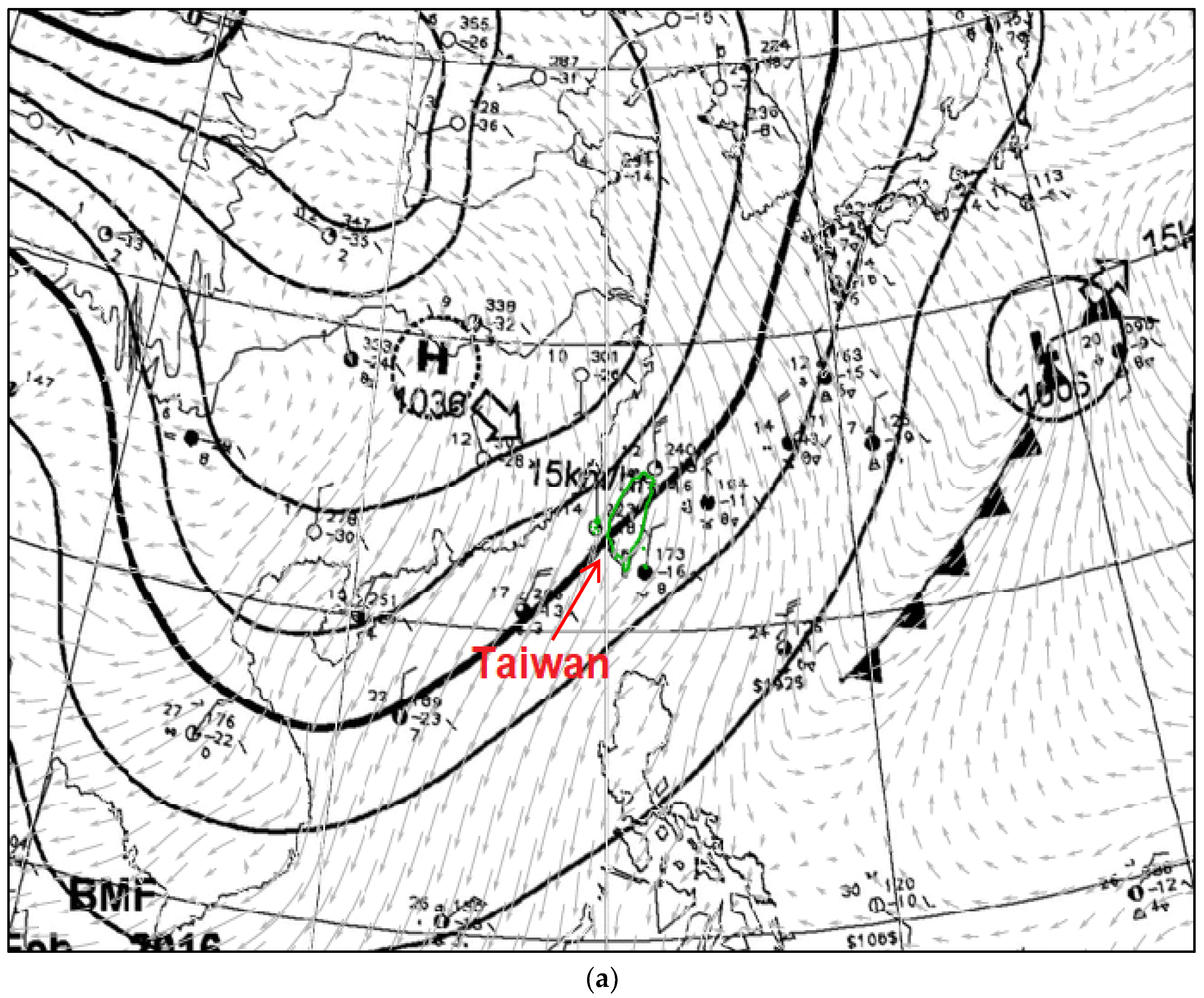
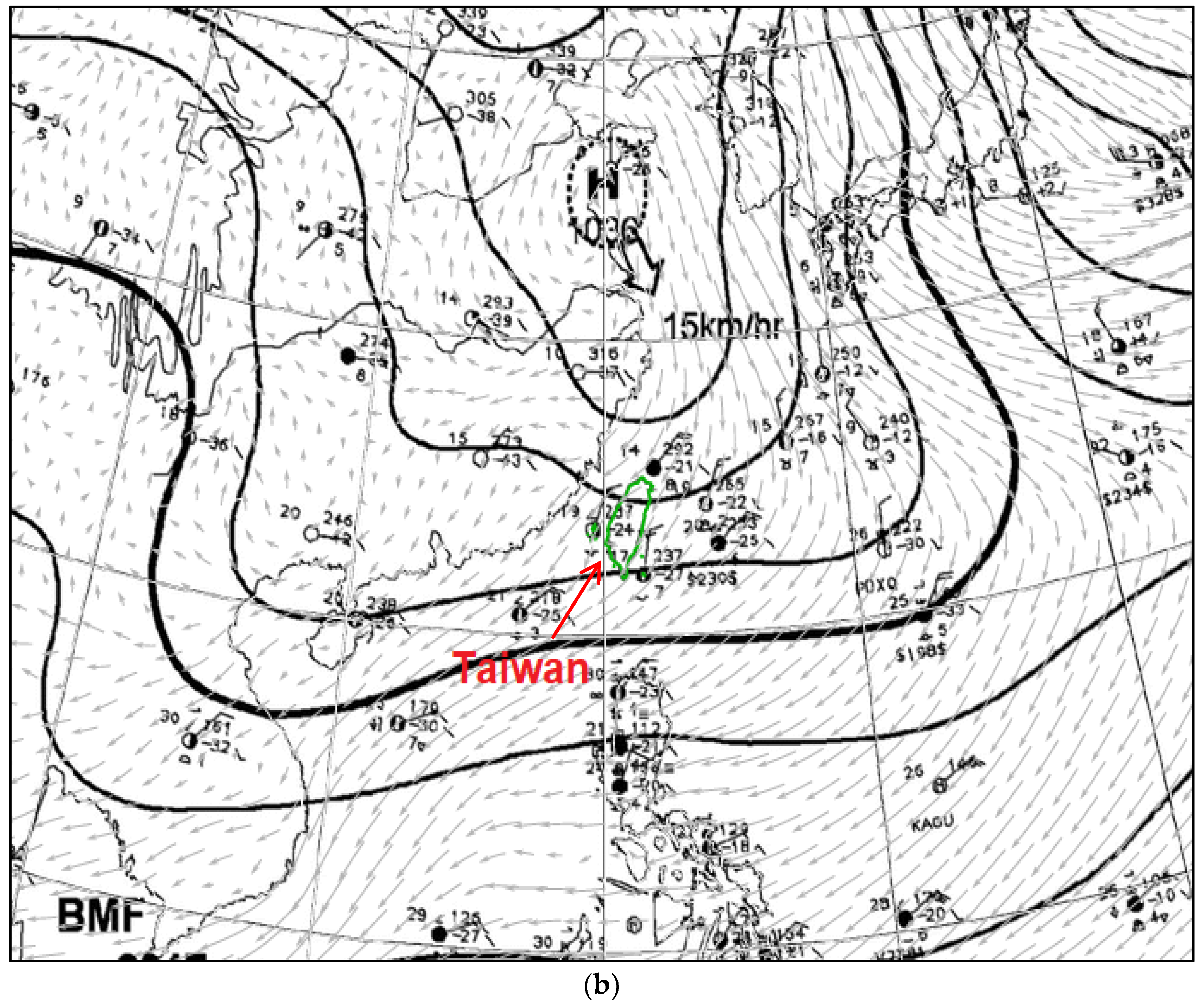
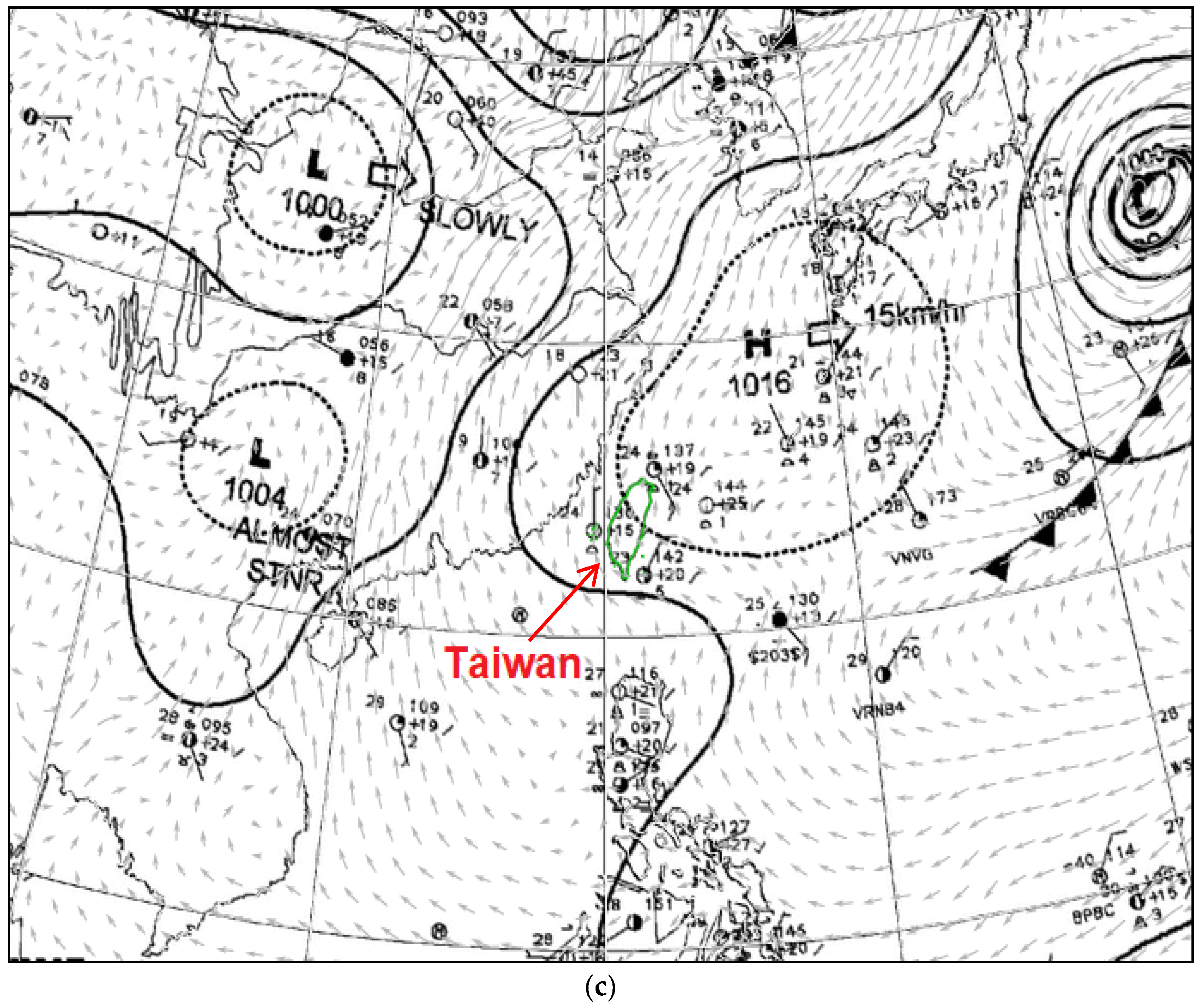
3.1. Synoptic Weather Patterns

Synoptic weather patterns can dominate the weather conditions of a region. For example, the weather in Taiwan is influenced by the north-easterly monsoon during the winter. Hsu and Cheng [47] suggested that high-pressure systems influence weather patterns in Taiwan during the winter in three ways: the influence of the high-pressure system on the Asian continent, that of the movement of the high-pressure system to the eastern coast of mainland China, and that of the movement of the high-pressure system away from the Asian continent. The highest PM2.5 concentrations and the lowest WS occurred during the third type of influence. In this study, the synoptic weather patterns dominating winter weather conditions in Taiwan were categorised into five types (Table 4). The main types directly related to the north-easterly monsoon system were type I, type II, and type III (Figure 3), accounting for 59.2% of the total.

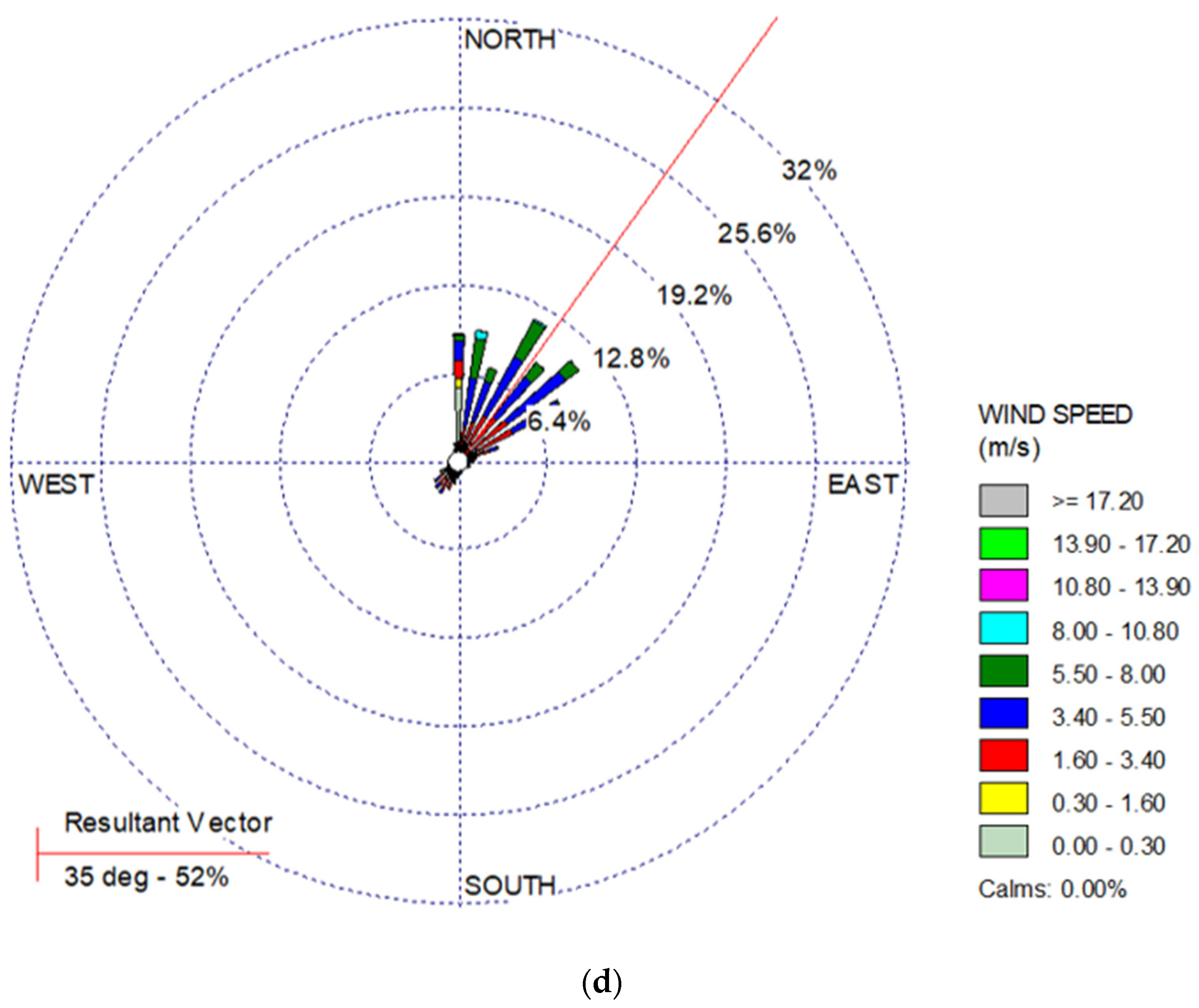
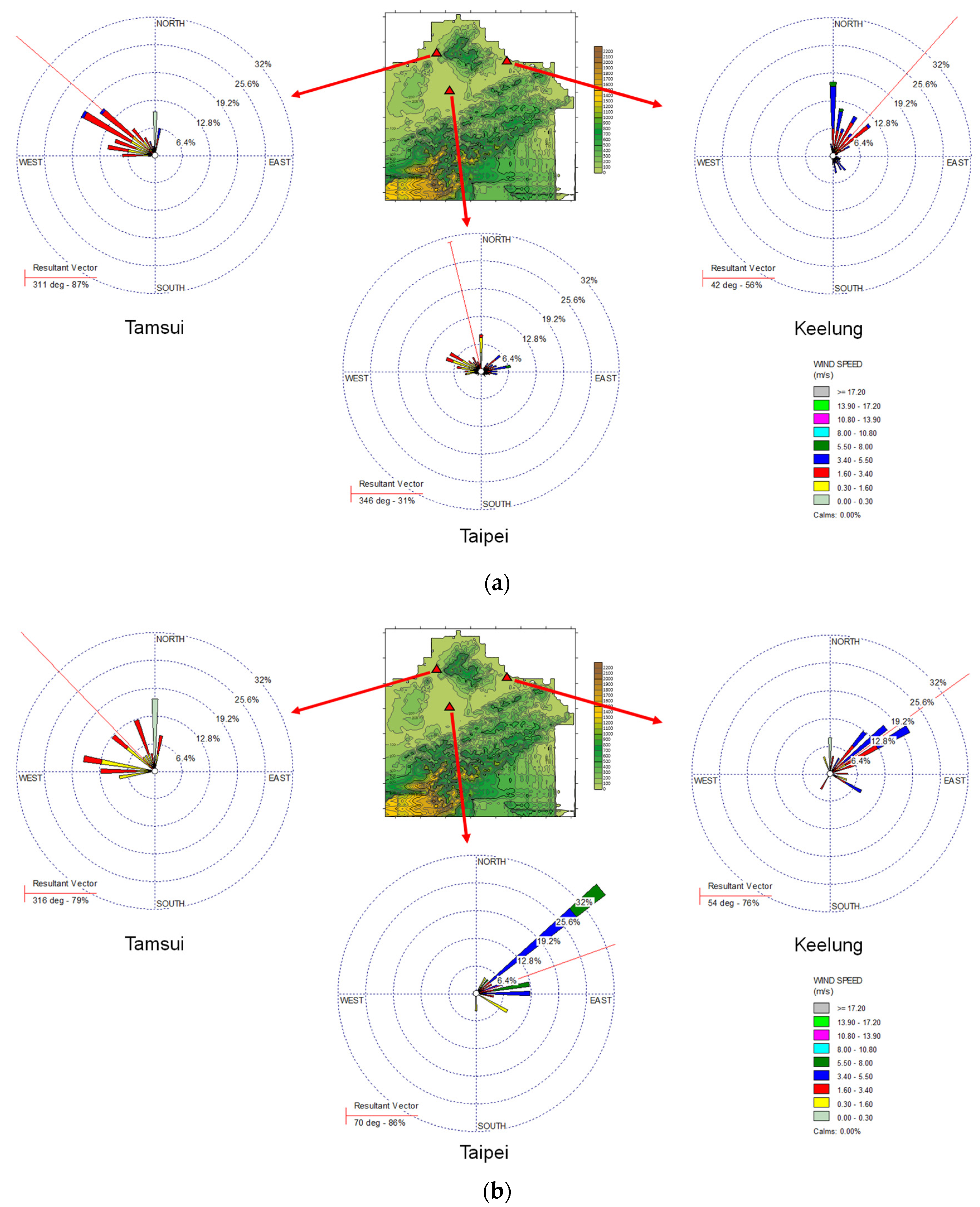
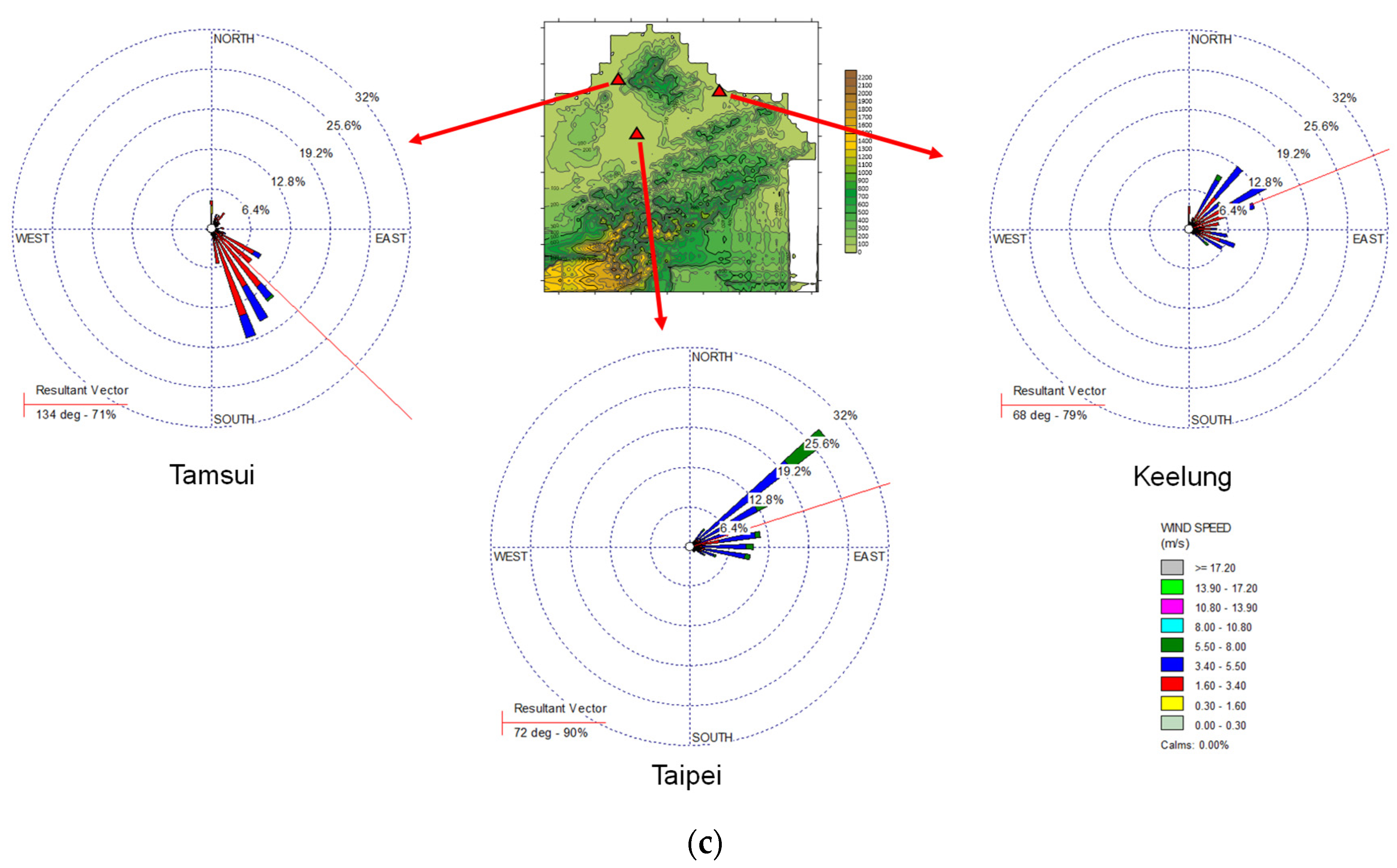
3.2. Sea and Land Breezes

Sea and land breezes are common phenomena in the Taipei metropolis [48]. The Tamsui station is located in one of the pathways of the north-westerly winds in the north-western Taipei Basin, and the Keelung station is located in the other pathway (Figure 1). Compared with the other meteorological stations, the Tamsui and Keelung stations are close to the sea and are in the upwind area of the basin in relation to the north-easterly monsoon. Therefore, in this study, they were selected as representative sites to study sea and land phenomena in the Taipei Basin. In this study, sea breezes in Tamsui and Keelung were defined by hourly wind directions between 258.75° and 11.25° and between 340° and 40°, respectively, mainly from the direction of the sea. In contrast, land breezes in Tamsui and Keelung were defined by hourly wind directions between 101.25° and 168.75° and between 120° and 270°, respectively, mainly originating inland. Figure 4a,c shows the relationship between WS and sea and land breezes during the winter at the Tamsui and Keelung sites. The results showed that sea breezes were prevalent mainly between 11:00 and 19:00 LST at the Tamsui site. During the day, the highest frequency of sea breezes was 72.1%. At night, the highest frequency of land breezes was 60.9%. The maximum mean WS was 2.37 m/s during the day, and the minimum was 1.37 m/s at night. At the Keelung site, the frequency of sea breezes was greater than that of land breezes, and the frequency of land breezes was relatively high between 0:00 and 8:00 LST. The maximum mean WS was 3.94 m/s during the day, and the minimum was 2.54 m/s at night. Figure 4b,d shows the frequency, direction, and intensity of the winds from 2016 to 2019 during the winter at the Tamsui and Keelung sites. The resultant vectors of the Tamsui and Keelung sites indicate that the mean wind direction was 50° and 30°, respectively. The frequency counts for the mean wind direction at the Tamsui and Keelung sites were 40% and 52%, respectively. The mean WSs of the Tamsui and Keelung sites were 1.72 m/s and 2.37 m/s, respectively.

3.3. Source of Moisture and Fine Particulate Matter
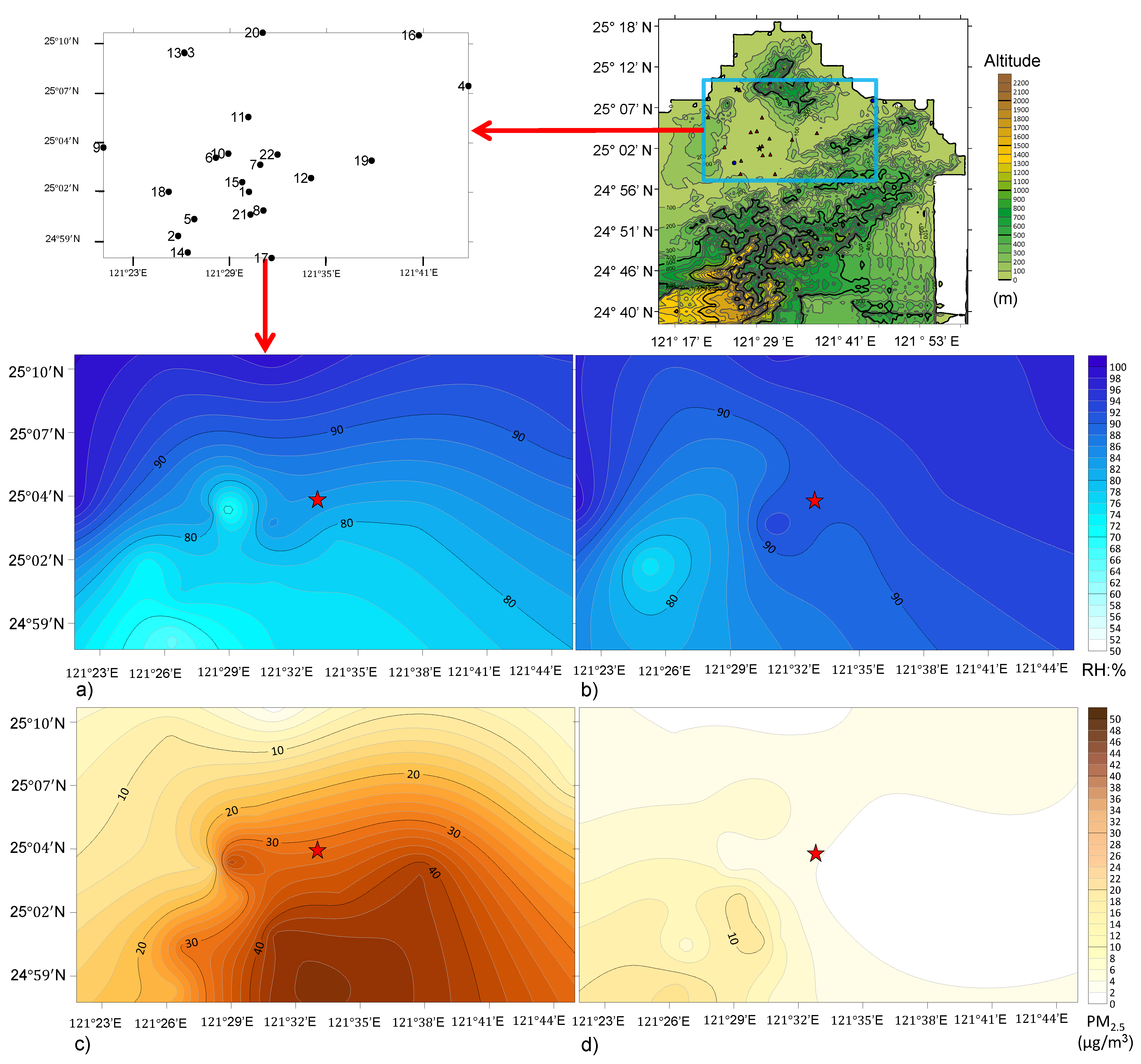
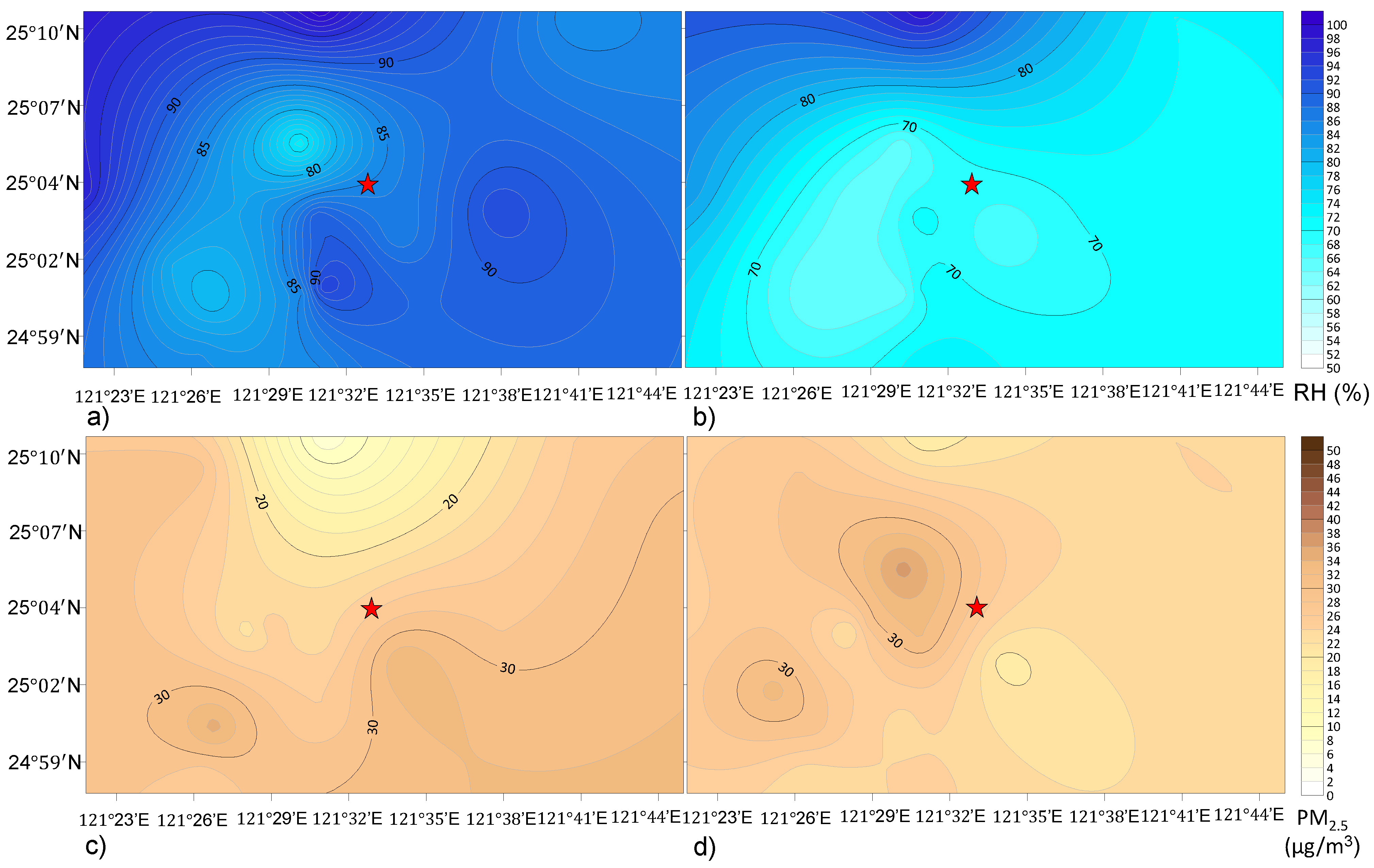
To determine whether a sea breeze influenced water pressure or PM2.5, whether UHI circulation coupled with a sea breeze influenced water pressure or PM2.5, and whether synoptic weather type III induced higher PM2.5 concentrations than type I, the synoptic weather patterns were divided, in this study, into four groups of weather conditions: group 1 (G1), group 2 (G2), group 3 (G3), and group 4 (G4) (Table 5). Each group was divided into subgroups A and B, which indicated obvious and non-obvious sea breezes, respectively, in the Taipei Basin. Synoptic weather pattern type II was not included among the analysed groups because the air flow brought by the continental cold high pressure (CCHP) could be wet, and its wind direction was not stable when the CCHP left the Asian continent heading seaward without going far offshore. Weather pattern type III could inhibit the phenomenon of the north-westerly, northern, and north-easterly winds interfering with the sea breeze. Table 5 lists the features of the main groups and subgroups. ‘Longitude < 121 ° E’ indicates that the CCHP was over the Asian continent. ‘Longitude > 125 ° E’ indicates that the CCHP had moved eastward, and its centre was located east of 125° E. ‘UHI > 0 °C’ indicates that the UHI phenomenon occurred in the Taipei metropolis. In G1, the CCHP was over the Asian continent, and the mean hourly air temperature of the Taipei metropolis was less than 20 °C, meaning that the north-easterly monsoon influenced the weather conditions in the Taipei metropolis. In addition, the UHI phenomenon was obvious. Compared to G1, the UHI phenomenon was not obvious in G3. In G2, the CCHP had moved eastward, its centre had moved past 125° E, and the mean hourly air temperature of the Taipei metropolis was greater than 20 °C, meaning that the east or south-easterly wind affected the weather conditions in the Taipei metropolis, as opposed to the north-easterly monsoon. In addition, the UHI phenomenon was obvious. In comparison to G2, the UHI phenomenon was not obvious in G4. In this study, to prevent rainfall from interfering with visibility data, the data collected when the rainfall was greater than 0.1 mm were excluded from analysis, and the corresponding weather was not classified in any of the groups. In addition, between 11:00 and 19:00 LST, the sea breeze phenomenon was obvious at the upwind sites, Tamsui and Keelung.

3.3.1. Moisture

Moisture is the relative humidity of the air, which is highly associated with air temperature. Excluding the influence of air temperature, this section used water pressure (hPa) as an index to estimate whether the north-easterly monsoon winds and the sea breeze were bringing moisture from the sea. Table 6 shows the differences in weather parameters between the groups shown in Table 5. Water pressure was not significantly greater in G2-A, compared to G4-A. The results show that the UHI circulation combined with sea breezes, but this did not notably increase the moisture brought to the Taipei Basin. Figure 5a,b shows that the magnitude of the resultant vector of 86% in the downwind area of the Taipei Basin in G4-A was greater than the 31% in G2-A. The results suggest that in synoptic weather type III, sea breeze phenomena without the UHI effect were more obvious than those with the UHI effect, meaning that the UHI effect might interrupt the inland propagation of sea breezes [49,50].
The water pressure was not significantly greater in G3-B (14.3 ± 2.6 hPa, p > 0.05) than in G4-B (19.2 ± 4.2 hPa). The water pressure was not greater in synoptic weather type I than in synoptic weather type III. The results suggest that during periods with no sea breezes, the north-easterly monsoon brings cold air instead of wet air to the Taipei Basin.
The water pressure was significantly greater in G3-A (15.3 ± 1.6 hPa, p < 0.05) than that in G3-B (14.3 ± 2.6 hPa). The water pressure in G4-A was significantly greater (20.5 ± 2.6 hPa, p < 0.05) than that in G4-B (19.2 ± 4.2 hPa). Figure 5b,c shows that the sea phenomena in G4-A were more obvious than those in G4-B. The results showed that in synoptic weather types I and III, sea breezes notably influenced moisture in the Taipei metropolis because none of the UHI effects interrupted the inland propagation of sea breezes. This suggests that the influence of sea breezes was obvious during the period with no UHI effect. In addition, the water pressure was greater in the sea breeze domain than in the non-sea breeze domain.

3.3.2. Fine Particulate Matter

Mean PM2.5 concentrations were greater in G3-B than in G3-A, and greater in G4-B than in G4-A. The results showed that in both synoptic weather types I and III, the influence of sea breezes on mean PM2.5 concentrations in the Taipei metropolis was not obvious. This indicates that the sea breezes did not carry PM2.5 from the sea to the Taipei Basin and did not contribute to the accumulation of PM2.5.
In synoptic weather pattern type III, the interruption of the north-westerly, northern, and north-easterly winds combined with sea breezes could be avoided. Mean PM2.5 concentrations in G2-A (25.4 ± 11.6 μg/m3, p < 0.05) were greater than that in G4-A (13.9 ± 7.4 μg/m3). The results showed that UHI circulation coupled with the sea breezes can contribute to the accumulation of PM2.5, although the sea breezes cannot carry PM2.5 to the Taipei Basin.
The mean PM2.5 concentrations in G4-B were similar to those in G3-B. The results showed that the mean PM2.5 concentrations in synoptic weather type III were similar to those in synoptic weather type I, suggesting that the north-easterly monsoon did not carry significantly more PM2.5 to the Taipei Basin in the G3-B weather situation than in the G4-B weather situation.
Mean PM2.5 concentrations in G4-B were similar to those in G2-B. The results showed that mean PM2.5 concentrations in situations affected by the UHI effect were similar to those present without the UHI effect. It seems that in synoptic weather type III, the UHI circulation alone does not contribute to the accumulation of PM2.5 in the Taipei metropolis. However, the comparison between G2-A and G4-A shows that UHI circulation coupled with sea breezes contributes to the accumulation of PM2.5 in the Taipei Basin.
Mean PM2.5 concentrations were significantly greater in G1-B (19.3 ± 12.4 μg/m3, p < 0.05) than in G3-B (13.5 ± 9.8 μg/m3). The results showed that in the same type I synoptic weather type, mean PM2.5 concentrations in situations affected by the UHI effect were greater than those in situations without the UHI effect. The UHI effect can contribute to the accumulation of PM2.5. However, the comparison between G2-B and G4-B shows that UHI circulation alone cannot contribute to the accumulation of PM2.5 in the Taipei Basin. It seems that in synoptic weather pattern type I, the UHI effect alone can contribute to the accumulation of PM2.5, but in synoptic weather pattern type III, only the UHI circulation coupled with sea breezes can contribute to the accumulation of PM2.5 in the Taipei Basin.

3.4. Visibility, RH, and Fine Particulate Matter

Visibility variation depends on RH and PM2.5 concentration [12]. For example, Table 6 shows that the mean visibility in the Taipei metropolis and at Songsang International Airport in G4-B was significantly lower than that in G4-A, although the mean PM2.5 concentrations were similar, because the RH was greater in G4-B. In addition, the mean visibility in the Taipei metropolis and at Songsang International Airport in G1-B was similar to that of G3-B, although the mean PM2.5 concentrations in G1-B were significantly greater than those in G3-B, because the mean RH was greater in G3-B.
This study utilised a linear equation, a quadratic equation, and an exponential function to represent the relationship between visibility and RH, rather than using only the equation model where the concentration of PM2.5 was controlled. The R2 of the quadratic equation was greater than that of the linear and exponential function equations. This indicates that the performance of the explanatory power of the PM2.5 concentrations in the variation of the visibility in the quadric equation model was better than that in the linear equation and exponential function models. Figure 2 shows the observed quadratic equation models that outline the relationships between visibility and mean PM2.5 concentrations in the Taipei metropolis when the RH was confined to specific ranges.
These results were different from those reported by Zhang et al. [51], who found that the relationship between visibility and PM2.5 concentrations could be represented as an exponential function, within a certain range of RH, in Ningbo, China. It seems that the relationships among PM2.5, visibility, and weather conditions vary with geographical region [23,24,52].
The results indicate that there is a negative relationship between visibility and PM2.5 concentration, but this relationship depends on the specific weather conditions (Table 7). Visibility was negatively correlated with the PM2.5 concentration when the synoptic weather pattern was type I and the RH was 67–95%, and when the synoptic weather pattern was type III and the RH was 49–89%.
Figure 2 shows the relationship between mean PM2.5 concentration (μg/m3) in the Taipei metropolis and the visibility (m) at Songsang International Airport. The results showed that PM2.5 concentrations were negatively correlated with visibility when the RH was confined within a certain range during the winter under synoptic weather patterns type I and type III. Additionally, the results showed that a higher RH was associated with lower visibility. Several previous studies support the results of this study. For example, Guan et al. [14] indicated that visibility was high when the RH was less than 20%, and that synergistic effects of RH and air pollutants occurred when the RH was greater than 60%. Unlike the findings of Guan et al. [14], the results of this study further found that when the mean hourly PM2.5 concentrations were greater than or equal to 5 μg/m3, the RH was 67–95%, and the synoptic weather pattern was type I in the winter, visibility decreased as the PM2.5 concentration increased. When the mean hourly PM2.5 concentrations were greater than or equal to 5 μg/m3, the RH was 49–89%, and the synoptic weather pattern was type III during the winter, visibility decreased as PM2.5 concentration increased. In the synoptic weather pattern type III, which created warmer conditions than type I, the range of RH over which visibility was negatively related to PM2.5 concentration was smaller. Additionally, the synergistic effects of RH and PM2.5 were also observed. For example, the PM2.5 concentrations were 40–45 μg/m3 under synoptic weather pattern type I; under these conditions, the visibility at the Songsang International Airport was 8203.6 m when the RH was 67% and 5543.2 m when the RH was 95%. Singh et al. [52] found that visibility was related to RH, as aerosol hygroscopicity resulted in particulate scattering of solar radiation. Song et al. [13] found that rapid hygroscopic growth of aerosols degraded visibility as the RH increased. Figure 2 shows that the aerosol hygroscopicity effect might be prominent.

3.5. Contribution of Synergistic Effect

The forward stepwise multiple regression model was utilised to estimate the contributions of the parameters and test whether the synergistic effect affected the variation in visibility in the winter (Table 8). Model 1 shows the parameters without synergistic effects. Model 2 shows that the parameter PM2.5 × RH has a synergistic effect. The results showed that the most important variable of the final standard multiple linear regression model (Model 1) was PM2.5, which explained 31.1% of the variation in visibility. These results are similar to the findings of Kuo et al. [23], which suggested that PM2.5 explained 48.6% and 58.1% of the variation in visibility in the Taichung and Wuchi areas of Taiwan, respectively. Furthermore, Kuo et al. [23] also discovered that WS was an important contributing factor for explaining variations in visibility, with a 20.4% contribution. However, in this study, WS only presented 2.4% and 0.5% contributions to the variations in visibility in Models 1 and 2, respectively. Unlike previous studies, this study further considered the synergistic effects of multiple regression models. The most important variable of the final standard multiple linear regression model (Model 2) was PM2.5 × RH (R2 = 0.395). The contribution of the synergistic parameter in Model 2 was greater than the individual contributions of the parameters PM2.5 and RH in Model 1 with R2 values of 0.311 and 0.184, respectively. This indicates that visibility was highly correlated with PM2.5 coupled with RH.

3.6. Case Studies

Two cases showed a synergistic effect between PM2.5 and RH. To avoid interference from other factors, the two cases were prepared according to the same weather conditions where the synoptic weather pattern was type I and the mean rainfall amount was lower than 0.1 mm.
For the first case, Figure 6a,c shows the distribution of RH and PM2.5 concentrations, respectively, at 14:00 LST on 5 January 2019. At this time, the mean hourly PM2.5 concentration in the Taipei metropolis was 25.9 µg/m3, and the mean RH was 86.3%. Figure 6b,d shows the distribution of RH and PM2.5 concentrations, respectively, at 14:00 LST on 22 February 2019. The mean hourly PM2.5 concentration in the Taipei metropolis was 5.1 µg/m3, and the mean RH was 86.3%. The visibility at Songsang International Airport at 14:00 LST on 5 January 2019 was only 6000 m, whereas it was 10,000 m at 14:00 LST on 22 February 2019. The mean visibility in the Taipei metropolis on the earlier date was only 5 km, less than the 12 km observed on the later date. As expected, the higher mean hourly PM2.5 concentrations induced lower visibility when the RH was constant. This implies that if the RH is constant, visibility cannot completely account for PM2.5 concentrations.
In contrast, in the second case, Figure 7a,c shows the distribution of RH and PM2.5 concentration, respectively, at 14:00 LST on 24 February 2016 in the Taipei metropolis. The mean hourly PM2.5 concentration was 25.9 µg/m3, and the mean RH was 84.7%. Figure 7b,d shows the distribution of RH and PM2.5 concentration, respectively, at 14:00 LST on 14 March 2016. At this time, the mean hourly PM2.5 concentration was 25.9 µg/m3; however, the mean hourly RH was 68%. The visibility at Songsang International Airport at 14:00 LST on 24 February 2016 was only 5000 m, lower than the 12,000 m observed at 14:00 LST on 14 March 2016, although the mean hourly PM2.5 concentrations in the Taipei metropolis were the same. The mean visibility in the Taipei metropolis on the earlier date was only 6 km, less than the 10 km observed on the later date. The results suggest that the synergistic effect of high RH decreased visibility on the earlier date.

4. Conclusions

Unlike the sites in previous studies, the Taipei metropolis with a basin terrain located near the sea is an ideal setting for analysing the relationships among visibility, PM2.5, RH, and UHI. This study categorised three main types of synoptic weather patterns during the winter: the CCHP was over the Asian continent (type I); the CCHP had left the Asian continent, but its centre was not beyond 125° E (type II); and the CCHP had moved eastward, with its centre located beyond 125° E (type III). This study found that the relationships between sea breeze, UHI, and RH varied by synoptic weather pattern. The RH of the air is a climatic variable that is highly dependent on air temperature; the RH is negatively related to air temperature when moisture is constant. Thus, the relationship between visibility and PM2.5 varies by climatic region. The main findings were as follows:
(a)
The sea breeze phenomena without the UHI effect were more obvious than those with the UHI effect. The influence of synoptic weather pattern type I on moisture was not obvious during the period with no UHI effect and sea breezes, even during the winter, and the water pressure was greater when the sea breezes were prominent.
(b)
The UHI circulation alone cannot contribute to the accumulation of PM2.5 in the Taipei metropolis. UHI circulation coupled with sea breezes can contribute to the accumulation of PM2.5, although sea breezes cannot carry PM2.5.
(c)
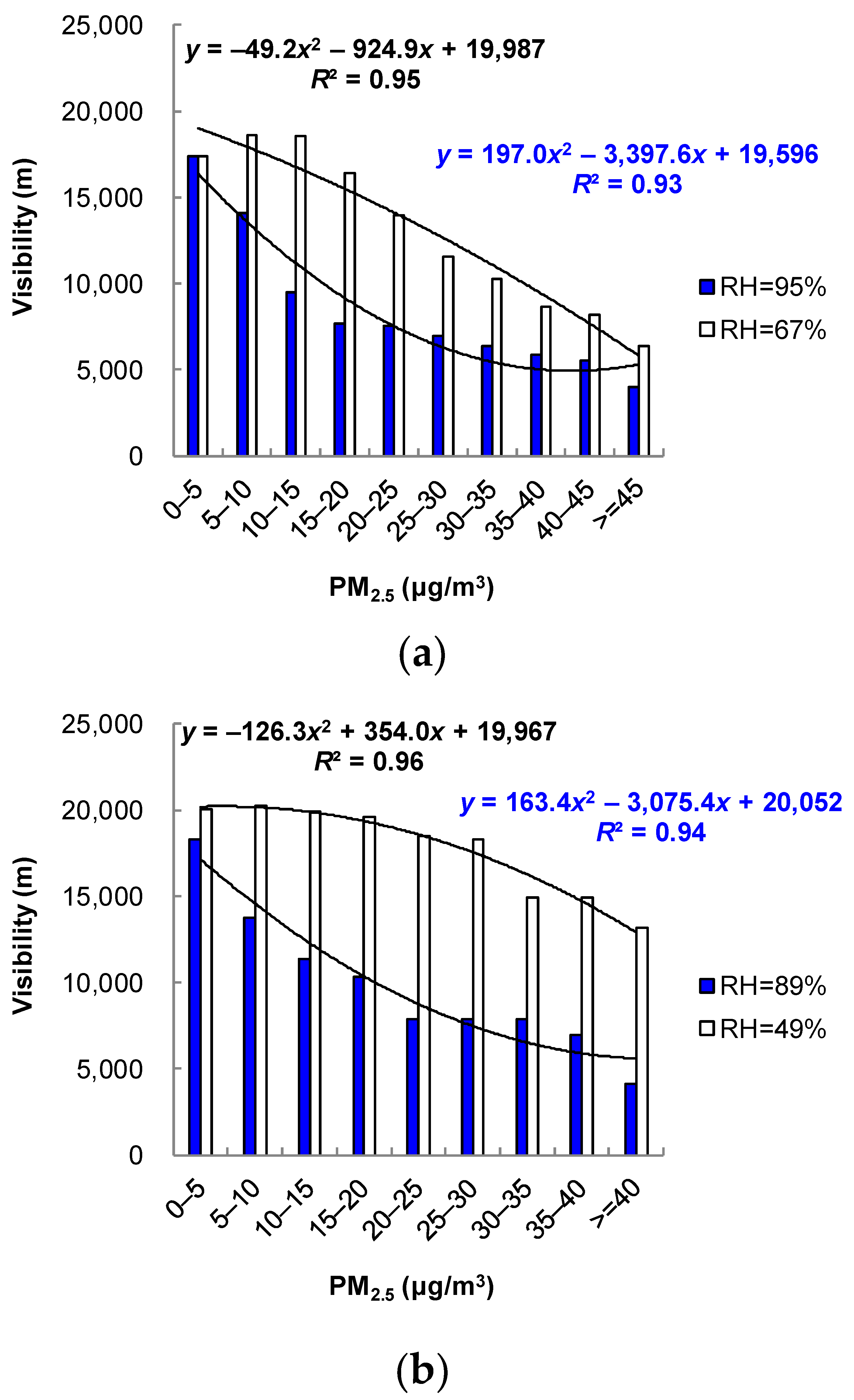
Quadratic equation models represented the relationship between the visibility and mean PM2.5 concentrations in the Taipei metropolis, as RH was confined to specific ranges. The PM2.5 concentrations, when greater than or equal to 5 μg/m3, were negatively correlated with visibility during the winter when the RH was 67–95% under synoptic weather pattern type I and when the RH was 49–89% under synoptic weather pattern type III. The synergistic effects of RH, PM2.5, and aerosol hygroscopicity were observed in both synoptic weather patterns.
(d)
Comparisons between groups of distinct weather conditions, the quadratic equation models, and two case studies indicated the predictor variables of the synergistic effects. PM2.5 × RH was prominent in explaining the variation in visibility in the Taipei metropolis.
A severe decrease in visibility can cause car accidents on highways and threaten the safe take-off and landing of airplanes in airports. Governmental authorities should consider UHI-effect reduction strategies such as improvement of urban ecological land [53] and should be concerned about low visibility in winter, particularly when PM2.5 concentrations and RH are high under synoptic weather pattern type I.

Funding

This research was funded by the Taiwan Ministry of Science and Technology, grant number MOST 109-2111-M-141-001.

Data Availability Statement

The air pollutant concentration data are available at the Taiwan Environmental Protection Administration [https://airtw.epa.gov.tw/CHT/Query/His_Data.aspx] (accessed on 22 November 2021). The meteorological data are available at the Data Bank for Atmospheric and Hydrological Research in the Department of Atmospheric Science, Chinese Culture University [https://dbar.pccu.edu.tw/Default.aspx] (accessed on 22 November 2021).

Acknowledgments

The authors are grateful to the Taiwan Central Weather Bureau (CWB) and the Environmental Protection Administration for providing meteorological and air pollutant concentration data. The authors are grateful to the Central Geological Survey at the Ministry of Economic Affairs for providing the digital terrain model data. The authors also thank the Data Bank for Atmospheric and Hydrological Research in the Department of Atmospheric Science at the Chinese Culture University for providing the meteorological data owned by the CWB.

Conflicts of Interest

The authors declare no conflict of interest.

References

  1. Huang, W.; Cai, L.; Dang, H.; Jiao, Z.; Fan, H.; Cheng, F. Review on formation mechanism analysis method and control strategy of urban haze in China. Chin. J. Chem. Eng. 2018, 27, 1572–1577. [Google Scholar] [CrossRef]
  2. Kim, J.-S.; Zhou, W.; Cheung, H.N.; Chow, C.H. Variability and risk analysis of Hong Kong air quality based on Monsoon and El Niño conditions. Adv. Atmos. Sci. 2013, 30, 280–290. [Google Scholar] [CrossRef]
  3. Shi, P.; Zhang, G.; Kong, F.; Chen, D.; Azorin-Molina, C.; Guijarro, J.A. Variability of winter haze over the Beijing-Tianjin-Hebei region tied to wind speed in the lower troposphere and particulate sources. Atmos. Res. 2018, 215, 1–11. [Google Scholar] [CrossRef]
  4. Xue, D.; Li, C.; Liu, Q. Visibility characteristics and the impacts of air pollutants and meteorological conditions over Shanghai, China. Environ. Monit. Assess. 2015, 363, 1. [Google Scholar] [CrossRef] [PubMed]
  5. Hyslop, N.P. Impaired visibility: The air pollution people see. Atmos. Environ. 2009, 43, 182–195. [Google Scholar] [CrossRef]
  6. Xing, Y.-F.; Xu, Y.-H.; Shi, M.-H.; Lian, Y.-X. The impact of PM2.5 on the human respiratory system. J. Thorac. Dis. 2016, 8, E69–E74. [Google Scholar] [CrossRef]
  7. Ratajczak, A.; Badyda, A.; Czechowski, P.; Czarnecki, A.; Dubrawski, M.; Feleszko, W. Air Pollution Increases the Incidence of Upper Respiratory Tract Symptoms among Polish Children. J. Clin. Med. 2021, 10, 2150. [Google Scholar] [CrossRef]
  8. Du, Y.; Xu, X.; Chu, M.; Guo, Y.; Wang, J. Air particulate matter and cardiovascular disease: The epidemiological, biomedical and clinical evidence. J. Thorac. Dis. 2016, 8, E8–E19. [Google Scholar] [CrossRef]
  9. Jalali, S.; Karbakhsh, M.; Momeni, M.; Taheri, M.; Amini, S.; Mansourian, M.; Sarrafzadegan, N. Long-term exposure to PM2.5 and cardiovascular disease incidence and mortality in an Eastern Mediterranean country: Findings based on a 15-year cohort study. Environ. Health 2021, 20, 112. [Google Scholar] [CrossRef]
  10. Chilian-Herrera, O.L.; Tamayo-Ortiz, M.; Texcalac-Sangrador, J.L.; Rothenberg, S.J.; López-Ridaura, R.; Romero-Martínez, M.; Wright, R.O.; Just, A.C.; Kloog, I.; Bautista-Arredondo, L.F.; et al. PM2.5 exposure as a risk factor for type 2 diabetes mellitus in the Mexico City metropolitan area. BMC Public Health 2021, 21, 2087. [Google Scholar] [CrossRef]
  11. Zhao, H.; Ma, Y.; Wang, Y.; Wang, H.; Sheng, Z.; Gui, K.; Zheng, Y.; Zhang, X.; Che, H. Aerosol and gaseous pollutant characteristics during the heating season (winter–spring transition) in the Harbin-Changchun megalopolis, northeastern China. J. Atmos. Sol.-Terr. Phys. 2019, 188, 26–43. [Google Scholar] [CrossRef]
  12. Zhou, Y.; Cheng, S.; Chen, D.; Lang, J.; Wang, G.; Xu, T.; Wang, X.; Yao, S. Temporal and Spatial Characteristics of Ambient Air Quality in Beijing, China. Aerosol Air Qual. Res. 2015, 15, 1868–1880. [Google Scholar] [CrossRef] [Green Version]
  13. Song, M.; Liu, X.; Tan, Q.; Feng, M.; Qu, Y.; An, J.; Zhang, Y. Characteristics and formation mechanism of persistent extreme haze pollution events in Chengdu, southwestern China. Environ. Pollut. 2019, 251, 1–12. [Google Scholar] [CrossRef] [PubMed]
  14. Guan, L.; Liang, Y.; Tian, Y.; Yang, Z.; Sun, Y.; Feng, Y. Quantitatively analyzing effects of meteorology and PM2.5 sources on low visual distance. Sci. Total Environ. 2018, 659, 764–772. [Google Scholar] [CrossRef]
  15. Wang, X.; Zhang, R.; Yu, W. The Effects of PM 2.5 Concentrations and Relative Humidity on Atmospheric Visibility in Beijing. J. Geophys. Res. Atmos. 2019, 124, 2235–2259. [Google Scholar] [CrossRef]
  16. Ribeiro, F.N.; Oliveira, A.; Soares, J.; de Miranda, R.M.; Barlage, M.; Chen, F. Effect of sea breeze propagation on the urban boundary layer of the metropolitan region of Sao Paulo, Brazil. Atmos. Res. 2018, 214, 174–188. [Google Scholar] [CrossRef]
  17. Tsai, H.-H.; Yuan, C.-S.; Hung, C.-H.; Lin, C.; Lin, Y.-C. Influence of Sea-Land Breezes on the Tempospatial Distribution of Atmospheric Aerosols over Coastal Region. J. Air Waste Manag. Assoc. 2011, 61, 358–376. [Google Scholar] [CrossRef] [Green Version]
  18. Goyal, P.; Kumar, A.; Mishra, D. The Impact of Air Pollutants and Meteorological Variables on Visibility in Delhi. Environ. Model. Assess. 2013, 19, 127–138. [Google Scholar] [CrossRef]
  19. Li, X.; Gao, Z.; Li, Y.; Gao, C.Y.; Ren, J.; Zhang, X. Meteorological conditions for severe foggy haze episodes over north China in 2016–2017 winter. Atmos. Environ. 2018, 199, 284–298. [Google Scholar] [CrossRef]
  20. Deng, X.; Cao, W.; Huo, Y.; Yang, G.; Yu, C.; He, D.; Deng, W.; Fu, W.; Ding, H.; Zhai, J.; et al. Meteorological conditions during a severe, prolonged regional heavy air pollution episode in eastern China from December 2016 to January 2017. Arch. Meteorol. Geophys. Bioclimatol. Ser. B 2018, 135, 1105–1122. [Google Scholar] [CrossRef]
  21. Lin, C.-Y.; Chen, F.; Huang, J.-C.; Chen, W.-C.; Liou, Y.-A.; Liu, S.-C. Urban heat island effect and its impact on boundary layer development and land–sea circulation over northern Taiwan. Atmos. Environ. 2008, 42, 5635–5649. [Google Scholar] [CrossRef]
  22. Maurer, M.; Klemm, O.; Lokys, H.L.; Lin, N.-H. Trends of Fog and Visibility in Taiwan: Climate Change or Air Quality Improvement? Aerosol Air Qual. Res. 2019, 19, 896–910. [Google Scholar] [CrossRef] [Green Version]
  23. Kuo, C.-Y.; Cheng, F.-C.; Chang, S.-Y.; Lin, C.Y.; Chou, C.C.; Chou, C.-H.; Lin, Y.-R. Analysis of the major factors affecting the visibility degradation in two stations. J. Air Waste Manag. Assoc. 2013, 63, 433–441. [Google Scholar] [CrossRef] [PubMed] [Green Version]
  24. Lin, J.C.-H.; Tai, J.-H.; Feng, C.-H.; Lin, D.-E. Towards Improving Visibility Forecasts in Taiwan: A Statistical Approach. Terr. Atmos. Ocean. Sci. 2010, 21, 359. [Google Scholar] [CrossRef] [Green Version]
  25. Department of Statistics. Ministry of the Interior. Available online: http://statis.moi.gov.tw/micst/stmain.jsp?sys=100 (accessed on 27 January 2021).
  26. World Health Organization (WHO). WHO Global Air Quality Guidelines. Particulate Matter (PM2.5 and PM10), Ozone, Nitrogen Dioxide, Sulfur Dioxide and Carbon Monoxide; WHO: Geneva, Switzerland, 2021. [Google Scholar]
  27. Environmental Protection Administration (EPA). Air Quality Annual Report of Taiwan; EPA: Taipei, Taiwan, 2018.
  28. Lai, I.-C.; Brimblecombe, P. Long-range Transport of Air Pollutants to Taiwan during the COVID-19 Lockdown in Hubei Province. Aerosol Air Qual. Res. 2021, 21, 200392. [Google Scholar] [CrossRef]
  29. Lin, C.-Y.; Wang, Z.; Chen, W.-N.; Chang, S.-Y.; Chou, C.C.K.; Sugimoto, N.; Zhao, X. Long-range transport of Asian dust and air pollutants to Taiwan: Observed evidence and model simulation. Atmos. Chem. Phys. 2007, 7, 423–434. [Google Scholar] [CrossRef] [Green Version]
  30. Wu, P.-C.; Huang, K.-F. Tracing local sources and long-range transport of PM10 in central Taiwan by using chemical characteristics and Pb isotope ratios. Sci. Rep. 2021, 11, 7593. [Google Scholar] [CrossRef]
  31. Lai, L.-W. Fine particulate matter events associated with synoptic weather patterns, long-range transport paths and mixing height in the Taipei Basin, Taiwan. Atmos. Environ. 2015, 113, 50–62. [Google Scholar] [CrossRef]
  32. Central Weather Bureau (CWB). Regulations for Ground Meteorological Observation; CWB: Taipei, Taiwan, 2004.
  33. Civil Aeronautics Administration; Ministry of Transportation and Communications (CAA, MOTC). Aeronautical Meteorology Norms; College Art Association, Ministry of Transporation and Communications ROC: Taipei, Taiwan, 2021.
  34. Environmental Protection Administration (EPA). Manual Monitoring of Fine Particulate Matter. Available online: https://airtw.epa.gov.tw/ENG/EnvMonitoring/Central/spm.aspx (accessed on 22 November 2021).
  35. Nozaki, K.Y. Mixing Depths Model Using Hourly Surface Observations; Report 7053; USAF Environmental Technical Applications Center: Patrick Space Force Base, FL, USA, 1973. [Google Scholar]
  36. Du, C.; Liu, S.; Yu, X.; Li, X.; Chen, C.; Peng, Y.; Dong, Y.; Dong, Z.; Wang, F. Urban Boundary Layer Height Characteristics and Relationship with Particulate Matter Mass Concentrations in Xi’an, Central China. Aerosol Air Qual. Res. 2013, 13, 1598–1607. [Google Scholar] [CrossRef]
  37. Zeng, S.; Zhang, Y. The Effect of Meteorological Elements on Continuing Heavy Air Pollution: A Case Study in the Chengdu Area during the 2014 Spring Festival. Atmosphere 2017, 8, 71. [Google Scholar] [CrossRef] [Green Version]
  38. NOAA Air Resources Laboratory. Pasquill Stability Classes 1961. Available online: https://www.ready.noaa.gov/READYpgclass.php (accessed on 27 September 2021).
  39. Pasquill, F.; Smith, F. The physical and meteorological basis for the estimation of the dispersion of windborne material. In Proceedings of the Second International Clean Air Congress, Washington, DC, USA, 6–11 December 1970; Academic Press Inc.: New York, NY, USA, 1971; pp. 1067–1072. [Google Scholar] [CrossRef]
  40. Eagleson, P.S. Dynamic Hydrology; McGraw-Hill: New York, NY, USA, 1970. [Google Scholar]
  41. Li, Z.-H.; Yang, J.; Shi, C.-E.; Pu, M.-J. Urbanization Effects on Fog in China: Field Research and Modeling. Pure Appl. Geophys. 2011, 169, 927–939. [Google Scholar] [CrossRef]
  42. Hu, F.; Liu, X.-M.; Li, L.; Wang, Y. Summer Urban Climate Trends and Environmental Effect in the Beijing Area. Chin. J. Geophys. 2006, 49, 617–626. [Google Scholar] [CrossRef]
  43. American Meteorological Society (AMS). Standard Atmosphere. 2012. Available online: https://glossary.ametsoc.org/wiki/Standard_atmosphere (accessed on 29 September 2021).
  44. Systat. SYSTAT® 12 Getting Started; Systat Software, Incorp.: San Jose, CA, USA, 2007. [Google Scholar]
  45. Chernick, M.; Bowerman, B.L.; O’Connell, R.T. Forecasting and Time Series: An Applied Approach. Am. Stat. 1994, 48, 347. [Google Scholar] [CrossRef]
  46. Systat. Systat. Statistics-II; Systat Software, Incorp.: San Jose, CA, USA, 2007. [Google Scholar]
  47. Hsu, C.-H.; Cheng, F.-Y. Synoptic Weather Patterns and Associated Air Pollution in Taiwan. Aerosol Air Qual. Res. 2019, 19, 1139–1151. [Google Scholar] [CrossRef] [Green Version]
  48. Chen, T.-C.; Yen, M.-C.; Tsay, J.-D.; Liao, C.-C.; Takle, E.S. Impact of Afternoon Thunderstorms on the Land–Sea Breeze in the Taipei Basin during Summer: An Experiment. J. Appl. Meteorol. Clim. 2014, 53, 1714–1738. [Google Scholar] [CrossRef]
  49. You, C.; Fung, J.C.-H.; Tse, W.P. Response of the Sea Breeze to Urbanization in the Pearl River Delta Region. J. Appl. Meteorol. Clim. 2019, 58, 1449–1463. [Google Scholar] [CrossRef]
  50. Kang, Y.-H.; Song, S.-K.; Hwang, M.-K.; Jeong, J.-H.; Kim, Y.-K. Impacts of Detailed Land-Use Types and Urban Heat in an Urban Canopy Model on Local Meteorology and Ozone Levels for Air Quality Modeling in a Coastal City, Korea. Terr. Atmos. Ocean. Sci. 2016, 27, 877–891. [Google Scholar] [CrossRef] [Green Version]
  51. Zhang, J.; Tong, L.; Peng, C.; Zhang, H.; Huang, Z.; He, J.; Xiao, H. Temporal variability of visibility and its parameterizations in Ningbo, China. J. Environ. Sci. 2018, 77, 372–382. [Google Scholar] [CrossRef]
  52. Singh, A.; Bloss, W.J.; Pope, F.D. 60 years of UK visibility measurements: Impact of meteorology and atmospheric pollutants on visibility. Atmos. Chem. Phys. 2017, 17, 2085–2101. [Google Scholar] [CrossRef] [Green Version]
  53. Feng, R.; Wang, F.; Wang, K.; Wang, H.; Li, L. Urban ecological land and natural-anthropogenic environment interactively drive surface urban heat island: An urban agglomeration-level study in China. Environ. Int. 2021, 157, 106857. [Google Scholar] [CrossRef]
Figure 1. Taiwan geographical information: (a) terrain of the Taipei metropolis; (b) location of Taiwan and the Taipei metropolis; (c) distribution of the sites. The numbers of the sites are shown in Table 1. Blue circles and blue stars indicate the weather stations operated by the Central Weather Bureau, triangles indicate the air-quality monitoring stations operated by the Environmental Protection Administration, and blue stars indicate the urban and rural sites used to calculate the urban heat island index.
Atmosphere 13 00270 g001
Figure 2. Negative relationship between PM2.5 concentration and visibility during different situations from 2016 to 2019 in the Taipei metropolis: (a) synoptic weather pattern type I when 67% RH 95%; (b) synoptic weather pattern type III when 49% RH 89%.
Atmosphere 13 00270 g002
Figure 3. Examples of the three main synoptic weather patterns influencing Taiwan weather conditions in the winter: (a) 6 February 2016 14:00 LST; type I: a continental high-pressure system was over the Asian continent, and the north-easterly monsoon winds prominently influenced the weather conditions in the Taipei metropolis; (b) 23 January 2017 14:00 LST; type II: a continental high-pressure system had left the Asian continent, but its centre was not further east than 125° E; (c) 18 April 2019 8:00 LST; type III: a continental high-pressure system had moved eastward, moving its centre east of 125° E, and the easterly or south-easterly winds affected the weather conditions in the Taipei metropolis (courtesy of the Department of Atmospheric Sciences at the Chinese Culture University).
Atmosphere 13 00270 g003aAtmosphere 13 00270 g003bAtmosphere 13 00270 g003c
Figure 4. Relationships among relative humidity (RH), visibility obtained from Songsang International Airport, urban heat island (UHI) effect, and sea–land breezes from 2016 to 2019 in the winter, October to April, in the Taipei metropolis: (a) Tamsui; (b) wind rose for Tamsui; (c) Keelung; (d) wind rose for Keelung.
Atmosphere 13 00270 g004aAtmosphere 13 00270 g004bAtmosphere 13 00270 g004c
Figure 5. Wind roses for G2-A, G4-A, and G4-B in the upwind areas, Tamsui and Keelung stations, and the downwind area, Taipei station, of the Taipei Basin when rainfall amount was lower than 0.1 mm between 11:00 and 19:00 LST in the winter from 2016 to 2019: (a) G2-A: longitude of high-pressure centre > 125 ° E; Tm > 20 °C; UHI > 0 °C; sea breeze; (b) G4-A: longitude of high-pressure centre > 125° E; Tm > 20 °C; UHI < 0 °C; sea breeze; (c) G4-B: longitude of high-pressure centre > 125 ° E; Tm > 20 °C; UHI < 0 °C; non-sea breeze. Red triangle symbols indicate the Tamsui, Taipei, and Keelung stations.
Atmosphere 13 00270 g005aAtmosphere 13 00270 g005b
Figure 6. Comparison of the distributions of relative humidity (RH) and PM2.5 concentrations between the two cases when the synoptic weather pattern was type I and the urban heat island effect was greater than 0 °C: (a,c) mean PM2.5 concentration was 25.9 µg/m3, and mean RH was 86.3% on 5 January 2019 14:00 LST; (b,d) mean PM2.5 concentration was 5.1 µg/m3, and mean RH was 86.3% on 22 February 2019 14:00 LST. The red star symbol indicates Songsang International Airport (121°33′09″ E, 25°04′11″ N).
Atmosphere 13 00270 g006
Figure 7. Comparison of the distributions of relative humidity (RH) and PM2.5 concentrations between the two cases when the synoptic weather pattern was type I and the urban heat island effect was greater than 0 °C: (a,c) mean PM2.5 concentration was 25.9 µg/m3, and mean RH was 84.7% on 24 February 2016 14:00 LST; (b,d) mean PM2.5 concentration was 25.9 µg/m3, and mean RH was 68% on 14 March 2016 14:00 LST. The red star symbol indicates Songsang International Airport (121°33′09″ E, 25°04′11″ N).
Atmosphere 13 00270 g007
Table 1. Geographical information for the four meteorological sites, one airport site, and 17 air-quality monitoring sites.
No.SitesLongitudeLatitudeAltitude (m)Type of StationNo.SitesLongitudeLatitudeAltitude (m)Type of Station
CWB 12Songsang121°34′43″ E25°03′00″ N27B
1Taipei121°30′24″ E25°02′23″ N5.3A13Tamsui121°26′57″ E25°09′52″ N41B
2Banqiao121°26′02″ E24°59′58″ N9.7A14Tucheng121°27′06″ E24°58′57″ N75B
3Tamsui121°26′24″ E25°09′56″ N19A15Wanhua121°30′28″ E25°02′47″ N27B
4Keelung121°45′36″ E25°07′45″ N26.7A16Wanli121°41′23″ E25°10′46″ N39C
EPA 17Xindian121°32′16″ E24°58′38″ N37B
5Banqiao121°27′31″ E25°00′46″ N29B18Xinzhuang121°25′57″ E25°02′16″ N34B
6Cailiao121°28′51″ E24°04′08″ N21B19Xizhu121°38′26″ E25°03′56″ N29B
7Chungshan121°32′05″ E25°04′47″ N34B20Yangming121°31′46″ E25°10′57″ N830E
8Guting121°31′46″ E25°01′14″ N31B21Yonghe121°30′58″ E25°01′01″ N14D
9Linkou121°21′56″ E25°04′42″ N262B CAA
10Sanchong121°29′37″ E25°04′21″ N9D22Songsang121°33′09″ E25°04′11″ N5F
11Shilin121°30′55″ E25°06′19″ N34B
CWB: Central Weather Bureau; EPA: Environmental Protection Administration; CAA: Civil Aeronautics Administration; A: meteorological station; B: general air-quality monitoring station; C: background air-quality monitoring station; D: traffic air-quality monitoring station; E: park air-quality monitoring station; F: airport station.
Table 2. Estimation of the coefficients of the predictor variables between visibility (m) and RH (%).
PM2.5 (μg/m3)a1a2a0Equation
0–51.814−294.32030,124.04
5–10−5.530602.2303991.44
10–15−7.830868.260−3858.54
15–20−6.590678.1902176.14
20–25−4.940416.4209973.94
PM2.5 (μg/m3)ab Equation
25–3051,2470.021 5
30–3532,7430.016 5
35–4037,9120.019 5
>=4054,5590.029 5
Table 3. Estimation of the negative relationship between visibility (m) and PM2.5 concentrations (μg/m3) as RH was adjusted within a certain range.
PM2.5
(μg/m3)
y
(vis.: m)
x
(RH: %)
a2x2
(Equation (4))
a1x
(Equation (4))
a0
(Equation (4))
Equation
0–520,057.349.04354.9−14,421.730,124.04
5–1020,223.449.0−13,277.329,509.33991.44
10–1519,885.949.0−18,800.342,544.7−3858.54
15–2019,584.149.0−15,823.333,231.32176.14
20–2518,518.349.0−11,860.220,404.69973.94
PM2.5
(μg/m3)
y
(vis.: m)
x
(RH: %)
bx
(Equation (5))
ebx
(Equation (5))
Equation
25–3018,313.849.01.0290.357 5
30–3514,949.749.00.7840.457 5
35–4014,943.449.00.9310.394 5
>=4013,174.549.01.4210.241 5
Table 4. Frequency of synoptic weather patterns influencing Taiwan from October to April between 2016 and 2019.
Synoptic Weather PatternsFrequency (%)Feature
Type I34.3The CCHP was over the Asian continent.
Type II10.7The CCHP had left the Asian continent, but its centre was not beyond 125° E.
Type III14.2The CCHP had moved eastward with its centre located beyond 125° E.
Patterns with rainfall17.1Hourly rainfall > 0.1 mm
Other types23.6Low-pressure system, typhoon, and fronts, among others.
CCHP: continental cold high pressure.
Table 5. Features of groups 1, 2, 3, and 4 and their subgroups when the rainfall amount was lower than 0.1 mm between 11:00 and 19:00 LST during the winter from 2016 to 2019.
Features
G1-ALongitude < 121° E; Tm < 20 °C; UHI > 0 °C; sea breeze
G1-BLongitude < 121° E; Tm < 20 °C; UHI > 0 °C; non-sea breeze
G2-ALongitude > 125° E; Tm > 20 °C; UHI > 0 °C; sea breeze
G2-BLongitude > 125° E; Tm > 20 °C; UHI > 0 °C; non-sea breeze
G3-ALongitude < 121° E; Tm < 20 °C; UHI < 0 °C; sea breeze
G3-BLongitude < 121° E; Tm < 20 °C; UHI < 0 °C; non-sea breeze
G4-ALongitude > 125° E; Tm > 20 °C; UHI < 0 °C; sea breeze
G4-BLongitude > 125° E; Tm > 20 °C; UHI < 0 °C; non-sea breeze
Table 6. Difference in the weather parameters between the groups under the conditions in Table 5 from 2016 to 2019 in the Taipei metropolis during the winter.
G3-A n = 24G3-B n = 151Null Hypothesis,
Alternative Hypothesis
PM2.5 (μg/m3)12.2 ± 6.113.5 ± 9.8H0: G3-A = G3-B; H1: G3-A > G3-B
Water pressure (hPa)15.3 ± 1.6 *14.3 ± 2.6H0: G3-A = G3-B; H1: G3-A > G3-B
SIAP Vis. (m)13,500.0 ± 4086.014,192.1 ± 4561.7H0: G3-A = G3-B; H1: G3-A < G3-B
Taipei Vis. (km)13.3 ± 3.815.3 ± 5.4H0: G3-A = G3-B; H1: G3-A < G3-B
G4-A n = 24G4-B n = 243
PM2.5 (μg/m3)13.9 ± 7.413.0 ± 5.5H0: G4-A = G4-B; H1: G4-A > G4-B
Water pressure (hPa)20.5 ± 2.6 *19.2 ± 4.2H0: G4-A = G4-B; H1: G4-A > G4-B
SIAP Vis. (m)15,291.7 ± 4601.317,958.8 ± 3644.1 *H0: G4-A = G4-B; H1: G4-A < G4-B
Taipei Vis. (km)15.8 ± 5.722.3 ± 7.7 *H0: G4-A = G4-B; H1: G4-A < G4-B
G2-A n = 320G4-A n = 24
PM2.5 (μg/m3)25.4 ± 11.6 *13.9 ± 7.4H0: G2-A = G4-A; H1: G2-A > G4-A
Water pressure (hPa)19.1 ± 3.720.5 ± 2.6H0: G2-A = G4-A; H1: G2-A > G4-A
SIAP Vis. (m)15,007.3 ± 4701.015,291.7 ± 4601.3H0: G2-A = G4-A; H1: G2-A < G4-A
Taipei Vis. (km)17.0 ± 7.115.8 ± 5.7H0: G2-A = G4-A; H1: G2-A < G4-A
G3-B n = 151G4-B n = 243
PM2.5 (μg/m3)13.5 ± 9.813.0 ± 5.5H0: G3-B = G4-B; H1: G3-B > G4-B
Water pressure (hPa)14.3 ± 2.619.2 ± 4.2H0: G3-B = G4-B; H1: G3-B > G4-B
SIAP Vis. (m)14,192.1 ± 4561.717,958.8 ± 3644.1 *H0: G3-B = G4-B; H1: G3-B < G4-B
Taipei Vis. (km)15.3 ± 5.422.3 ± 7.9 *H0: G3-B = G4-B; H1: G3-B < G4-B
G2-B n = 241G4-B n = 243
PM2.5 (μg/m3)13.4 ± 6.913.0 ± 5.5H0: G2-B = G4-B; H1: G2-B > G4-B
Water pressure (hPa)18.6 ± 4.019.2 ± 4.2H0: G2-B = G4-B; H1: G2-B < G4-B
SIAP Vis. (m)18,497.9 ± 2909.9 *17,958.8 ± 3644.1H0: G2-B = G4-B; H1: G2-B > G4-B
Taipei Vis. (km)24.1 ± 7.722.3 ± 7.9H0: G2-B = G4-B; H1: G2-B > G4-B
G1-B n = 755G3-B n = 151
PM2.5 (μg/m3)19.3 ± 12.4 *13.5 ± 9.8H0: G1-B = G3-B; H1: G1-B > G3-B
Water pressure (hPa)12.9 ± 3.114.3 ± 2.6 *H0: G1-B = G3-B; H1: G1-B < G3-B
SIAP Vis. (m)14,775.0 ± 4595.714,192.1 ± 4561.7H0: G1-B = G3-B; H1: G1-B < G3-B
Taipei Vis. (km)24.1 ± 7.722.3 ± 7.9H0: G1-B = G3-B; H1: G1-B < G3-B
* Indicates that the mean is statistically significantly different at α = 0.05; SIAP: Songsang International Airport.
Table 7. Confined ranges of the correlations between visibility and RH, and mean PM2.5 concentration during the winter in the Taipei metropolis from 2016 to 2019.
RelationshipsSynoptic Weather PatternsConfined Conditions
Visibility negatively correlated with PM2.5 concentrationSynoptic weather type I67% ≤ RH ≤ 95%
Visibility negatively correlated with PM2.5 concentrationSynoptic weather type III49% ≤ RH ≤ 89%
Table 8. Parameters, coefficient, R2, tolerance value, and Schwarz’s BIC value of the final multi-regression models (Models 1 and 2) during the winter under synoptic weather pattern type I.
Model 1(n = 5241) Model 2(n = 5241)
ParametersStd. Coefficient
(p < 0.05)
R2Tolerance ValueParametersCoefficient
(p < 0.05)
R2Tolerance Value
PM2.5 (μg/m3)−0.7320.3110.834PM2.5 × RH−0.6650.3950.896
RH (%)−0.5220.1840.538UHI (°C)0.0990.0150.865
WS (m/s)−0.1320.0240.337GSR (MJ/m2)0.1490.0120.752
UHI (°C)0.0810.0060.860WS (m/s)−0.2050.0050.343
GSR (MJ/m2)−0.0510.0010.524PBLH (m)0.1490.0080.752
AT (°C)0.018<0.0010.743AT (°C)−0.0460.0020.802
PBLH (m)−0.006<0.0010.346
Accumulated R20.526 Accumulated R20.437
BIC−70,586.84 BIC−70,983.8
PM2.5: fine particulate matter; AT: surface air temperature; GSR: global solar radiation; PBLH: planetary boundary layer height; UHI: urban heat island. Model 1: Zy = −0.732 ZPM2.5 − 0.522 ZRH − 0.132 ZWS + 0.081 ZUHI − 0.051 ZGSR + 0.018 ZAT −0.006 ZPBLH + 0.689. Model 2: Zy = −0.665 ZPM2.5 × RH + 0.099 ZUHI + 0.049 ZGSR − 0.205 ZWS + 0.149 ZPBLH − 0.046 ZAT + 0.751.
Publisher’s Note: MDPI stays neutral with regard to jurisdictional claims in published maps and institutional affiliations.

