Abstract
Measurements of CO and 15 volatile organic compounds (VOCs) at the IAP-RAS (A.M. Obukhov Institute of Atmospheric Physics) site located in the center of Moscow were analyzed. Acetaldehyde, ethanol, 1.3-butadiene, isoprene, toluene and C-8 aromatics were established to be the main ozone precursors in the observed area, providing up to 82% of the total ozone formation potential of the VOCs measured. Diurnal and seasonal variations of the compounds are discussed. The concentrations of anthropogenic VOCs (acetaldehyde, benzene, 1.3-butadiene, toluene, and C-8 aromatics) did not exceed their maximum permissible levels, reaching their maxima in summer and autumn in the morning and evening hours. Biogenic ethanol and isoprene were the highest in summer midday but their concentrations were low enough (up to 4 and 0.4 ppbv, respectively) due to small vegetation area around the site. Emission ratios (ERs) for the main ozone precursors—acetaldehyde, ethanol, 1.3-butadiene, isoprene, toluene, and C-8 aromatics—were estimated from two-sided linear regression fits using benzene and CO as tracers for anthropogenic emissions, with spatial and temporal filters being applied to account for the influence of chemistry and local emission sources. The best estimates of ERs were obtained using benzene as a reference species. Anthropogenic fractions of VOCs (AFs) were then estimated. As expected, acetaldehyde, toluene, 1.3-butadiene, and C8aromatics were entirely anthropogenic and emitted mainly from urban vehicle exhausts throughout the day, both in summer and in winter. AFs of isoprene and ethanol did not exceed 30% and 50% in summer, respectively, during both daytime and nighttime hours. In winter, the anthropogenic fractions of isoprene and ethanol were slightly higher (up to 35% and 60%, respectively).
1. Introduction
Atmospheric volatile organic compounds (VOCs) play an important role in determining the air quality and driving climate change [1], including the formation of ozone (O3) and secondary organic aerosols (SOA). High O3 levels are detrimental for both human health and vegetation affecting the climate through changes in solar radiation and reduction in carbon sink due to damage of photosynthetic apparatus [2].
As was shown earlier by [3] Berezina et al. (2020), the greatest impact on ozone generation in Moscow city (up to 136 µg/m3 in high-ozone episodes) is due to acetaldehyde, ethanol, 1.3-butadiene, acetic acid, C8 aromatics, toluene and isoprene emissions. These VOCs are known to have primary and secondary sources in the urban atmosphere. Primary sources are usually vehicle exhausts and biogenic emissions. The most significant secondary source is photochemical production in the urban surface layer due to photochemical reactions of alkanes, alkenes, ethanol and isoprene with hydroxyl radicals (OH), O3 and permutation reactions of organic peroxy radicals [4].
In urban areas, VOC emissions are dominated by anthropogenic sources. Quantification of VOC emissions is the first critical step to determine effective abatement strategies and to predict their environmental impacts [4,5].
The quantification of anthropogenic VOC urban emissions remains challenging for several reasons. The first reason is the variety of VOC sources (transport, industry), some of which are poorly constrained. The second reason is the high spatial and temporal variability in VOC emissions in urban environments, which complicates estimates of the strength of the role of pollutant sources of individual VOCs in ozone chemistry based on direct measurements of air chemical composition. However, while the amount and composition of emissions show great variability in time, the actual difference in their cumulative impact on ozone chemistry over a range of urban environments may be limited as suggested recently by [6,7,8].
Several studies in the literature have reported the evaluation of VOC emission inventories in urban areas using direct flux measurements in the surface layer [8,9], in situ aircraft measurements of air composition at various levels in the atmosphere [9,10,11,12] and satellite retrievals [5,13]. Over the last two decades, source–receptor modeling has also enabled the independent evaluation of the quality of emission inventories in various urban areas worldwide [14,15,16]. The composition of urban emissions was also compared between measurements and emission inventories by studying emission ratios of various VOCs relative to an inert tracer (CO, acetylene or benzene) [17,18,19,20].
Typically, the quantitative information of emissions is presented in two basic forms: the emission factor (EF) and the emission ratio (ER) [17,21,22]. The ER of species X is calculated as ER = ΔY/ΔX, where X is a tracer or a reference species. The linear regression fit (LRF) method is often used to estimate the urban emission ratios (ERs) of VOCs. Ideally, a reference species (X) should represent the predominant emission from a single type of source and should not vary significantly due to local changes in photochemistry or other processes controlling air composition at the particular site to allow for urban-scale estimates. However, in a typical urban environment, it is very difficult to ignore the impact of mixing from multiple sources and VOCs photochemistry as well as variations in local meteorology. Therefore, the estimated ERs inevitably include uncertainties due to post-emission processes. To prevent the overestimation or underestimation of the emission ratio, spatial and temporal filters were applied to account for the influence of chemistry.
In the present study, we used the mixing ratios of either benzene or CO as reference quantities for anthropogenic emissions to evaluate the ERs of the most ozone-producing VOCs and to identify their main sources in Moscow based on direct surface measurements of VOCs in 2019–2020. The results provide the most complete estimates of Moscow megapolis emissions and VOC composition at present, thus providing a basis for future comparisons with other urban environments worldwide.
2. Materials and Methods
2.1. Observation Site and Instruments
We analyzed the measurements at the IAP-RAS site, which is located in the center of Moscow (55°74′ N, 37°62′ E) in the building of A.M. Obukhov Institute of Atmospheric Physics of the Russian Academy of Sciences (Figure 1). The site is surrounded by several low-traffic vehicular roads (the nearest one is about 30–40 m away from the site), residential buildings and business offices.
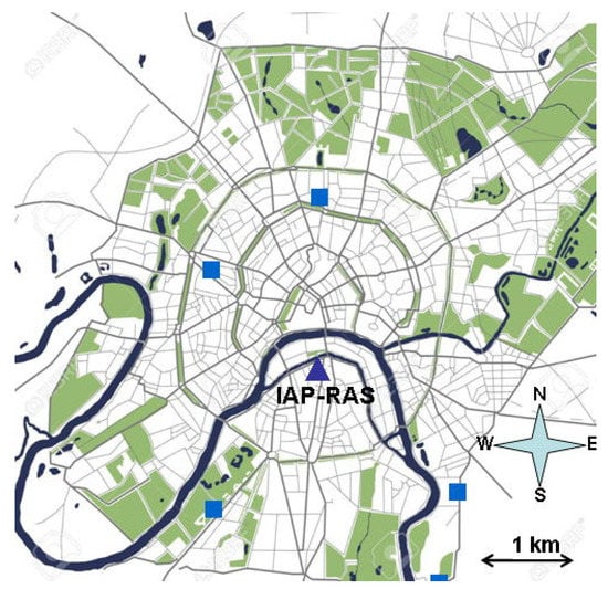
Figure 1.
Spatial locations of IAP-RAS (filled triangle) site and MOSECO urban air quality monitoring sites (filled squares) on a map of the central part of Moscow city (downloaded from Dreamstime.com).
Measurements were made from September 2019 to July 2020 using an automatic computer-aided measurement system developed in IAP [3,23,24]. The main instrument for measurements was a compact-type proton-transfer-reaction mass spectrometer (PTR-MS), provided by Ionicon Analytik GmbH (Austria) in 2008. To control the instrument and to calculate measured concentrations, the native software PTR-MS Control, version 2.7.1.302, was used. The main principles of PTR-MS operation can be found in many papers, for instance, [25]. The working parameters of PTR-MS operation were the following: primary ions were H3O+, E/N = 149.9 Td (1 Td = 10–21 V m2) when Udrift = 600 V, pdrift = 2.0 mbar and Tdrift = 333 K (60 °C) as default factory values. The levels of impurity ions NO+ (m/z 30), O2+ (m/z 32) and cluster ions H3O+(H2O) (m/z 37) did not exceed 0.1–0.2%, 3–4% and 0.3–0.4%, respectively, of the primary ion levels during measurements. Measured components and their corresponding m/z values are given in further text. Guidelines for choosing m/z values were taken from [25,26], taking into account that in some cases the 2-methyl-3-buten-2-ol (MBO) fragmentation could interfere isoprene signal at m/z 69.070 [27,28]. The modern method to divide MBO and isoprene using NO+ mode [29] seems to be not applicable to our earlier type of PTR-MS. In the subsequent discussion we imply data at m/z 69.070 as total sum of isoprene and MBO fragment, taking into account that at the IAP site area isoprene seems to be the dominant specie at this m/z [3,24,30,31]. Monoterpenes were detected as the sum of m/z 137.129 and m/z 81.070 signals as total monoterpenes [24]. Dwell time was set at 0.5 s for all measured m/z channels.
Additionally, carbon monoxide (CO) concentration was measured using the 48 S instrument provided by Thermo Inc. (USA) with a 60 sec response time and a range limit of 0.05–10 ppmv. Ozone (O3) concentration was measured by the 1008-AH instrument provided by Dasibi Inc. (USA) with the same response time and a range limit of 1–1000 ppbv.
All instruments were placed inside special all-weather racks, temperature-controlled at +32 °C and located in open air. Air inlets were downward funnels located 2.5 m above ground, with PTFE tubing with 1/4” OD and 3 m length, individual for each instrument. These tubes were not specially heated. The tube destined for PTR-MS was connected to the 1 m long PTR-MS inlet tube heated at 60 °C. Tubes for CO and O3 analyzers have 5 μm PTFE filters installed, and the PTR-MS tube has no filter to prevent it from destroying VOCs. Problems with particles blocking the capillaries inside the PTR-MS were successfully solved by replacing (or cleaning in some cases) the capillary when it became blocked, approximately one or two times per year. Air flow in these tubes was maintained at 1.0 L/min for PTR-MS and 2.0 L/min for CO and O3 analyzers.
For PTR-MS calibration purposes, permeation tubes were used. These were provided by Mendeleev Research Metrology Institute, Russia (for benzene and toluene), and by VICI Metronics Inc., Poulsbo, WA, USA (for isoprene and alpha-pinene). A detailed description of tubes provided by VICI Metronics Inc. can be found at: https://www.vici.com/calib/perm_dyna.php (accessed on 10 December 2021), in the section “Perm tube”. Tubes provided by Mendeleev Research Metrology Institute (Russia) are the same. To operate with permeation tubes, the gas generator GDP-102, produced by “Analitpribor” (Russia), and the zero air generator Sominix 3057, provided by LNI Swissgas SA (Switzerland), were used. The working parameters of all permeation tubes are presented in Table 1.

Table 1.
Working parameters of permeation tubes.
During calibration, measured concentrations from all permeation tubes were found to differ from theoretically predicted values by no more than 10%, so no additional calibration coefficients were added.
The CO meter was calibrated monthly by gas standards provided by Mendeleev Institute, mentioned above.
Data averaged by 1 min intervals from all instruments were then prepared for further analysis.
2.2. Meteorology
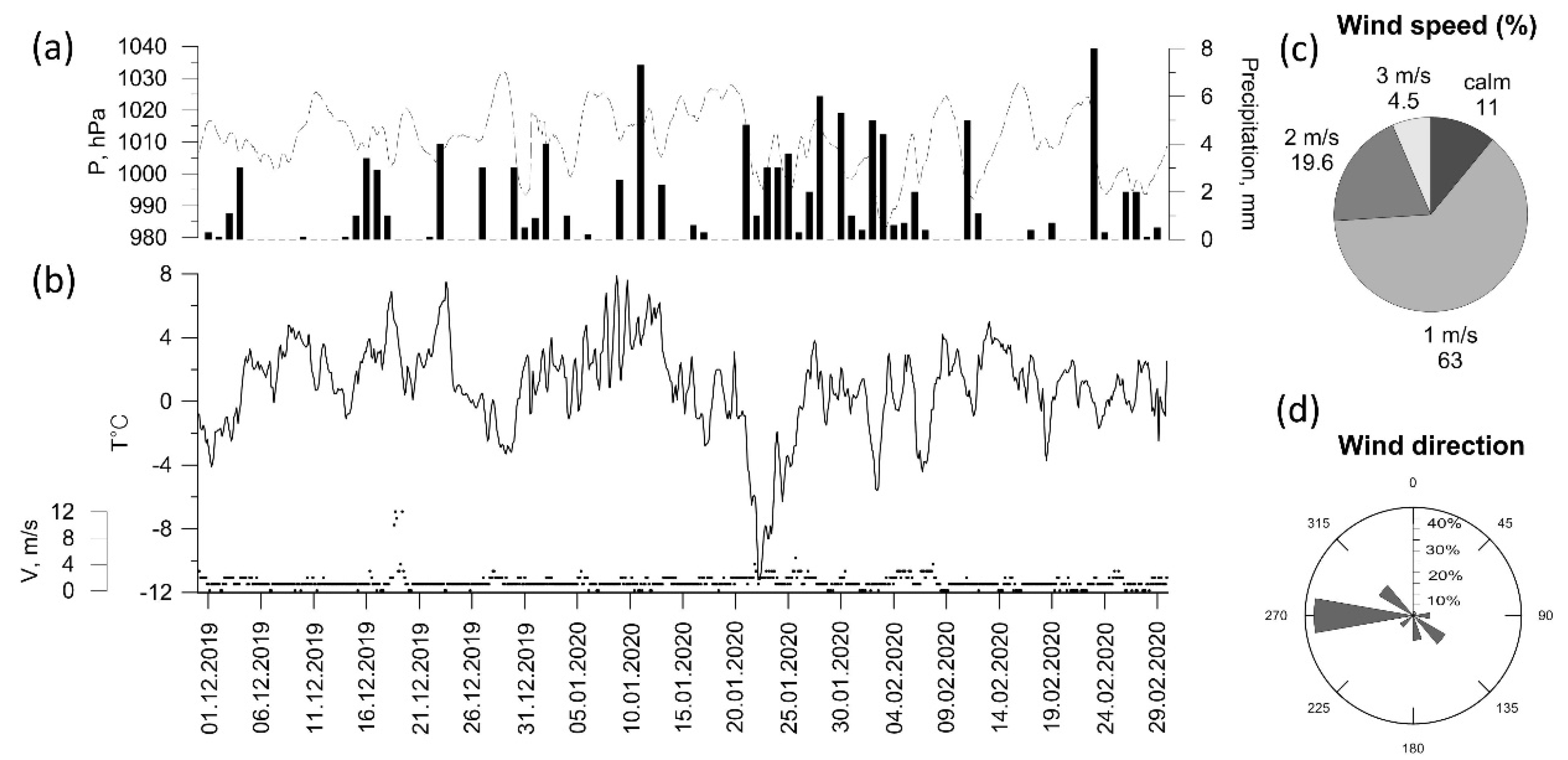
To describe the meteorological conditions around the IAP-RAS site, meteorological data from the Balchug meteorological station (WMO ID 27605), located ~1 km to the north, were employed. In general, autumn 2019 was quite dry (less than mean autumn precipitation), with air temperatures being close to their climatic values (Table 2). Winter 2019–2020 in Moscow was the warmest during the whole period of instrumental observations (from 1961 to 1990) with no stable snow cover (Table 2, Figure 2b). In the center of Moscow, snow cover was observed only for 4 days in December and for 18 and 20 days in January and February, respectively. The seasonal average temperature was about † 1 °C, which is more than 7 °C higher compared to the climatic mean (Figure 2b). Westerly winds prevailed throughout the winter, and average wind speed did not exceed 1 m/s for about two-thirds of the total observation time Figure 2c,d). High-wind conditions with wind speed up to 14 m/s were recorded only on one day in December (19 December).
Table 2.
Average monthly meteorological data for Balchug for the period September 2019–July 2020.

Figure 2.
Meteorological variables (a–d) at Balchug station in winter 2019–2020 (3 h observations).
The end of spring and early summer were rainy, with precipitation ranging from 200 to 300% of the mean monthly values. The summer of 2020 was rainy and warm (Figure 3a,b). Air temperature exceeded 25 °C in 17% of observations. The average wind speed (Figure 3c) did not exceed 1 m/s in 50% of occurrences and was >3 m/s only in 3% of occurrences. West and east wind directions dominated at the IAP-RAS site region (Figure 3d).
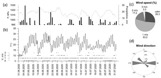
Figure 3.
Meteorological variables (a–d) at Balchug station in summer 2020 (3 h observations).
For the present analyses, all original data on the species mixing ratios were aggregated at 1 h time intervals to suppress the poorly controlled impact of short-time fluctuations within the planetary boundary layer (PBL) turbulence on the final estimates. Close inspection of the data, however, reveals strong episodic fluctuations in the measured species mixing ratios on time scales from tens of minutes to hours, producing partly inconsistent temporal behavior of some VOCs, as judged from visual inspection of the data and the estimated low correlations between species with qualitatively similar emission sources (i.e., benzene and C8 aromatics, whose primary anthropogenic source is strongly associated with vehicle exhausts). Such fluctuations were found to be closely associated mainly with winds blowing from 180–360° directions from a densely built area characterized by complex and poorly constrained pollutant emission sources. We then deleted the 1 h time intervals associated with strong short-term data variability to finally obtain the filtered 1 h dataset of the measured species, which was used in the subsequent analysis.
It is worth noting that the measured levels of CO and VOCs at the IAP-RAS site in a particular hour of day did not exceed their maximum permissible levels in the period of observation (e.g., maximum measured wintertime CO mixing ratio of ~0.4 ppmv vs. the respective maximum allowable 8 h average of 30 ppmv).
Thus, low winds (0–2 m/s) both in summer and in winter can contribute to the accumulation of pollutants near the IAP-RAS site due to local emissions providing a screening effect for more distal urban sources.
3. Results
3.1. Ozone Formation Potential of VOCs
The maximum incremental reactivity method [32] was applied to summer daytime (12:00–18:00 LT) data to estimate the ozone formation potential (OFP) of individual VOCs (see Table 2) at the IAP-RAS site. OFP is calculated using the following formula:
where CVOC is a VOC concentration having the dimension µg/m3, and MIRVOC is the maximum incremental reactivity, a dimensionless quantity defined as grams of O3 produced per gram of the VOC. The method allows for estimating the maximum ozone concentration produced from the chemical destruction of the given VOC based on predefined MIRVOC values.
OFP[µg/m3] = CVOC × MIRVOC
The highest OFP values were obtained for acetaldehyde, ethanol, 1.3-butadiene, isoprene, toluene and C-8 aromatics (Table 3, in bold). This agrees closely with our previous estimates [3] based on the 2011–2013 VOC measurements at the Moscow State University IAP-RAS site located ~10 km SW from the IAP–RAS site in a relatively cleaner environment. In 90% of cases, the OFP of all measured VOCs at the IAP site did not exceed 45 µg/m3. This compares to, although systematically lower than, the corresponding 90th percentile OFP value at the MSU-IAP station (100 µg/m3). The observed lower OFPs of individual species and the total OFP for the 2019–2020 dataset can be explained by lower concentrations of VOCs at the IAP site compared to the respective summertime (2011–2013) values at the MSU-IAP site [3], which is most likely attributed to the COVID-19 situation in Moscow and the accompanying decrease in VOC vehicle exhausts. The other probable reason for lower OFPs in summer 2020 is unfavorable meteorological conditions, with the total number of days with high radiation and air temperatures >25 °C accounting for only 17% in June–August, inhibiting photochemical ozone generation in the urban PBL. The total OFP of acetaldehyde, ethanol, 1.3-butadiene, toluene, isoprene and C-8 aromatics was estimated to be ~26 µg/m3 on average, which amounts to 82% of the total ozone formation potential of all VOCs listed in Table 3. We focus on the above VOCs in the subsequent discussion, as their near-surface abundance is indicative of the strength of primary sources of atmospheric contamination that are most important for the urban ozone photochemistry in Moscow.
Table 3.
Daytime ozone formation potentials (in µg/m3) for VOCs measured at IAP site in summer 2020 (269 valid 1 h observations in total): mean—sample mean; σ—standard deviation; P10, P90—percentiles of the data; methyl vinyl ketone + methacrolein (MVK + MACR) represents isoprene products.
3.2. Annual Variations in CO and VOCs in Moscow
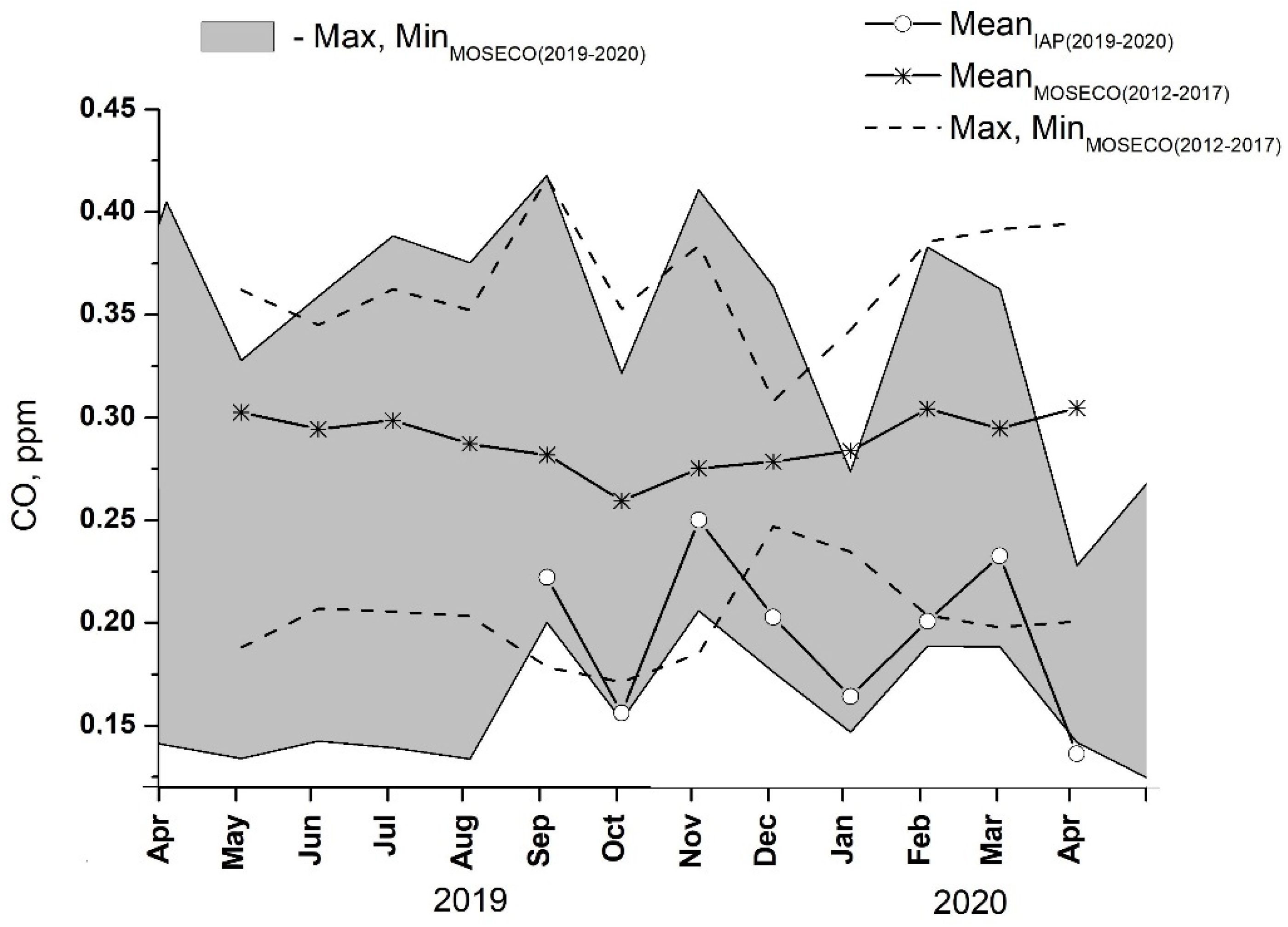
The seasonal cycle of mean carbon monoxide for the reduced period of CO measurements at IAP-RAS from September 2019 to April 2020 is shown in Figure 4. In the figure, a min–max range of the monthly CO values observed for the same period at five nearby urban air quality monitoring sites (Figure 4) belonging to the MOSECO network is also provided. There is a substantial difference in the monthly CO abundances among the MOSECO sites, with individual mixing ratios ranging from <0.15 to 0.4 ppmv. This may indicate the great impact of local environments (i.e., surrounding buildings and associated local circulations) as well as the effects of strong variability in the strength of nearby pollutant sources on surface data. It can be seen that throughout the year, CO mixing ratios at IAP-RAS are close to the lower end of the overall spread of the data (gray area in Figure 4), reflecting an across-city NW–SE increase in pollutant abundance according to the prevailing W to NW winds in the region.

Figure 4.
Annual cycles of monthly mean CO mixing ratios at IAP ̶ RAS (solid, open circles) and 5 urban air quality monitoring sites (MOSECO network, Figure 1) (min–max range, shaded) for the May 2019–April 2020 observation period. For comparison, CO data at MOSECO network: mean (upper solid) and min–max (dashed) of monthly averages for the preceding 5-year period from 2012 to 2017 are provided.
Noting abnormal weather conditions during both winter and summer in the 2019–2020 measuring period at IAP-RAS, the 2019–2020 IAP-RAS and MOSECO CO data were compared against MOSECO measurements at the same sites for the preceding period from 2012 to 2017 (Figure 4), with the latter dataset being assumed to represent some climatic average seasonal tendencies. A general agreement between the 2019–2020 and 2012–2017 MOSECO CO datasets can be seen in terms of the overall data spread among the measurement sites. It could be concluded that amplitudes of interannual variability in pollutant levels in the city (with CO being considered a proxy for the other pollutants) are well within the range of variability among individual sites. This strongly supports the general notion of the dominant role of local emission sources and wind regimes as principal factors that control pollutant abundances in the surface layer over the city.
According to Figure 4, the 2012–2017 average seasonal cycle in CO has a maximum in April and a minimum in October, with an approximate amplitude of 0.05 ppmv, thus demonstrating some resemblance to the well-known annual variation in baseline CO in the Northern Hemisphere extratropics [33], as well as aged air masses from Western Europe [34,35] and continental areas of North Eurasia [36,37]. Using CO mixing ratios of 0.18 and 0.1 ppmv as representatives for the continental mixing layer in midlatitudes in winter and summertime, the local contribution of urban sources to the measured CO levels in the surface air over Moscow can be estimated to be approx. 0.15 ppmv throughout most of the year. The only exception is autumn months, during which a lower input of about 0.13 ppmv is seen, most likely due to the prevailing wind directions and cyclonic weather conditions in the region, which are unfavorable for near-surface accumulation of pollutants from both local and regional pollution sources.
Close inspection of Figure 4 shows much lower CO mixing ratios at the IAP-RAS site compared to the above-discussed 2012–2017 mean seasonal cycle. This can be partly attributed to the above-mentioned across-city gradient in pollutant load as well as to the abnormal weather conditions during the 2019–2020 winter season, which were unfavorable for near-surface accumulation of the emitted pollutants. Consequently, the observed monthly average January 2020 CO mixing ratio of 0.17 ppmv is about 0.12 ppmv lower compared to the respective 2012–2017 mean and compares well with the baseline continental value in winter.
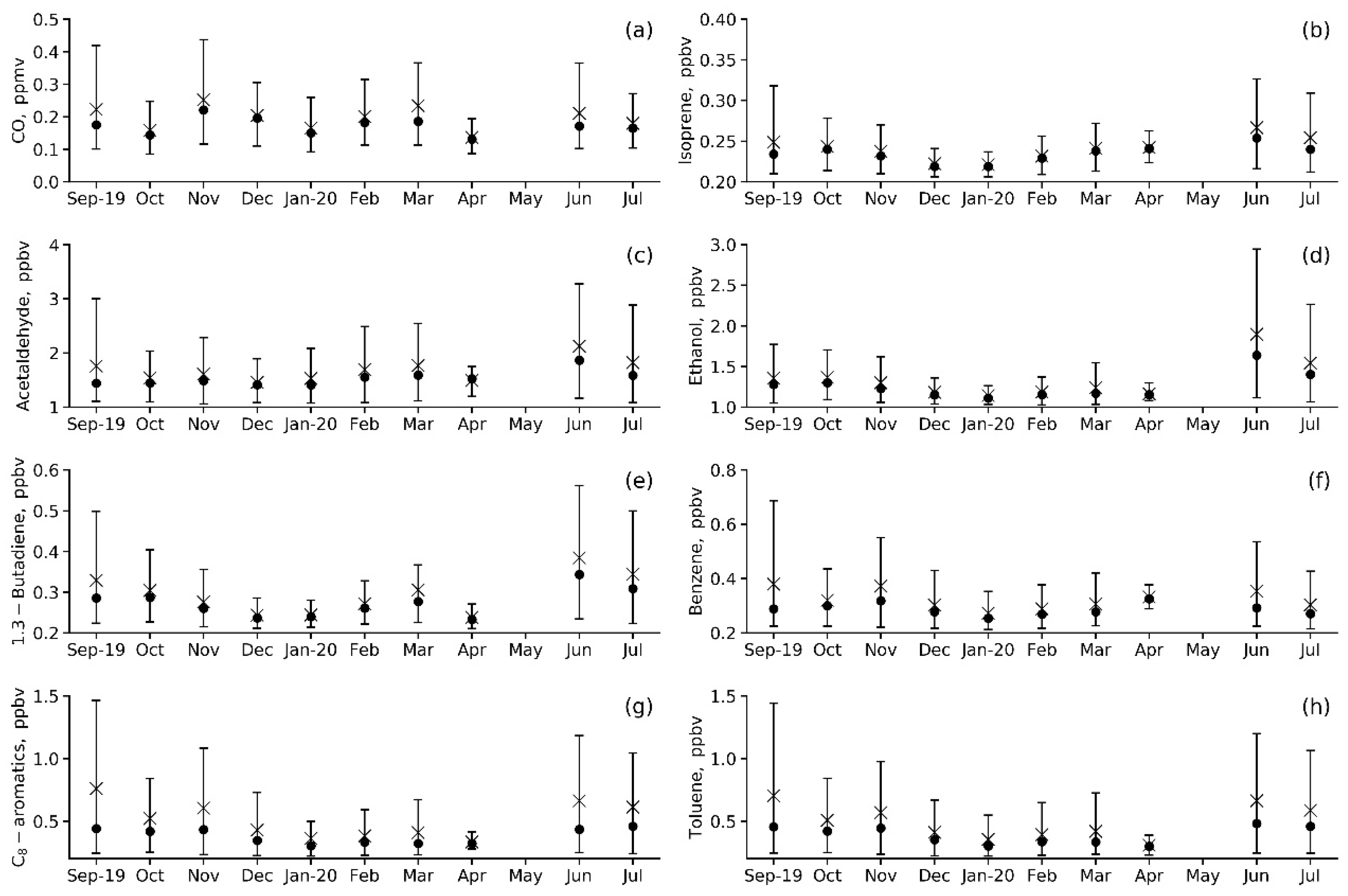
Compared to CO (Figure 5a), much shorter lifetimes are characteristic of other VOCs, so their abundance is essentially controlled by local (urban-scale) emissions. Nevertheless, annual variations in primary anthropogenic VOCs (benzene, toluene, 1.3-butadiene and C-8 aromatics) are similar to those in CO (Figure 5e–h). They are characterized by moderately strong variations in daily mean values, with the maximum variability in daytime values being observed in autumn and summer. Acetaldehyde and ethanol can be both primary and secondary. Therefore, we can see the marked maximum in mean values and wide scattering in the concentrations of these VOCs in summer months, when photochemical oxidation in the troposphere is the most active (Figure 5c,d). Annual variation in isoprene (Figure 5b) is similar to that in other biogenic VOCs, with the observed annual maximum reached in vegetation periods (June, July and September). However, the summertime isoprene levels are generally low, approaching the observed summertime levels of 0.1–0.5 ppbv (0.28 ppbv on average, Table 4) in rural areas of the European part of Russia [30,38] because of the small vegetation area around the IAP site. All VOCs except isoprene and benzene showed the lowest mean concentration in April, which is when vehicle exhausts decreased due to the COVID-19 lockdown.
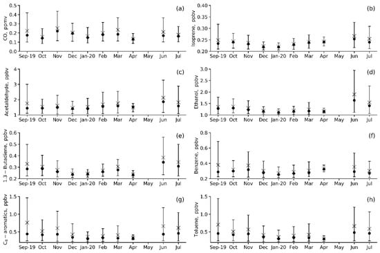
Figure 5.
Annual variations in the measured VOC species mixing ratios (a–h) at IAP-RAS for the May 2019–April 2020 observation period. Mean is an asterisk, median is a circle, and P10–P90 range is a vertical bar.
Table 4.
The 2019–2020 seasonal average species mixing ratios (ppbv) at the IAP-RAS in Moscow.
3.3. Diurnal Variations in CO and VOCs
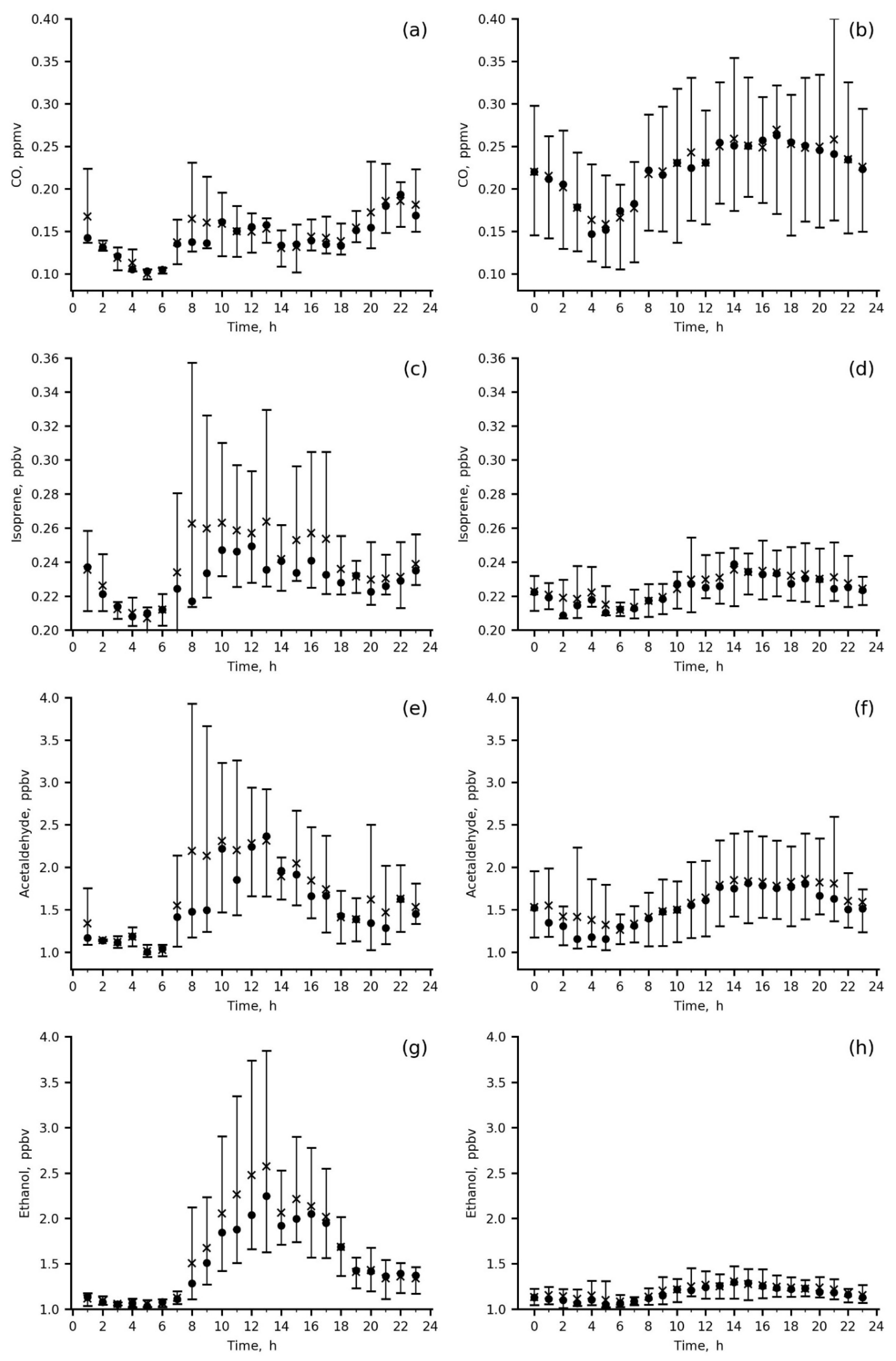
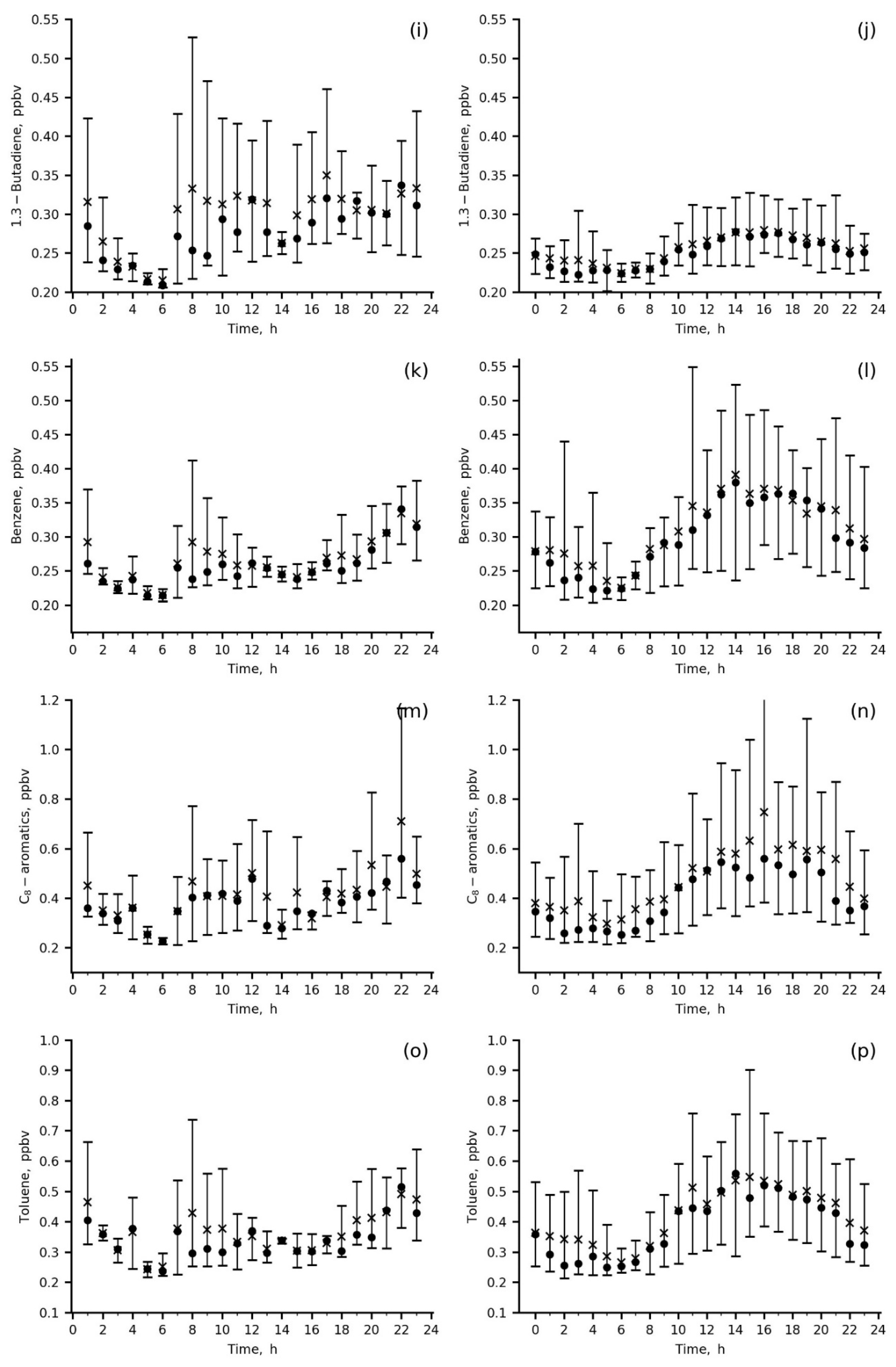
Mean diurnal cycles and total variations for CO and major VOCs species (Table 3) in the winter and summer months of the 2019–2020 observation period are shown in Figure 6.
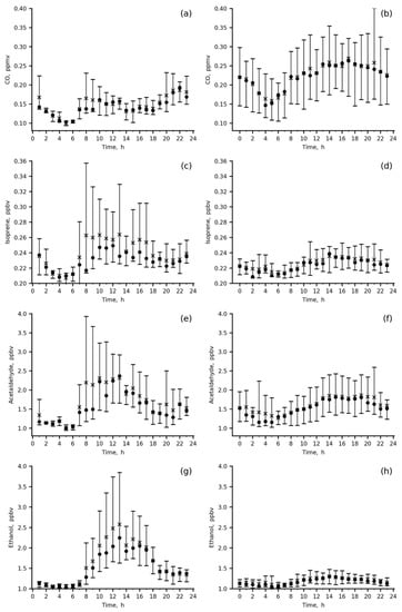

Figure 6.
Diurnal variations in the measured species mixing ratios at IAP site in summer 2020 (a,c,e,g,i,k,m,o) and in winter 2019–2020 (b,d,f,h,j,l,n,p); wind direction was 0–180 deg., mean (asterisk), median (circle), P10–P90 range (vertical bar).
The diurnal variations in CO and primary anthropogenic VOCs, benzene, toluene, C-8 aromatics and 1.3-butadiene, are quite similar, with a smooth increase during the day from 06 a.m. to 22 p.m. local time (LT) in winter and with two peaks, in the morning (06–10 a.m. LT) and in the evening (18–22 p.m. LT) in summer (Figure 6a,b,i–p). In winter, both the mixing ratios of the above VOCs and their variability were higher than those in summer due to their accumulation in the poorly ventilated surface layer (wind speeds = 0–1 m/s) and weak daytime photochemistry, resulting in species abundances being more preconditioned upon a particular weather pattern.
Secondary (acetaldehyde and ethanol) and biogenic (ethanol and isoprene) VOCs (Figure 6c–h) were the highest in summer morning to midday hours (08 a.m.–16 p.m. LT) because biogenic emissions of isoprene and ethanol from either sparse local vegetation or more distant green areas upwind contributed to the measured mixing ratios. The important role of biogenic emissions in the present data is evidenced by the direct comparison between summertime and wintertime isoprene data, showing increases in both mean daytime isoprene levels and their variability for the former. An anthropogenic impact (vehicle exhaust) is clearly seen from the winter increase in acetaldehyde, ethanol and isoprene during the day (18–22 p.m. LT), similar to primary anthropogenic VOCs. For acetaldehyde, the impact of vehicles is also confirmed by the morning peak in summer (up to 4 ppbv).
Wintertime concentrations of secondary and biogenic VOCs clearly reflect an impact of anthropogenic urban emissions (mainly vehicle exhausts) on their levels (Figure 6d,f,h). Below, we quantify this impact and estimate emission ratios of the main ozone precursors measured at the IAP site.
3.4. Determination of VOC Emission Ratios
Typically, the quantitative information of VOC emissions is presented in two basic forms: the emission factor (EF) and the emission ratio (ER) [21,22]. The ER of a VOC is calculated using the two-sided linear regression fit (LRF) method as ER = ΔY/ΔX, where X is an inert tracer, representing the predominant emission from a single type of source and does not evolve significantly due to photochemistry or other processes in a short time scale. It is very difficult to ignore the impact of mixing from multiple sources and photochemical processes due to the short lifetimes of VOCs in ambient air in urban environments. Therefore, the estimated ERs of ΔVOC/ΔX include uncertainties due to post-emission processes.
We used mixing ratios of both benzene and CO as tracers for anthropogenic emissions to calculate ERs. The 1 h measurements of VOCs on days with wind direction = 0–180 deg. were selected for the analysis.
To take into account only the effect of local pollution, the T/B ratio filter was used [39,40,41,42]. The calculated T/B ratio for summer (Figure 7b,d) and winter (Figure 7a,c) data was mainly in the range of 0–3. Data with T/B ratios of 1–2 were chosen for further analysis because they reflect local emissions as the predominant source of VOC pollution at the IAP site.
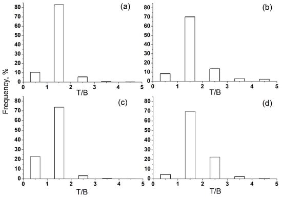
Figure 7.
T/B ratio for summer and winter data in Moscow in 2020. (a) winter, day; (b) summer, day; (c) winter, night; (d) summer, night.
To neglect the change in VOC composition due to the absence of OH oxidation and the influence of their light-dependent biogenic emissions, the 1 h nighttime data (22–06 LT) filtered on T/B = 0–2 and wind direction = 0–180 deg. were used to calculate the ERs.
There is a good correlation between CO and benzene at nighttime in winter (Figure 8). This points to primary vehicle exhaust being a dominant source of local CO emissions at the IAP site.
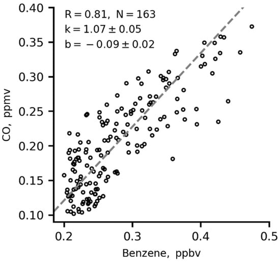
Figure 8.
Two-sided (orthogonal) regression fits for 1 h averages of CO versus benzene at nighttime in winter. K is the slope in the orthogonal regression fit.
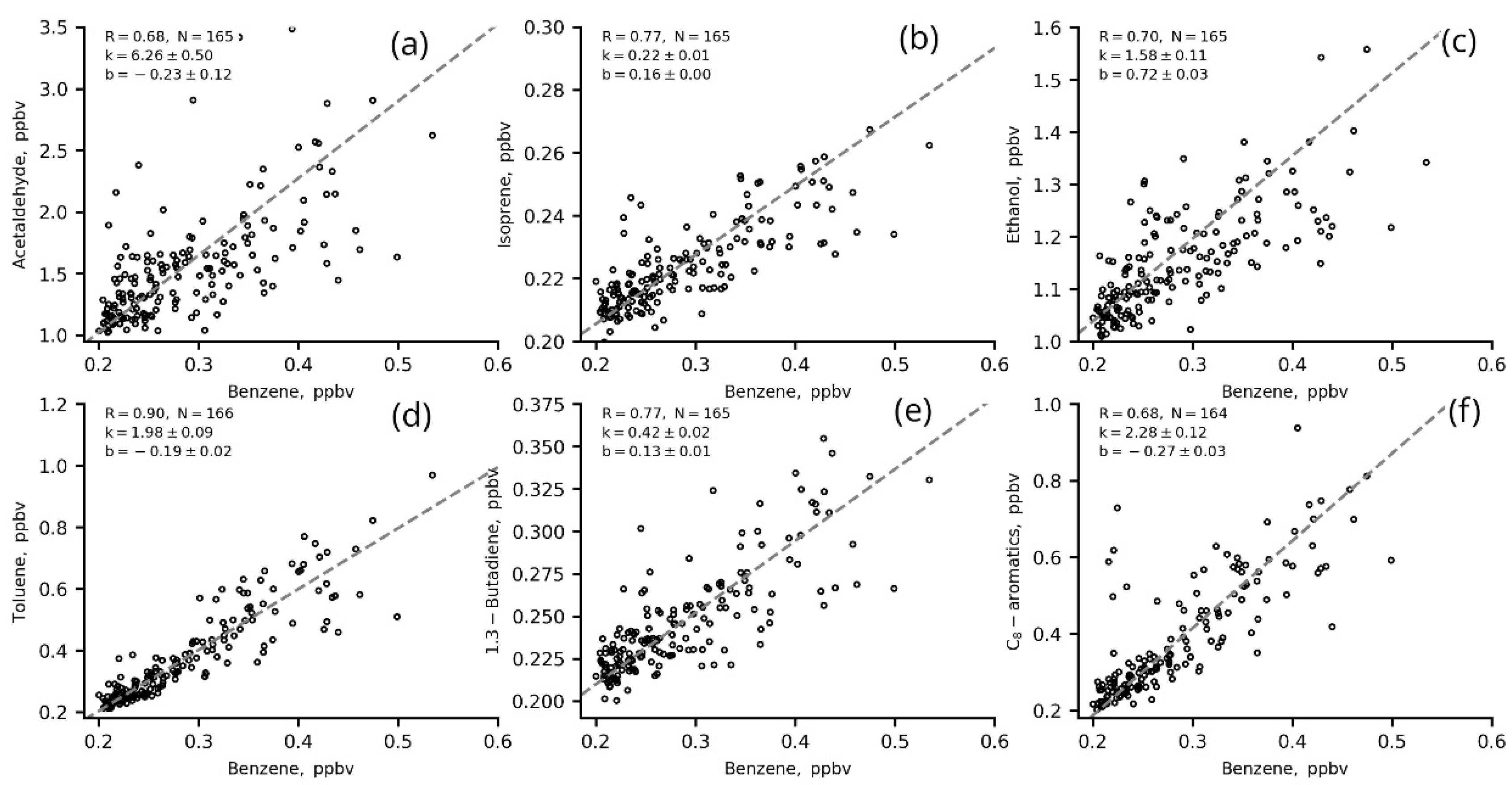
The ERs (slopes, k, in two-sided linear regression fits for VOCs versus benzene and CO) for the most significant VOCs in ozone production from IAP site measurements in winter (01 January–31 February) 2020 are presented in Figure 9 and Figure 10 and in Table 5.

Figure 9.
Two-sided linear regression fits for VOCs (a–f) to benzene (1 h data) in winter 2020 (22–06 LT, T/B = 1–2.

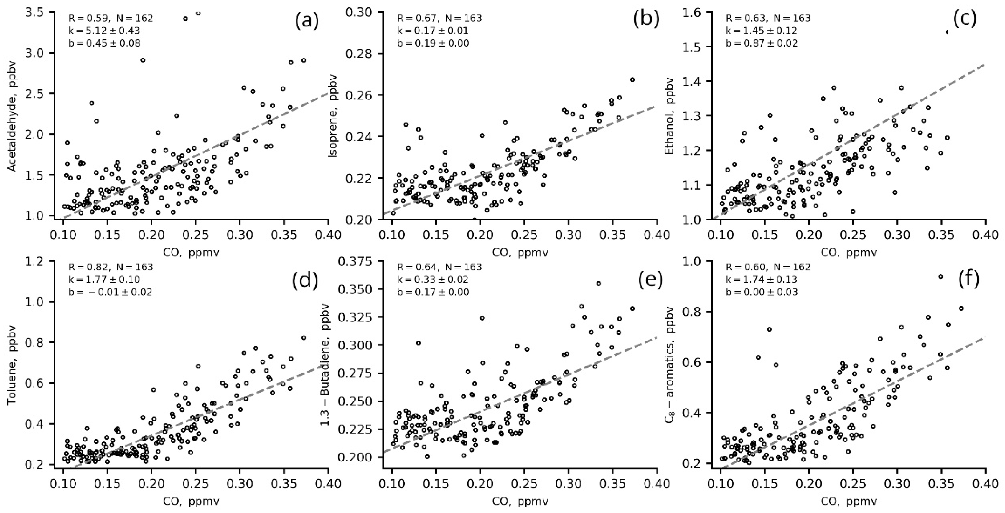
Figure 10.
Two-sided linear regression fits for VOCs (a–f) to CO (1 h data) in winter 2020 (22–06 LT, T/B = 1–2).
Table 5.
Winter nighttime ERs of VOCs estimated versus benzene (ppbv/ppbv benzene) and CO (ppbv/ppmv CO) from winter IAP site data (2019–2020). R—correlation coefficient.
Most of the VOCs correlated well with benzene (R > 0.6), including those that are usually associated with biogenic emissions and/or secondary VOCs such as acetaldehyde, ethanol and isoprene (Figure 9 a–c). This indicates that these VOCs share a common source with benzene (e.g., vehicle exhausts) in regard to evaporation, for example. The correlation of these VOCs with CO is worse. This may be due to the long lifetime of CO in the atmosphere and the complexity of its urban sources. The winter nighttime slopes (ERs) for VOCs versus benzene are slightly higher than those for VOCs versus CO (Figure 10, Table 5), which suggests that VOC concentrations have a better response to benzene changes than to CO changes.
The ERs of VOCs estimated in the present study are close to the values estimated for other megacities [20,21,31,43]. The ER of acetaldehyde (5.12 ppbv/ppmv CO and 6.26 ppbv/ppbv benzene) is similar to the ERs obtained for Los Angeles (5.42 pptv/ppbv CO and 5.42 ppbv/ppbv CO) by [20,43] and for London (4.14 pptv/ppbv CO) estimated in [43]. The ER of isoprene (0.17 ppbv/ppmv CO and 0.22 ppbv/ppbv benzene) is similar to the estimates for Los Angeles and Mexico (0.30 pptv/ppbv CO and 0.08 pptv/ppbv CO, respectively [20,43]) but less than for Saõ Paulo (1.17 pptv/ppbv CO [43]) and London (1.13 [31,43]). The ER of toluene (1.77 ppbv/ppmv CO and 1.98 ppbv/ppmv benzene) is similar to London estimates (1.94 pptv/ppbv CO [43]), and the ER of C-8 aromatics (1.74 ppbv/ppmv CO and 2.28 ppbv/ppbv benzene) is comparable to the estimations for Saõ Paulo (2.15 pptv/ppbv CO [43]) and Los Angeles (2.45 pptv/ppbv CO [20]).
The calculated ERs show better estimations of the anthropogenic impact on VOC levels with the use of benzene as a tracer. Thus, we used ERsbenzene for further estimations of VOC anthropogenic fractions at the IAP site.
3.5. Source Identification of VOC Emissions
To quantify the relative contributions of primary emissions and secondary formation of VOCs (as well as biogenic emissions), anthropogenic fractions of VOCs (AFs) were estimated [20,21,44] from their nighttime (22–06 local time) winter ERsbenzene values (see Table 5) using the relation:
where ERΔVOC/Δbenzene is the estimated nighttime emission ratio for winter; CONCbenzene is the measured benzene mixing ratio in ppbv.
AF = ERΔVOC/Δbenzene × CONCbenzene
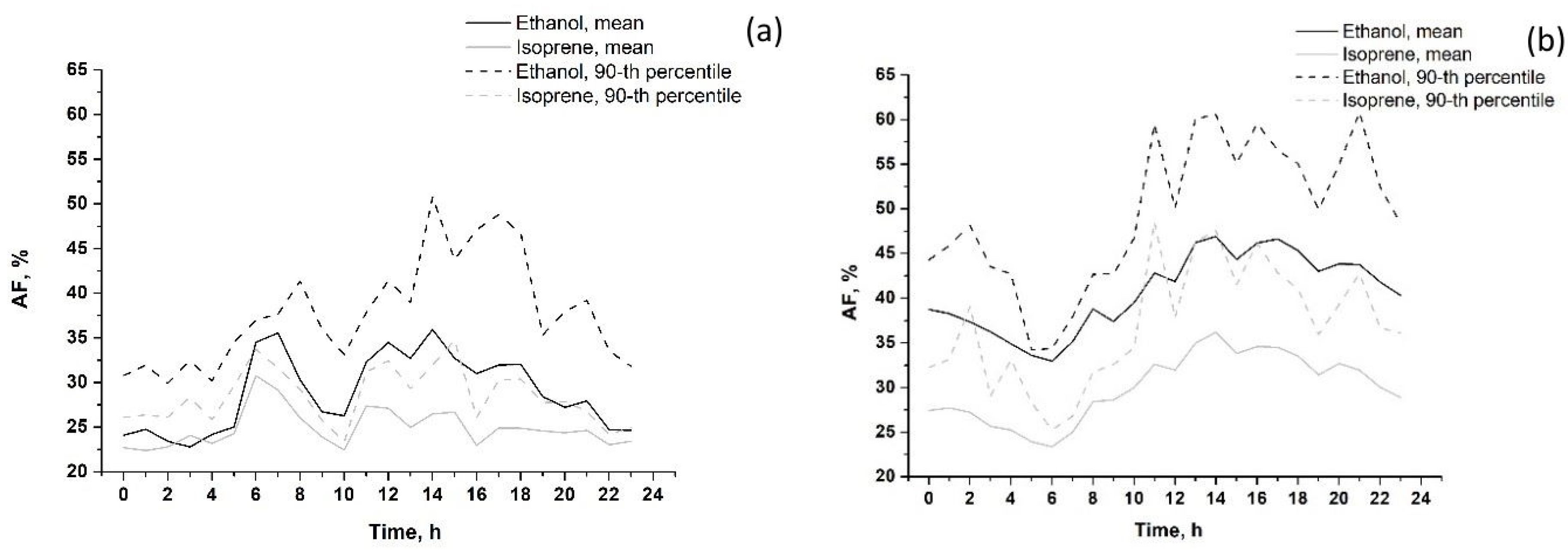
The calculated diurnal variations in AFs (in %) in summer and in winter 2020 are shown in Figure 11.
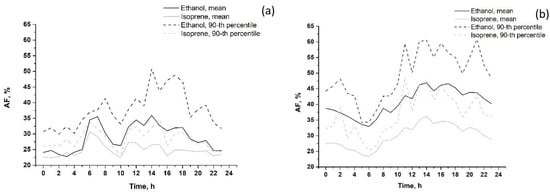
Figure 11.
Diurnal variations in anthropogenic fractions (AF value, %) of VOCs (mean and 90th percentile) in summer 2020 (a) and in winter 2019–2020 (b). VOCs that are not shown on the graphs (acetaldehyde, toluene, 1.3-butadiene and C8 aromatics) have a 100% vehicle source.
As expected, acetaldehyde, toluene, 1.3-butadiene and C8 aromatics were entirely anthropogenic (urban vehicle exhausts) throughout the day, both in summer and in winter. In summer, the mean AF of isoprene did not exceed 35%, and the mean AF of ethanol did not exceed 50% throughout the day. AFs of both VOCs increased slightly from 6 to 8 p.m. and from 10 a.m. to 15 p.m. due to more active traffic during these hours. In winter, the mean anthropogenic fractions of isoprene and ethanol increased from 8 a.m. to 14 p.m. up to 35% and 60%, respectively, which is typical for the other anthropogenic VOCs described above. The remaining parts of isoprene and ethanol emissions are due to biogenic and photochemical impacts (up to 65–70% for isoprene and 40–50% for ethanol). In summer, the corresponding EFs of isoprene and ethanol were 5–10% and 10–20% lower compared to those in winter. The above feature can be explained by the greater impact of biogenic emissions and photochemistry on near-surface VOC abundance in summer. However, the estimated low AFs of ethanol and isoprene in winter are in question since the contribution of non-anthropogenic sources (biogenic and photochemical) is expected to be relatively small in winter months.
4. Conclusions
The measurements of CO and 15 volatile organic compounds (VOCs) at the IAP-RAS site located in the center of Moscow city were analyzed. Acetaldehyde, ethanol, 1.3-butadiene, isoprene, toluene and C-8 aromatics were found to be the main ozone precursors in the city, providing up to 82% of the total ozone formation potential of the VOCs measured. The concentrations of anthropogenic VOCs (acetaldehyde, benzene, 1.3-butadiene, toluene and C-8 aromatics) did not exceed their maximum permissible levels, reaching their annual maxima in summer and in the autumn morning and evening hours. The amplitudes of interannual variability in pollutant levels at the Moscow sites are well within the range of variability among individual cities. This strongly supports the general notion of the dominant role of local emission sources and wind regimes as principal factors controlling pollutant abundances in the surface layer over the city.
Diurnal variations of CO and primary anthropogenic VOCs (benzene, toluene, C-8 aromatics and 1.3-butadiene) were quite similar, showing maxima in the morning (06–10 a.m. LT) and evening (18–22 p.m. LT) hours in summer. Both mixing ratios and short-term variability in CO and primary anthropogenic VOCs (benzene, toluene, C-8 aromatics and 1.3-butadiene) were highest in winter due to their accumulation in the poorly ventilated surface layer (wind speeds = 0–1 m/s) and weak daytime photochemistry, resulting in species abundances being more preconditioned upon a particular weather pattern.
Secondary (acetaldehyde and ethanol) and biogenic (ethanol and isoprene) VOCs were highest in summer morning to midday hours (08 a.m.–16 p.m. LT), presumably because of the biogenic emissions of isoprene and ethanol, as well as higher rates of oxidation of primary VOC species leading to the seasonal increase in acetaldehyde and ethanol mixing ratios. The important role of biogenic emissions in the present data is evidenced by the direct comparison between summertime and wintertime isoprene mixing ratios, showing increases in both mean daytime isoprene levels and their variability in summer. However, the measured wintertime abundances of the secondary and biogenic VOCs clearly reflect an impact of anthropogenic urban emissions (mainly vehicle exhausts) on their levels throughout the year.
Anthropogenic fractions of acetaldehyde, toluene, 1.3-butadiene and C8 aromatics were found to be close to unity during the whole day throughout a year, with the urban vehicle exhausts being the primary origin of these species. Anthropogenic fractions of isoprene and ethanol did not exceed 0.3 and 0.5 in summer, pointing to proportionally higher contributions of their biogenic sources. However, the estimated low anthropogenic factors of the above species in winter are in question since the contribution of the biogenic signal is expected to be weak in winter months.
Author Contributions
All author s contributed to the original draft preparation of the manuscript; I.B. and V.B. conceived and designed the experiments; E.B., A.V. and N.P. contributed to the data analysis; A.S. and K.M. provided project administration and revised the whole manuscript. All authors have read and agreed to the published version of the manuscript.
Funding
This work was funded by the Russian Science Foundation under grant №. 21-17-00021 (data analysis) and by grant No. 075-15-2021-934 in the form of a subsidy from the Ministry of Science and Higher Education of Russia (development of ozone formation scheme).
Institutional Review Board Statement
Not applicable.
Informed Consent Statement
Not applicable.
Data Availability Statement
Not applicable.
Acknowledgments
The authors acknowledge the colleagues from MOSECO for providing CO data for comparison.
Conflicts of Interest
The authors declare no conflict of interest.
References
- Schnell, R.C.; Oltmans, S.J.; Neely, R.R.; Endres, M.S.; Molenar, J.V.; White, A.B. Rapid photochemical production of ozone at high concentrations in a rural site during winter. Nat. Geosci. 2009, 2, 120–122. [Google Scholar] [CrossRef]
- Agyei, T.; Juráň, S.; Edwards-Jonášová, M.; Fischer, M.; Švik, M.; Komínková, K.; Ofori-Amanfo, K.K.; Marek, M.V.; Grace, J.; Urban, O. The Influence of Ozone on Net Ecosystem Production of a Ryegrass–Clover Mixture under Field Conditions. Atmosphere 2021, 12, 1629. [Google Scholar] [CrossRef]
- Berezina, E.; Moiseenko, K.; Skorokhod, A.; Pankratova, N.V.; Belikov, I.; Belousov, V.; Elansky, N.F. Impact of VOCs and NOx on Ozone Formation in Moscow. Atmosphere 2020, 11, 1262. [Google Scholar] [CrossRef]
- Millet, D.B.; Guenther, A.; Siegel, D.A.; Nelson, N.B.; Singh, H.B.; de Gouw, J.A.; Warneke, C.; Williams, J.; Eerdekens, G.; Sinha, V.; et al. Global atmospheric budget of acetaldehyde: 3-D model analysis and constraints from in-situ and satellite observations. Atmos. Chem. Phys. 2010, 10, 3405–3425. [Google Scholar] [CrossRef] [Green Version]
- Kim, S.-W.; McKeen, S.A.; Frost, G.J.; Lee, S.-H.; Trainer, M.; Richter, A.; Angevine, W.M.; Atlas, E.; Bianco, L.; Boersma, K.F.; et al. Evaluations of NOx and highly reactive VOC emission inventories in Texas and their implications for ozone plume simulations during the Texas Air Quality Study 2006. Atmos. Chem. Phys. 2011, 11, 11361–11386. [Google Scholar] [CrossRef] [Green Version]
- Coll, I.; Rousseau, C.; Barletta, B.; Meinardi, S.; Blake, D.R. Evaluation of an urban NMHC emission inventory by measure-ments and impact on CTM results. Atmos. Environ. 2010, 44, 3843–3855. [Google Scholar] [CrossRef] [Green Version]
- Baker, A.K.; Beyersdorf, A.J.; Doezema, L.A.; Katzenstein, A.; Meinardi, S.; Simpson, I.J.; Blake, D.R.; Rowland, F.S. Measurements of nonmethane hydrocarbons in 28 United States cities. Atmos. Environ. 2008, 42, 170–182. [Google Scholar] [CrossRef] [Green Version]
- Parrish, D.D.; Kuster, W.C.; Shao, M.; Kondo, Y.; Goldan, P.D.; de Gouw, J.A.; Koike, M.; Shirai, T. Comparison of air pollutant emissions among mega-cities. Atmos. Environ. 2009, 43, 6435–6441. [Google Scholar] [CrossRef]
- Velasco, E.; Lamb, B.; Pressley, S.; Allwine, E.; Westberg, H.; Jobson, B.T.; Alexander, M.; Prazeller, P.; Molina, L.; Molina, M. Flux measurements of volatile organic compounds from an urban landscape. Geophys. Res. Lett. 2005, 32, L20802. [Google Scholar] [CrossRef]
- Acton, W.J.F.; Huang, Z.; Davison, B.; Drysdale, W.S.; Fu, P.; Holloway, M.; Langford, B.; Lee, J.; Liu, Y.; Metzger, S.; et al. Surface–atmosphere fluxes of volatile organic compounds in Beijing. Atmos. Chem. Phys. 2020, 20, 15101–15125. [Google Scholar] [CrossRef]
- Vaughan, A.R.; Lee, J.D.; Shaw, M.D.; Misztal, P.K.; Metzger, S.; Vieno, M.; Davison, B.; Karl, T.G.; Carpenter, L.J.; Lewis, A.C.; et al. VOC emission rates over London and South East England obtained by airborne eddy covariance. Faraday Discuss. 2017, 200, 599–620. [Google Scholar] [CrossRef] [PubMed] [Green Version]
- Karl, T.; Misztal, P.K.; Jonsson, H.H.; Shertz, S.; Goldstein, A.H.; Guenther, A.B. Airborne Flux Measurements of BVOCs above Californian Oak Forests: Experimental Investigation of Surface and Entrainment Fluxes, OH Densities, and Damkцhler Numbers. J. Atmos. Sci. 2013, 70, 3277–3287. [Google Scholar] [CrossRef] [Green Version]
- Park, C.; Schade, G.W.; Boedeker, I. Flux measurements of volatile organic compounds by the relaxed eddy accumulation methodcombined with a GC-FID system in urban Houston, Texas. Atmos. Environ. 2010, 44, 2605–2614. [Google Scholar] [CrossRef]
- Martin, R.V.; Jacob, D.J.; Chance, K.; Kurosu, T.P.; Palmer, P.I.; Evans, M.J. Global inventory of nitrogen oxides emissions constrained by spacebased observations of NO2 columns. J. Geophys. Res. 2003, 108, 4537. [Google Scholar] [CrossRef] [Green Version]
- Lanz, V.A.; Hueglin, C.; Buchmann, B.; Hill, M.; Locher, R.; Staehelin, J.; Reimann, S. Receptor modeling of C2–C7 hydro-carbon sources at an urban background site in Zurich, Switzerland: Changes between 1993–1994 and 2005–2006. Atmos. Chem. Phys. 2008, 8, 2313–2332. [Google Scholar] [CrossRef] [Green Version]
- Gaimoz, C.; Sauvage, S.; Gros, V.; Herrmann, F.; Williams, J.; Locoge, N.; Perrussel, O.; Bonsang, B.; d’Argouges, O.; Sarda-Estиve, R.; et al. Volatile organic compounds sources in Paris in spring 2007. Part II: Source apportionment using positive matrix factorization. Environ. Chem. 2011, 8, 91–103. [Google Scholar] [CrossRef]
- Morino, Y.; Ohara, T.; Yokouchi, Y.; Ooki, A. Comprehensive source apportionment of volatile organic compounds using observational data, two receptor models, and an emission inventory in Tokyo metropolitan area. J. Geophys. Res. 2011, 116, D02311. [Google Scholar] [CrossRef] [Green Version]
- Warneke, C.; McKeen, S.A.; de Gouw, J.A.; Goldan, P.D.; Kuster, W.C.; Holloway, J.S.; Williams, E.J.; Lerner, B.M.; Parrish, D.D.; Trainer, M.; et al. Determination of urban volatile organic compound emission ratios and comparison with an emissions database. J. Geophys. Res. 2007, 112, D10S47. [Google Scholar] [CrossRef]
- McKeen, S.; Grell, G.; Peckham, S.; Wilczak, J.; Djalalova, I.; Hsie, E.-Y.; Frost, G.; Peischl, J.; Schwarz, J.; Spackman, R.; et al. An evaluation of real-time air quality forecasts and their urban emissions over eastern Texas during the summer of 2006 Second Texas Air Quality Study field study. J. Geophys. Res. 2009, 114, D00F11. [Google Scholar] [CrossRef] [Green Version]
- Borbon, A.; Gilman, J.B.; Kuster, W.C.; Grand, N.; Chevaillier, S.; Colomb, A.; Dolgorouky, C.; Gros, V.; Lopez, M.; Sarda-Esteve, R.; et al. Emission ratios of anthropogenic volatile organic compounds in northern mid-latitude megacities: Observations versus emission inventories in Los Angeles and Paris. J. Geophys. Res. Atmos. 2013, 118, 2041–2057. [Google Scholar] [CrossRef]
- Sahu, L.K.; Yadav, R.; Pal, D. Source identification of VOCs at an urban site of western India: Effect of marathon events and anthropogenic emissions. J. Geophys. Res. Atmos. 2016, 121, 2416–2433. [Google Scholar] [CrossRef] [Green Version]
- Andreae, M.O.; Merlet, P. Emission of trace gases and aerosols from biomass burning. Glob. Biogeochem. Cycles 2001, 15, 955–966. [Google Scholar] [CrossRef] [Green Version]
- Elansky, N.F.; Belikov, I.B.; Berezina, E.V. Atmospheric Composition over Northern Eurasia: The TROICA Experiments; Agrospas: Moscow, Russia, 2009; pp. 73–90. [Google Scholar]
- Berezina, E.; Moiseenko, K.; Skorokhod, A.; Elansky, N.; Belikov, I.; Pankratova, N. Isoprene and monoterpenes over Russia and their impacts in tropospheric ozone formation. Geogr. Environ. Sustain. 2019, 12, 63–74. [Google Scholar] [CrossRef]
- de Gouw, J.; Warneke, C. Measurements of volatile organic compounds in the Earth’s atmosphere using proton-transferreaction mass spectrometry. Mass Spectrom. Rev. 2007, 26, 223–257. [Google Scholar] [CrossRef] [PubMed]
- Taipale, R.; Ruuskanen, T.M.; Rinne, J.; Kajos, M.K.; Hakola, H.; Pohja, T.; Kulmala, M. Technical Note: Quantitative long-term measurements of VOC concentrations by PTR-MS—Measurement, calibration, and volume mixing ratio calculation methods. Atmos. Chem. Phys. 2008, 8, 6681–6698. [Google Scholar] [CrossRef] [Green Version]
- Karl, T.G.; Spirig, C.; Rinne, J.; Stroud, C.; Prevost, P.; Greenberg, J.; Fall, R.; Guenther, A. Virtual disjunct eddy covariance measurements of organic compound fluxes from a subalpine forest using proton transfer reaction mass spectrometry. Atmos. Chem. Phys. 2002, 2, 279–291. [Google Scholar] [CrossRef] [Green Version]
- Vlasenko, A.; Slowik, J.G.; Bottenheim, J.W.; Brickell, P.C.; Chang, R.W.; Macdonald, A.M.; Shantz, N.C.; Sjostedt, S.J.; Wiebe, H.A.; Leaitch, W.R.; et al. Measurements of VOCs by proton transfer reaction mass spectrometry at a rural Ontario site: Sources and correlation to aerosol composition. J. Geophys. Res. 2009, 114, D21305. [Google Scholar] [CrossRef] [Green Version]
- Karl, T.; Hansel, A.; Cappellin, L.; Kaser, L.; Herdlinger-Blatt, I.; Jud, W. Selective measurements of isoprene and 2-methyl-3-buten-2-ol based on NO+ ionization mass spectrometry. Atmos. Chem. Phys. 2012, 12, 11877–11884. [Google Scholar] [CrossRef] [Green Version]
- Jordan, C.; Fitz, E.; Hagan, T.; Sive, B.; Frinak, E.; Haase, K.; Cottrell, L.; Buckley, S.; Talbot, R. Long-term study of VOCs measured with PTR-MS at a rural site in New Hampshire with urban influences. Atmos. Chem. Phys. 2009, 9, 4677–4697. [Google Scholar] [CrossRef] [Green Version]
- Valach, A.C.; Langford, B.; Nemitz, E.; MacKenzie, A.R.; Hewitt, C.N. Concentrations of selected volatile organic compounds at kerbside and background sites in central London. Atmos. Environ. 2014, 95, 456–467. [Google Scholar] [CrossRef] [Green Version]
- Carter, W.P.L. Development of the SAPRC-07 Chemical Mechanism and Updated Ozone Reactivity Scales; Final Report to the California Air Resources Board Contract No. 03-318; California Air Resources Board, Research Division: Sacramento, CA, USA, 2010. [Google Scholar]
- Holloway, T.; Levy, H.; Kasibhatla, P. Global distribution of carbon monoxide. J. Geophys. Res. 2000, 105, 12123–12147. [Google Scholar] [CrossRef]
- Derwent, R.G.; Simmonds, P.G.; Seuring, S.; Dimmer, C. Observation and interpretation of the seasonal cycles in the surface concentrations of ozone and carbon monoxide at mace head, Ireland from 1990 to 1994. Atmos. Environ. 1998, 32, 145–157. [Google Scholar] [CrossRef]
- Derwent, R.G.; Parrish, D.D.; Simmonds, P.G.; O’Doherty, S.J.; Spain, T.G. Seasonal cycles in baseline mixing ratios of a large number of trace gases at the Mace Head, Ireland atmospheric research station. Atmos. Environ. 2020, 233, 117531. [Google Scholar] [CrossRef]
- Pochanart, P.; Akimoto, H.; Kajii, Y.; Potemkin, V.M.; Khodzher, T.V. Regional background ozone and carbon monoxide varia-tions in remote Siberia/East Asia. J. Geophys. Res. 2003, 108, 4028. [Google Scholar] [CrossRef]
- Vasileva, A.V.; Moiseenko, K.B.; Mayer, J.-C.; Jürgens, N.; Panov, A.; Heimann, M.; Andreae, M.O. Assessment of the re-gional atmospheric impact of wildfire emissions based on CO observations at the ZOTTO tall tower station in central Siberia. J. Geophys. Res. 2011, 116, D07301. [Google Scholar] [CrossRef]
- Skorokhod, A.I.; Berezina, E.V.; Moiseenko, K.B.; Elansky, N.F.; Belikov, I.B. Benzene and toluene in the surface air of north-ern Eurasia from TROICA-12 campaign along the Trans-Siberian Railway. Atmos. Chem. Phys. 2017, 17, 5501–5514. [Google Scholar] [CrossRef] [Green Version]
- Tiwari, V.; Hanai, Y.; Masunaga, S. Ambient levels of volatile organic compounds in the vicinity of petrochemical industrial area of Yokohama, Japan. Air Qual. Atmos. Health 2010, 3, 65–75. [Google Scholar] [CrossRef] [Green Version]
- Shaw, M.D.; Lee, J.D.; Davison, B.; Vaughan, A.; Purvis, R.M.; Harvey, A.; Lewis, A.C.; Hewitt, C.N. Airborne determination of the temporospatial distribution of benzene, toluene, nitrogen oxides and ozone in the boundary layer across Greater London, UK. Atmos. Chem. Phys. 2015, 15, 5083–5097. [Google Scholar] [CrossRef] [Green Version]
- Carballo-Pat, C.G.; Cerуn-Bretуn, J.G.; Cerуn-Bretуn, R.M.; Ramнrez-Lara, E.; Aguilar-Ucбn, C.A.; Montalvo-Romero, C.; Guevara-Carriу, E.; Cуrdova-Quiroz, A.V.; Gamboa-Fernбndez, J.M.; Uc-Chi, M.P. Latest trends in Energy. Environment and Development. In Proceedings of the 7-th International Conference on Environmental and Geological Sciences and Engineering (EG’14), Salerno, Italy, 3–5 June 2014; pp. 132–140. [Google Scholar]
- Warneke, C.; van der Veen, C.; Luxembourg, S.; de Gouw, J.A.; Kok, A. Measurements of benzene and toluene in ambient air using proton-transfer-reaction mass spectrometry: Calibration humidity dependence and field intercomparison. Int. J. Mass Spectrom. 2001, 207, 167–182. [Google Scholar] [CrossRef]
- Brito, J.; Wurm, F.; Yáñez-Serrano, A.M.; de Assunção, J.V.; Godoy, J.M.; Artaxo, P. Vehicular emission ratios of VOCs in a megacity impacted by extensive ethanol use: Results of ambient measurements in São Paulo, Brazil. Environ. Sci. Technol. 2015, 49, 11381–11387. [Google Scholar] [CrossRef]
- Reimann, S.; Calanca, P.; Hofer, P. The anthropogenic contribution to isoprene concentrations in a rural atmosphere. Atmos. Environ. 2000, 34, 109–115. [Google Scholar] [CrossRef]


Publisher’s Note: MDPI stays neutral with regard to jurisdictional claims in published maps and institutional affiliations. |
© 2022 by the authors. Licensee MDPI, Basel, Switzerland. This article is an open access article distributed under the terms and conditions of the Creative Commons Attribution (CC BY) license (https://creativecommons.org/licenses/by/4.0/).