Abstract
Machine learning has experienced great success in many applications. Precipitation is a hard meteorological variable to predict, but it has a strong impact on society. Here, a machine-learning technique—a formulation of gradient-boosted trees—is applied to climate seasonal precipitation prediction over South America. The Optuna framework, based on Bayesian optimization, was employed to determine the optimal hyperparameters for the gradient-boosting scheme. A comparison between seasonal precipitation forecasting among the numerical atmospheric models used by the National Institute for Space Research (INPE, Brazil) as an operational procedure for weather/climate forecasting, gradient boosting, and deep-learning techniques is made regarding observation, with some showing better performance for the boosting scheme.
1. Introduction
Weather forecasting is the application of scientific knowledge to predict the state of the atmosphere for a period of time. Anticipating weather dynamics is relevant to many areas: agriculture, energy production, river and sea level, environmental conditions, natural disasters, aviation, navigation, industry, tourism, and military sectors [1]. One key issue for many applications of weather forecasting is the precipitation field. However, this is the most difficult meteorological variable to predict due to high time and space variability. In fact, obtaining accurate weather forecasts is a difficult process because of the chaotic nature of the atmosphere [2].
A mathematical model for weather forecasts is the numerical solution to partial differential equations that describe atmosphere dynamics. This technique is known as numerical weather prediction (NWP). Such numerical models are employed to carry out short–medium-term climate prediction. The National Institute for Space Research (INPE: Espaciais) developed the BAM (Brazilian Global Atmospheric Model) [3] to deal with the operational routine for weather and climate prediction. Datasets used in NWP are very large and these models are often executed on supercomputers, which results in a very large consumption of computational resources and a high cost of physical equipment.
Presently, machine-learning algorithms have been employed in a variety of areas, recording tremendous success for image processing, data classification, time series prediction, and pattern recognition. Therefore, these data-driven tools have also been employed in atmospheric sciences, where huge and heterogeneous databases are available. For weather and climate application, it ranges from synoptic-scale fronts [4] to El Niño [5]. This is a new era, opening opportunities and discussions on new methodologies for weather/climate predictions, with alternatives using numerical solutions of differential equations and data-based algorithms [6].
For weather and climate forecasting, one advantage of employing machine learning is the computational effort reduction [6].
Neural networks and deep-learning have become useful tools for weather/climate applications. However, other machine-learning algorithms can also be employed. Here, a gradient-boosting approach is explored for seasonal precipitation prediction. Other authors have also investigated the application of this approach. Agata and Jaya [7] did a comparison of four ML (machine-learning) algorithms to do monthly rainfall prediction on a city, while Cui and co-authors [8] investigated three ML schemes for local (town) nowcasting precipitation forecasting. Ukkonen and Makela [9] investigated several methods (logistic regression, random forests, gradient-boosted decision trees, and deep neural networks) for deep convection forecasting of thunderstorm events, with application to two European regions (central and northern) and Sri Lanka. According to them, the machine-learning schemes presented better prediction than numerical atmospheric models with cloud–rainfall parametrizations for all domains [9]. Decision tree formulation has been applied for intense convective phenomena over the Rio de Janeiro city (Brazil) [10] by nowcasting timescale. Our study is focused on a continental region, South America, using an optimized gradient-boosting decision tree, and for climate prediction timescale.
Our goal is to apply the gradient-boosting technique to seasonal precipitation prediction on a continental domain over South America. Our results are compared with seasonal climate prediction by BAM and deep learning [11], taking observation data as a reference. ML algorithms can be designed as classifiers or regressors. All ML algorithms used or mentioned in the results of this paper are designed for a regression process.
2. Gradient-Boosting Learning
Gradient boosting [12] (GB) is a technique of ensemble learning that builds a prediction model based on an additive combination of weak learners, typically decision trees. Such trees are built sequentially in an iterative manner.
This technique can solve classification and regression problems. As it is a supervised model, GB requires a set of n data points made of source () and target () variables: . Given these data points, GB adjusts a function , an approximation of the function that maps x to y. GB allows an arbitrary loss function ), for instance the mean squared difference, as follows:
where P is a set of hyperparameters of the model —see Section 2.1.
The iterative model-building process is described in the equation below, where the iteration m of the model F is a weighted sum of a tree h, weighted by , and the current iteration is expressed as:
The gradient of the function is called pseudo-residuals, and they are computed for GB to build up approximations for every new tree.
From this consideration, the model builds a new tree by minimizing the residue values from the previous model.
The GB algorithm is described as follows [13]:
- GB needs an initial estimate , which is a leaf. The model can be initialized with a constant value:The first guess helps GB to build subsequent trees based on the previous trees.
- After defining , the iterative process can begin. Let m be the current iteration (tree) and M the total number of trees. For to , and compute the “pseudo-residuals”:
- Fit a tree closed under scaling to pseudo-residuals .
- Compute multiplier by solving the following one-dimensional optimization problem:
- Update the model:where is the learning rate, a free parameter.
- If convergence is reached, the output will be . If not, go to step 2.
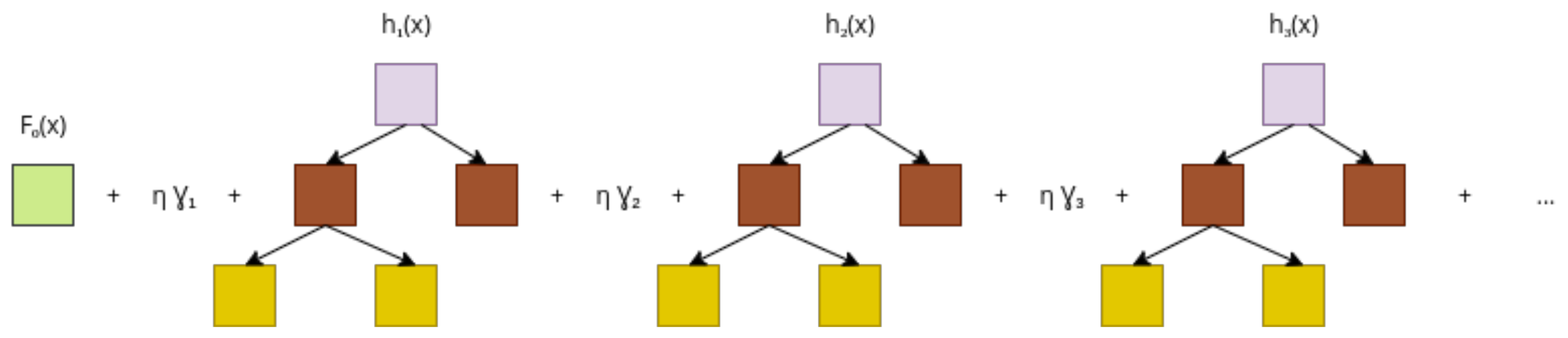
A schematic of a gradient-boosting model is shown in Figure 1. The input x is fed first into , and the result is passed down to the next tree. This procedure follows until the last tree, where the output is the precipitation. This is a constructive process, starting from the model, and a new tree is iteratively added to the model to reduce the residue.
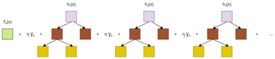
Figure 1.
Gradient-boosted trees.
An implementation of the gradient-boosting algorithm called XGBoost (eXtreme Gradient Boosting) [14] is employed here. It implements a stochastic version of the GB algorithm (SGB) [15]. XGBoost also supports regularization operators—see Equation (7). SGB allows the data samples and features to be randomly subsampled during training as an additional method to prevent overfitting. Rewriting Equation (1) with an explicit regularization operator, it becomes:
where T is the number of leaves of the tree, w are the output scores of the leaves, and and are regularization parameters. The operator can indicate -norm (), or -norm (). The -norm is related to the weaker condition for the function, where a non-differentiable function is also allowed [16,17]. A more regular (smooth) function is searched by employing the -norm [18].
Table 1 reports a description and the notation for the XGBoost hyperparameters.

Table 1.
Selected XGBoost parameters.
2.1. Best Parameters for the Gradient-Boosting Approach
Machine-learning models rely on two sets of parameters. Some parameters are inputs from the users and other ones are learned (calculated) during the training stage. The former are called hyperparameters, and the latter are called model parameters.
A model may be very sensitive to its hyperparameters, and these often require tuning. Hyperparameter tuning is a procedure to find the best combination of hyperparameters, optimizing the loss function. The optimal hyperparameters may be described as follows:
where is the set of optimal hyperparameters, P is any sample of hyperparameters, and is an objective function: the score or the loss function value of the model applied on P. A brief description of the estimated hyperparameters is shown below.
GB is a tree-based ensemble method, and one of its parameters is the tree depth (J). All the trees restricted to size J.
The learning rate () scales the contribution of each tree. It is a constant value and scales every new tree that is adjusted.
XGBoost supports both L1 and L2 regularizations and they were considered in the optimization. They are exposed in XGBoost by the reg_alpha () and reg_lambda () parameters, respectively.
Additionally, in SGB, data and features may be subsampled during training. The ratio of subsampling is exposed in XGBoost by the subsample and colsample_bytree parameters, respectively. Finally, the search space for each hyperparameter is summarized in Table 2. All other hyperparameters had their default value preserved.
Table 2.
Parameter search space.
To estimate the best hyperparameters in that search space, we used the Optuna hyperparameter optimization framework [19]. Optuna uses the Tree-structured Parzen estimators (TPE) optimization method by default [20], of sequential model-based optimization (SMBO) type, which is a sequential version of Bayesian optimization [21]. This method optimizes an objective function that returns a score, a measure of how well a particular model has performed. The score can be the mean squared error between true values and current model predicted values, as seen in Equation (10). In it, N is the number of hyperparameters in the vector P.
TPE maximizes the expected improvement (EI), as seen in Equation (11). Here, u is the hyperparameter, is the target performance, v is the loss and is a surrogate function that approximates the objective function.
TPE makes use of Bayes’ Theorem to model the surrogate function as and . The former is expressed in terms of two probability density functions and , as seen in Equation (12).
The density is formed by observations where . Conversely, the density is formed by observations where .
The “target performance” is defined in Equation (13). It represents the probability that v is under a sampled .
From it, it follows that the expected improvement is proportional to the ratio , as seen in Equation (14).
To maximize the improvement, points u should have high probability under and low probability under . On each iteration, the algorithm returns the candidate hyperparameter with the highest .
3. Methodology and Database
The dataset was originally in the NetCDF format and converted to a spreadsheet table. The entire dataset contains global data; therefore, we must extract the coordinates for our location of interest, a grid over South America. Then, the data were sorted by the coordinates. Finally, all attributes were normalized using the minimum (min) and maximum (max) normalization scheme. The general formula is given by:
where x is an original value, and is the normalized value.
3.1. GPCP Version 2.3 Precipitation Dataset
To perform climate precipitation prediction, the Global Precipitation Climatology Project (GPCP) is used as a reference dataset. It is used to train and validate the ML models.
The GPCP monthly precipitation dataset from 1979–present combines observations and satellite precipitation data into 2.5× 2.5 global grids [22]. More information about this dataset can be found at https://psl.noaa.gov/data/gridded/data.gpcp.html, accessed on 15 November 2021.
3.2. Global Meteorological Model
The general atmospheric circulation model (MCGA) of INPE is defined as the Brazilian Atmospheric Model (BAM). INPE is responsible for carrying out national numerical weather prediction every day. The center also performs the seasonal operational climate forecast. Presently, the INPE operational atmospheric circulation model for numerical forecasting of weather and climate on a global scale is the BAM [3].
In BAM’s data, the remapping of observations on grid points was performed by bilinear interpolation. The data was remapped to the same 2.5-degree GPCP resolution.
3.3. Reanalysis from the NCEP/NCAR
The meteorological variables used as initial conditions for forecasting were collected from the National Center for Environmental Prediction (NCEP) from “The Reanalysis 1” project with the National Center for Atmospheric Research (NCAR). NCEP/NCAR’s project is a state-of-the-art analysis/forecast system which has also been used to perform data assimilation using data from 1948 up to the present into a 2.5o × 2.5o global grid [23]. More details about this dataset can be found at https://psl.noaa.gov/data/gridded/data.ncep.reanalysis.surface.html, accessed on 15 November 2021.
The following meteorological variables were selected as inputs to the ML models: surface pressure, air temperature at surface, air temperature at 850 hPa, specific humidity at 850 hPa, meridional wind component at 850 hPa, zonal wind component at 500 hPa, and zonal wind component at 850 hPa.
The meteorological variables as input parameters of the ML models were chosen following a previous study, where the authors used a data science technique to identify the most significant variables for precipitation prediction [11].
3.4. Model Establishment
Machine-learning models work by making data-driven predictions or decisions from input data. This data is usually divided into multiple data sets. Typically, three sets of data are used: training, evaluation, and test sets.
Experiments were performed using a dataset from January 1980 to February 2020, with a spatial resolution of 2.5 degrees, with monthly time records. The experiments consisted of developing models for precipitation prediction over South America using two different approaches—gradient boosting, and artificial neural networks—implemented by XGBoost and TensorFlow, both of which are free software packages. The database was then divided into training, validation (evaluation), and testing subsets:
- Training and evaluation subsets were formed with data from January 1980 up to February 2017, randomly split into 75% and 25% of the set, respectively;
- The testing (prediction) subset corresponds to the period from March 2017 up to February 2020.
Consequently, the initial conditions in this work were the meteorological variables cited in Table 3: (1) surface pressure; (2) air temperature at surface; (3) air temperature at 850 hPa; (4) specific humidity at 850 hPa; (5) meridional wind component at 850 hPa; (6) zonal wind component at 500 hPa; (7) zonal wind component at 850 hPa; and (8) precipitation. The GPCP monthly precipitation was considered to be the single output, and used as a reference to evaluate the forecast obtained by the models.
Table 3.
Variables composing the dataset.
3.5. Performance Evaluation
To evaluate the performance and effectiveness of the ML algorithms (TensorFlow and XGBoost), three different evaluation metrics were selected in this study: root-mean-square error (RMSE) (Equation (16)), mean error (ME) (Equation (17)), and covariance (COV) (Equation (18)). These metrics can be calculated using the following equations:
where N is the number of entries in the dataset, denotes the target values, and is the predicted outputs.
For two variable vectors and , the covariance is defined as:
where is the mean of , is the mean of , and denotes the complex conjugate.
Error maps were calculated from the difference between the prediction models and the reanalysis values. The error map is computed by:
4. Seasonal Precipitation Prediction: Results and Discussions
The results of the climate precipitation prediction process using the machine-learning models developed in XGBoost (the XGB model) and TensorFlow (the TF model) [11,24] applied to the test dataset, for years 2018 and 2019, are presented and evaluated in this section. Precipitation maps are only shown to 2019.
The results of the forecast process using the XGB model are compared with the seasonal prediction by the numerical atmospheric model BAM and deep learning (TF model) [11].
4.1. Summer Climate Forecast
The summer season in the southern hemisphere is characterized by rising temperatures all over the continent and massive rains. In addition, in this season there are usually rapid changes in weather conditions, associated with extreme rainfall, electrical discharges related to deep convection and the development of cumulunimbus clouds with tops greater than 10 km, mainly in the south, southeast and midwest of the continent [25].
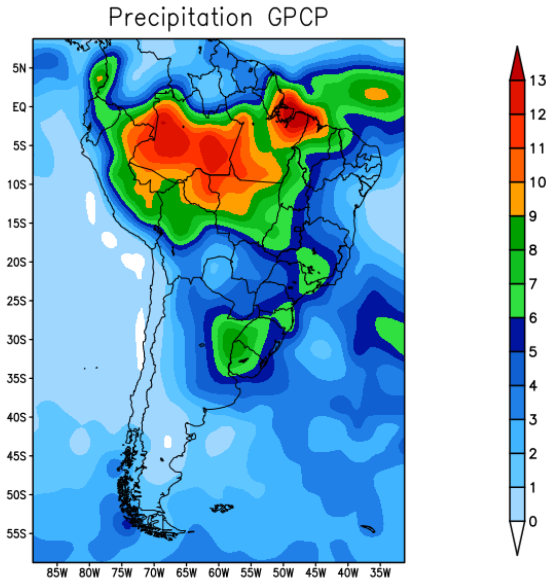
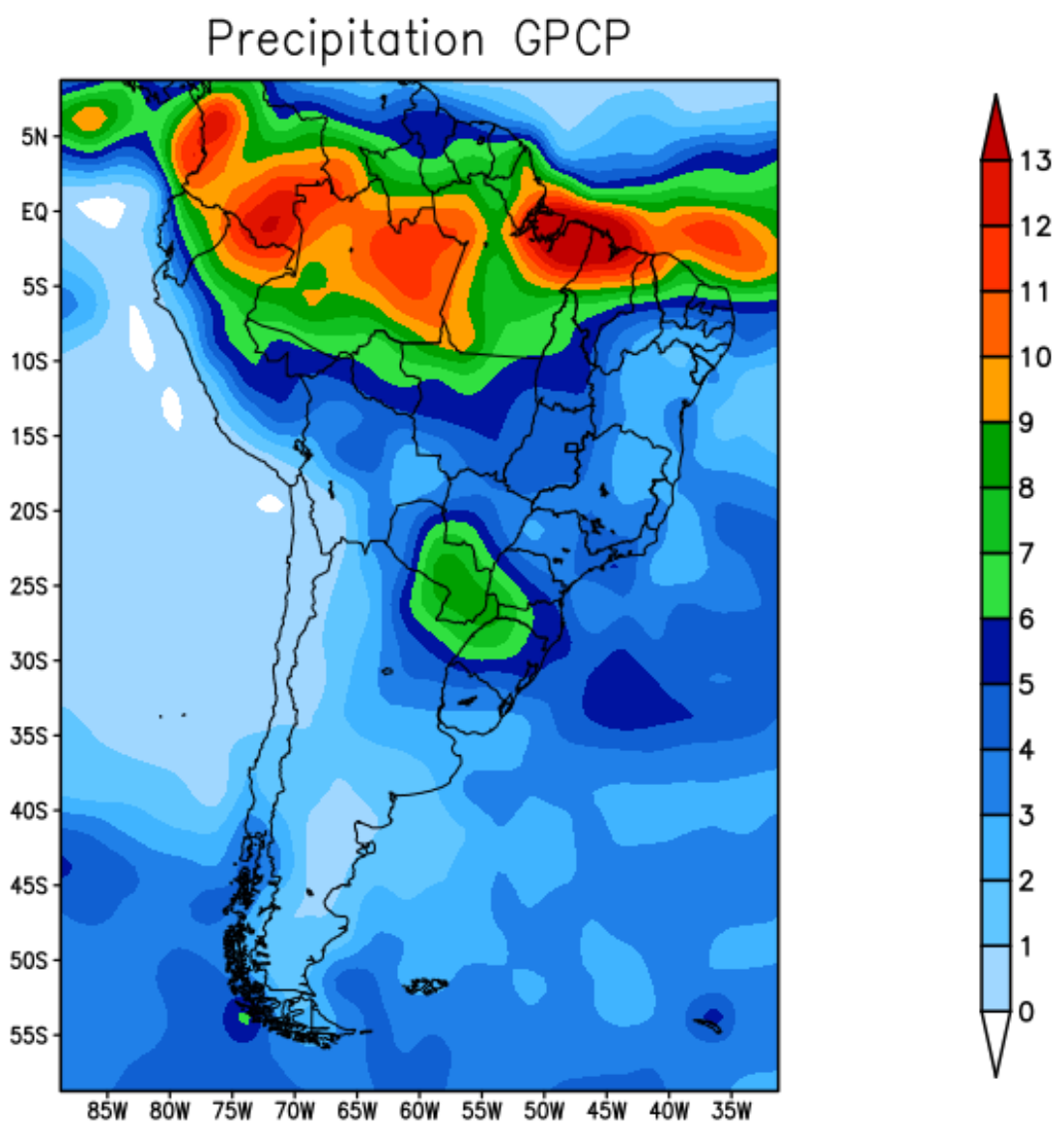
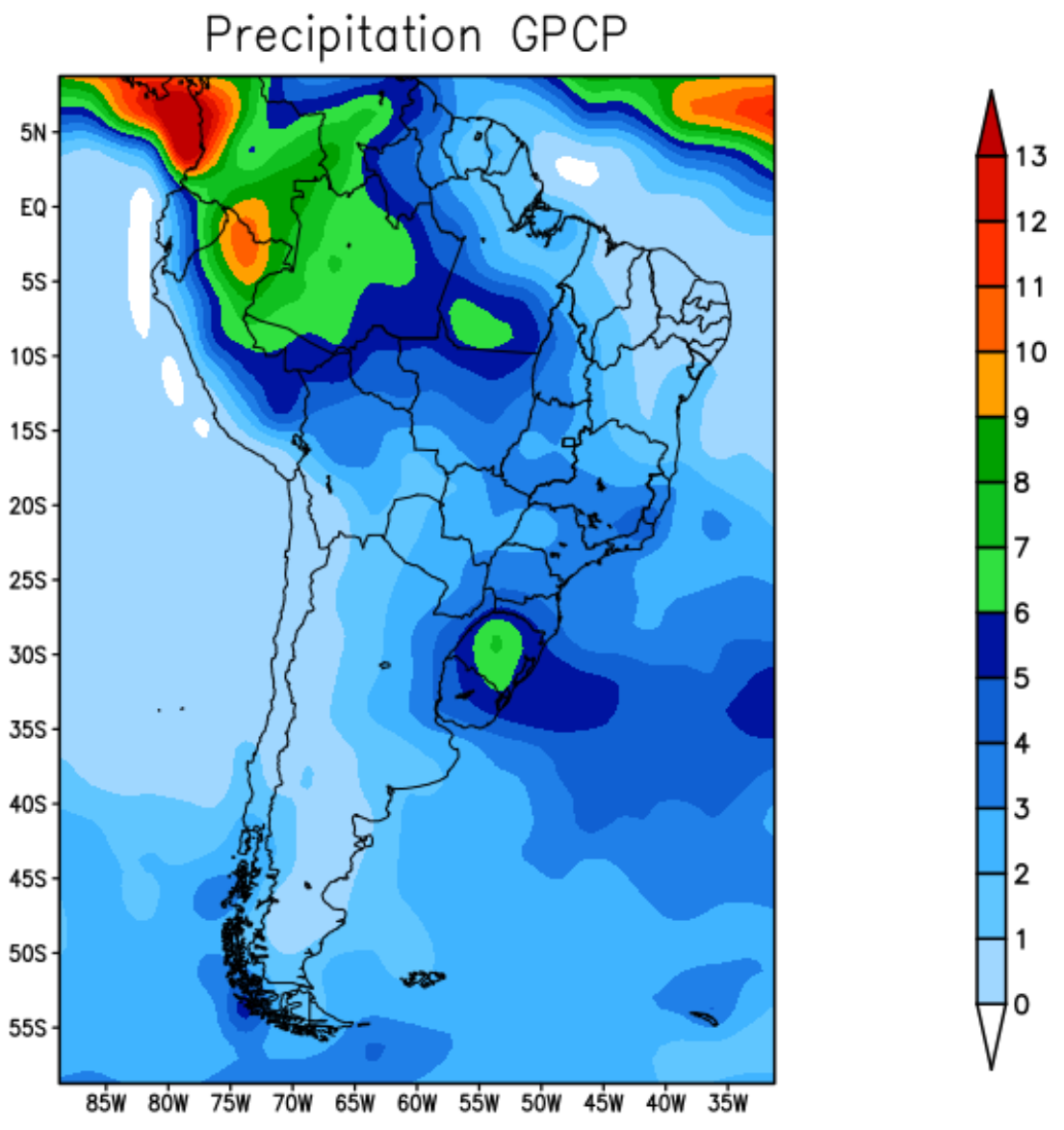
Figure 2 shows the average precipitation for the summer season December–January-February (DJF) of 2019 recorded by the GPCP. During the summer, typically the maximum amount of precipitation migrates from the central-west region of Brazil to the north of the equator. The highest rainfall rates were recorded in the north region of South American due to the southward displacement of the Intertropical Convergence Zone (ITCZ).
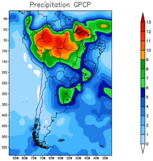
Figure 2.
GPCP precipitation—summer 2019.
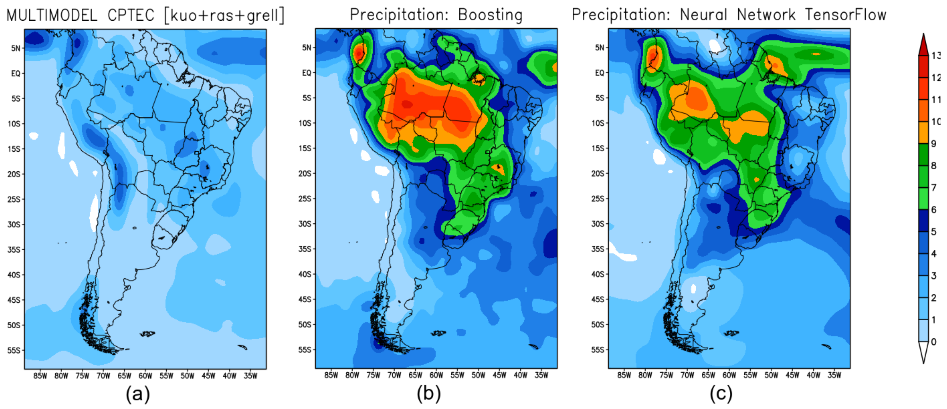
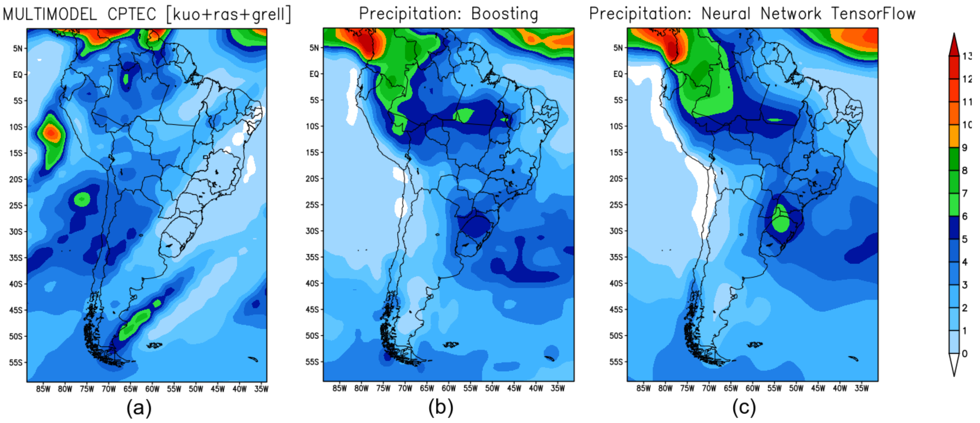
Figure 3 shows the precipitation prediction for the summer season in 2019 retrieved from the forecast models: Figure 3a shows the precipitation forecast obtained by BAM; Figure 3b shows the forecast obtained with XGB; and Figure 3c shows the prediction produced by TF.
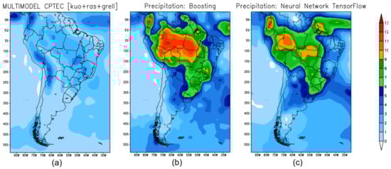
Figure 3.
Seasonal climate prediction for the summer over South America: (a) precipitation predicted by the BAM; (b) prediction by XGB; (c) prediction by TF.
Typically, in this summer season, the tropical climate (rainy season) happens on the Pacific coast of Colombia, the Amazon basin, on the coast of the Guianas and part of the coast of Brazil. The rains are intense, and well distributed. The Chocó region of Colombia is one of the rainiest areas on the entire planet, with rainfall recorded for more than 300 days a year—see Figure 2 which shows the region with a high record of rainfall observed.
XGB-(Figure 3b) and TF-(Figure 3c) models identify precipitation maximums in the coastal region of Colombia, Peru, and the Amazon region of Brazil. In the southeast region of Brazil, the three models were not able to accurately predict compared to what was observed.
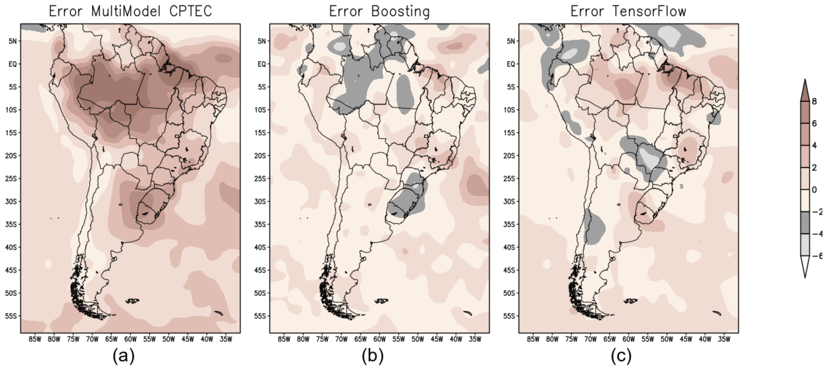
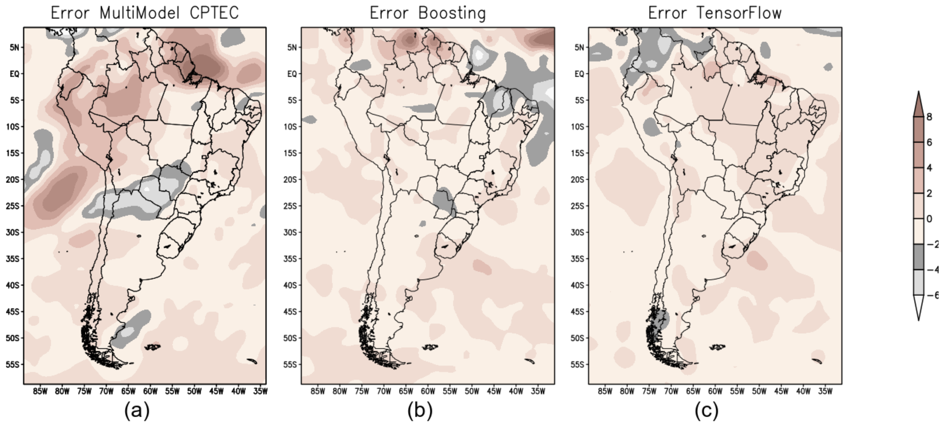
Figure 4 shows the error map (mm/day) calculated from the difference between the observed precipitation (GPCP) and the prediction produced by the three models—BAM (Figure 4a); XGB (Figure 4b); and TF (Figure 4c).
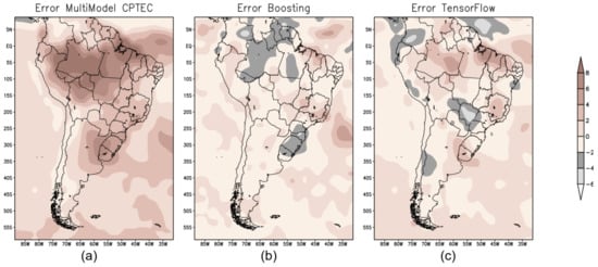
Figure 4.
Error map to evaluate the performance of the forecast models: (a) BAM; (b) XGB; and (c) TF.
For the forecast for the summer season over South America, both ML models showed better results compared to the numerical model BAM; see error map (Figure 4b,c ).
4.2. Autumn Climate Forecast
The autumn season in the southern hemisphere is considered a transition season between summer and winter. In this season, the winds increase and gradually grow stronger. In addition, as autumn precedes winter, temperatures usually decrease and consequently the air humidity decreases. In the northern part of the northeast and north regions of Brazil, it is still a time of heavy rain, especially if the ITCZ persists further south of its climatological position [26].
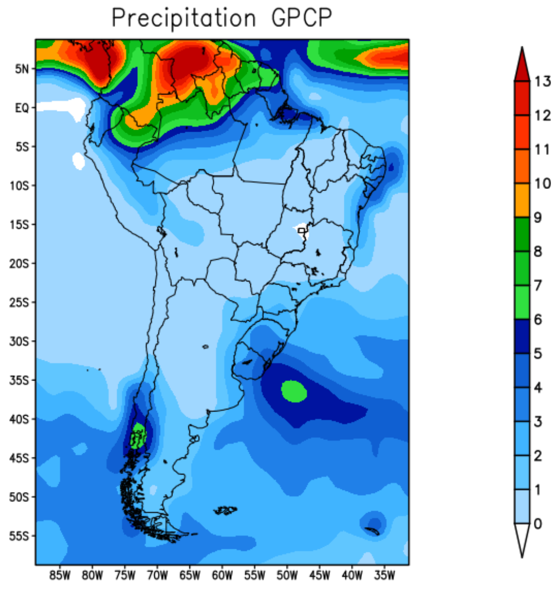
Figure 5 shows the observed GPCP precipitation field for the autumn season March-April-May (MAM). The maximum precipitation amounts are related to the southward displacement of the ITCZ, which is very active near the north coast of South America. The charged clouds advance from the sea and enter the interior of northeastern Brazil, causing storms [27].
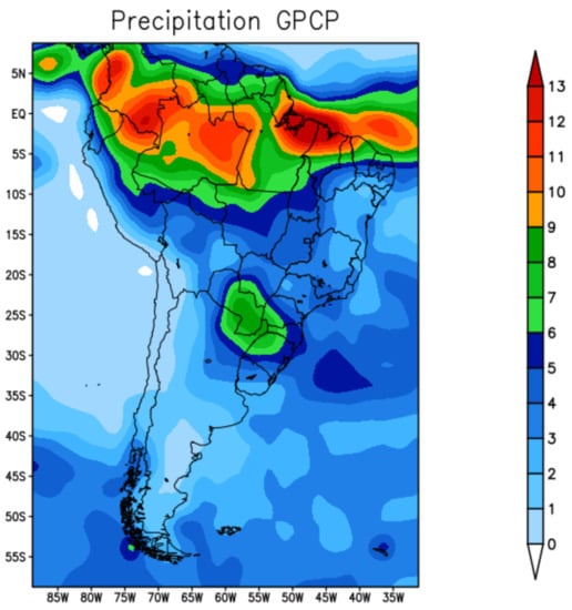
Figure 5.
GPCP precipitation—autumn 2019.
Figure 6 shows the precipitation prediction for the autumn in 2019 retrieved from the forecast models: BAM (Figure 6a); XGB (Figure 6b); and TF (Figure 6c).
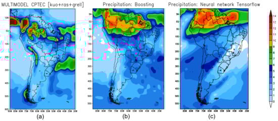
Figure 6.
Seasonal climate prediction for the autumn 2019 in South America: (a) precipitation predicted by BAM; (b) precipitation predicted by XGB; (c) prediction obtained by TF.
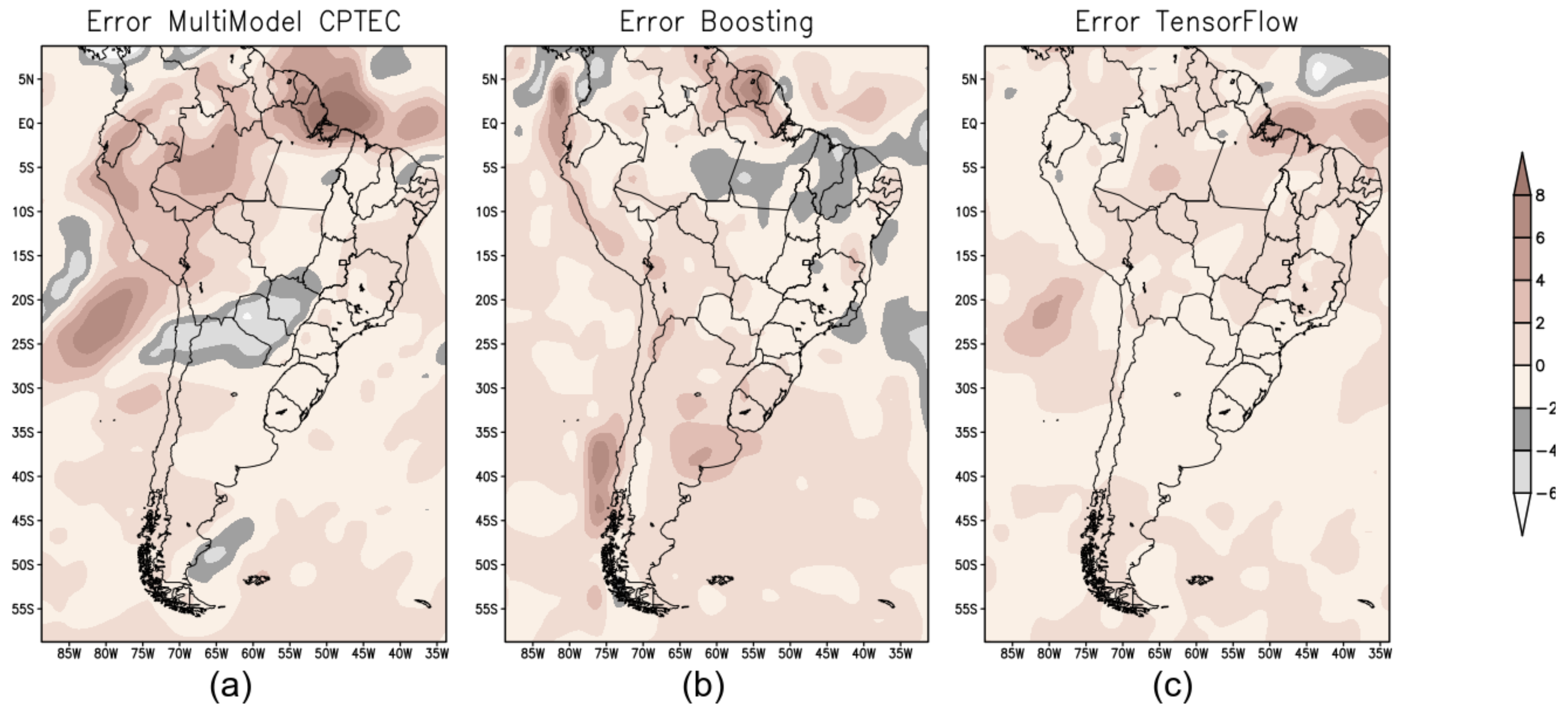
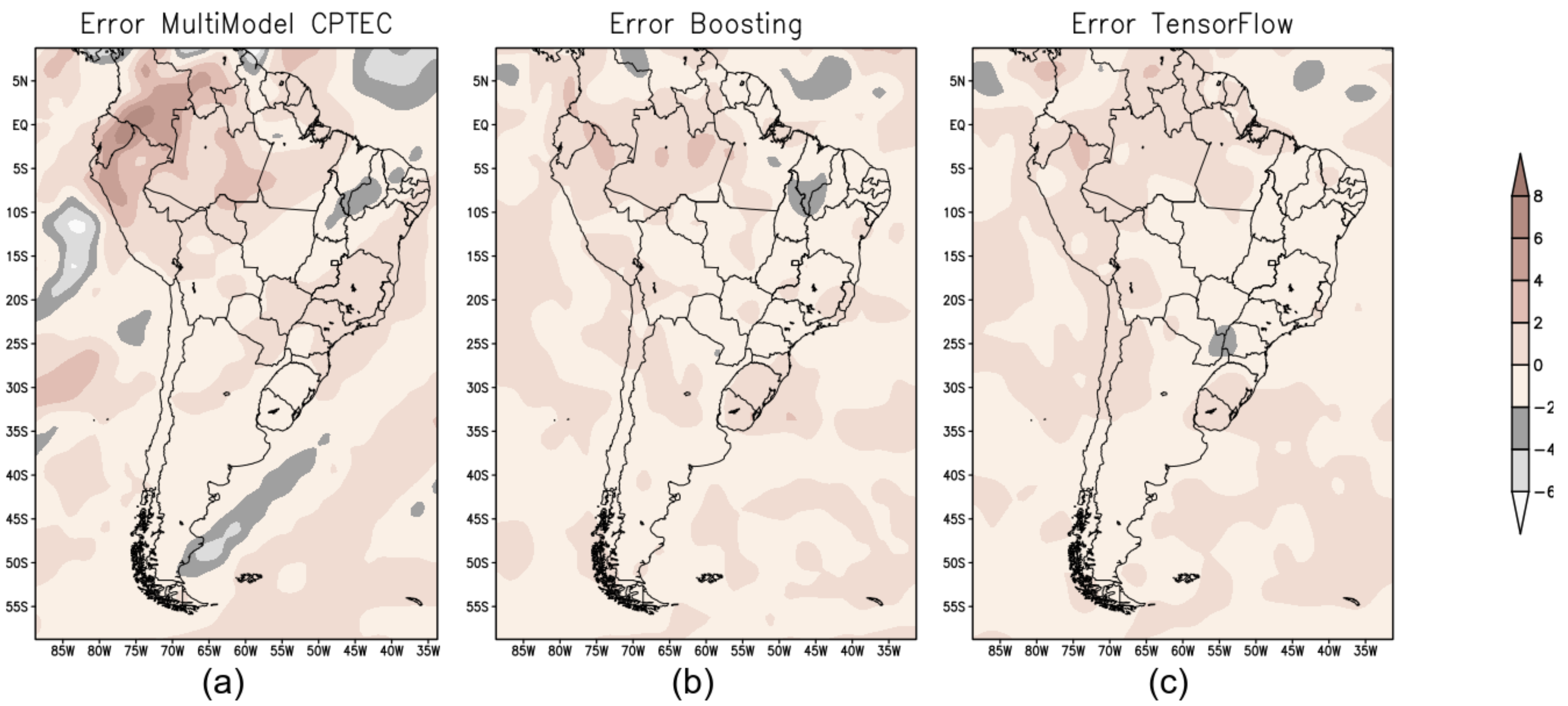
Figure 7a shows the error map (mm/day) calculated from the difference between the observed precipitation (GPCP) and the numerical prediction by the BAM; Figure 7b shows the error map for the XGB; and Figure 7c represents the error map for TF.
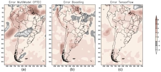
Figure 7.
Error map for the autumn in South America to evaluate the performance of the forecast models: (a) BAM; (b) XGB; and (c) TF.
XGB and TF reproduced the most significant precipitation recorded in the GPCP data. These extreme precipitations were observed in Colombia, Ecuador, Peru, Venezuela, and in Brazil in the states of Amazonas, Roraima, Pará, Maranhão and Ceará—see Figure 6b,c.
4.3. Winter Climate Forecast
The winter season in the southern hemisphere is characterized by decreasing temperatures and humidity. However, the drop in temperature records is not as great as in the northern hemisphere. This area has a temperate climate, which generally presents heavy rainfall in the northern region of Brazil, influenced by the position of the ITCZ. However, countries located in higher latitudes, such as Argentina and Chile have a more rigorous winter, due to the influence of temperate and polar zones, marked by the record of negative temperatures and also by the occurrence of snow precipitation [28].
Figure 8 represents the GPCP precipitation for the winter season—June–July–August (JJA) and Figure 9 shows the precipitation prediction for the winter season in 2019 produced from the forecast models: BAM (Figure 9a); XGB (Figure 9b); and TF (Figure 9c).
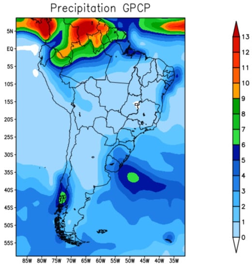
Figure 8.
GPCP precipitation—winter 2019.
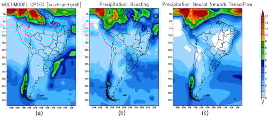
Figure 9.
Seasonal climate prediction for winter in South America: (a) precipitation predicted by BAM; (b) prediction obtained by XGB; (c) precipitation prediction obtained using TF.
Figure 10 shows the error map (mm/day) of the forecast calculated from the difference between the GPCP precipitation and the forecast obtained by the models—BAM (Figure 10a); XGB (Figure 10b); and TF (Figure 10c).
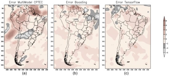
Figure 10.
Error map for winter in South America to evaluate the performance of the forecast models: (a) BAM; (b) XGB; and (c) TF.
The maximum precipitation values located in the extreme north of South America are related to the southward displacement of the Intertropical Convergence Zone (ITCZ). ITCZ. According to the precipitation prediction results made by the three models, it is noted that all models can predict precipitation in the extreme north. However, it is evident that the best result was obtained by TF—see Figure 9c—and the error map shows that it was the only one that produced the forecast reproducing the precipitation observed in the GPCP—see Figure 10c.
4.4. Spring Climate Forecast
In the spring in the southern hemisphere, the southern oceans are still cold and are gradually warming up. This season is a transition period between the dry and wet seasons in central Brazil, as well as the beginning of the Amazon moisture convergence, which defines the quality of the rainy season in the midwest, southeast and midsouth regions, and part of the northern region [29].
Figure 11 represents the observed precipitation for the spring season September-October-November (SON). Figure 12 shows the precipitation climate prediction for the spring season in 2019 obtained by the models: BAM (Figure 12a); XGB (Figure 12b); and TensorFlow (Figure 12c). XGB and TF reproduced the most significant precipitation cores that occurred in Colombia, northern Peru, Venezuela and the Brazilian state of Amazonas—see Figure 12b,c.
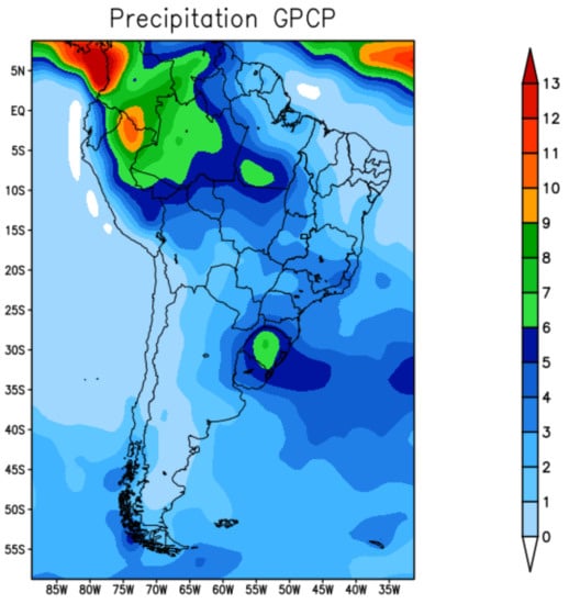
Figure 11.
GPCP precipitation—spring 2019.
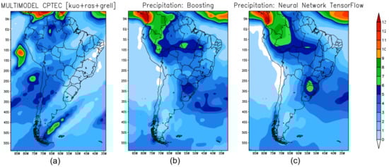
Figure 12.
Seasonal climate forecast for spring in South America: (a) precipitation predicted by BAM model; (b) prediction obtained by XGBoost model; (c) prediction obtained by TF.
Figure 13 shows the error map of the forecast for spring season produced by the three models—BAM (Figure 13a); XGB (Figure 13b); and TF (Figure 13c).
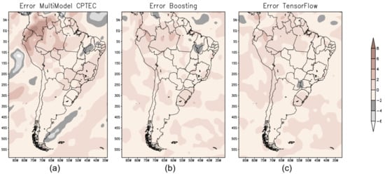
Figure 13.
Error map for spring in South America to evaluate the performance of the forecast models: (a) error map produced from the difference between the GPCP precipitation dataset and the precipitation prediction by BAM; (b) error map for XGB; and (c) error map for TF.
4.5. Evaluation Performance of Models and Discussions
After the optimization process, the best hyperparameters obtained for XGB were saved, and they are shown in Table 4. A different model was trained for each season; hence there are four different columns of hyperparameters in it.
Table 4.
Best parameters for each season.
As mentioned in Section 3.5, the quantitative performance evaluation metrics for the machine-learning models were the root-mean-square error (RMSE), mean error (ME), and covariance (COV).
Table 5 shows the numerical results to evaluate the performance of the proposed ML models for precipitation prediction in the years 2018 and 2019, respectively. For 2018, XGB presented a better performance for summer, winter, and spring seasons, while TF was better for the autumn season. Analyzing the evaluation parameters obtained for 2019, XGB presented a better performance for summer and spring seasons, and TF was better for autumn and winter seasons. However, the difference between XGB and TF is not so significant to the RMSE values; the greater difference is noted for the covariance—see Table 5.
Table 5.
Performance evaluation for XGB and TF model.
The comparison between atmospheric dynamics prediction model BAM and TF for climate precipitation prediction over South America has already been executed by Anochi and co-authors [11]. In the present paper, we point out the numerical performance between TF and XGB.
Intense rainfall events in South America are also related to the Intertropical Convergence Zone (ITCZ) [30] and South Atlantic Convergence Zone (SACZ) [31]. The ITCZ is noted as a band of clouds linked to thunderstorms in general. The phenomena occur in the equatorial zone, for both hemispheres. The ITCZ is explained as a signature of the Hadley cell with wet air. An ITCZ thunderstorm was associated with the loss of Air France Flight 447, from Rio de Janeiro (Galeão airport) on 31 May 2009. The aircraft crashed during flight with no survivors. SACZ is characterized by an elongated strip of clouds oriented in a northwest-southeast manner across southeast Brazil into the southwest Atlantic Ocean. More intense thunderstorms are verified when the Madden–Julian oscillation passes into the region. The rains caused by the SACZ were responsible for the floods and landslides in the state of Rio de Janeiro (Brazil) in 2011, with more than 900 fatalities.
The ITCZ and SACZ are strongest in the warm season in South America—spring and summer. During summer 2019, XGB had a better prediction for this condition than TF—see Figure 3. For this year, a wetter season was verified during the autumn, and TF presented better forecasting. From our results, TF was more effective to identify the climate pattern for the autumn than the BAM and XGB predictions.
5. Conclusions and Final Remarks
The gradient-boosting framework XGBoost [14] was used as the predictor tool for seasonal climate precipitation over South America. Wang and co-authors [32] used an ensemble of several ML algorithms with different configurations as the model tool for load forecast [32] and, among the algorithms, the gradient-boosting technique was evaluated too. Another strategy was used here to design the ML predictor. The best parameters to improve the performance of the XGB model was determined by a Bayesian optimization scheme codified in the Optuna framework [19].
As already known, the precipitation process is not well represented by physical parametrizations in the numerical models for weather and climate predictions [9]. Our results, in some sense, agree with other studies for comparison with numerical codes and machine-learning prediction tools—see for example [9]. For pattern recognition for precipitation, XGB configured by the Optuna optimizer presented a better result than the TF deep neural network for summer, winter, and spring, while TF has a better performance for autumn for the two years during the test of hindcasting experiments. An additional study deserves to be developed to define which meteorological pattern was not well identified during the autumn season by XGB. Probably a hidden pattern better identified by the deep network could emerge by inserting another attribute as a new input for XGB.
A database for the period of years from 1980 up to 2020 was used for training and testing the supervised XGB estimator, with the period March 2017 up to February 2020 being selected to evaluate the forecasting performance of the gradient-boosting procedure adopted. The results were compared with the prediction carried out by the TF and BAM models. For 2018, XGB presented better performance for summer, winter, and spring seasons, while TF was better for autumn. The next year, 2019, better results were obtained by XGB for summer and spring, with TF showing better performance for autumn and winter. However, the difference between XGB and TF is not so significant considering the RMSE values, although a greater difference is noted for the covariance—see Table 5.
Overall, XGB had better results than TF. However, as there is no superior prediction technique for all seasons. One recommendation would be to use both techniques in combination.
Author Contributions
Conceptualization: V.S.M.; J.A.A. and H.F.d.C.V.; Software adaptation: V.S.M.; Validation: V.S.M. and J.A.A.; Writing—original draft preparation: V.S.M.; J.A.A. and H.F.d.C.V.; Writing—review and editing: V.S.M., J.A.A. and H.F.d.C.V. All authors have read and agreed to the published version of the manuscript.
Funding
This research received no external funding.
Institutional Review Board Statement
Not applicable.
Informed Consent Statement
Not applicable.
Data Availability Statement
This paper used free dataset available upon request.
Acknowledgments
Authors wish to thank the National Institute for Space Research. Author VSM thanks the Coordination for the Improvement of Higher Education Personnel (CAPES, Brazil), and author HFCV also thanks the National Council for Scientific and Technological Development (CNPq, Brazil) for the research grant (CNPq: 312924/2017-8).
Conflicts of Interest
The authors declare no conflict of interest.
References
- Iseh, A.; Woma, T. Weather Forecasting Models, Methods and Applications. Int. J. Eng. Res. Technol. 2013, 2, 1945–1956. [Google Scholar]
- Lorenz, E.N. Deterministic Nonperiodic Flow. J. Atmos. Sci. 1963, 20, 130–141. [Google Scholar] [CrossRef] [Green Version]
- Figueroa, S.N.; Bonatti, J.P.; Kubota, P.Y.; Grell, G.A.; Morrison, H.; Barros, S.R.; Fernandez, J.P.; Ramirez, E.; Siqueira, L.; Luzia, G.; et al. The Brazilian global atmospheric model (BAM): Performance for tropical rainfall forecasting and sensitivity to convective scheme and horizontal resolution. Weather Forecast. 2016, 31, 1547–1572. [Google Scholar]
- Lagerquist, R.; McGovern, A.; Gagne, D.J., II. Deep Learning for Spatially Explicit Prediction of Synoptic-Scale Fronts. Weather Forecast. 2019, 34, 1137–1160. [Google Scholar] [CrossRef]
- Ham, Y.G.; Kim, J.-H.; Luo, J.J. Deep learning for multi-year ENSO forecasts. Nature 2019, 573, 568–572. [Google Scholar] [CrossRef]
- Schultz, M.G.; Betancourt, C.; Gong, B.; Kleinert, F.; Langguth, M.; Leufen, L.H.; Mozaffari, A.; Stadtler, S. Can Deep Learning Beat Numerical Weather Prediction? Philos. Trans. Royal Soc. A Math. Phys. Eng. Sci. 2021, 379, 20200097. [Google Scholar] [CrossRef]
- Agata, R.; Jaya, I.G.N.M. A comparison of extreme gradient boosting, SARIMA, exponential smoothing, and neural network models for forecasting rainfall data. J. Phys. Conf. Ser. 2019, 1397, 012073. [Google Scholar] [CrossRef]
- Cui, Z.; Qing, X.; Chai, H.; Yang, S.; Zhu, Y.; Wang, F. Real-time rainfall-runoff prediction using light gradient boosting machine coupled with singular spectrum analysis. J. Hydrol. 2021, 603, 127124. [Google Scholar] [CrossRef]
- Ukkonen, P.; Makela, A. Evaluation of Machine Learning Classifiers for Predicting Deep Convection. J. Adv. Model. Earth Syst. 2019, 11, 1784–1802. [Google Scholar] [CrossRef] [Green Version]
- Freitas, J.H.V.; França, G.B.; Menezes, W.F. Deep convection forecasting using decision tree in Rio de Janeiro metropolitan area. Anuário do Inst. de Geociências (UFRJ. Brazil) 2019, 42, 127–134. [Google Scholar]
- Anochi, J.A.; de Almeida, V.A.; de Campos Velho, H.F. Machine Learning for Climate Precipitation Prediction Modeling over South America. Remote Sens. 2021, 13, 2468. [Google Scholar] [CrossRef]
- Friedman, J.H. Greedy Function Approximation: A Gradient Boosting Machine. Ann. Stat. 2001, 29. [Google Scholar] [CrossRef]
- Bentéjac, C.; Csörgo, A.; Martínez-Muñoz, G. A Comparative Analysis of XGBoost. arXiv 2019, arXiv:abs/1911.01914. [Google Scholar]
- Chen, T.; Guestrin, C. XGBoost: A Scalable Tree Boosting System. In Proceedings of the 22nd ACM SIGKDD International Conference on Knowledge Discovery and Data Mining, San Francisco, CA, USA, 13–17 August 2016; ACM: New York, NY, USA; pp. 785–794. [Google Scholar] [CrossRef] [Green Version]
- Friedman, J.H. Stochastic gradient boosting. Comput. Stat. Data Anal. 2002, 38, 367–378. [Google Scholar] [CrossRef]
- Rudin, L.I.; Osher, S.; Fatemi, E. Nonlinear Total Variation Based Noise Removal Algorithms. Phys. D Nonlinear Phenoma 1992, 60, 259–268. [Google Scholar]
- Aster, R.C.; Borchers, B.; Thurber, C.H. Parameter Estimation and Inverse Problems; Elsevier: Amsterdam, The Netherlands, 2018. [Google Scholar]
- Tikhonov, A.N.; Arsenin, V.Y. Solution of Ill-Posed Problems; John Wiley & Sons: Hoboken, NJ, USA, 1977. [Google Scholar]
- Akiba, T.; Sano, S.; Yanase, T.; Ohta, T.; Koyama, M. Optuna: A Next-Generation Hyperparameter Optimization Framework. arXiv 2019, arXiv:cs.LG/1907.10902. [Google Scholar]
- Bergstra, J.; Bardenet, R.; Bengio, Y.; Kégl, B. Algorithms for Hyper-Parameter Optimization. In Advances in Neural Information Processing Systems 24: Proceedings of the 25th Annual Conference on Neural Information Processing Systems 2011, Granada, Spain, 12–14 December 2011; Curran Associates Inc.: New York, NY, USA, 2011; pp. 2546–2554. [Google Scholar]
- Frazier, P.I. A Tutorial on Bayesian Optimization. arXiv 2018, arXiv:abs/1807.02811. [Google Scholar]
- Adler, R.F.; Huffman, G.J.; Chang, A.; Ferraro, R.; Xie, P.P.; Janowiak, J.; Rudolf, B.; Schneider, U.; Curtis, S.; Bolvin, D.; et al. The Version-2 Global Precipitation Climatology Project (GPCP) Monthly Precipitation Analysis (1979–present). J. Hydrometeorol. 2003, 4, 1147–1167. [Google Scholar] [CrossRef]
- Kalnay, E.; Kanamitsu, M.; Kistler, R.; Collins, W.; Deaven, D.; Gandin, L.; Iredell, M.; Saha, S.; White, G.; Woollen, J.; et al. The NCEP/NCAR 40-year reanalysis project. Bull. Am. Meteorol. Soc. 1996, 77, 437–472. [Google Scholar]
- Abadi, M.; Agarwal, A.; Barham, P.; Brevdo, E.; Chen, Z.; Citro, C.; Corrado, G.; Davis, A.; Dean, J.; Devin, M.; et al. TensorFlow: Large-Scale Machine Learning on Heterogeneous Distributed Systems. 2016. Available online: http://xxx.lanl.gov/abs/1603.04467 (accessed on 27 December 2021).
- Summer Climate Forecast. Available online: https://portal.inmet.gov.br/notasTecnicas# (accessed on 28 December 2021).
- Autumn Climate Forecast. Available online: https://portal.inmet.gov.br/notasTecnicas# (accessed on 28 December 2021).
- Ferreira, N.S. Intertropical Convergence Zone. Climanalysis Spec. Bull. 10 Years Celebr. 1996, 10, 15–16. [Google Scholar]
- Newman, P.A.; Nash, E.R. The unusual Southern Hemisphere stratosphere winter of 2002. J. Atmos. Sci. 2005, 62, 614–628. [Google Scholar]
- Prognóstico Climático de Primavera. Available online: https://portal.inmet.gov.br/notasTecnicas# (accessed on 28 December 2021).
- Barry, R.G.; Chorley, R.J. Atmosphere, Weather, and Climate; Routledge: London, UK, 1992. [Google Scholar]
- Carvalho, L.M.V.; Jones, C.; Leibman, B. The South Atlantic Convergence Zone: Intensity, Form, Persistence, and Relationships with Intraseasonal to Interannual Activity and Extreme Rainfall. J. Clim. 2004, 17, 88–108. [Google Scholar] [CrossRef] [Green Version]
- Wang, Y.; Zhang, N.; Tan, Y.; Hong, T.; Kirschen, D.S.; Kang, C. Combining probabilistic load forecasts. IEEE Trans. Smart Grid 2019, 10, 3664–3674. [Google Scholar] [CrossRef] [Green Version]


Publisher’s Note: MDPI stays neutral with regard to jurisdictional claims in published maps and institutional affiliations. |
© 2022 by the authors. Licensee MDPI, Basel, Switzerland. This article is an open access article distributed under the terms and conditions of the Creative Commons Attribution (CC BY) license (https://creativecommons.org/licenses/by/4.0/).