Simulation of Arctic Thin Ice Clouds with Canadian Regional Climate Model Version 6: Verification against CloudSat-CALIPSO

Abstract

Polar clouds are, as a consequence of the paucity of in situ observations, poorly understood compared to their lower latitude analogs, yet highly climate-sensitive through thermal radiation emission. The prevalence of Thin Ice Clouds (TIC) dominates in cold Polar Regions and the Upper Troposphere Lower Stratosphere (UTLS) altitudes. They can be grouped into 2 broad categories. The first thin ice cloud type (TIC1) is made up of high concentrations of small, non-precipitating ice crystals. The second type (TIC2) is composed of relatively small concentrations of larger, precipitating ice crystals. In this study, we investigate the ability of a developmental version of the Canadian Regional Climate Model (CRCM6) in simulating cold polar-night clouds over the Arctic Ocean, a remote region that is critical to atmospheric circulation reaching out to the mid-latitudes. The results show that, relative to CloudSat-CALIPSO vertical profile products, CRCM6 simulates high-latitude and low spatial frequency variations of Ice Water Content (IWC), effective radius (re) and cooling rates reasonably well with only small to moderate wet and dry biases. The model can also simulate cloud type, location, and temporal occurrence effectively. As well, it successfully simulated higher altitude TIC1 clouds whose small size evaded CloudSat detection while being visible to CALIPSO.

1. Introduction

The Arctic is one of the most climate-sensitive regions on Earth [1]. Surface observations demonstrate a warming trend over the 1954–2003 climate period and still increasing to this date, especially in continental areas during winter with some cool anomalies predominantly oceanic areas, such as southern Greenland. Most climate model projections concur regarding the continuation of this strong Arctic warming trend (e.g., [2,3,4,5,6]). For instance, Camiso using the Advanced Very High-Resolution Radiometer (AVHRR) thermal infrared satellite data studied the seasonal trend in land and water surface temperature during cloud-free conditions over the period of 1981 to 2012. He found mainly positive surface temperature trends in summer, spring, and autumn broadly over the Arctic Ocean associated with sea ice retreats, but noted some negative trends during the winter, with some cooling observed over large areas of the Bering Sea and parts of Russia. These cold-season cooling anomalies were shown to be sensitive to thin ice cloud formation and atmospheric dehydration [7]. They are notable since they may affect climate variability, atmospheric circulation, and, potentially, the genesis of winter storms.

The Arctic energy balance and climate are highly sensitive to disturbances in cloud microphysical properties [6,8], sea-ice cover, and greenhouse gases, especially water vapor at low concentrations. This is particularly the case for optically thin ice clouds where the spectral emissivity and their cooling rates through the amplitude of the transmittance Jacobian [9] are shown to vary drastically as a function of crystal size and ice water content. This is particularly the case during the cold season when TIC prevails. The current study is an essential step in our ongoing investigation of the perturbative effect of optically thin polar clouds, with optical depth ($\tau$) less than 3, on the generation of available potential energy affecting mid-latitude synoptic storm during winter and spring.

The ability of climate models to simulate feedbacks between different components of the climate system depends, to a significant extent, on how well processes governing regional high-latitude dynamics are integrated into the models. Cloud-radiation feedbacks are, due to functional dependencies and interactions between various components of the system (in particular, clouds, sea ice, and snow cover), extremely complex in the Arctic (notably the feedback relationship between Arctic clouds and surface air flows). Sea ice and surface temperatures are strongly influenced by clouds: their presence can indirectly affect atmospheric temperatures, air dehydration, boundary layer stability, sensible heat fluxes, and other derived variables [6,10]). Cloud optical thickness, altitude, microphysics, and cloud cover can also be influenced by changes in atmospheric temperature and static stability (thus adding to the intricate web of feedbacks). Globally, clouds produce net surface heating by virtue of the infrared radiation they emit [11]. Thin clouds also exert a substantial net atmospheric cooling effect during the Arctic night. They act as a three-dimensional radiator of thermal radiation in the volume of the atmosphere that contains [11]. As semi-transparent grey bodies, they act as efficient three-dimensional radiators of thermal radiation within the atmospheric volume that they occupy. In contrast, optically thick, low-altitude clouds cool approximately like black bodies at their upward-looking boundaries while generally warming the air at their bases due to upwelling warm surface radiation in the case of a sunlit surface or warm ocean water. During the warm season, low-level, mixed-phase polar clouds have a net cooling effect that is brought about by the reduction of solar radiation at the surface: however, they exert compensatory infrared effects due to the enhanced greenhouse effect [11,12]. Thermal surface cooling by infrared radiation during the polar night also promotes the ubiquitous Arctic temperature inversion layer including over arctic sea ice [13,14] and generates extremely stable conditions at low altitudes. These long polar-winter periods of stable boundary layer conditions alternate with summertime periods of weakly stable or near-neutral heating conditions driven by the influence of wind, heat advection from low latitudes, and radiation [15,16].

One ongoing problem with Arctic climate simulations is the scarcity of long-term observation sites that can be employed for characterizing regional-scale climate and for evaluating high-resolution models. Indeed, most cloud microphysical data are taken during special measurement campaigns. Another source of data is the network of polar-orbiting satellites, particularly the A-Train constellation that includes (or included at the time of our observations) OCO-2, GCOM-W1, Aqua, Aura, CloudSat, and CALIPSO. CALIPSO and MODIS-Aqua as well as MODIS-TERRA have provided considerable data over the last two decades [17,18]. Most passive instruments such as the MODIS imaging spectroradiometers have difficulty distinguishing cloud-top and icy-surface radiation due to low-level Arctic inversions as well as similarities in the optical properties of clouds and snow. The CloudSat cloud probing radar (CPR) and the CALIPSO Cloud-Aerosol Lidar with Orthogonal Polarization (CALIOP) are active instruments that have, since 2006, transformatively improved the regularity and spatial extent of aerosol and cloud vertical-structure profiling.

The results of a variety of measurement campaigns indicate or suggest the presence of various types of imperfections in Arctic climate models [10]. Such imperfections can result from oversimplified parametrizations that inadequately represent atmospheric processes in the Arctic. In most models, the radiation balance of, for example, thin ice clouds (TICs), ubiquitous diamond dust precipitation, and Arctic haze are not well represented [19,20]. Comparing model simulations with satellite data allows model biases to be evaluated while enabling a better understanding of physical and microphysical processes in the Arctic atmosphere.

Arctic-warming effects have been more thoroughly studied over land areas because there are no permanent observing oceanic stations. Satellite observations show strong warming variation over the Arctic Ocean [4,6]: sectors that tend to be warming also show warming variations and trends that are highly variable. The extent of the dependency of the variation on cloud properties, notably the effects of those cloud properties on the energy balance as well as on atmospheric circulation remains uncertain, especially at high latitudes. Indeed, cloud feedback has been recognized as a major source of uncertainty in climate projections [21]. Clouds play a dominant role in regulating the atmospheric radiation budget by influencing both solar radiation and infrared radiation. They also play a role in the modulation of the hydrological cycles through the agency of cloud processes and precipitation formation that can have a controlling influence on the water balance of the atmosphere.

The climatology of polar clouds, as reported in the literature, can differ considerably as a function of the observing periods, cloud types, and data sources. Shupe et al. [22] employed ground-based remote sensing measurements to estimate the average cloud fraction over a limited number of Arctic sites (Barrow and Atqasuk, AK, U.S.; Eureka, NU, Canada; Ny-Ålesund, Spitsbergen, Norway; and Summit, Greenland, Denmark) was 58% in winter and 83% in summer. Additional Supplementary Data were acquired during 1997–1998 (September to September) SHEBA (Surface Heat Budget of the Arctic Ocean) campaign [16,23]. Shupe [22,24] showed that the surface radiative balance in the Arctic strongly depends upon the presence of clouds. However, these statistics predated the advent of the CloudSat and CALIPSO missions and only accounted for optically thick clouds. Curry et al. [10] compared a number of studies and concluded that the average Arctic-winter cloud fraction typically ranges from 40 to 68% (increasing to 80% during clear sky ice-crystal precipitation events if TICs were considered). The Arctic climate effect of thin ice clouds, particularly on the energy cycle and atmospheric circulation, has, however, yet to be quantified. One way to achieve this quantification is to perform a rigorous energy budget calculation based on the conservative equations of field dynamics and thermodynamics that are used in numerical forecast models [25]. However, to achieve this objective, it is essential to verify that the atmospheric model can adequately simulate TICs when driven by realistic boundaries during intensive measurement periods, such as the International Polar Year (2007–2008). It is equally essential to assess the limitations of the model for the analysis. It is the purpose of this paper.

An important legacy of the 15 years of satellite-based LiDAR and radar data acquired to date, is that during the polar night, TICs are known to be dominant over the High Arctic. These very cold and semi-transparent clouds emit longwave radiation, not only from their boundaries but within their large cloud volume, depleting thermal energy very effectively from their large cloud volume rather than only from their edges. This is unlike any phenomenon observed in warm, low-latitude regions. One effect of this dominant, cold-season radiative cooling process is to strengthen the polar vortex, thereby increasing geopotential gradients, enhancing the jet stream and, ultimately, leading to intensification of mid-latitude storm activity. Then, radiation is highly sensitive to cloud microphysics, particularly to cloud phase, ice crystal size, number concentration, and cloud optical depth. In such conditions, radiation transmittance and cloud emissivity exhibit strong variation, modulating the longwave radiative cooling rate and the energy balance at broad regional scales. Apart from this direct effect of cloud microphysics on radiation, an indirect effect takes place through precipitation, dehydration, and greenhouse, called Dehydration-Greenhouse Feedback (DGF) effect [26]. Previous studies [27,28,29,30] have shown that DGF dependency on cloud microphysics and ice crystal precipitation is largely controlled by nucleation processes, especially under the influence of pollution-related acidification of ice nuclei in a cold-dry environment, such as Arctic haze of volcanic plumes.

Previous studies [27,28,29,30,31] distinguished two types of TICS: the TIC1 type consists of high concentrations of small, non-precipitating ice crystals, while the TIC2 type consists of lower concentrations of larger, precipitating ice crystals. While such clouds can be readily, if approximately, characterized using satellite- and ground-based active profiles (radar and LiDAR), their simulation using the GEM (Global Environmental Multiscale Model) climate model is problematic [29,32]. The TIC1 type preferentially cools the upper troposphere (7–9 km) and warms the lower regions by enhancing downward atmospheric radiation [27,28]. Conversely, the decreased large-particle backscattering of the TIC2 type cools most of the troposphere and efficiently leads to precipitation: this dehydrates and further cools the air by reducing the greenhouse effect. Such radiative cooling generates available potential energy and is hypothesized to feed directly into the development of mid-latitude storms. Previous studies have indicated that the increasing occurrence of TIC2s at the expense of TIC1s is substantially enhanced by the inhibition of ice formation that is induced by acidic coatings on ice nuclei [7,27,33]. The acidic coatings are attributed to mid-latitude pollution. The formation and dehydrating precipitation of TIC2s results in the significant aforementioned radiative cooling of the cloud volume as well as a significant reduction in water vapor concentration. This process could arguably contribute to systematic regional cooling as well as the increased variability and cold-winter anomalies that have been observed at mid-latitudes in recent decades. We are aiming to test the hypothesis suggesting that TIC2-induced polar anomalies could also alter polar circulation dynamics and affect mid-latitude storm activity.

The main objective of this study is to assess the skill of the latest version of the Canadian regional climate model (CRCM6) in simulating Arctic climate during the polar night: to this end, we implemented the advanced Predictable Particle Propriety (P3) microphysical scheme devised by Morrison and Milbrandt [34,35,36]. We seek, in particular, to exploit its ability to simulate the optical properties of TICs and their effects on radiative cooling rates. In the lower troposphere and, to some extent, in the UTLS (Upper Troposphere Lower Stratosphere) of cold polar regions TICs have a strong radiation balance effect associated with large variabilities in their optical properties and location. Since the spectral IR emissivity is highly sensitive to crystal size distribution and shape: the expected effect of this sensitivity is to profoundly modulate the radiative properties of the regional energy balance and potentially influence the storm activities on the larger scales.

These questions are key motivations for the present study: our overarching strategic objective is to facilitate the verification of hypotheses associated with the TIC2 phenomenon. However, we must first ensure that the atmospheric state-employed for the current model predictions conform closely to the atmospheric states for which TIC1 and TIC2 observations are known to have occurred.

In this work, the ability of CRCM6 to adequately reproduce meteorological systems on a synoptic scale (~1000 km) was first assessed by investigating the correspondence between model simulations and corresponding data from an objective analysis that is based upon observations and model reanalyses [17,37]. The simulated vertical profiles of thermodynamic variables, notably those that are determinants of cloud formation (temperature, specific humidity, and relative humidity) were compared to objective analyses. The optical properties of CRCM6-simulated ice clouds were compared with retrieved (CloudSat and CALIPSO) 2C-ICE retrieval products of ice water content (IWC) and the effective radius (re) of cloud ice crystals. CRCM6 simulations of heating rate profiles were then comparted to their analog (CloudSat and CALIPSO) 2B-FLX-LIDAR retrievals. By linking regional modeling and remote sensing (supported available literature of in situ ice-loud observations), the model can be verified, and strategies can be formulated to reduce model (CRCM6) uncertainties. This initial work phase supports our broader research objective of simulating polar winter ice clouds and their radiative effects while improving our basic understanding regarding transitions from the synoptic scale to the microphysical scale and from meteorology to climatology.

2. CRCM6

2.1. Model Description

The developmental version 6 of the Canadian Regional Climate Model (CRCM6) is an adaptation of the Global Environment Multiscale Model (GEM4.8) developed at Centre de Simulation pour le Climat à l’Échelle Régionale ESCER-UQÀM. GEM was developed for numerical weather prediction applications by Environment and Climate Change Canada (ECCC). A description of the dynamical core can be found in Côté [38] along with details regarding its recent development [36,39]. GEM uses a combination of semi-implicit time-differencing and a semi-Lagrangian advection scheme [38]. Several grid options are available in the horizontal plane: these include a globally uniform grid, a global-scale, variable resolution grid, and a limited-area grid with a rotated latitude-longitude projection. In this study, we use a limited-area grid with a rotated latitude-longitude projection. In the vertical dimension, a hybrid hydrostatic pressure coordinate is used [40]. Recent versions of GEM use the innovative Charney-Phillips grid [35,39] as the vertical coordinate with log-hydrostatic pressure as well as staggered thermodynamic and momentum levels. In our case, the exactly vertical spacing of the primary and secondary model simulation is read from a table with 62 hybrid η levels from the surface to 2 hPa. This coordinate follows the topography and with higher resolution near the surface and lower resolution at altitude. The model also incorporates weak horizontal diffusion.

It should be noted that model-simulated fields rather than reanalysis data are used. This choice is justified by the need to reproduce the tendency terms of all diabatic heating sources that are not available in the original objective analysis database. These are essential for performing complete analyses of the energy cycle [25].

2.2. Modifications of CRCM6 Model Physics

Modifications were made to the original CRCM6 physics schemes in order to simulate Arctic TICs. Those modifications particularly affect the explicit contribution of cloud optical properties in radiation calculations and turbulent mixing in the stable Arctic boundary layer. The original CRCM6 version employed radiation calculations only if the total ice and liquid water contents (i.e., ice and liquid water from explicit and implicit sources) were greater than a threshold of 10⁻⁴ g m⁻³ and if the total cloud fraction was greater than 0.01. This approach was based on the conclusions that the accuracy of ice and liquid water content measurements was insufficient below a certain threshold and thus that the radiation calculation should be turned off in such circumstances. In practice, these crude assumptions can significantly reduce time-consuming calculations in the thin limit of cloud covers. However, current satellite observations from CALIOP are arguably sensitive to much smaller quantities of ice water content (>~10⁻⁹ g m⁻³ in the Arctic, the test is done as part of this study but figures are not included): this is particularly true during the cold season when far-infrared radiation is dominated by greenhouse effects. We accordingly deactivated the aforementioned thresholds in the current CRCM6 version and extended the radiation calculations to all cases of non-zero cloud water and cloud fraction.

Our simulations also employed the MOISTKE (Moist Turbulence and Kinetic Energy) [41,42] turbulence scheme in the lower atmospheric layers and for vertical diffusion. This tended to generate unrealistic clouds at excessive altitudes. To mitigate this model bias, we limited the height of lower-layer clouds to twice the boundary layer height (as suggested subsequently to the High-Resolution Deterministic Prediction System (HRDPS) campaign [36] We also changed the static stability coefficient of the atmosphere (which defines the degree of atmosphere stratification) [41] from 0.1 to 0.01.

2.3. Model Configuration

Two high Arctic simulations of different resolutions were conducted to simulate TIC events during January of the International Polar Year (2007). This intensive measurement period offered favorable conditions for an in-depth case study and a springboard for a more comprehensive climate investigation. The study domain is centered on the North Pole (Figure 1) and extends as far south as 50° N latitude (including parts of northern Canada, Alaska, Greenland, and northern Russia as well as the entire Arctic Ocean).

An initial simulation was performed on a 0.108° (~12 km) grid mesh of 340 by 340 points (excluding a halo zone of 10 grid points and a buffer zone of another 10 grid points). The model incorporates 62 levels in the vertical, with higher resolutions in the lower troposphere to better represent exchanges with the Earth’s surface. The initial and lateral boundary conditions of the atmospheric fields, together with the sea surface conditions, are provided by ERA5 Reanalysis on a 0.25° (~28 km) resolution grid. The lateral boundary conditions are updated every hour during the simulations. To maximize CRCM6 correspondence with the reanalysis, large-scale “spectral nudging” (SN) was applied to the horizontal wind components [43].

The radiation scheme used is that of Li and Barker [44]. It employs a correlated k-distribution method for gaseous transmission, with nine frequency intervals for long-wave and four for short-wave fluxes. The prognostic total water content is transferred directly to the radiative transfer scheme. Radiation interacts with meteorological variables through the diabatic heating rate in the thermodynamic equation.

The parametric schemes of the physical processes at the subgrid-scales are the deep convection scheme of Kain and Fritsch [45]; the Kuo shallow convection scheme [41,46]; the cloud scheme of Sundqvist [47] (which is based upon large scale condensation), with boundary-layer cloud contributions from the MoisTKE boundary layer scheme [41]. Radiative transfer calculations are performed using a correlated-k distribution model [44] while land-surface processes are treated using the Canadian Land Surface Scheme CLASS3.5 [48,49]. For utility purposes, the variables are archived every 30 min and interpolated over 22 pressure levels. This simulation was used only for driving the second simulation.

The second CRCM6 simulation was performed with a finer mesh of 0.03° (~3 km) on a grid of 700 by 700 points (Figure 1), driven by the first 12 km simulation. The parametric schemes of the physical processes at the subgrid scales of this simulation are identical to the 12 km simulation except that the microphysics scheme is the Predictable Particle Property (P3) from Morrison and Milbrandt [34,35]. Simulated fields are archived every 10 min and interpolated over 52 pressure levels. It is this simulation that is used for all analyzes.

Details of the P3 microphysics scheme can be found in [34,35,50]. As in other bulk schemes [51,52], P3 has two liquid-phase categories (cloud and rain) both of which are modeled by two size distribution moments, with prognostic mass and number concentration mixing ratios for each moment. There is a user-specified number of three ice phase categories, each with four prognostic variables. In this study, only the “single-ice” category configuration is used, but the description below is general and can apply to multi-ice category configurations. The four prognostic ice variables are total ice specific mass $q_{i, tot}$ (kg kg⁻¹), the total ice number concentration $N_{i, tot}$ (kg⁻¹), rime ice specific mass $q_{i, rim}$ (kg kg⁻¹), and rime ice specific volume $B_{i, rim}$ (m³ kg⁻¹). One can evaluate the vapor deposition ice mass $q_{i, dep}$ from $q_{i, tot}$ minus $q_{i, rim}$. Several relevant bulk properties, including the rime mass fraction $F_{i, rim=\frac{q_{i, rim}}{q_{i, ice}}}$, the bulk ice density, the bulk rime density ${\rho }_{i, rim=\frac{q_{i, rim}}{B_{\mathrm{i},\mathrm{rim}}}}$, the mean particle size, and the mean number- and mass-weighted fall speeds are derived from these four conserved prognostic variables. The total particle number concentration and ice mass mixing ratios are given respectively by

$$N_{i, tot}={\int }_0^{\infty }{N}_0{D}^{\mu }\exp \left(-\lambda D\right)dD$$

(1)

$$q_{i, tot}={\int }_0^{\infty }{m}_d\left(D\right)N_0{D}^{\mu }\exp \left(-\lambda D\right)dD$$

(2)

where $D$ is the maximum characteristic dimension of ice particles, $m_d\left(D\right)$ is the mass–dimension relationship and the particle size distribution is assumed to be described by a gamma function. The gamma distribution is parameterized in terms of $N_0$,$\lambda$ and $\mu$, (the intercept, the slope, and curve width shape parameters, respectively). The P3 shape parameter follows from the observational study of Heymsfield [53], and is given by $\mu =0.00191{\lambda }^{0.8}-2$ (where $\lambda$ has units of m⁻¹). The first step, for a given combination of prognostic variables ($N_{i, tot}$,$q_{i, tot})$, is to solve for the particle size distribution intercept and the slope parameters ($m_d\left(D\right))$. As per Morrison and Grabowski [54], $m_d\left(D\right)$ is represented by power laws for various size-dependent regimes (see [34,35,50] for details).

3. Reanalysis and Satellite-Based Data

Different data sources, including reanalysis data and satellite observations, were used in assessing the Arctic-atmosphere simulation capabilities of the CRCM6. We briefly describe those data sources in this section.

3.1. Reanalysis Data

The ERA5 reanalysis [55] is generated using 4D-Var data assimilation with ECMWF’s CY41R2 Integrated Forecast System (IFS). It incorporates 137 hybrid sigma/pressure (model) levels in the vertical with the top-level at 0.01 hPa. Atmospheric data from the 137 level levels are interpolated to 37 reference pressure, 16 potential temperature, and 1 potential vorticity level. The IFS is coupled to a land-surface scheme and an ocean wave model. The ERA5 dataset provides a higher resolution (31 km) and more frequent fields (3 hourly) than does its previous version (ERA-Interim). It offers further unique advantages such as data quality status distributed in space and time. The troposphere representation is also improved with better representation of tropical cyclones, a better overall balance of precipitation and evaporation, improved deep convection precipitation, soil moisture parameterization, and greater consistency between sea surface temperature and sea ice cover.

The Arctic System Reanalysis (ASR) [56] is a Greater Arctic reanalysis dataset available through the NCAR Research Data Archive (National Center for Atmospheric Research, Boulder, CO, USA). It is produced using high-resolution versions of the Polar Weather Forecast Model (PWRF), along with Arctic-optimized WRF-VAR and High-Resolution Land Data Assimilation (HRLDAS) systems. It represents a comprehensive integration of Arctic regional climate over the 2000–2012 period (at two resolutions: ASRv1 at 30 km; and ASRv2 at 15 km) and offers 104 surface fields and 36 top of the atmosphere (TOA) variables (produced by combining observation and simulated data sets). We used the 15 km ASRv2 (3-hourly) dataset. ASR is used as a reference because it is completely independent of the model, unlike ERA5 that was used for driving the first simulation.

3.2. Satellite-Based Observation Data

CloudSat and CALIPSO data are archived on the CloudSat data processing site. They are a combination of ECMWF (European Centre for Medium-range Weather Forecasts) reanalysis data and products derived from CloudSat’s (CPR) radar and CALIPSO’s (CALIOP) LiDAR profiles along their orbit lines. We principally used the combined “Radar LiDAR” products (see

Table 1. CloudSat-CALIPSO satellite retrieval products were used in the study.

Products	Instruments	Output Variables	References
2C-ICE	Radar LiDAR	IWC, effective radius, extinction coefficient	Deng et al. [57].
2B-FLXHR	Radar	CPR-derived radiative fluxes, diabatic heating rate	L’Ecuyer et al. [17].
2B-FLXHR-LIDAR	Radar LiDAR	A-train derived, radiative fluxes, diabatic heating rate	Henderson et al. [58]
2B-GEOPROF-LIDAR	Radar LiDAR	Cloud fraction, cloud top, and base	Mace and Zhang [58]

).

3.2.1. C-ICE Products

The 2C-ICE product includes key microphysical and optical properties of ice clouds. The algorithm uses a combination of the CPR reflectivity factor (2B-GEOPROF) product and the CALIOP 532 nm attenuated backscattering coefficients to increase the product accuracy relative to the pure radar product [57,59]. The 2C-ICE retrievals provide vertical ice-cloud profiles that include ice water content (IWC), effective radius (re), and 532 nm extinction coefficient. This is accomplished by synergistically combining 94 GHz radar reflectivity and 532 nm LiDAR extinction coefficients at the horizontal and vertical resolutions of the CPR (1 km horizontally and 240 m vertically).

The 2C-ICE products yield the profile fraction of LiDAR-detected cloud over 5-km orbit-line segments along with the position and height of the clouds. The retrieval algorithm employs both radar and LiDAR data.

In general, radar provides (1) signal penetration of optically thick layers that otherwise rapidly attenuate the LiDAR signal; and (2) information on precipitation layers that may not be seen by the LiDAR. In contrast, LiDAR provides (1) aerosol and TIC signals that may be below the detection threshold of the radar (notably for TIC1 particles) and (2) the TIC1 and TIC2 overlap region that is seen by both instruments (thus enabling more robust and comprehensive cloud microphysics retrievals). Since the two instruments have different vertical and horizontal resolutions and sampling frequencies, the spatial domain of the output products of this algorithm is limited to the CPR’s spatial grid [60].

The 2B-GEOPROF-LIDAR products used by the 2C-ICE algorithm give the fraction of each volume of geolocalized (Geoprof) profiles containing a lidar-detected cloud on each average 5-km segment along the trajectory. It provides the position and height of the clouds. The GEOPROF-LIDAR algorithm is designed to extract information from combined radar and lidar sensors. The objective of this algorithm is to exploit the synergy between these instruments and to give a product that provides a better profile description of the cloud layers, as well as to estimate the fraction of the atmospheric volume at the radar resolution filled with clouds [60].

3.2.2. 2B-FLXHR-LIDAR Products

The 2B-FLXHR-LIDAR products provide computed solar and IR fluxes [W m⁻²] and diabatic heating rates [K day−1] using the CPR-estimated water and ice content (2B-FLXHR) [17] profiles as well as CALIOP- and MODIS-derived cloud and aerosol properties that go undetected by CloudSat and which are necessary for solar and IR flux calculations [58]. The solar and IR flux profiles are calculated for discrete atmospheric levels and then interpolated to the inner CRCM6 grid of Figure 1. The algorithm uses a combination of atmospheric state variables derived from ECMWF reanalysis data as well as cloud water and ice content profiles from Level 2 CloudSat products. The cloud water and ice contents are estimated from the optical thicknesses of the CloudSat 2B-Tau product as well as the CALIOP backscatter and CAL_LID_L2_05kmCLay products. The aerosol optical thickness is obtained from the CAL_LID_L2_05kmALay product [57]. These products are available along the A-train trajectory at CPR resolutions. The observation granules corresponding to the model domain and the required times are extracted and integrated into our database.

3.2.3. 2B-FLXHR-LIDAR Algorithm

The radiative heating rate and flux algorithm (FLXHR) provides all the relevant cloud radiative proprieties that are key to our analysis. To limit the discussion to its essential elements, we leverage the original and more comprehensive discussions found in the Table 1 citations. The FLXHR algorithm is an adaptation of the monochromatic two-stream radiative transfer model [61,62] applied across six solar bands and twelve longwave bands. Relevant 2C-ICE products are used to calculate the vertical profile of optical properties in each spectral band. These optical properties are used to derive the reflectance, transmittance, and thermal emittance of each 3D atmospheric grid cell and subsequently the radiative fluxes of all bands on each face of the grid cell. Radiative heating rates are obtained from flux absorption and emission computations in each cell (from flux divergence calculations). Shortwave and longwave fluxes and heating rates are resampled to the FLXHR bands and the final products are obtained at the CPR resolution and nearest time along the orbit line [60]. Per-layer fluxes are computed for each band by combining the optical properties of the constituent gases, aerosols, and clouds. The radiative heating rates of each cell are computed from the divergence (net gain) of the fluxes.

FLXHR product protocols for flux and heating rate uncertainties are achieved according to the CloudSat Step-2 ESSP-2 (Earth System Science Pathfinder) proposal [62]. The evaluation of the limitations of the 2B-FLXHR-LIDAR databases can be found in [17]. Evaluating these products in the context of our objectives can be seen as a two-pronged approach of both model comparisons with algorithm inputs and model comparisons with the algorithm outputs. This approach not only assesses the performance of the algorithm but also enables an analysis of the various sources of input error to product uncertainty.

4. Methodological Considerations

4.1. CRCM6 Product vs. A-Train Product Comparisons

The CRCM6 simulated fields vs. A-train product comparisons was carried out as follows. The geographic (lon/lat) coordinates and product-locator indices of an A-train profile along an orbit traversing the CRCM6 (3 km mesh) domain of Figure 1 (as well as the time and values of the corresponding cloud and flux products) are stored in arrays. The array of A-train product coordinates and their times within the CRCM6 domain enables the extraction of a corresponding array of CRCM6 grid cell coordinates and times that are spatially and temporally nearest to the A-train array (an array that effectively corresponds to the classical profile of A-train products along one A-train orbit line). The higher resolution A-train products are then averaged across the 3 km CRCM6 grid cells in which they are located and appropriately interpolated to the CRCM6 pressure levels.

Numerous A-train orbits can traverse the CRCM6 (3 km mesh) domain of Figure 1 on a given day. If domain-wide of A-train orbit products within the CRCM6 domain are to be compared with analogous CRCM6 products (an analysis that is carried out below) then all matching (individual-orbit) A-train products are spatiotemporally averaged over the different times of the orbit and all the products at a given CRCM6 pressure level.

4.2. Comparative Analysis Strategies

We analyzed the 3 km mesh CRCM6 biases relative to the ERA5 and ASR reanalyses in order to assess the CRCM6 skills in reproducing synoptic-scale weather systems. Special attention was paid to the simulation of temperature and humidity given the strong dependency of clouds on local thermodynamics. The quality of the model fit was evaluated in order to assess biases and better understand the possible contributions of such biases to CRCM6 product errors. As part of this evaluation process, the ERA5 and ASR reanalyses were interpolated to the 3 km CRCM6 horizontal mesh and its 52 vertical pressure levels.

CRCM6-derived $\mathrm{IWC}$, cloud re, and diabatic-heating rates were compared with their analogous 2C-ICE and 2B-FLXHR-LIDAR products using the process described in Section 4.1. Simulation of $\mathrm{IWC}$ and cloud re is a very relevant test of the CRCM6 ability to model “front-line” physical parameters that are highly variable in time and space. Simulation of heating rates is a test of its integrative radiative transfer capabilities in estimating key regional-scale radiative forcing parameters.

We note two additional comparative details in this strategy: (i) The region for comparing CRCM6 simulations with ERA5 and ASR reanalysis and A-train products was reduced to the red-colored dashed-line trapezoid of Figure 1: the region of the northern coast of Greenland was explicitly excluded to avoid non-representative dynamics of high-elevation Greenland terrain. (ii) A specific CRCM6 grid point (grid point “(M)” in Figure 1) was employed to analyze specific dynamics details of CRCM6 profiles relative to reanalysis data: in this case, we wished to avoid the risk of obscuring or skewing the comparative physics between these data by excessive spatial averaging.

5. Results

We first analyze CRCM6 skill in reproducing synoptic-scale weather maps relative to the ERA5 and ASR reanalyses for the polar-night reference month of January 2007. We then investigate CRCM6 performance in simulating $\mathrm{IWC}$, cloud-particle effective radius (re), and heating rate profiles along specific A-train orbit lines of the reference month and for a domain-averaged temporal analysis across the whole reference month.

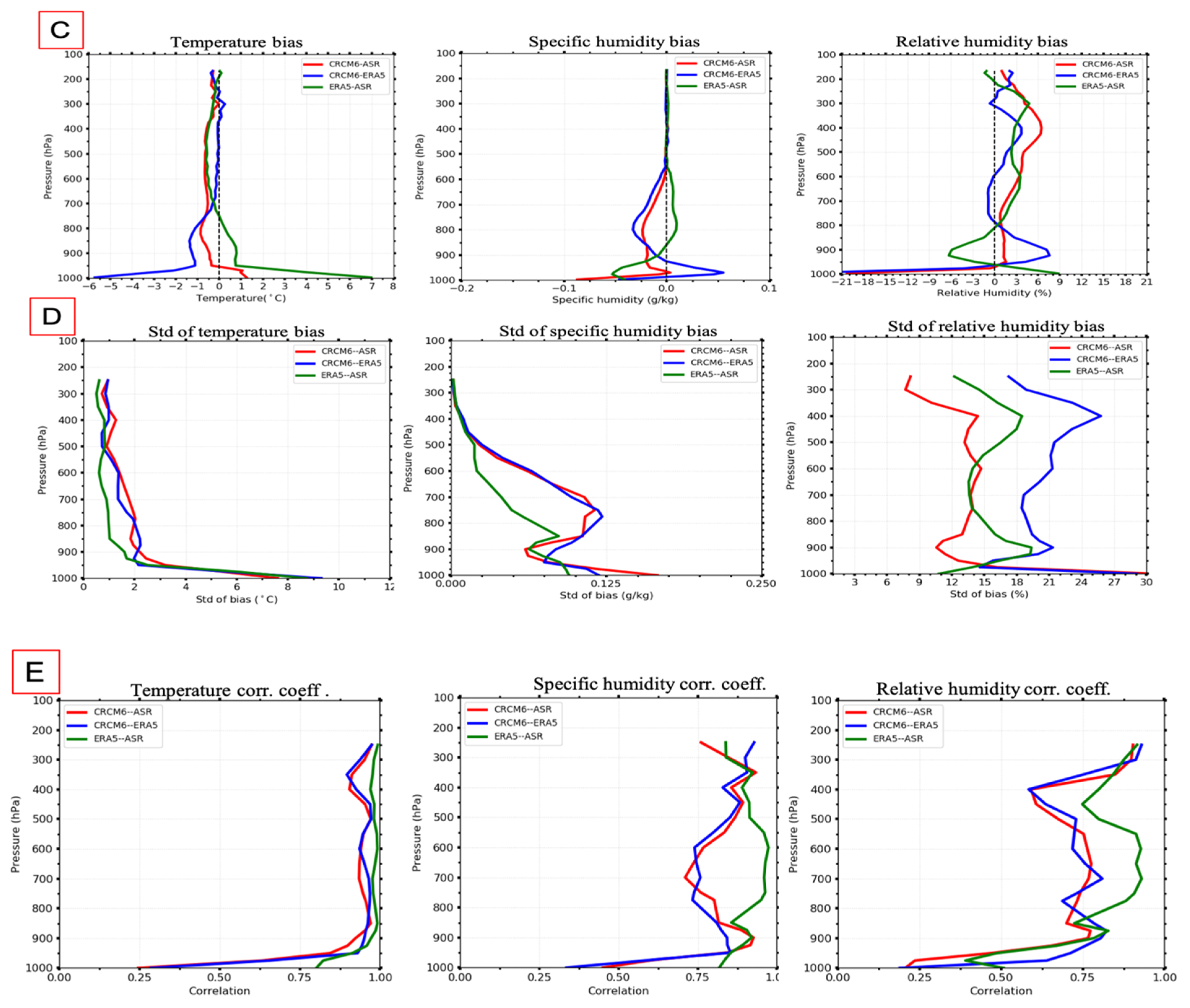
5.1. Meteorological Field Validation

Figure 2 shows a CRCM6 vs. ERA5 and ASR mean sea-level pressure (MSLP) (Figure 2A) and surface temperature (Figure 2B) across the 3 km mesh domain of Figure 1 for the reference month of January 2007. Biases are represented by white contour lines on the reanalysis maps. We note that, as a general statement, CRCM6 successfully reproduces the MSLP spatial patterns with bias amplitudes that are generally <1 hPa (except near the coast of Greenland which we avoided in our analyses). For the surface temperature, CRCM6 successfully reproduces the spatial patterns with bias amplitudes that are generally < 6 °C and negative for ERA5 and positive for ASR. We note a high density of biased contour lines near the coast of Greenland and North Atlantic which is due to uncertainties linked to surface processes such as orography and sea ice. Similar bias maps were generated for the specific humidity (SH) and relative humidity (RH) at 500 hPa (are not shown). The results were again of generally acceptable agreement: we leave the statistical interpretation of what that means to January 2007, pan-domain ensemble statistics of the analysis that follows.

Table 2. January 2007 mean and standard deviations (500 hPa and 900 hPa for the top and bottom tables respectively) across the 3 km mesh domain of Figure 1 for ASR and ERA5 and associated CRCM6 prediction bias for temperature, specific humidity, and relative humidity.

Models	ASR		ERA5		Bias (CRCM6-ASR)		Bias (CRCM6-ERA5)		Bias (ERA5-ASR)
Variables	mean	std	mean	std	mean	std	mean	std	mean	std
Temperature (°C)	−41.56	3.45	−41.94	3.63	−1.59	5.65	−0.39	0.82	−1.18	5.63
Specific humidity (g/Kg)	0.10	0.06	0.10	0.06	−0.03	0.09	−0.01	0.03	−0.02	0.09
Relative humidity (%)	47.75	15.99	33.50	17.01	0.06	23.44	−1.52	12.73	1.43	21.65
Models	ASR		ERA5		Bias (CRCM6-ASR)		Bias (CRCM6-ERA5)		Bias (ERA5-ASR)
Variables	mean	std	mean	std	mean	std	mean	std	mean	std
Temperature (°C)	−25.45	4.93	−21.76	4.76	−5.06	6.77	−0.78	1.96	0.76	6.66
Specific humidity (g/Kg)	0.56	0.33	0.56	0.29	−0.11	0.51	−0.05	0.18	−0.07	0.49
Relative humidity (%)	65.55	18.36	57.61	16.06	−1.67	25.73	−19.71	24.02	−0.19	21.65

shows January 2007, pan-domain, means and standard deviations for (i) the ASR and (ii) ERA5 reanalyses, the associated CRCM6 reanalysis biases relative to (iii) the ASR and (iv) ERA5 reanalysis as well as (v) the ERA5 biases relative to ASR for the temperature, the SH and RH across the CRCM6 domain of Figure 1 (500 and 900 hPa for the upper and lower tables respectively). Such a comparison enables a better appreciation of how the reanalysis-dependent variability of the key cloud-environment parameters might influence cloud simulation performance. The CRCM6-ERA5 mean and std (standard deviation) bias amplitudes are (except the mean RH bias) generally of smaller amplitude than the CRCM6-ASR bias: this is very likely since the former was used to drive the CRCM6 dynamics. The CRCM6-ERA5 temperature and SH std bias amplitudes at both 500 and 900 hPa are moderately smaller compared to their natural (std) variation (<41% and <64%) and significantly smaller than their natural mean (5% and 33%). In addition, the CRCM6-ERA5 temperature and SH bias std amplitudes were always less than their CRCM6-ASR and ERA5-ASR std analogs while their bias mean amplitudes were always less than their bias std amplitudes. The RH std bias amplitudes (relative to their natural std variation and natural mean) were notably larger (>149% and 42% respectively). In general, the large (relative) RH bias amplitudes are not unexpected given the known large uncertainties in modeled simulations of RH [28].

Figure 3 shows the 900 hPa (A) and 500 hPa (B) CRCM6, ERA5, and ASR (January 2007) time series of temperature, SH and RH (left-hand panels) as well as the CRCM6-ASR, CRCM6-ERA5, and ERA5-ASR biases (right-hand panels) at the “M” reference point of Figure 1. These temporal series can lend a degree of insight into what drives the statistics of Table 2 (despite the clear limitation in comparing parameter averages over the CRCM6 domain with the values at the single ‘’M’’ grid cell). We note that the typical variation of the temperature field with passing storms (increasing before storms and decreasing after, e.g., 25–26 January) is likely the greatest driver of the large temperature and SH std values of Table 2. The same type of general remarks made for the Table 2 CRCM6-ERA5 bias amplitudes apply to the day-to-day variations seen in Figure 3: in particular, one can visually observe the temperature and SH bias amplitudes that are substantial to moderately smaller than their natural variation while RH biases are notably larger. The time series biases in percentage can be found in the Supplementary Materials (Figure S5).

Figure 4 shows comparisons of (point “M”) CRCM6, ERA5 and ASR time-averaged vertical profiles of temperature, SH and RH (left to right panels) along with their bias means, bias stds, and (Pearson) correlation coefficients (top to bottom panel-rows respectively) for January 2007. The bias mean and bias std temperature amplitudes are <2 °C) except in the region of the inversion layer (<900 hPa) where they can be up to ~9 °C (Figure 4C,D, left-hand panels). The difficulty all models appear to have in capturing the polar winter inversion layer might be tied to the difficulties in simulating net heat fluxes in the very stable (thermally deep) polar winter boundary layer (see [63] for a discussion of modeling challenges). The mean SH profile (Figure 4A middle panel) is similar in form to that of temperature (Figure 4A left-hand panel) The amplitudes of the dominating bias std values are fairly large in the inversion layer as well as above the inversion layer (<0.15 and 0.125 g kg⁻¹ respectively). The RH profile of Figure 4c exhibits a gradual decrease with height, from 70% to 80% near the surface to very low values (<10%) in the stratosphere. The std bias profile spikes to large inversion layer amplitudes of >30% amplitude at 1000 hPa and values as high as 24% above the inversion layer. Figure 4E left-hand to right-hand respectively show the correlation coefficient profiles between temperature, SH, and RH (larger values being typically associated with lower frequency variations at higher altitudes). Temperature shows relatively high correlations (>0.9) above the inversion layer (vs. >0.6 for the humidity parameters).

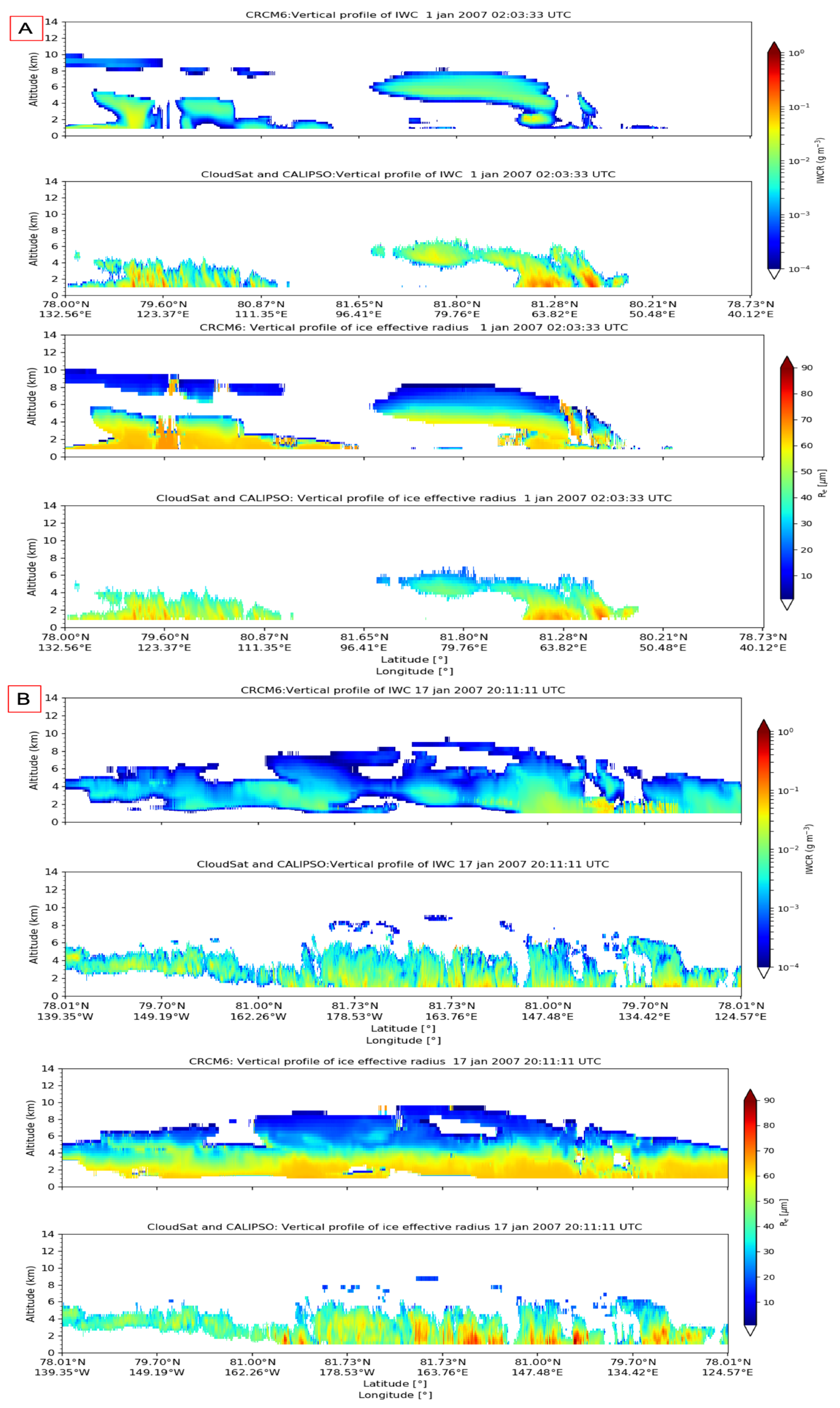
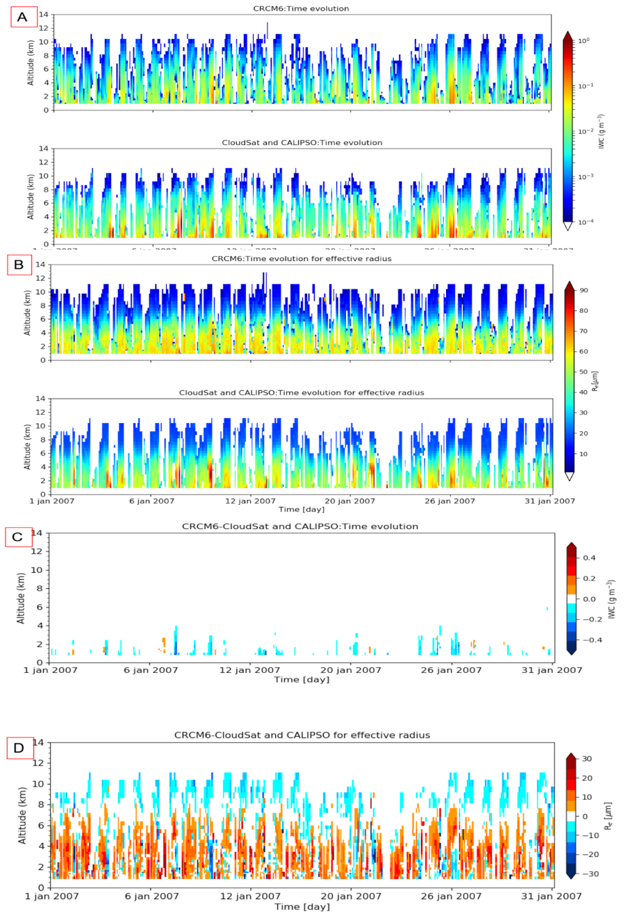
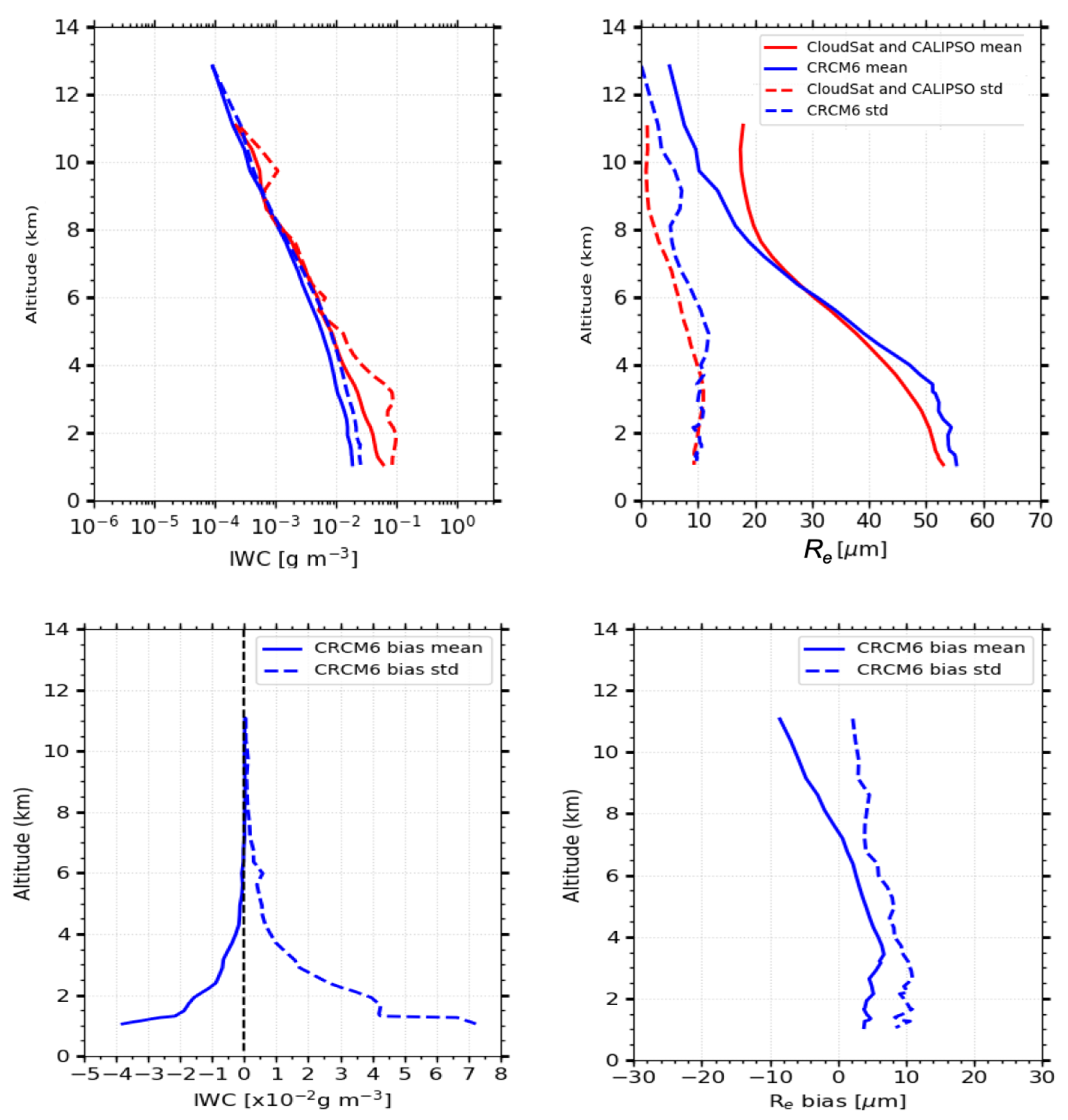
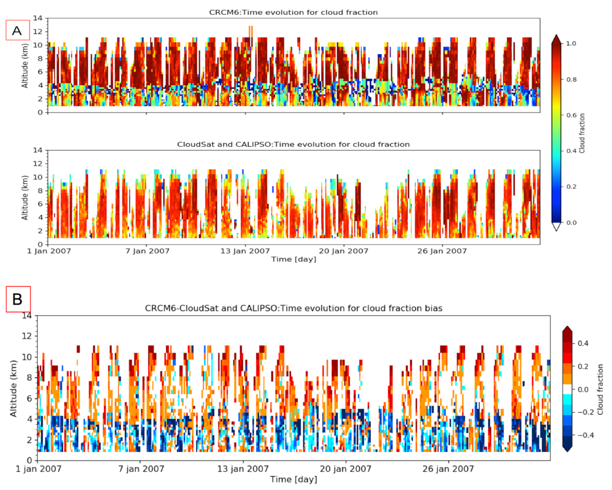
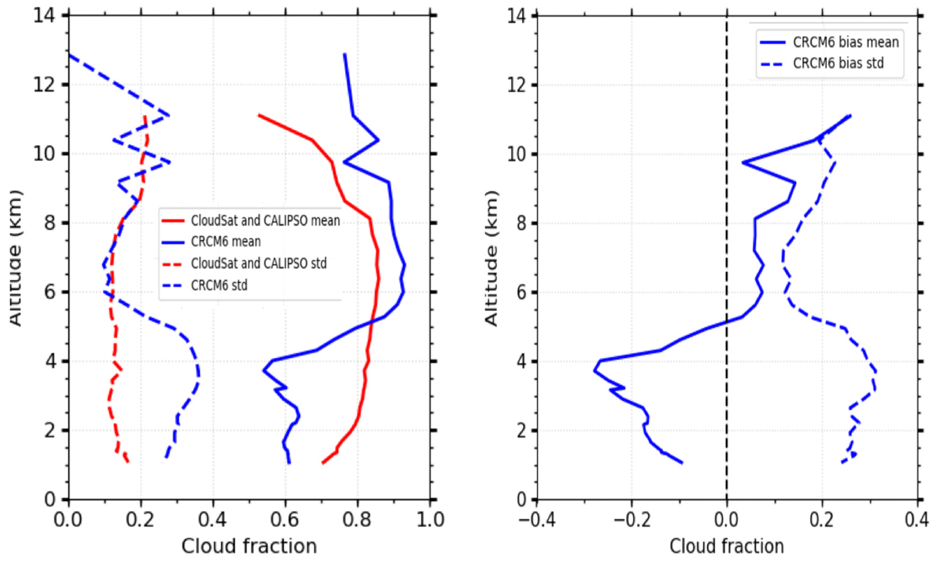
5.2. Optical Property Simulation of TICs

The analysis of CRCM6 skill in reproducing standard reanalysis parameters in the previous section was carried out to better understand CRCM6 performance in simulating ice water content (IWC) and effective radius (re) as well as associated heating rate profiles retrievals. Despite non-negligible bias mean and std differences in temperature and humidity, we expect cloud proprieties to still be relatively well constrained by the approximate level of accuracy that is attained (see, for example, the discussion in [28]). CRCM6 profile simulations of those TIC parameters were compared to CloudSat-CALIPSO 2C-ICE retrievals for every available orbit line during the January 2007 reference period (414 lines). To illustrate these event-level comparisons, we selected orbit lines that showed a considerable degree of IWC and re variation (1 and 17 January orbit lines of Figure 5A,B). This comparison enabled an appreciation of the event-level details of the cloud dynamics that, in turn, often gave insight into the scaled-up dynamics of time-averaged vertical profiles.

1 January (Figure 5A) was influenced by two cloud systems: mid to lower tropospheric clouds around 79.60° N and an upper troposphere to low troposphere system around 81.3° N while 17 January (Figure 5B) appeared to be subject to a generally cloudy system that stretched across the orbit line. The IWC simulations for both days show the same general cloud structure as the satellite observations of (stronger) IWC amplitude (satellite IWC > 10⁻² g m⁻³) while capturing higher altitude (small-re) cloud structures (the dark blue, re > 10 μm regions in the CRCM6 re profiles of Figure 5A,B) which were not detected by CloudSat (but were detected by CALIOP). This simulated, small-re result is coherent with Grenier et al. [27] who observed that sub−15 μm TIC particles could not be detected by CloudSat). On the other hand, the 1 and 17 January (reddish colored) fall lines that are readily observable in the satellite-derived re profiles (and that are likely indicative of large-re precipitating clouds) are, at best, only reproduced as “smeared” low frequency re increases by CRCM6 (a result attributable to the relatively low vertical and horizontal resolutions of CRCM6).

A temporal comparison of 2C-ICE and CRCM6-simulated vertical profiles of IWC and re during the reference month of January 2007 is shown in Figure 6A,B while Figure 6C shows the associated CRCM6 estimation biases relative to the 2C-ICE retrievals (orbit-dependent vertical profiles, see the figure caption). The simulated vertical and horizontal IWC structures are generally similar to the 2C-ICE profiles with a tendency for CRCM6 simulations to be of moderately lower amplitude (generally negative biases in Figure 6C). The largest negative biases can often be associated with the presence of a storm: we believe, for example, that this is the case for the dark blue negative bias on 8 January (when the low temperature profiles of Figure 3 suggested the presence of a winter storm). In such conditions, models tend to lag behind high-frequency physical processes such as small-scale turbulence.

The re profiles (Figure 6B) show simulated and observed vertical and horizontal structures that resemble the IWC profiles in terms of the amplitude patterns (notably in the case of the 2C-ICE profiles). At low altitudes (<~6 km) the CRCM6 simulations tend to be of lower amplitude than the occasional (reddish) spikes seen in the re profile while generally being of higher amplitude during times that exclude the spikes. This is borne out by the biases of Figure 6D (showing a generally positive bias pattern in the presence of sharp bluish spikes). At higher altitudes, those biases turn negative.

Figure 7 shows the (January 2007) CRCM6 simulated (blue) and 2C-ICE retrieved (red) IWC and re vertical profile means (solid lines) and stds (dashed lines) as well as the CRCM6-estimation biases for the orbit-dependent domain described in the legend of Figure 6. The mean IWC profiles differ little between ~6 and 9 km altitudes: below ~6 km, the CRCM6 profiles are weaker than their 2C-ICE counterparts (with attendant negative bias means). The re values from CRCM6 are stronger and weaker (respectively below and above ~6 km) with maximum bias mean deviations of ~6 and −10 µm, respectively. Finally, the CRCM6 IWC profile places clouds higher in the atmosphere compared to 2C-ICE (up to ~11 km): an observation that is not incoherent with the Figure 5 illustrations.

Figure 8A shows a time series comparison of CRCM6-simulated and 2B-GEOPROF-LIDAR profiles of cloud fraction, while Figure 8B shows the associated biases. The vertical and horizontal cloud fraction patterns are similar and generally show a level of moderate agreement in amplitude. The CRCM6 cloud fraction biases are generally positive for altitudes above 4–5 km. This is likely due to the model attributing a cloud fraction of unity if there is any cloud in a given model cell. This extreme attribution results when the model employs explicit (coarse, cell-level resolution) cloud fraction processing as opposed to implicit (microphysical resolution) processing. The negative (<−0.2) cloud fraction biases below 5–4 km altitude are likely the result of more realistic implicit processing.

Figure 9 (left hand panel) shows the mean vertical profiles (solid lines) and the standard deviations (dashed lines) of the CRCM6 (blue) and 2B-GEOPROF-LIDAR (red) cloud fraction. The mean profiles near the surface (<4–5 km) are ~0.6 for CRCM6 and ~0.8 for 2B-GEOPROF-LIDAR. The CRCM6 profile increases in amplitude to ~0.9 while the 2B-GEOPROF-LIDAR remains roughly constant up to 8 km of altitude. This results in a positive bias mean at altitudes > 5 km and a negative bias as ~−0.2 for altitudes < 5 km (Figure 9, right-hand panel). The sub-5km negative bias is arguably consistent with the positive re bias if the model crystals precipitate out faster than the real precipitation rate. The CRCM6 and 2B-GEOPROF-LIDAR std profiles are small and very similar above ~6 km. The std values below 4 km for CRCM6 are relatively large. The CRCM6 bias std of ~0.6 (increasing to ~0.9) in the right-hand panel of Figure 9 underscores the large cloud fraction variability for low-level (and high-level) CRCM6 clouds.

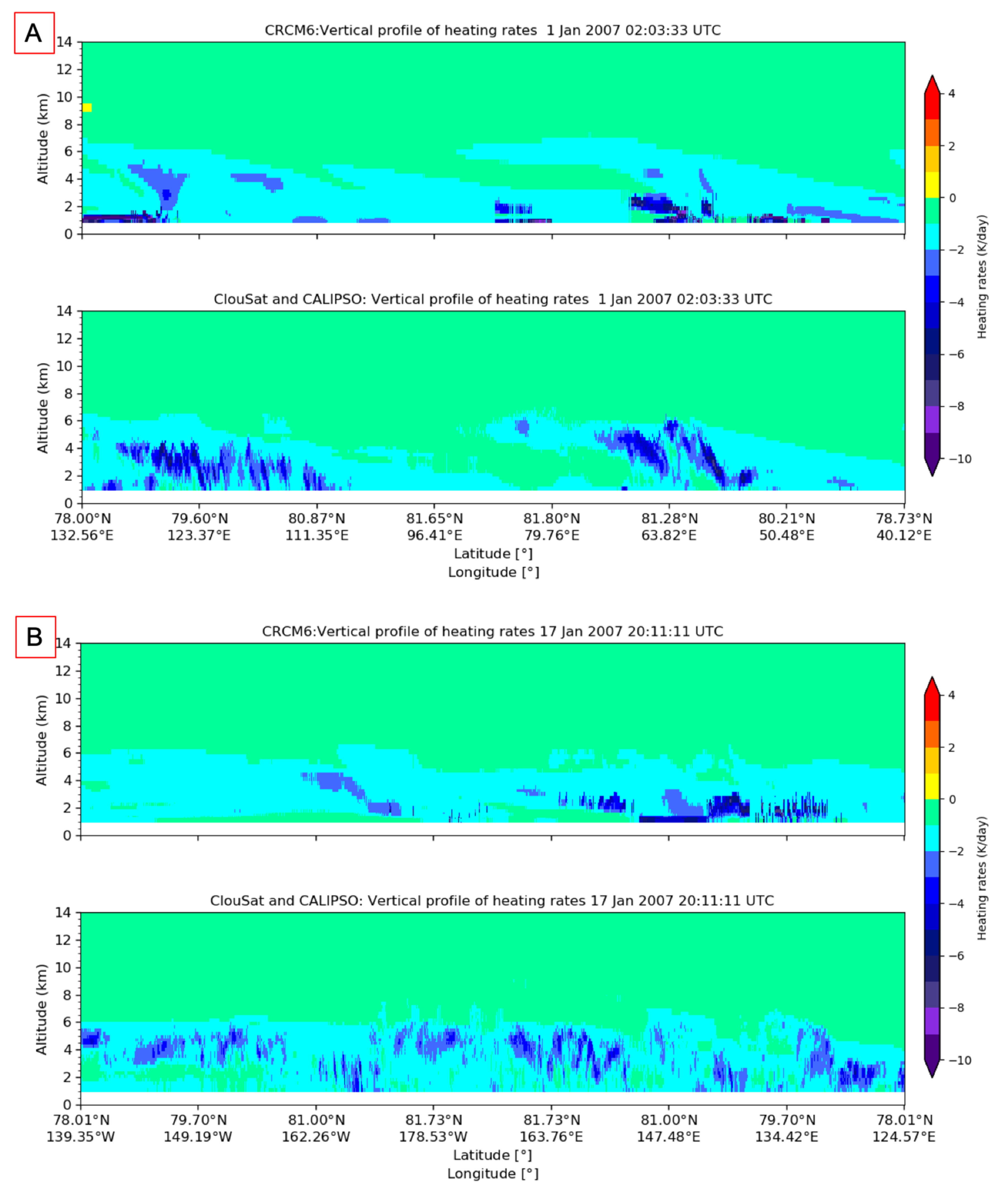
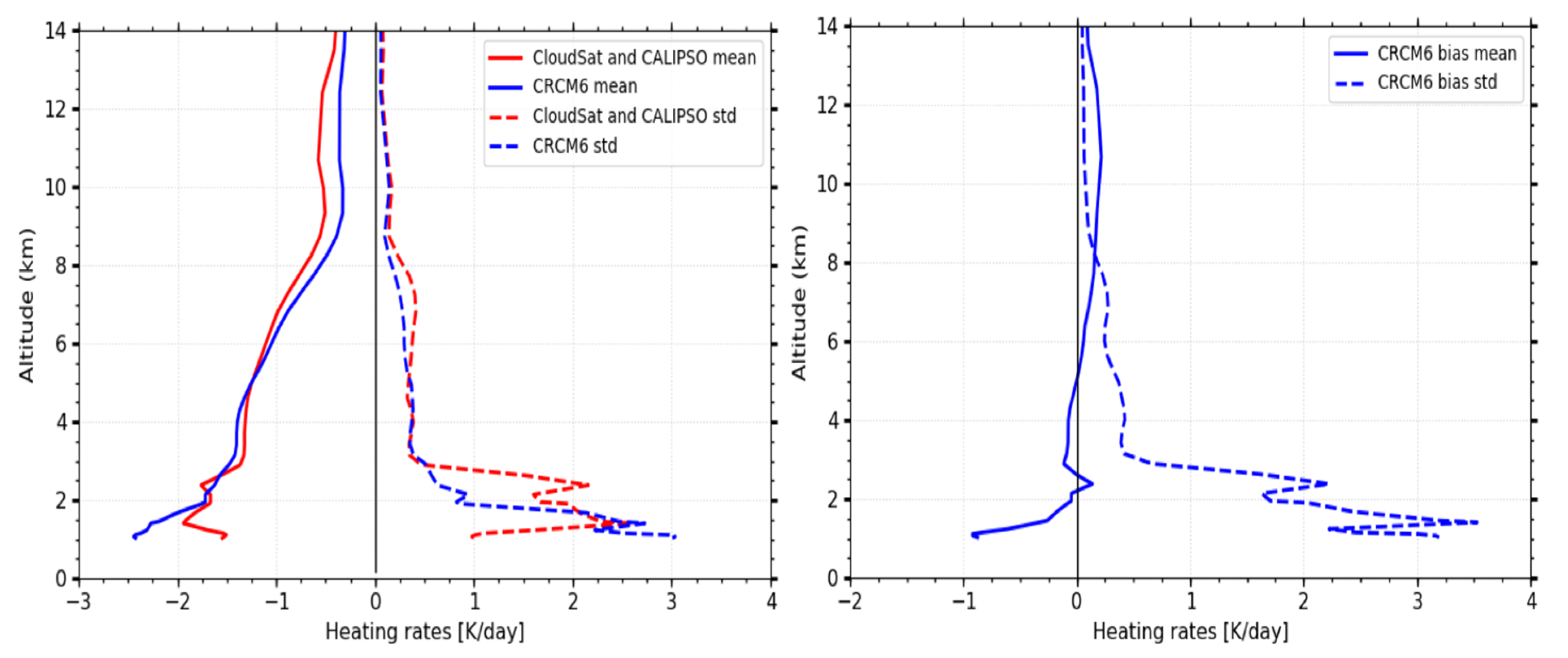
5.3. Cloud Heating Rates

The 1 and 17 January 2007 (Figure 7) CRCM6 and satellite-retrieved vertical profiles of ice properties were transformed into vertical profiles of (largely negative or cooling) diabatic heating rates (Figure 10A,B). The Jan. 1 CRCM6 heating rate profiles indicate vertical and horizontal structures that are similar to their IWC (and re) profiles while the similarities with 2B-FLXHR-LIDAR profiles are largely in terms of broad (low spatial frequency) variations; these include the general position of the two ice-cloud systems mentioned in the discussion of Figure 5, stronger amplitude cooling in the lower parts of these systems and a general cyan-colored system that only corresponds to certain broad patches of the Figure 5 cloud structure. CALIOP profiles of attenuated backscatter coefficient (see the 1 January 2007 example in Supplementary Materials Figure S1–S4) and depolarization ratio suggest that the high spatial variability of water and ice cloud mixing (and possibly, the higher concentrations of submicron aerosols) could complicate the 2B-FLXHR-LIDAR transformation to heating rates (and thus the level of agreement with CRCM6 heating rate profiles). Very similar comments can be made for the comparison between the CRCM6 17 January heating rate profile and its associated CRCM6 IWC/re profile as well as the correspondence between the former and the 2B-FLXHR-LIDAR heating rate profile. In general, CRCM6 and 2B-FLXHR-LIDAR show comparable, low-frequency diabatic heating rates ranging from 0 °K day⁻¹ to −8 °K day⁻¹ for our two illustrative events.

Figure 11A shows the time series of CRCM6-simulated versus 2B-FLXHR-LIDAR diabatic-heating rate profiles while Figure 11B shows the associated biases. The broad (low frequency), vertical, and horizontal heating rate patterns are (in keeping with our comment on the 1 and 17 January illustrations) generally in good agreement, with generally negative heating rate biases > −3 °K day⁻¹ interspersed by high-frequency positive bias “spikes” < 2 °K day⁻¹ when CRCM6 tends to overestimate cooling rates (corresponding to the warm-colored bias spikes of Figure 11B). Some notable examples are on 2, 7, 11, and 14 January: these likely correspond to storm variability episodes or time lags in the synoptic system (reanalysis) trajectory (time lags between the nominal reanalysis times and CALIOP/Cloudsat times).

Figure (left hand panel) shows the mean vertical profiles (solid lines) and the standard deviations (dashed lines) of the CRCM6 (blue) and 2B-FLXHR-LIDAR (red) heating rates (derived from the ensemble of individual orbit-line variations of Figure 11b). The mean vertical profiles are both ~−2 °K day−1 near the surface: they then decrease in amplitude to values ~−0.3 °K day⁻¹ at the highest altitude. Their similarity results in a small bias mean except very near the surface (amplitude < 0.25 °K day⁻¹ for altitudes > 2 km according to Figure 12 right-hand panel). The CRCM6 and 2B-FLXHR-LIDAR std profiles are small above ~3 km: this, we would argue, is at least partly attributable to weak polar-night temperature variability. The relatively large bias std values below 3 km are not unrelated to the large CRCM6 and 2B-FLXHR-LIDAR std variations in the same altitude region.

6. Discussion and Conclusions

We assessed the skill of the developmental Canadian Regional Climate Model version 6 (CRCM6) in simulating polar-night TICs and their effects on radiative cooling rates. This evaluation was carried out on a series of vertical-profile CALIOP/CloudSat satellite observations acquired during January of the 2007 International Polar Year (IPY). Our immediate goal (in preparation for a broader climatological-scale statistical analysis) was to analyze event-level TIC properties and radiative responses along with individual orbit-line vertical profiles as well as averages over the entire month: this enabled an initial assessment of CRCM6 cloud microphysics simulation performance at the process scale before reverting to statistical aggregation. A secondary motivation for this work was related to the NASA Aerosol-Cloud, Convection, and Precipitation (A-CCP) mission: we seek to employ the IPY data as a testbed for end-to-end, A-CCP-related instrument simulations at high latitudes. The IPY CALIOP/CloudSat profiles were supported by ground-based retrievals, campaign data, and numerous auxiliary atmospheric databases (such as ERA5 and ASR reanalyses).

We tested the ability of CRCM6 to reproduce observed meteorological systems on a synoptic scale (~1000 km) and to adequately simulate high-resolution clouds and other physical processes. We verified that the spatial patterns of pressure, temperature, and humidity (averaged over the reference month of January 2007) remained close to the ERA5 and ASR reanalyses (while CRCM6 generates its fine-scale structure and local weather conditions, it must nonetheless upscale to the lower resolution reanalysis data). Admittedly, these reanalysis references also retain a portion of their model biases on top of all available observations that are included in the database. The comparisons with the two reanalysis references were carried out to better appreciate meteorological parameter uncertainty within the context of two independently generated reanalysis data sets. We presented the specific illustration of how CRCM6 adequately simulated the spatial MSLP and surface temperature patterns across the CRCM6 domain of Figure 1 (bias contour amplitudes < 1 hPa, <6 °C respectively for MSLP and surface temperature with larger amplitudes in the vicinity of the high elevations of Greenland).

We quantified, in an average sense, the affirmations of CRCM6 spatial pattern performance by investigating the pan-domain (500 and 900 hPa) CRCM6 bias means and stds of temperature, SH, and RH relative to the ASR and ERA5 reanalyses for the reference month of January 2007. CRCM6 generally performed better relative to ERA5 (except in the case of RH) because ERA5 had been employed to nudge the CRCM6 domain. In general, the CRCM6–ERA5 temperature and SH std bias amplitudes at both 500 and 900 hPa are moderately smaller compared to their natural (std) variation (<41% and <64%) and significantly smaller than their natural mean (5% and 33%). The CRCM6-ERA5 temperature and SH bias std amplitudes were less than their CRCM6-ASR and ERA5-ASR std analogs while their bias mean amplitudes were less than their bias std amplitudes. The RH std bias amplitudes relative to their natural std variation and mean were notably larger (>149% and 42%).

The time series for the same three parameters and the same reference month at a single point (point “M” of Figure 1) showed a degree of coherency with the monthly averaged, pan-domain statistics. We noted that the typical variation of the temperature field with passing storms (increasing before storms and decreasing after) is likely the greatest driver of the large temperature and SH variations. It was suggested that the generally larger inversion layer bias mean and bias std values for (point ‘’M’’) vertical profiles of the 3 key meteorological parameters over the January 2007 reference month were due to modeling difficulties in simulating net heat fluxes in the thermally-deep, polar-winter boundary layer. Vertical profiles of the correlation coefficient between CRCM6, ERA5, and ASR reanalyses showed a rapid increase in correlation above the inversion layer.

Having analyzed the general level of agreement in terms of the key meteorological/thermodynamic variables, we analyzed the CRCM6 simulations of ice cloud properties. Comparisons of selected events on 1 and 17 January showed that the (relatively low spatial resolution) CRCM6 simulations captured the low-frequency IWC and re features of the 2C-ICE (satellite-derived) cloud banks for satellite IWC values > 10⁻² g m⁻³. The fact that CRCM6 captured high altitude, small re features was attributed to the fact that CloudSat becomes insensitive to small ice particles (re < 15 µm). In terms of the January 2007 (reference month) time series of (orbit-line averaged) IWC, re and cloud fraction profiles, CRCM6 appeared to capture the essential IWC features of the satellite profiles while generally tending to underestimate (bias negatively) its predictions. The most negative biases seemed to be induced around the time of winter storms. A time-series comparison for the complete reference month showed that CRCM6 generally tended to capture the IWC variations while moderately underestimating their value. A similar comparison for the re profiles showed CRCM6 overestimating re below ~6 km (with occasional spikes of underestimation) and underestimating above ~6 km (likely attributable to the CloudSat lower sensitivity limit of 15 µm). A comparison of cloud fraction profiles showed a negative CRCM6 cloud fraction bias near the surface: an associated positive re bias suggested that the model precipitates out faster than the observations. The cloud fraction std bias of 0.6 and 0.9 at lower and higher altitudes indicated a fairly large CRCM6 cloud fraction variability.

In general, the heating rate profiles were largely negative (cooling rates). The illustrative CRCM6 (1 January and 17 January) heating rate profiles showed, not surprisingly, a level of spatial coherence with their associated CRCM6 IWC and re profiles, while showing a degree of low-frequency coherency with the 2B-FLXHR-LIDAR heating rate profiles. A time series of CRCM6 vs. 2B-FLXHR-LIDAR comparisons across the 2007 reference month showed that the broad, vertical, and horizontal heating rate patterns were generally in good agreement (negative heating rate biases > −3 °K day⁻¹ accompanied by high-frequency positive bias “spikes” < 2 °K day⁻¹). CRCM6 vertical-profile heating rate comparisons with 2B-FLXHR-LIDAR over the total January 2007 reference month showed strong similarities except near the surface (small bias mean amplitude < 0.25 °K day⁻¹ for altitudes > 2 km). These similarities were, at least partly, ascribed to weak polar-night temperature variability.

Our results largely support the use of the CRCM6 model for studying the physical processes and energetics associated with cloud types in the polar atmosphere. The new CRCM6 version successfully simulated low spatial frequency polar winter cloud properties and their associated impact on heating rates. The CRCM6 simulations captured the presence of small, UTLS (TIC1) ice crystals that the 2C-ICE product failed to detect. This was ascribed to the CloudSat insensitivity to TICs of re < 15 µm. High-Arctic, polar-night, air-mass cooling is largely the result of IR radiation dynamics: ice cloud contributions may very likely dominate these dynamics and thus the Arctic atmosphere radiation balance. It is therefore critical to ensure model reliability in representing cloud proprieties and their effects on atmosphere energetics. The availability of remotely sensed ice-cloud data sets, as well as high-resolution simulations, enables comparisons between satellite observations and models. The observed CRCM6 simulation performance with regard to ice-cloud properties and ice-cloud heating rates enables an improved understanding of the dynamics of the high-Arctic energy cycle and its potential contributions to storm development.

References

1. Hassol, S.J. Impacts of a Warming Arctic-Arctic Climate Impact Assessment; Cambridge University Press: Cambridge, UK; New York, NY, USA, 2004. [Google Scholar]
2. Alexander, L.V. Global observed long-term changes in temperature and precipitation extremes: A review of progress and limitations in IPCC assessments and beyond. Weather Clim. Extrem. 2016, 11, 4–16. [Google Scholar] [CrossRef] [Green Version]
3. Comiso, J.C. Warming trends in the Arctic from clear sky satellite observations. J. Clim. 2003, 16, 3498–3510. [Google Scholar] [CrossRef] [Green Version]
4. Comiso, J.C. Arctic warming signals from satellite observations. Weather 2006, 61, 70–76. [Google Scholar] [CrossRef] [Green Version]
5. Liu, Y.; Key, J.R.; Wang, X. The influence of changes in cloud cover on recent surface temperature trends in the Arctic. J. Clim. 2008, 21, 705–715. [Google Scholar] [CrossRef]
6. Liu, Y.; Key, J.R.; Wang, X. Influence of changes in sea ice concentration and cloud cover on recent Arctic surface temperature trends. Geophys. Res. Lett. 2009, 36, 705–715. [Google Scholar] [CrossRef] [Green Version]
7. Keita, S.A.; Girard, E. Importance of Chemical Composition of Ice Nuclei on the Formation of Arctic Ice Clouds. Pure Appl. Geophys. 2016, 173, 3141–3163. [Google Scholar] [CrossRef]
8. Intrieri, J.M.; Shupe, M.D. Characteristics and radiative effects of diamond dust over the western Arctic Ocean region. J. Clim. 2004, 17, 2953–2960. [Google Scholar] [CrossRef]
9. Libois, Q.; Blanchet, J.P. Added value of far-infrared radiometry for remote sensing of ice clouds. J. Geophys. Res. Atmos. 2017, 122, 6541–6564. [Google Scholar] [CrossRef] [Green Version]
10. Curry, J.A.; Schramm, J.L.; Rossow, W.B.; Randall, D. Overview of Arctic cloud and radiation characteristics. J. Clim. 1996, 9, 1731–1764. [Google Scholar] [CrossRef] [Green Version]
11. Blanchet, J.-P.; Royer, A.; Châteauneuf, F.; Bouzid, Y.; Blanchard, Y.; Hamel, J.-F.; de Lafontaine, J.; Gauthier, P.; O’Neill, N.T.; Pancrati, O. TICFIRE: A far infrared payload to monitor the evolution of thin ice clouds. In Proceedings of the Sensors, Systems, and Next-Generation Satellites XV, Prague, Czech Republic, 19–22 September 2011; p. 81761K. [Google Scholar]
12. Chen, T.; Rossow, W.B.; Zhang, Y. Radiative effects of cloud-type variations. J. Clim. 2000, 13, 264–286. [Google Scholar] [CrossRef]
13. Kahl, J.D. Characteristics of the low-level temperature inversion along the Alaskan Arctic coast. Int. J. Climatol. 1990, 10, 537–548. [Google Scholar] [CrossRef]
14. Kahl, J.D.; Serreze, M.C.; Schnell, R.C. Tropospheric low-level temperature inversions in the Canadian Arctic. Atmos.-Ocean. 1992, 30, 511–529. [Google Scholar] [CrossRef]
15. Persson, P.; Uttal, T.; Intrieri, J.; Fairall, C.; Andreas, E.; Guest, P. Observations of large thermal transitions during the Arctic night from a suite of sensors at SHEBA. In Proceedings of the Preprints, Fifth Conference on Polar Meteorology and Oceanography, Virtual, 1–4 June 2021; pp. 10–15. [Google Scholar]
16. Persson, P.O.G.; Fairall, C.W.; Andreas, E.L.; Guest, P.S.; Perovich, D.K. Measurements near the Atmospheric Surface Flux Group tower at SHEBA: Near-surface conditions and surface energy budget. J. Geophys. Res. Ocean. 2002, 107, SHE 21-1–SHE 21-35. [Google Scholar] [CrossRef] [Green Version]
17. L’Ecuyer, T.S.; Wood, N.B.; Haladay, T.; Stephens, G.L.; Stackhouse, P.W., Jr. Impact of clouds on atmospheric heating based on the R04 CloudSat fluxes and heating rates data set. J. Geophys. Res. Atmos. 2008, 113, D00A15. [Google Scholar] [CrossRef] [Green Version]
18. Oreopoulos, L.; Cho, N.; Lee, D.; Kato, S.; Huffman, G.J. An examination of the nature of global MODIS cloud regimes. J. Geophys. Res. Atmos. 2014, 119, 8362–8383. [Google Scholar] [CrossRef] [Green Version]
19. Girard, E.; Blanchet, J.-P.; Dubois, Y. Effects of arctic sulphuric acid aerosols on wintertime low-level atmospheric ice crystals, humidity and temperature at Alert, Nunavut. Atmos. Res. 2005, 73, 131–148. [Google Scholar] [CrossRef]
20. Girard, E.; Dueymes, G.; Du, P.; Bertram, A.K. Assessment of the effects of acid-coated ice nuclei on the Arctic cloud microstructure, atmospheric dehydration, radiation and temperature during winter. Int. J. Climatol. 2013, 33, 599–614. [Google Scholar] [CrossRef]
21. Dufresne, J.-L.; Bony, S. An assessment of the primary sources of spread of global warming estimates from coupled atmosphere–ocean models. J. Clim. 2008, 21, 5135–5144. [Google Scholar] [CrossRef] [Green Version]
22. Shupe, M.D.; Walden, V.P.; Eloranta, E.; Uttal, T.; Campbell, J.R.; Starkweather, S.M.; Shiobara, M. Clouds at Arctic atmospheric observatories. Part I: Occurrence and macrophysical properties. J. Appl. Meteorol. Climatol. 2011, 50, 626–644. [Google Scholar] [CrossRef] [Green Version]
23. Uttal, T.; Curry, J.A.; McPhee, M.G.; Perovich, D.K.; Moritz, R.E.; Maslanik, J.A.; Guest, P.S.; Stern, H.L.; Moore, J.A.; Turenne, R. Surface heat budget of the Arctic Ocean. Bull. Am. Meteorol. Soc. 2002, 83, 255–276. [Google Scholar] [CrossRef] [Green Version]
24. Shupe, M.D. Clouds at Arctic atmospheric observatories. Part II: Thermodynamic phase characteristics. J. Appl. Meteorol. Climatol. 2011, 50, 645–661. [Google Scholar] [CrossRef]
25. Nikiéma, O.; Laprise, R. An approximate energy cycle for inter-member variability in ensemble simulations of a regional climate model. Clim. Dyn. 2013, 41, 831–852. [Google Scholar] [CrossRef] [Green Version]
26. Blanchet, J.-P.; Girard, E. Arctic ‘greenhouse effect’. Nature 1994, 371, 383. [Google Scholar] [CrossRef]
27. Grenier, P.; Blanchet, J.P.; Muñoz-Alpizar, R. Study of polar thin ice clouds and aerosols seen by CloudSat and CALIPSO during midwinter. J. Geophys. Res. Atmos. 2009, 114, D09201. [Google Scholar] [CrossRef] [Green Version]
28. Jouan, C.; Girard, E.; Pelon, J.; Gultepe, I.; Delanoë, J.; Blanchet, J.P. Characterization of Arctic ice cloud properties observed during ISDAC. J. Geophys. Res. Atmos. 2012, 117, D23. [Google Scholar] [CrossRef] [Green Version]
29. Keita, S.A.; Girard, E.; Raut, J.-C.; Leriche, M.; Blanchet, J.-P.; Pelon, J.; Onishi, T.; Cirisan, A. A new parameterization of ice heterogeneous nucleation coupled to aerosol chemistry in WRF-Chem model version 3.5. 1: Evaluation through ISDAC measurements. Geosci. Model Dev. 2020, 13, 5737–5755. [Google Scholar] [CrossRef]
30. Keita, S.A.; Girard, E.; Raut, J.-C.; Pelon, J.; Blanchet, J.-P.; Lemoine, O.; Onishi, T. Simulating Arctic Ice Clouds during Spring Using an Advanced Ice Cloud Microphysics in the WRF Model. Atmosphere 2019, 10, 433. [Google Scholar] [CrossRef] [Green Version]
31. Grenier, P.; Blanchet, J.P. Investigation of the sulphate-induced freezing inhibition effect from CloudSat and CALIPSO measurements. J. Geophys. Res. Atmos. 2010, 115, D22. [Google Scholar] [CrossRef] [Green Version]
32. Cirisan, A.; Girard, E.; Blanchet, J.-P.; Keita, S.A.; Gong, W.; Irish, V.; Bertram, A.K. CNT Parameterization Based on the Observed INP Concentration during Arctic Summer Campaigns in a Marine Environment. Atmosphere 2020, 11, 916. [Google Scholar] [CrossRef]
33. Jouan, C.; Pelon, J.; Girard, E.; Ancellet, G.; Blanchet, J.-P.; Delanoë, J. On the relationship between Arctic ice clouds and polluted air masses over the North Slope of Alaska in April. Atmos. Chem. Phys. 2014, 14, 1205–1224. [Google Scholar] [CrossRef] [Green Version]
34. Morrison, H.; Milbrandt, J.A. Parameterization of cloud microphysics based on the prediction of bulk ice particle properties. Part I: Scheme description and idealized tests. J. Atmos. Sci. 2015, 72, 287–311. [Google Scholar] [CrossRef]
35. Milbrandt, J.; Morrison, H. Parameterization of cloud microphysics based on the prediction of bulk ice particle properties. Part III: Introduction of multiple free categories. J. Atmos. Sci. 2016, 73, 975–995. [Google Scholar] [CrossRef]
36. Milbrandt, J.A.; Bélair, S.; Faucher, M.; Vallée, M.; Carrera, M.L.; Glazer, A. The Pan-Canadian high resolution (2.5 km) deterministic prediction system. Weather Forecast. 2016, 31, 1791–1816. [Google Scholar] [CrossRef]
37. Yang, J.; Jones, K.F.; Yu, W.; Morris, R. Simulation of in-cloud icing events on Mount Washington with the GEM-LAM. J. Geophys. Res. Atmos. 2012, 117, D17. [Google Scholar] [CrossRef] [Green Version]
38. Côté, J.; Gravel, S.; Méthot, A.; Patoine, A.; Roch, M.; Staniforth, A. The operational CMC–MRB global environmental multiscale (GEM) model. Part I: Design considerations and formulation. Mon. Weather Rev. 1998, 126, 1373–1395. [Google Scholar] [CrossRef]
39. Girard, C.; Plante, A.; Desgagné, M.; McTaggart-Cowan, R.; Côté, J.; Charron, M.; Gravel, S.; Lee, V.; Patoine, A.; Qaddouri, A. Staggered vertical discretization of the Canadian Environmental Multiscale (GEM) model using a coordinate of the log-hydrostatic-pressure type. Mon. Weather Rev. 2014, 142, 1183–1196. [Google Scholar] [CrossRef]
40. Laprise, R. The Euler equations of motion with hydrostatic pressure as an independent variable. Mon. Weather Rev. 1992, 120, 197–207. [Google Scholar] [CrossRef]
41. Bélair, S.; Mailhot, J.; Girard, C.; Vaillancourt, P. Boundary layer and shallow cumulus clouds in a medium-range forecast of a large-scale weather system. Mon. Weather Rev. 2005, 133, 1938–1960. [Google Scholar] [CrossRef]
42. Bélair, S.; Mailhot, J.; Strapp, J.W.; MacPherson, J.I. An examination of local versus nonlocal aspects of a TKE-based boundary layer scheme in clear convective conditions. J. Appl. Meteor. 1999, 38, 1499–1518. [Google Scholar] [CrossRef]
43. Takhsha, M.; Nikiéma, O.; Lucas-Picher, P.; Laprise, R.; Hernández-Díaz, L.; Winger, K. Dynamical downscaling with the fifth-generation Canadian regional climate model (CRCM5) over the CORDEX Arctic domain: Effect of large-scale spectral nudging and of empirical correction of sea-surface temperature. Clim. Dyn. 2018, 51, 161–186. [Google Scholar] [CrossRef]
44. Li, J.; Barker, H. A radiation algorithm with correlated-k distribution. Part I: Local thermal equilibrium. J. Atmos. Sci. 2005, 62, 286–309. [Google Scholar] [CrossRef]
45. Kain, J.S.; Fritsch, J.M. A one-dimensional entraining/detraining plume model and its application in convective parameterization. J. Atmos. Sci. 1990, 47, 2784–2802. [Google Scholar] [CrossRef] [Green Version]
46. Kuo, E. Wave scattering and transmission at irregular surfaces. J. Acoust. Soc. Am. 1964, 36, 2135–2142. [Google Scholar] [CrossRef]
47. Sundqvist, H.; Berge, E.; Kristjansson, J. Condensation and cloud parameterization studies with a mesoscale numerical weather prediction model. Mon. Weather Rev. 1989, 117, 1641–1657. [Google Scholar] [CrossRef]
48. Verseghy, D. The Canadian Land Surface Scheme: Technical Documentation—Version 3.4. 2008. Available online: http://citeseerx.ist.psu.edu/viewdoc/download?doi=10.1.1.614.4315&rep=rep1&type=pdf (accessed on 17 November 2021).
49. Verseghy, D.L. The Canadian land surface scheme (CLASS): Its history and future. Atmos.-Ocean. 2000, 38, 1–13. [Google Scholar] [CrossRef]
50. Cholette, M.; Morrison, H.; Milbrandt, J.A.; Thériault, J.M. Parameterization of the bulk liquid fraction on mixed-phase particles in the predicted particle properties (P3) scheme: Description and idealized simulations. J. Atmos. Sci. 2019, 76, 561–582. [Google Scholar] [CrossRef]
51. Milbrandt, J.; Yau, M. A multimoment bulk microphysics parameterization. Part I: Analysis of the role of the spectral shape parameter. J. Atmos. Sci. 2005, 62, 3051–3064. [Google Scholar] [CrossRef] [Green Version]
52. Sankaré, H.; Thériault, J.M. On the relationship between the snowflake type aloft and the surface precipitation types at temperatures near 0 °C. Atmos. Res. 2016, 180, 287–296. [Google Scholar] [CrossRef]
53. Heymsfield, A.J.; Miloshevich, L.M. Parameterizations for the cross-sectional area and extinction of cirrus and stratiform ice cloud particles. J. Atmos. Sci. 2003, 60, 936–956. [Google Scholar] [CrossRef]
54. Morrison, H.; Grabowski, W.W. A novel approach for representing ice microphysics in models: Description and tests using a kinematic framework. J. Atmos. Sci. 2008, 65, 1528–1548. [Google Scholar] [CrossRef] [Green Version]
55. Hersbach, H.; Bell, B.; Berrisford, P.; Biavati, G.; Dee, D.; Horányi, A.; Nicolas, J.; Peubey, C.; Radu, R.; Rozum, I. The ERA5 Global Atmospheric Reanalysis at ECMWF as a comprehensive dataset for climate data homogenization, climate variability, trends and extremes. Geophys. Res. Abstr. 2019, 21, EGU2019-10826-1. [Google Scholar]
56. Bromwich, D.H.; Wilson, A.B.; Bai, L.S.; Moore, G.W.; Bauer, P. A comparison of the regional Arctic System Reanalysis and the global ERA-Interim Reanalysis for the Arctic. Q. J. R. Meteorol. Soc. 2016, 142, 644–658. [Google Scholar] [CrossRef] [Green Version]
57. Deng, M.; Mace, G.G.; Wang, Z.; Okamoto, H. Tropical Composition, Cloud and Climate Coupling Experiment validation for cirrus cloud profiling retrieval using CloudSat radar and CALIPSO lidar. J. Geophys. Res. Atmos. 2010, 115, D00J15. [Google Scholar] [CrossRef] [Green Version]
58. Henderson, D.S.; L’Ecuyer, T.; Stephens, G.; Partain, P.; Sekiguchi, M. A multisensor perspective on the radiative impacts of clouds and aerosols. J. Appl. Meteorol. Climatol. 2013, 52, 853–871. [Google Scholar] [CrossRef]
59. Deng, M.; Mace, G.G.; Wang, Z.; Lawson, R.P. Evaluation of several A-Train ice cloud retrieval products with in situ measurements collected during the SPARTICUS campaign. J. Appl. Meteorol. Climatol. 2013, 52, 1014–1030. [Google Scholar] [CrossRef] [Green Version]
60. Mace, G.G.; Zhang, Q. The CloudSat radar-lidar geometrical profile product (RL-GeoProf): Updates, improvements, and selected results. J. Geophys. Res. Atmos. 2014, 119, 9441–9462. [Google Scholar] [CrossRef]
61. Stephens, G.L.; Tsay, S.-C.; Stackhouse, P.W., Jr.; Flatau, P.J. The relevance of the microphysical and radiative properties of cirrus clouds to climate and climatic feedback. J. Atmos. Sci. 1990, 47, 1742–1754. [Google Scholar] [CrossRef]
62. Stephens, G.L.; Gabriel, P.M.; Partain, P.T. Parameterization of atmospheric radiative transfer. Part I: Validity of simple models. J. Atmos. Sci. 2001, 58, 3391–3409. [Google Scholar] [CrossRef]
63. Beare, R.J.; Macvean, M.K.; Holtslag, A.A.; Cuxart, J.; Esau, I.; Golaz, J.-C.; Jimenez, M.A.; Khairoutdinov, M.; Kosovic, B.; Lewellen, D. An intercomparison of large-eddy simulations of the stable boundary layer. Bound.-Layer Meteorol. 2006, 118, 247–272. [Google Scholar] [CrossRef] [Green Version]
Figure 1. Study domain: The black outer box is the 12 km mesh CRCM6 domain (340 × 340 grid points). The blue inner box is the 3 km mesh CRCM6 domain (700 × 700 grid points). The red-dashed box is the domain of comparisons between the CRCM6 and CloudSat-CALIPSO data (the region of Greenland was explicitly excluded to avoid the non-representative dynamics of its high-elevation terrain). The arrow labeled “(M)” indicates the specific grid point that was employed to analyze specific dynamics details of CRCM6 profiles (see Figures 3 and 4).
Atmosphere 13 00187 g001
Figure 2. (A) January 2007 MSLP (mean sea-level pressure) time averages and biases (white contours) of sea level pressure and (B) surface temperature time averages and biases across the 3 km mesh domain of Figure 1, left-hand panels CRCM6, in the middle ERA5 and CRCM6-ERA5 and right-hand panels ASR and CRCM6-ASR. Note that the white contours being smooth continuous curves is not the result of some post-processing enhancement of the contouring program: rather the stepped color key does not do justice to detailed MSLP spatial variation.
Atmosphere 13 00187 g002
Figure 3. January, 007 time series of temperature, specific humidity and relative humidity (left-hand panels), and biases (right-hand panels) at the “M” grid point of Figure 1. The individual points of the curves are daily averages. (A) 900 hPa and (B) 500 hPa. The legend in the top two panels shows the different reanalysis models.
Atmosphere 13 00187 g003
Figure 4. Vertical profiles of CRCM6, ASR, and ERA5 temperature, specific humidity, and relative humidity at the “(M)” gridpoint of Figure 1 for January 2007. (A,B): monthly averages and stds. (C,D) bias difference means and stds. (E) correlation coefficients.
Atmosphere 13 00187 g004aAtmosphere 13 00187 g004b
Figure 5. CRCM6-simulated and CloudSat-CALIPSO ICE-2C retrievals of IWC and re vertical profiles for (A) 1 January and (B) 17 January 2007.
Atmosphere 13 00187 g005
Figure 6. Time evolution of (CloudSat-Calipso) retrieved and CRCM6-simulated IWC (A) and re (B) vertical profiles for January 2007. Each thin (colored) vertical strip represents an orbit-line average for the 6 to 8 orbit lines that typically cross the CRCM6 domain of Figure 1 in a single day. The associated CRCM6-simulated vertical profile biases are shown in the lower two panels (C,D).
Atmosphere 13 00187 g006
Figure 7. Top panels: vertical profile averages (solid curves) and stds (dashed curves) of IWC (left-hand panels) and ice re (right-hand panels) from CRCM6 simulations (blue curves) and ICE-dust retrievals (red curves) over the reference month of January 2007. The bottom panel profiles show the mean and std of the CRCM6 biases relative to the ICE-dust retrievals.
Atmosphere 13 00187 g007
Figure 8. Time evolution of cloud fraction simulated by CRCM6 and retrieved from CloudSat-CALIPSO profiles (A) and bias (B).
Atmosphere 13 00187 g008
Figure 9. Vertical profiles of cloud fraction statistics: the solid and dashed curves in the left-hand panel represent, respectively, the average and standard deviation over the profiles of Figure 8A while the blue and red colors represent CRCM6 simulations and CloudSat-CALIPSO retrievals respectively. The right-hand panel shows the bias of the CRCM6 profiles relative to the Cloud-Sat-CALIPSO profiles: the solid-line and dashed-line profiles represent the bias mean and bias std respectively over the profiles of Figure 8B.
Atmosphere 13 00187 g009
Figure 10. Vertical profiles of CRCM6-simulated and CloudSat-CALIPSO retrieved radiation heating rates. (A) 1 January 2007 and (B) 17 January 2007. We treated any high-altitude solar heating rates as negligible.
Atmosphere 13 00187 g010
Figure 11. Time evolution of radiation heating rates simulated by CRCM6 and retrieved from CloudSat-CALIPSO profiles (A) and systematic bias (B).
Atmosphere 13 00187 g011
Figure 12. Vertical profiles of heating rate statistics: the solid and dashed lines represent, respectively, the monthly average and standard deviation over the profiles of Figure 11B while the blue and red colors represent CRCM6 simulations and CloudSat-CALIPSO observations respectively. The right-hand panel shows the CRCM6 bias mean and standard deviation (solid-line and dashed-line profiles respectively) relative to the CloudSat-CALIPSO observations.
Atmosphere 13 00187 g012