Article

Length Scale Analyses of Background Error Covariances for EnKF and EnSRF Data Assimilation

1
Institute of Environmental Studies, Pusan National University, Busan 46241, Korea
2
School of Earth Sciences and Environmental Engineering, Gwangju Institute of Science and Technology (GIST), Gwangju 61005, Korea
*
Author to whom correspondence should be addressed.
Atmosphere 2022, 13(2), 160; https://doi.org/10.3390/atmos13020160
Submission received: 15 December 2021 / Revised: 11 January 2022 / Accepted: 15 January 2022 / Published: 19 January 2022
(This article belongs to the Special Issue Atmospheric Chemical Data Assimilation and Forecasting)

Abstract

:
Data assimilation (DA) combines incomplete background values obtained via chemical transport model predictions with observational information. Several 3-Dimensional variational (3DVAR) and sequential methods (e.g., ensemble Kalman filter (EnKF)) are used to define model errors and build a background error covariance (BEC) and are important factors affecting the prediction performance of DA. The BEC determines the spatial range, where observation concentration is reflected in the model when DA is applied to an air pollution transport model. However, studies investigating the characteristics of BEC using air quality models remain lacking. In this study, horizontal length scale (HLS) and vertical length scale (VLS) analyses of a BEC were applied to EnKF and ensemble square root filter (EnSRF), respectively, and two ensemble-based DA methods were performed; the characteristics were compared with those of a BEC applied to 3DVAR. The results of 6 h PM2.5 predictions performed for 42 days were evaluated for a control run without DA (CTR), 3DVAR, EnKF, and EnSRF. HLS and VLS respectively exhibited a high correlation with the ground wind speed and with the planetary boundary layer height for diurnal and daily variations; EnKF and EnSRF exhibited superior performances among all the methods. The root mean square errors were 11.9 μ g   m 3 and 11.7 μ g   m 3 for EnKF and EnSRF, respectively, while those for 3DVAR and CTR were 12.6 μ g   m 3 and 18.3 μ g   m 3 , respectively. Thus, we proposed a simple method to find a Gaussian function that best described the error correlation of the BEC based on the physical distance.

1. Introduction

Chemical data assimilation (DA) was proposed for reducing the uncertainty of a chemical transport model (CTM) [1,2,3,4]. Data assimilation combines (mixes) incomplete background values obtained via CTM prediction with observational information, including errors. The obtained results are close to the true values with lower errors compared with the uncertainty of each model and the observation. The DA method is divided into the variational (e.g., three- and four-dimensional variational methods (3DVAR and 4DVAR, respectively)) and sequential methods (e.g., optimal interpolation (OI), ensemble Kalman filter (EnKF)). Recently, efforts were made to increase the predictability of aerosols by applying various DAs to CTM and by utilizing ground-based or satellite observations (OI: [5,6], 3DVAR: [7,8,9], 4DVAR: [10,11], and EnKF: [12,13]). Various DA methods were applied to compensate for the shortcomings of the EnKF, which needs to perturb observation data. For example, the ensemble square root filter (EnSRF) [14,15], local ensemble transform Kalman filter (LETKF) [16,17], and ensemble adjustment Kalman filter (EAKF) [18,19] are representative methods applied to CTMs. All studies on DA suggest that the predictability of aerosols, including PM2.5, can be improved if the initial field and model parameters are improved by assimilating the observed data.
Methods for defining model errors and building the background error covariance (BEC) are important factors affecting the prediction performance of the DA technology [20]. The easiest approach to building a BEC in a 3DVAR or 4DVAR is using the National Meteorological Centre (NMC) method [21]. The NMC method defines the difference between two different prediction periods that predict the same time targets as climatically determined model errors. In this case, the analysis increment using DA at observation points is distributed in the form of a Gaussian-type circle (isotropic). In contrast, an ensemble-based DA calculates the BEC by assuming that the ensemble average is the true state through short-time ensemble prediction; it defines the degree to which each ensemble member falls from the mean as a model error. Therefore, it is characterized by the time-variant BEC, and it reflects the atmospheric flow at the time of the DA (i.e., it is flow-dependent). Pagowski and Grell [22] compared the DA of the EnSRF to 3DVAR methods to assimilate PM2.5; they pointed out that EnSRF was superior to 3DVAR for a 6 h prediction when examining the advantages. A simple aerosol parameterization method has limitations in predicting PM2.5.
Skachko et al. [23] compared the results of applying EnKF and 4DVAR to the CTM simulation of stratospheric ozone; they revealed that EnKF showed comparable performance to 4DVAR and indicated that the predictability of EnKF could be better than that of the 4DVAR for hydrogen chloride (HCl) and nitric acid (HNO3) with a relatively long lifetime. The 4DVAR and EnSRF methods were utilized for the inverse problem estimation of the CO2 flux considering Chatterjee and Michalak’s study [24]. Although observation DA was employed through an ideal experiment, EnSRF provided a more realistic and useful uncertainty assessment; the overall DA performance depended on operational constraints, such as the density and ensemble number of the observational data. Only a few studies have compared each DA method by applying DA to the CTM; there have been very few studies on aerosols.
Recently, Northeast Asia, where aerosols are gaining research interest, has witnessed growth in research on ensemble-based DA. Peng et al. [25,26] suggested that predictability can be enhanced by performing DA on China’s ground air pollution observation data using the EnKF method and optimizing the initial conditions (ICs) and emissions of PM10, SO2, NO2, O3, and CO, including PM2.5, which are the main pollutants. Chu et al. [14] used EnSRF to evaluate the air quality and reduce emissions for the strong emission reduction policy implemented in Beijing in 2015 via modeling; they suggested that more accurate and quantitative contamination concentration and emission estimation were possible. Kong et al. [17] constructed the reanalysis data of air pollutants from 2013 to 2018 with a high resolution (horizontal grid of 15 km × 15 km) using LETKF DA. They argued that these data could be utilized as learning materials for artificial intelligence, health impact assessments of air pollutants, and long-term variability analysis. Recently, Park et al. [13] evaluated the contribution of the improved ICs and boundary conditions (BCs) for the prediction of PM2.5 by applying EnKF to the community multiscale air quality (CMAQ) model.
Most of the current studies develop and compare each DA method by exclusively focusing on prediction performance and, therefore, studies on the characteristics of BEC—which is a key element of DA in the field—using the air quality model remain lacking. The BEC determines the spatial range in which the observation concentration is reflected in the model when DA is applied to the air pollution transport model. This is a very important factor that determines the initial conditions of transport and diffusion in the prediction time. Thus, it is necessary to interpret the radius of the influence of the DA quantitatively.
In this study, horizontal and vertical length scale (HLS and VLS, respectively) analyses of the BEC were applied to EnKF and EnSRF, respectively, and the two ensemble-based DA methods were performed. Their characteristics were investigated by comparing the results with those of the BEC applied to 3DVAR, i.e., the variational DA. The correlation between the HLS and VLS results and the meteorological variables was also analyzed to explain the flow-dependent BEC used in EnKF and EnSRF. Further, the performance of each DA method was evaluated using the 6 h prediction results. Finally, we suggested a modified VLS in the NMC method used for the 3DVAR after comparing the results from the ensemble-based Kalman filters.

2. Methods

2.1. Data Assimilations

2.1.1. Ensemble-Based Methods: EnKF and EnSRF

The EnKF method estimates a true state x k t at time k using the “forecast” (or background) state x k f and observation y k o . The optimal state x k a (analysis state) can be obtained based on the condition that the variance of analysis satisfies the minimum by linearly combining the forecast and observation [27]:
x i , k a = x i , k f + P k f H T ( H P k f H T + R k ) 1 ( y i , k o H   x i , k f )
x i , k a = x i , k f + K k ( y i , k o H   x i , k f ) ,                                                          
where the subscript i indicates the i th ensemble member in a total of N ensembles ( i = 1 , 2 , ,   N ); the analysis state ( x i , k a ) is obtained for each ensemble member; and N is set to 40, after considering the calculation cost and sampling error. Further, P k f represents the BEC of the EnKF, which includes the error correlations between different variables and those in the space of the model. The BEC includes only the error correlation for space because only PM2.5 was used as the state variable in this study; the BEC can be modeled using a short-ensemble simulation. Further, the ensemble mean can be obtained easily by defining the degree of deviation from the mean as the error of the model, assuming that the ensemble mean is closer to the true value.
Among components related to the observation, H represents an observational operator, and it is a linear operator that calculates the value of the model corresponding to the observation point. This is necessary because the observation is not exactly located in the grid of the model when calculating the difference between the model and the observations. In this study, H , which linearly interpolates the model values of the four grids around the observation point, is applied. R k represents the observation error covariance matrix, and it includes instrument and representative errors that occur because observations at certain points do not represent the entire model grid. Considering several studies, the no correlations between the observation points was assumed; only diagonal components of the R k matrix were defined and constructed as ε t = ε o 2 + ε r 2 [25,28,29]. Further, ε o represents the instrument error, which is defined as ε o = 1 + 0.0075 Π 0 ; Π 0 represents the observed value of PM2.5. The representative error ( ε r = γ ε o Δ x / L ) is a function of the horizontal resolution of the model ( Δ x = 27 km), where γ represents an adjustable scaling factor (here, γ = 0.5 ) and L denotes the impact radius. Considering the studies by Peng et al. [25] and Ha et al. [8], 3 km is used because most of the observation points are located in the city center. The perturbed observation ( y i o ) performs random sampling from the Gaussian probability distribution function based on the defined R k ; it is assimilated with each ensemble member. K k represents the relative ratio of the model and the observation error; it is known as the Kalman gain matrix. A practical implementation was explained in a study conducted by Park et al. [13].
The EnKF builds an ensemble of the model and requires a perturbed observation ( y i o ), which results in sampling errors attributed to the limited number of ensemble members. In contrast, the EnSRF does not require random sampling for the observation, and therefore, the sampling error of the observation can be minimized [30]. The difference is that the EnKF analysis ensemble ( x i , k a ) is calculated separately using the ensemble means and deviations:
x ¯ k a = x ¯ k f + K k (   y k o H   x ¯ k f   )
x i , k a = x i , k f K ˜ k   H   x i , k f
K ˜ k = ( 1 + R k / ( H P k f H T + R k )   ) 1 K k ,
where overbar (   ¯ ) and prime (   ) represent the ensemble mean and deviation, respectively, and therefore, x i , k f = x i , k f x ¯ k f . x i , k a is updated without the observation data through K ˜ k , i.e., the “reduced Kalman gain”. For the subsequent prediction, x i , k a = x ¯ k a + x i , k a are used as initial fields. The remaining observation-related elements, observation error covariance ( R ), and linear observation operator ( H ), were applied in the same manner given that the random sampling of observation data was not performed.

2.1.2. Variational Method: 3DVAR

Grid-point statistical interpolation (GSI) version 3.6 [31] of the National Centers for Environmental Prediction (NCEP) was utilized to compare the BECs of the EnKF and EnSRF with the BEC of 3DVAR and examine its characteristics. The GSI system provides a 3DVAR process that calculates a best-fit state (or analysis state) by considering the weight of the error information of the model and observation. The state wherein the objective function J satisfies the minimum is defined as the analysis state given by
J ( x k ) 1 2 ( x k x k f ) T B 1 ( x k x k f ) + 1 2 ( H x k y k o ) T R k 1 ( H x k y k o )
Most notations and meanings are the same as those in Equation (1). However, BEC does not change with respect to time in 3DVAR (it is time-invariant); the static BEC ( B ) uses the NMC method. In this study, the difference between the 12 and 24 h predictions of PM2.5 was calculated for a total of 42 days to establish the BEC. The DA system developed in [32] was used to apply the GSI to the CMAQ model. Detailed numerical experiments, which include the EnKF and EnSRF, are described in Section 2.3. The GSI provides the generalized background error covariance matrix model (GEN_BE v2.0), a BEC calculation and analysis tool, and it calculates and provides HLS, VLS, and error variance values using the model grid [33].

2.2. Covariance Localization and Inflation

EnKF and EnSRF are ensemble-based DAs and they theoretically enable more accurate error estimation by considering the building of ensembles close to infinity. However, the number of ensembles is limited because of the computational cost; this implies that a sampling error always exists, and this error degrades the DA performance with two phenomena: spurious correlation and filter divergence. Localization was applied to the BEC to remove spurious correlations. Localization was used to gradually decrease the error covariances with respect to the distance from the observation point in the BEC using the decorrelation function proposed by Gaspari and Cohn [34], which is applied in several studies:
K k = { ρ v ρ h ( P k f H T ) } { ρ v ρ h ( H P k f H T ) + R k } 1 ,
where ρ v and ρ h represent functions based on distances in the vertical and horizontal directions, respectively. The component product is applied to the BEC ( P k f ) using the Schur product operator (∘). In this study, the influence radius required for localization was set to 100 and 2 km in the horizontal and vertical directions, respectively; these values efficiently reflect the flow-dependent features while removing the spurious correlation through sensitivity experiments.
Sampling errors attributed to the limited number of ensembles underestimate the model errors. The phenomenon that appears because of an underestimation of these errors is called filter divergence, wherein the model error is low if the predictive ensemble converges together. The Kalman filter indicates that the model is more reliable and does not reflect the observation information in a model; therefore, the DA effect does not appear. For the CTM, which simulates a limited area, the IC effects quickly disappear. The concentration of pollutants is largely dependent on emissions and removal processes, and it is affected by the BC. Therefore, the spread (i.e., the error size of the model) of the initial ensemble member decreases rapidly over time.
A stiff system, such as a chemical reaction, is so stable that a small perturbation can progress rapidly to a quasi-steady state and disappear [35]. In this study, a Gaussian random perturbation is applied by considering a 50% uncertainty in the IC and input emissions; however, filter divergence still occurs. To this end, various measures have been proposed for solving this problem. The relaxation-to-prior (or previous) spread (RTPS) method proposed by Whitaker and Hamil [36] was applied using
X i f = x ¯ f + ( β p r i σ N M C σ f σ f + 1 ) ( x i f x ¯ f ) ,
where σ N M C and σ f represent the background error value of the NMC method applied to 3DVAR and the spread of the ensemble forecast, respectively. The ensemble member is expressed as X i f because it may be inflated and the spread may increase. The conventional RTPS method uses the spread at the time of ensemble prediction (prior spread) as the inflation criterion at the end of the prediction; however, we were able to set the background error calculated from the NMC method of 3DVAR as the inflation criterion. The error variance was set equally in the variational DA and BEC of the ensemble-based sequential DA. Accordingly, the correction intensity of the model could be applied equally at the observation point. However, the effects around the observation point can be reflected differently from 3DVAR because the covariance can utilize each DA feature. β p r i represents the inflation strength, which was set to 1.0 in this study. The inflation was applied only before the DA after the ensemble prediction.

2.3. Numerical Models and Data

WRF version 3.8.1 [37] was used for the hourly weather input data; the initial and boundary conditions of WRF included the NCEP Final (FNL) operational global analysis data [38], which have a spatial resolution of 0.25° at 6 h intervals. The CMAQ version 5.2.1 [39] model was used to calculate the generation/destruction and advection/diffusion of PM2.5. The target regions for which DA studies were conducted with the WRF-CMAQ modeling system are part of Northeast Asia, which include China, Japan, and Korea (Figure 1). The specific physical options and parameterization methods of WRF and CAMQ were the same as those described by Park et al. [13]. The grid composition and time of the simulation model are listed in Table 1. The KORUS v5.0 inventory [40] was utilized for the anthropogenic emissions of CMAQ, and MEGAN v2.1 [41,42] was used for the biogenic emissions; further, FINN v1.5 [43] was used for the fire emissions. Ground-based observations of Korea and China were used as observation data for the DA and model evaluation. The observational data for China were obtained from the China Urban Air Quality Real-Time Data Release Platform (https://106.37.208.233:20035, last accessed 3 March 2020) provided by the Chinese Ministry of Ecology and Environment. Korea’s data were obtained from the National Ambient Air Quality Monitoring Information System (NAMIS) of Korea (https://www.airkorea.or.kr, last accessed 3 March 2020). The numerical simulation was conducted from 1 May to 11 June 2016; this period was the Korea-United States Air Quality (KORUS-AQ) campaign period, which was suitable for conducting numerical simulation research as it included various weather and pollution conditions, such as air stagnation, yellow dust cases, and long-distance pollutant transportation [44]. The spin-up period for the meteorological initial fields and emissions was set for five days from 00 UTC on 26 April 2016 to 30 April 2016. The analysis was performed for a total of 42 days (6 weeks), which corresponded to the KORUS-AQ period. The experiments in which DA was not performed were defined as the control run (CTR); experiments in which DA was applied every 6 h were referred to as 3DVAR, EnKF, or EnSRF according to the applied DA technique. To evaluate the short-time predictions, we focused solely on Korea; thus, the observation data and the simulation results were collected in Korea, while the DA was carried out using all the available data of the study domain in Figure 1.

2.4. Length Scale Analysis

The BEC was estimated through the 6 h predicted ensemble member because the DA was performed at 6 h intervals. The P k f H T of Equation (1), which was the BEC of each DA time, was used to analyze the HLS and VLS of the EnKF and EnSRF.
The P k f H T matrix describes the error covariance of the model at the observation point and all grid positions of the model. This indicates the error correlation after normalization to the maximum variance value for each observation point. The length scale is obtained through function fitting using Equation (9) as a process that best describes the average value for each distance interval (i.e., minimum residual) via plotting the error correlation according to the distance for all observation points by setting the x-axis to a distance:
ρ ( d ) = exp ( d α L α ) ,
where d represents the distance from the observation point; for the HLS, it indicates the distance between the grid units and VLS indicates the number of layers (integers). After finding the best fitting, L is defined as L h for the HLS and L v for the VLS; α represents a shape parameter of the Gaussian function, and considering the EnKF, it ranges from 0.9–1.3, with an average of 1.115 for the HLS estimation. It ranges from 2.2–2.3 with an average of 2.566 for the VLS estimation. For the EnSRF, α ranges from 0.9–1.3, with an average of 1.129 in the HLS estimation, whereas it ranges from 2.3–3.0, with an average of 2.604 in the VLS estimation. In the subsequent section, the results of HLS are used to analyze the error correlation based on only the horizontal distance for the first layer of the model because the observation data are limited to the ground. Considering the VLS analysis, the error correlation of the horizontal radius of 200 km, which is the localization scale described in Section 2.2, is averaged based on the corresponding observation point. The error correlation according to the vertical layer is analyzed.

3. Results

3.1. Differences in Analytical Fields

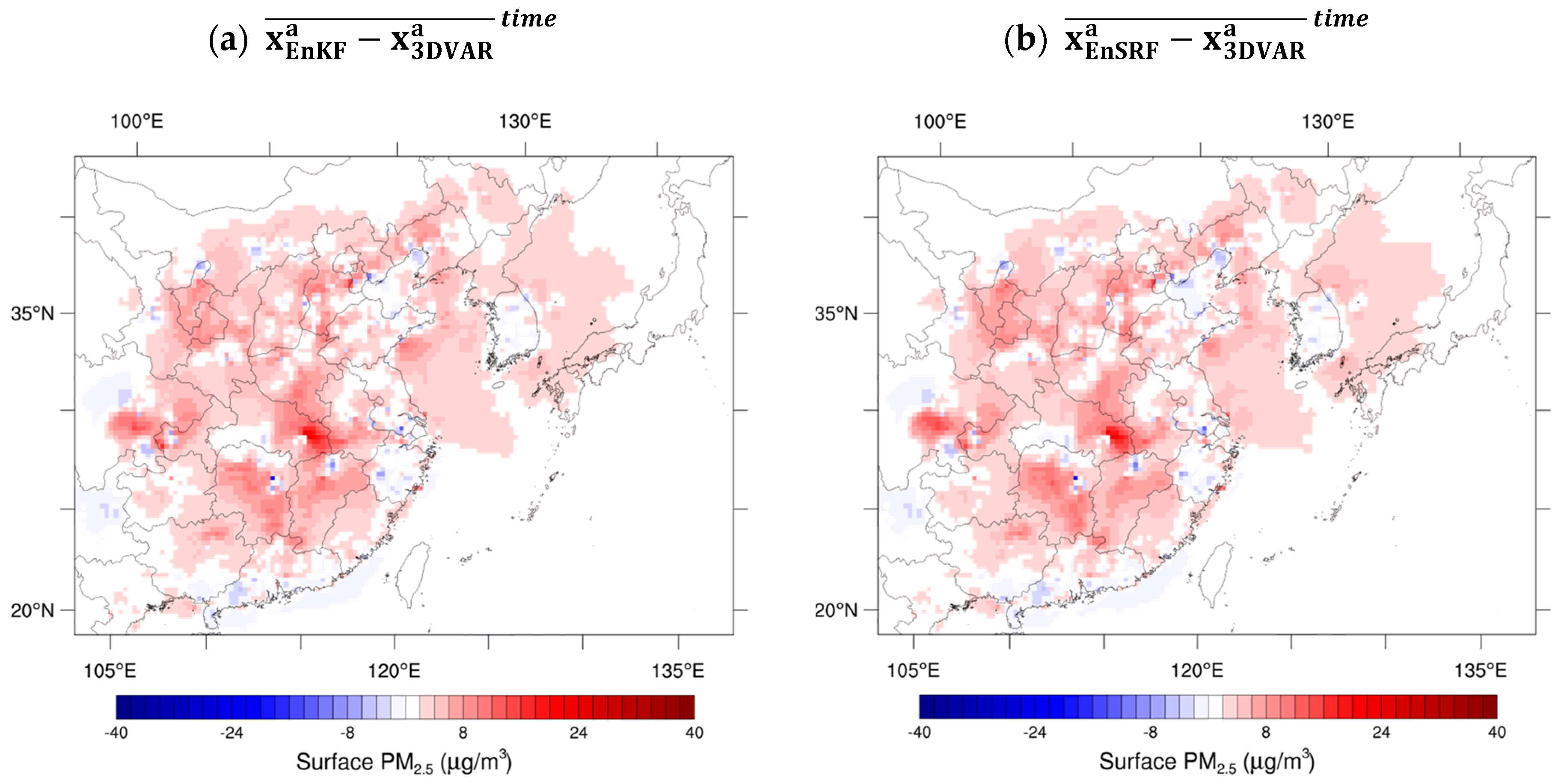
The difference in the analysis—an initial field improved through DA—was investigated for each DA method. Typically, analysis increments, i.e., analysis minus background, are used to investigate the impact of the assimilated observations. However, differentiating two analysis fields from different DA methods is also suitable to characterize not only the different impacts of observations on the improved initial conditions with respect to DA methods but also flow-dependent corrections using the ensemble-based DA. Figure 2 shows only the surface layer of the model by averaging differences in the analysis fields for different DA methods at each DA time point (168 times in total) for the entire period. The difference in the analysis field between the EnKF and EnSRF was very small, with an average of 0.01 μ g   m 3 (a maximum of 3.00 μ g   m 3 and a minimum of −2.28 μ g   m 3 ) in the surface layer. Therefore, only the difference between 3DVAR for EnKF and EnSRF is shown in Figure 2a,b, respectively. The difference in the concentration of the analysis field at the observation point was close to zero because the model errors at the point where the observation data were located were considered equally. The 3DVAR modified the initial field of the model to an isotropic shape based on the HLS set for the grid around the observation data; however, considering the EnKF and EnSRF, which are ensemble-based DAs, the observation data improved the model flow dependently. Thus, the area where the difference in the analysis field occurred appeared around the observation point. The average difference in the analytical field was 4–10 μ g   m 3 in the sea around the Korean Peninsula. This was reiterated by the absence of an observation point. The difference in the concentration of the analysis field had a positive value in most areas, which implied that EnKF or EnSRF predicted a higher value of PM2.5 compared with that of 3DVAR based on the transportation and diffusion for the prediction time after the DA (analysis time). The difference was greater in China, which had a higher concentration of PM2.5.

3.2. Length Scale Analysis and Relationships with Meteorological Variables

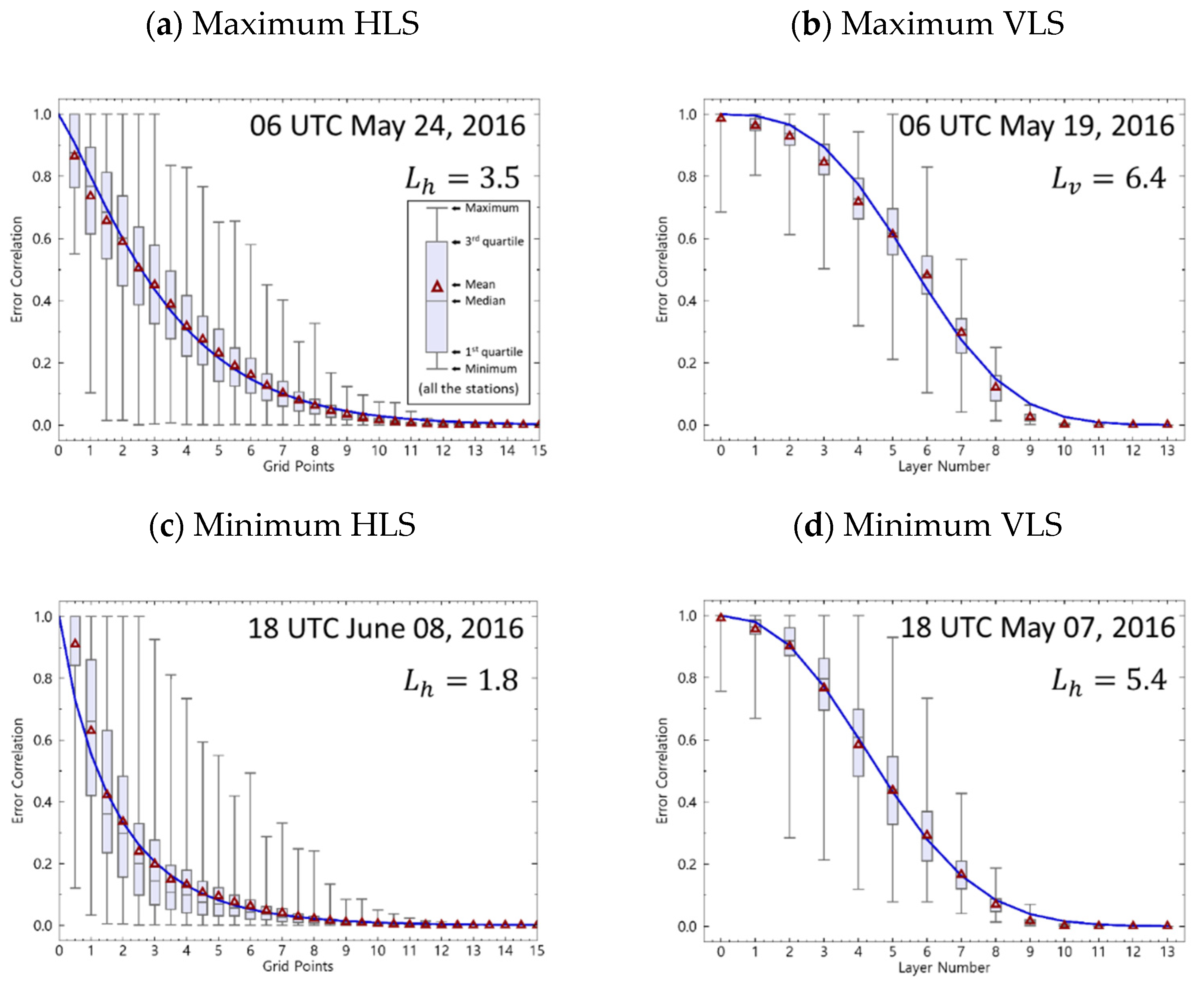
The HLS and VLS analyses of the BEC were performed to understand the difference between the analysis fields of the two ensemble-based methods and those of the 3DVAR discussed above. Figure 3 illustrates how much the error correlation of the model decreased with an increase in the distance of the horizontal grid distance away from the observation point and the number of vertical layers along the x-axis using the BEC of the EnKF. Only the results at the time when the estimated HLS and VLS recorded the minimum and maximum values are presented because the BEC was calculated every 6 h. Moreover, the results for all the observation points at the corresponding distance were used, and therefore, they were displayed using boxes and ticks to refer to the minimum, first quartile, median, third quartile, and maximum values. The solid blue line represents a function that best describes the average value; it includes both the HLS and VLS. For example, for the HLS, L h was 3.5 (for VLS, L v was 6.4). The effect of the ground observation value obtained via DA indicated that the error correlation of the model was reduced to e 1 in the surrounding 3.5 grid (6.4 upper layers). Further, it can be observed that the HLS had a very wide range of data at the corresponding grid distance because it included the results of all regions; the error correlation could be generated in a specific direction in the two-dimensional plane, which depended on the wind direction. This feature was unlike the features of the BEC of 3DVAR. Although the HLS range for the entire period was 1.8–3.5, that of the VLS was 5.4–6.4, and it indicated only a one-layer difference. However, considering the physical distance, HLS had a 48.6–94.5 km change in scale; the heights of the fifth, sixth, and seventh floors from the ground were 630, 980, and 1490 m, respectively. Therefore, the difference between 5.4 and 6.4 in VLS is an important difference in determining whether the effect of ground observation data affected only the lower layer of the whole planetary boundary layer. The EnSRF results of the same analysis are illustrated in Figure 4; the date and time when the maximum and minimum HLSs and VLSs were shown during the numerical experiment period were consistent. Although the difference between the VLS of EnSRF and that of EnKF was very small, the HLS of EnSRF showed a difference that was as large as the 0.4 grid distance compared with that of the EnKF. Considering the average difference for the entire DA time, the HLS of EnSRF was as large as the 0.25 grid distance compared with that of the EnKF. However, the VLS of the EnSRF was as high as 0.04 layers, which indicated that the influence of the observational data appeared in the horizontal direction because of the difference between the two DA methods.
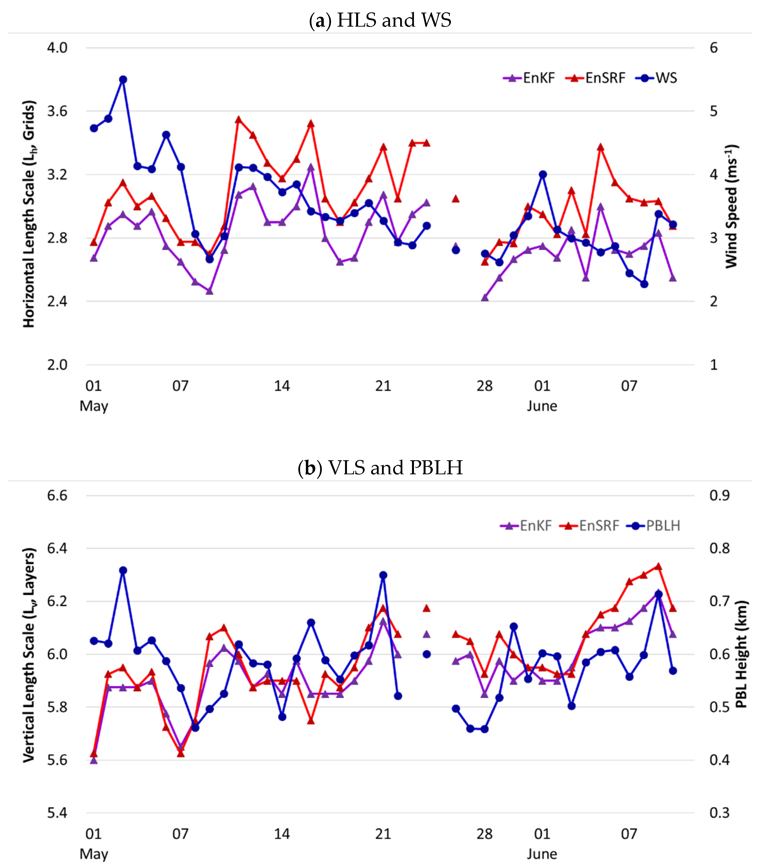
As shown in Figure 3 and Figure 4, the date and time when the maximum/minimum of the HLS or VLS appeared were different. The HLS was analyzed in association with the wind speed (WS) and the VLS was analyzed in association with the planetary boundary layer height (PBLH) because the causes of this difference may be attributed to meteorological factors. Changes in the daily average HLS, VLS, WS, and PBLH are shown in Figure 5. The dates 23 and 25 May and 11 June were excluded because all ground observation data of China were missing more than twice out of the four DAs daily. The average of all points of the daily average WS tended to significantly decrease until 9 May, followed by an increase and a gradual decrease (Figure 4a). The tendency of the HLS to change was closely related to these fluctuations in the WS; the HLS of EnSRF was consistently larger than that of EnKF. Figure 4b shows changes in the daily average VLS and PBLH at all points. From May to June, the altitude of the boundary layer tended to gradually increase as summer approached and the solar radiation became stronger. From 7 to 10 May, precipitation appeared as the low-pressure system passed from China to Korea; therefore, the altitude of the boundary layer decreased and subsequently increased. On 27 and 28 May, the altitude of the boundary layer decreased because of the precipitation in central and southern China. Owing to these daily changes, the VLS increased or decreased, i.e., the VLS continued to increase in early June, which was less than the difference between the HLS of EnSRF and that of EnKF. However, the difference widened in early June when the VLS increased compared with that in May.
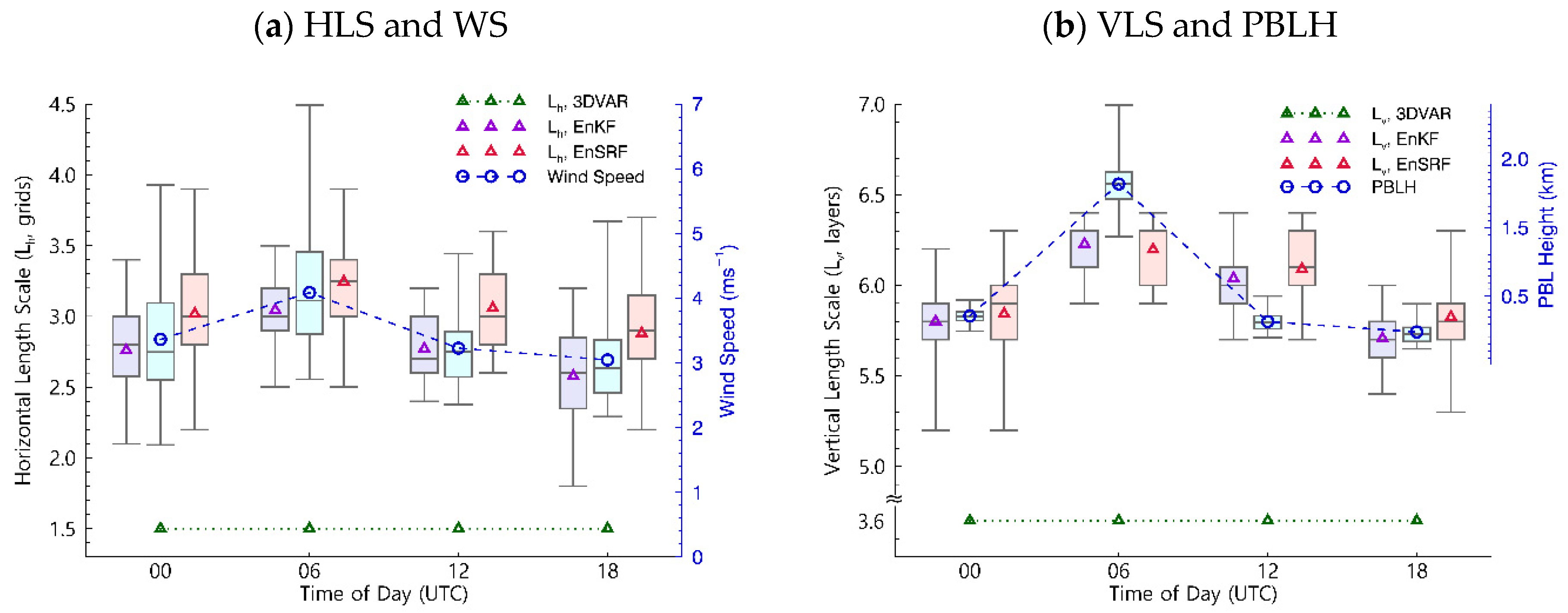
The average diurnal variation in the HLS and VLS is presented in Figure 6 to examine the horizontal/vertical correlation between day and night model errors. The HLS was analyzed using the daily change in WS; the VLS was analyzed using the daily change in PBLH. The box plot displays the data distribution for 42 days after taking the average of all points, showing the minimum, first quartile, median, third quartile, and maximum values from the bottom. The symbol represents an average of 42 days. The results are displayed at the bottom of the graph to compare the length scale values of the 3DVAR derived from the NMC. Further, 00 and 06 UTC correspond to daytime in China (08 and 14 in local time) and Korea (09 and 15 in local time), and 12 and 18 UTC corresponds to nighttime. Both WS and PBLH showed the highest values at midday and appeared low at night when the atmosphere was stabilized. This daily change tendency of the weather variables was consistent with that of the HLS and VLS. As indicated earlier, the length scale of the EnSRF was larger than that of the EnKF; the difference was noticeable in the HLS. Further, the length scale difference between the two DA methods increased at night compared with that during daytime. The length scale of 3DVAR was very small compared with those of the EnKF and EnSRF. The HLS of 3DVAR, which can be observed from the BEC diagnostic results provided by the GSI package, was a 1.5 grid distance, approximately half of the overall mean values of EnKF and EnSRF (2.79 and 3.05, respectively). The VLS had 3.6 layers in the 3DVAR. However, the EnKF and EnSRF averaged 5.94 and 5.99 layers, respectively, which indicates that the effect of the ground observation data on the upper layer could be limited in the 3DVAR. Further, this suggests that the difference between the analytical field of the variational method (3DVAR) and the ensemble-based method (EnKF and EnSRF) examined in Figure 2 was attributed to the difference between HLS and VLS.

3.3. Short-Term Predictions and Vertical Length Scale Adjustment for the 3DVAR

The results were compared with the observation results to examine how the characteristics of the analyzed length scale affected the DA performance. The short-term PM2.5 prediction performance was evaluated based on the results of prediction times (from +01 h to +06 h) because the DA was performed four times a day. Further, the tendency of daily concentration change in PM2.5 may be different because there was a difference in the time zone between China and Korea alongside the weather conditions based on sunrise and sunset. Thus, the prediction performance presented only the model results corresponding to the observation points in Korea.
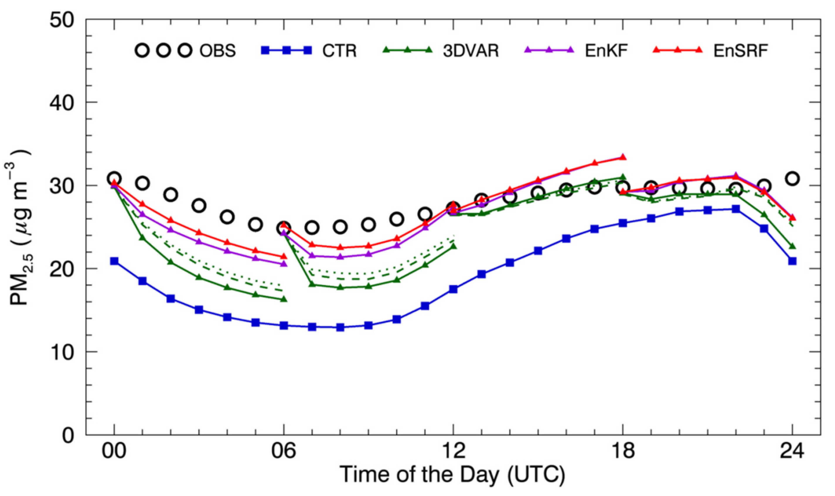
Figure 7 shows the diurnal variation in the PM2.5, averaged for 169 stations and 6 weeks in Korea. Along with the observed values, the results of the 3DVAR, EnKF, and EnSRF in the experiments where DA was not performed and those where DA was performed at 6 h intervals are displayed simultaneously. The PM2.5 tended to decrease during the daytime (00 and 06 UTC) because the boundary layer altitude increased after sunrise and the wind speed became stronger. Furthermore, a weak wind speed and low boundary layer altitude appeared because the atmosphere became stable after sunset; PM2.5 tended to increase again at night (12 and 18 UTC). These characteristics could be confirmed in the observations, and they were more clearly reflected in the model. The average concentration was underestimated when DA was not performed (CTR experiment) because not all emission sources were considered, the emission calculation methods were inaccurate, and there was uncertainty in the generation/destruction mechanism of the aerosol. Through DA, these errors were improved in all techniques. Although the predictability of the 3DVAR in the daytime was better than that of the CTR, its predictability was less than that of the EnKF and EnSRF. The improved initial fields at 00 UTC and 06 UTC through the 3DVAR DA tended to approach the CTR because the effects of the improved ICs disappeared rapidly. In contrast, the initial fields of 00 and 06 UTC for the EnKF and EnSRF exhibited very little bias at approximately 06 and 12 UTC; these were +06 h predictions, and the effect persisted. The predictability of the EnSRF was slightly better than that of the EnKF; however, the difference was insignificant. Hence, the two ensemble-based DA methods exhibited similar performances.
We confirmed that the cause of the rapid disappearance of the influence of the analysis fields of 3DVAR was the low VLS value. Therefore, the DA was additionally performed by increasing the VLS of 3DVAR to approximately six layers, which was the average value in the ensemble DA method. Figure 7 shows the results of performing 3DVAR with 1.5 and 2.0 times the VLS calculated by the NMC method. The most notable change shown after adjusting by 1.5 and 2.0 times was the improvement in the short-term prediction performance during the daytime. Because of the increased VLS, the influence of the ground observation data on the analytical sites of 00 and 06 UTC affected up to the altitude of the boundary layer, which spread to the surrounding areas through the process of transportation and diffusion at the prediction time, thereby enabling the prediction of PM2.5 to be close to the observation.
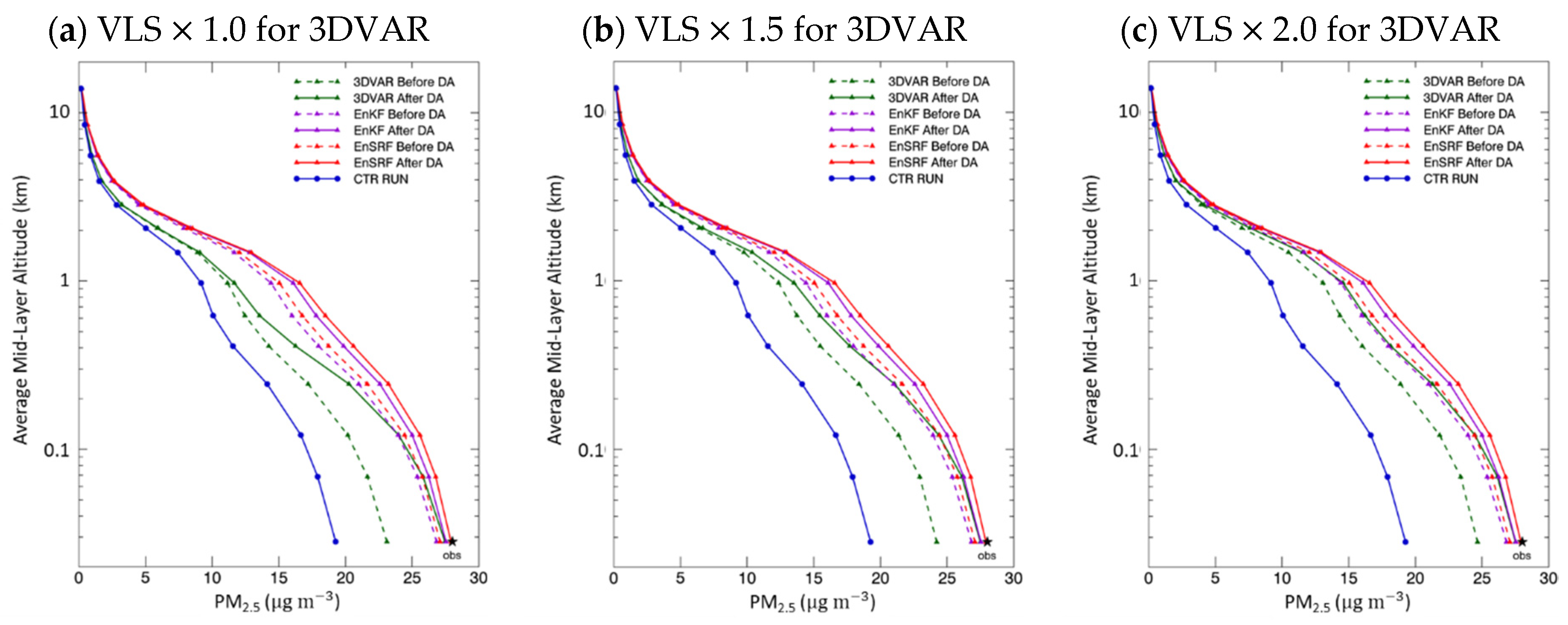
The average PM2.5 vertical distribution at all observation points was analyzed to investigate changes in the upper boundary layer in the analytical field (Figure 8). Along with the results of the CTR, the +06 h prediction (dotted line) results and +00 h analysis (solid line) results for each DA method are displayed simultaneously to identify the changes in the distribution of the vertical PM2.5 before and after the DA. Considering the results of the nonadjusted VLS of the 3DVAR (Figure 8a), the ground analysis value was close to the average observation concentration and shows the same value as that of the EnKF and EnSRF. However, the analysis profile showed a lower concentration distribution compared with those of the two ensemble-based DAs from approximately 200 to 1000 m. The analysis profile (solid green line) of 3DVAR gradually approached the ensemble DA experiment because the VLS was increased (Figure 8b,c). Accordingly, the distribution of the predicted concentration of +06 h was increased, and it approached the observed concentration on the ground, which resulted in improved predictability. The increase in the concentration from the dotted to the solid line was the average analysis increment at the time of the DA. The analysis increments of EnKF and EnSRF were lower because of the accumulated DA effect, whereas 3DVAR using the basic values of VLS showed poor short-term predictability, which indicated that significant increments were required.
The statistical analysis was performed at all times and points excluding 00, 06, 12, and 18 UTC when the DA was performed. This means that the observation data at the prediction time from +01 h to +06 h were used for statistical evaluations with independent observations over time. The results are summarized in Table 2. The definitions of each statistical metric are presented in the table below. When DA was applied instead of CTR, the figures improved for all metrics. The ensemble DA performed better than 3DVAR, and the EnSRF showed slightly better results than that of EnKF. An error of −30.7% was observed before the DA was applied considering the mean bias normalized by the mean concentration of the observed PM2.5 (normalized mean bias (NMB)) in Korea. However, the errors were systematically reduced to −13.0%, −4.4%, and −2.5% because 3DVAR, EnKF, and EnSRF were applied, respectively. There was also a systematic improvement in all the statistical metrics because the VLS of 3DVAR was applied 1.5 and 2.0 times. This implies that the VLS may be underestimated and needs to be when the BEC is estimated using the NMC method and applied to the 3DVAR. However, even the experiment with double VLS did not outperform the two ensemble-based DA methods.

4. Discussion

A length-scale analysis was performed to investigate the BEC characteristics of the EnKF and EnSRF, and the DA methods of the ensemble-based KF. The length scale diagnosed in the NMC method for calculating the BEC of the 3DVAR—a variational DA—was compared, and the correlation with the meteorological variables was examined. The difference in the analysis fields was negligible at ground observation points because the inflation of the Kalman filter was applied based on the 3DVAR’s model error variance. However, it was noticeable in the surrounding areas, especially over the sea.
The results of the length scale analysis in the Gaussian function fitting method indicated that the HLS showed an average of 2.788 and 3.050 grids for the EnKF and EnSRF, respectively. This implied that the EnSRF had a wider impact on the observation data. Considering the VLS, the EnKF averaged 5.943 and EnSRF 5.989 layers, which suggests that was no significant difference between the two DA methods; the ground observation data were significantly corrected to approximately 600 m, i.e., the sixth layer. For the two ensemble-based DA methods, the HLS showed a high correlation with the ground WS, and the VLS showed a high correlation with the PBLH for diurnal and daily variations. This result implies that the DA could be performed by applying “errors of today”, reflecting the weather conditions at the time of the DA when estimating the BEC through an ensemble prediction.
Our results confirmed a clear behavior of flow-dependent BEC in the CTM, whereas previous studies examined the predictability using DA techniques. The 6 h PM2.5 prediction results performed for 42 days were evaluated simultaneously for the CTR without DA, 3DVAR, EnKF, and EnSRF. Although all DA experiments significantly reduced the negative bias compared with CTR, EnKF and EnSRF showed superior performances. Further, the VLS of 3DVAR was lower than that of the two ensemble DA methods with 3.6 layers; therefore, the sensitivity to short-term predictability evaluation was investigated further by increasing the VLS. The uncontrolled experiments showed an NMB of −13.0%, whereas the predictability increased to −10.9% and −9.8% when the VLS was applied 1.5 and 2.0 times. This was a low bias compared with the CTR of −30.7%; however, it fell short of the EnKF and EnSRF of −4.4% and −2.5%, respectively. This implied that the horizontal flow-dependent characteristic differences were also important. In terms of the VLS for 3DVAR, we suggest that the VLS should be two times larger than that estimated by the NMC method based on our sensitivity simulations.
The length scale analysis method presented in this study is a simple method for finding a Gaussian function that best describes the error correlation of the BEC based on the physical distance. However, the GSI’s gen_be program estimates the length scale by directly solving the Gaussian function [33]. Although there were differences in the analysis methods in this study, it is more appropriate to apply the best-fitting method because various BECs were calculated for each scenario using the ensemble-based DA. Thus, the results of this study were not limited to predictability comparisons based on DA methods.
The results were significant in providing crucial basic information because they presented a correlation between meteorological variables and the scale analysis of the BEC, which is the core of the DA technology. However, it is necessary to use the same estimation method for direct comparison through strict length scale analysis. We plan to evaluate the predictability based on the DA method through a long-term prediction longer than the 6 h prediction (e.g., 24 h or 48 h) considered in this study. Other approaches for dimension-reduced DA other than the EnKF can be used for the CTM applications to reduce the sampling error, such as the reduced rank square root filter (RRSQRT) [45], singular evolutive Kalman filter (SEEK) [46], Karhunen–Loeve-based Kalman filter (KLKF) [47], and EnKF based on generalized polynomial chaos (gPC) [48]. In particular, to capture non-Gaussian features in a nonlinear model, dynamically orthogonal (DO) field equations [49], a mixture ensemble filter (MEnF) [50], and polynomial chaos expansion (PCE) [51] can be promising advanced DA techniques using the Gaussian mixture model (GMM) for the dimension-reduced methods. Furthermore, we plan to improve the PM2.5 predictability by applying a hybrid DA that combines the advantages of the ensemble-based DA (i.e., time-evolving forecast errors) and those of the 3DVAR by calculating the analysis fields using a variational method [28].

Author Contributions

Conceptualization, S.-Y.P.; methodology, S.-Y.P. and J.Y.; software, U.K.D. and J.Y.; validation, U.K.D.; formal analysis, S.-Y.P. and J.Y.; investigation, U.K.D. and J.Y.; writing—original draft preparation, S.-Y.P.; writing—review and editing, S.-Y.P. and U.K.D.; visualization, U.K.D.; supervision, S.-Y.P. All authors have read and agreed to the published version of the manuscript.

Funding

This research was supported by the National Research Foundation of Korea (NRF) funded by the Korean Government’s Ministry of Education (2020R1A6A1A03044834) and Ministry of Science, ICT and Future Planning (2019R1C1C1007997).

Institutional Review Board Statement

Not applicable.

Informed Consent Statement

Not applicable.

Data Availability Statement

The data presented in this study are available on request from the corresponding author.

Conflicts of Interest

The authors declare no conflict of interest. The funders had no role in the design of the study; in the collection, analyses, or interpretation of data; in the writing of the manuscript; or in the decision to publish the results.

Glossary

Data assimilationDA
Chemical transport modelCTM
Three- and four-dimensional variational methods3DVAR and 4DVAR
Optimal interpolationOI
Ensemble Kalman filterEnKF
Ensemble square root filterEnSRF
Local ensemble transform Kalman filter LETKF
Ensemble adjustment Kalman filter EAKF
Background error covariance BEC
National Meteorological CentreNMC
Hydrogen chlorideHCL
Nitric acidHNO3
Initial conditionIC
Boundary conditionBC
Community multiscale air qualityCMAQ
Horizontal and vertical length scaleHLS and VLS
Grid-point statistical interpolationGSI
National Centers for Environmental PredictionNCEP
Generalized background error covariance matrix modelGEN_BE
Relaxation-to-prior (or previous) spreadRTPS
NCEP FinalFNL
National Ambient Air Quality Monitoring Information System NAMIS
Korea-United States Air QualityKORUS-AQ
Control runCTR
Wind speedWS
Planetary boundary layer heightPBLH
Root mean square errorRMSE
Normalized mean biasNMB
Index of agreementIOA
Correlation coefficientCORR
Reduced rank square root filterRRSQRT
Singular evolutive Kalman filterSEEK
Karhunen–Loeve-based Kalman filterKLKF
Generalized polynomial chaosgPC
Dynamically orthogonalDO
Mixture ensemble filterMEnF
Polynomial chaos expansionPCE
Gaussian mixture modelGMM

References

  1. Sandu, A.; Chai, T. Chemical data assimilation—An overview. Atmosphere 2011, 2, 426–463. [Google Scholar] [CrossRef] [Green Version]
  2. Zhang, Y.; Bocquet, M.; Mallet, V.; Seigneur, C.; Baklanov, A. Real-time air quality forecasting, part II: State of the science, current research needs, and future prospects. Atmos. Environ. 2012, 60, 656–676. [Google Scholar] [CrossRef]
  3. Bocquet, M.; Elbern, H.; Eskes, H.; Hirtl, M.; Žabkar, R.; Carmichael, G.R.; Flemming, J.; Inness, A.; Pagowski, M.; Pérez Camaño, J.L.; et al. Data assimilation in atmospheric chemistry models: Current status and future prospects for coupled chemistry meteorology models. Atmos. Chem. Phys. 2015, 15, 5325–5358. [Google Scholar] [CrossRef] [Green Version]
  4. Menut, L.; Bessagnet, B. What can we expect from data assimilation for air quality forecast? Part I: Quantification with academic test cases. J. Atmos. Ocean. Technol. 2019, 36, 269–279. [Google Scholar] [CrossRef]
  5. Chai, T.; Kim, H.-C.; Pan, L.; Lee, P.; Tong, D. Impact of moderate resolution imaging spectroradiometer aerosol optical depth and AirNow PM2.5 assimilation on community multi-scale air quality aerosol predictions over the contiguous United States. J. Geophys. Res. Atmos. 2017, 122, 5399–5415. [Google Scholar] [CrossRef]
  6. Lee, K.; Yu, J.; Lee, S.; Park, M.; Hong, H.; Park, S.Y.; Choi, M.; Kim, J.; Kim, Y.; Woo, J.H.; et al. Development of Korean air quality prediction system version 1 (KAQPS v1) with focuses on practical issues. Geosci. Model Dev. 2020, 13, 1055–1073. [Google Scholar] [CrossRef] [Green Version]
  7. Pang, J.; Liu, Z.; Wang, X.; Bresch, J.; Ban, J.; Chen, D.; Kim, J. Assimilating AOD retrievals from GOCI and VIIRS to forecast surface PM2.5 episodes over Eastern China. Atmos. Environ. 2018, 179, 288–304. [Google Scholar] [CrossRef]
  8. Ha, S.; Liu, Z.; Sun, W.; Lee, Y.; Chang, L. Improving air quality forecasting with the assimilation of GOCI aerosol optical depth (AOD) retrievals during the KORUS-AQ period. Atmos. Chem. Phys. 2020, 20, 6015–6036. [Google Scholar] [CrossRef]
  9. Zhang, Z.; Zang, Z.; Cheng, X.; Lu, C.; Huang, S.; Hu, Y.; Liang, Y.; Jin, L.; Ye, L. Development of three-dimensional variational data assimilation method of aerosol for the CMAQ model: An application for PM2.5 and PM10 forecasts in the Sichuan Basin. Earth Space Sci. 2021, 8, e2020EA001614. [Google Scholar] [CrossRef]
  10. Morcrette, J.J.; Boucher, O.; Jones, L.; Salmond, D.; Bechtold, P.; Beljaars, A.; Benedetti, A.; Bonet, A.; Kaiser, J.W.; Razinger, M.; et al. Aerosol analysis and forecast in the European centre for medium-range weather forecasts integrated forecast system: Forward modeling. J. Geophys. Res. Atmos. 2009, 114, D06206. [Google Scholar] [CrossRef]
  11. Benedetti, A.; Di Giuseppe, F.; Jones, L.; Peuch, V.H.; Rémy, S.; Zhang, X. The value of satellite observations in the analysis and short-range prediction of Asian dust. Atmos. Chem. Phys. 2019, 19, 987–998. [Google Scholar] [CrossRef] [Green Version]
  12. Lopez-Restrepo, S.; Yarce, A.; Pinel, N.; Quintero, O.L.; Segers, A.; Heemink, A.W. Forecasting PM10 and PM2.5 in the Aburrá Valley (Medellín, Colombia) via EnKF based data assimilation. Atmos. Environ. 2020, 232, 117507. [Google Scholar] [CrossRef]
  13. Park, S.Y.; Dash, U.K.; Yu, J.; Yumimoto, K.; Uno, I.; Song, C.H. Implementation of an ensemble Kalman filter in the community multiscale air quality model (CMAQ Model v5.1) for data assimilation of ground-level PM2.5. Geosci. Model Dev. Discuss. 2021, 2021, 1–35. [Google Scholar] [CrossRef]
  14. Chu, K.; Peng, Z.; Liu, Z.; Lei, L.; Kou, X.; Zhang, Y.; Bo, X.; Tian, J. Evaluating the impact of emissions regulations on the emissions reduction during the 2015 China victory day parade with an ensemble square root filter. J. Geophys. Res. Atmos. 2018, 123, 4122–4134. [Google Scholar] [CrossRef]
  15. Choi, Y.; Chen, S.-H.; Huang, C.-C.; Earl, K.; Chen, C.-Y.; Schwartz, C.S.; Matsui, T. Evaluating the impact of assimilating aerosol optical depth observations on dust forecasts over North Africa and the East Atlantic using different data assimilation methods. J. Adv. Model. Earth Syst. 2020, 12, e2019MS001890. [Google Scholar] [CrossRef] [PubMed] [Green Version]
  16. Yumimoto, K.; Nagao, T.M.; Kikuchi, M.; Sekiyama, T.T.; Murakami, H.; Tanaka, T.Y.; Ogi, A.; Irie, H.; Khatri, P.; Okumura, H.; et al. Aerosol data assimilation using data from Himawari-8, a next-generation geostationary meteorological satellite. Geophys. Res. Lett. 2016, 43, 5886–5894. [Google Scholar] [CrossRef]
  17. Kong, L.; Tang, X.; Zhu, J.; Wang, Z.; Li, J.; Wu, H.; Wu, Q.; Chen, H.; Zhu, L.; Wang, W.; et al. A 6-year-long (2013–2018) high-resolution air quality reanalysis dataset in China based on the assimilation of surface observations from CNEMC. Earth Syst. Sci. Data 2021, 13, 529–570. [Google Scholar] [CrossRef]
  18. Rubin, J.I.; Reid, J.S.; Hansen, J.A.; Anderson, J.L.; Collins, N.; Hoar, T.J.; Hogan, T.; Lynch, P.; McLay, J.; Reynolds, C.A.; et al. Development of the ensemble navy aerosol analysis prediction system (ENAAPS) and its application of the data assimilation research testbed (DART) in support of aerosol forecasting. Atmos. Chem. Phys. 2016, 16, 3927–3951. [Google Scholar] [CrossRef] [Green Version]
  19. Ma, C.; Wang, T.; Mizzi, A.P.; Anderson, J.L.; Zhuang, B.; Xie, M.; Wu, R. Multiconstituent data assimilation with WRF-Chem/DART: Potential for adjusting anthropogenic emissions and improving air quality forecasts over Eastern China. J. Geophys. Res. Atmos. 2019, 124, 7393–7412. [Google Scholar] [CrossRef]
  20. Kalnay, E. Atmospheric Modeling, Data Assimilation and Predictability; Cambridge University Press: Cambridge, UK, 2002. [Google Scholar]
  21. Parrish, D.F.; Derber, J.C. The National Meteorological Center’s spectral statistical-interpolation analysis system. Mon. Weather Rev. 1992, 120, 1747–1763. [Google Scholar] [CrossRef]
  22. Pagowski, M.; Grell, G.A. Experiments with the assimilation of fine aerosols using an ensemble Kalman filter. J. Geophys. Res. Atmos. 2012, 117, D21302. [Google Scholar] [CrossRef]
  23. Skachko, S.; Errera, Q.; Ménard, R.; Christophe, Y.; Chabrillat, S. Comparison of the ensemble Kalman filter and 4D-Var assimilation methods using a stratospheric tracer transport model. Geosci. Model Dev. 2014, 7, 1451–1465. [Google Scholar] [CrossRef] [Green Version]
  24. Chatterjee, A.; Michalak, A.M. Technical note: Comparison of ensemble Kalman filter and variational approaches for CO2 data assimilation. Atmos. Chem. Phys. 2013, 13, 11643–11660. [Google Scholar] [CrossRef] [Green Version]
  25. Peng, Z.; Liu, Z.; Chen, D.; Ban, J. Improving PM2.5 forecast over China by the joint adjustment of initial conditions and source emissions with an ensemble Kalman filter. Atmos. Chem. Phys. 2017, 17, 4837–4855. [Google Scholar] [CrossRef] [Green Version]
  26. Peng, Z.; Lei, L.; Liu, Z.; Sun, J.; Ding, A.; Ban, J.; Chen, D.; Kou, X.; Chu, K. The impact of multi-species surface chemical observation assimilation on air quality forecasts in China. Atmos. Chem. Phys. 2018, 18, 17387–17404. [Google Scholar] [CrossRef] [Green Version]
  27. Evensen, G. The ensemble Kalman Filter: Theoretical formulation and practical implementation. Ocean Dyn. 2003, 53, 343–367. [Google Scholar] [CrossRef]
  28. Schwartz, C.S.; Liu, Z.; Lin, H.-C.; Cetola, J.D. Assimilating aerosol observations with a “hybrid” variational-ensemble data assimilation system. J. Geophys. Res. Atmos. 2014, 119, 4043–4069. [Google Scholar] [CrossRef]
  29. Chen, D.; Liu, Z.; Ban, J.; Zhao, P.; Chen, M. Retrospective analysis of 2015–2017 wintertime PM2.5 in China: Response to emission regulations and the role of meteorology. Atmos. Chem. Phys. 2019, 19, 7409–7427. [Google Scholar] [CrossRef] [Green Version]
  30. Whitaker, J.S.; Hamill, T.M. Ensemble data assimilation without perturbed observations. Mon. Weather Rev. 2002, 130, 1913–1924. [Google Scholar] [CrossRef]
  31. Shao, H.; Derber, J.; Huang, X.-Y.; Hu, M.; Newman, K.; Stark, D.; Lueken, M.; Zhou, C.; Nance, L.; Kuo, Y.-H.; et al. Bridging research to operations transitions: Status and plans of community GSI. Bull. Am. Meteor. Soc. 2016, 97, 1427–1440. [Google Scholar] [CrossRef]
  32. Lee, S.; Song, C.H.; Han, K.M.; Henze, D.K.; Lee, K.; Yu, J.; Woo, J.H.; Jung, J.; Choi, Y.; Saide, P.E.; et al. Impacts of uncertainties in emissions on aerosol data assimilation and short-term PM2.5 predictions over Northeast Asia. Atmos. Environ. 2022, 271, 11921. [Google Scholar] [CrossRef]
  33. Descombes, G.; Auligné, T.; Vandenberghe, F.; Barker, D.M.; Barré, J. Generalized background error covariance matrix model (GEN_BE v2.0). Geosci. Model Dev. 2015, 8, 669–696. [Google Scholar] [CrossRef] [Green Version]
  34. Gaspari, G.; Cohn, S.E. Construction of correlation functions in two and three dimensions. Q. J. R. Meteor. Soc. 1999, 125, 723–757. [Google Scholar] [CrossRef]
  35. Constantinescu, E.M.; Sandu, A.; Chai, T.; Carmichael, G.R. Assessment of ensemble-based chemical data assimilation in an idealized setting. Atmos. Environ. 2007, 41, 18–36. [Google Scholar] [CrossRef]
  36. Whitaker, J.S.; Hamill, T.M. Evaluating methods to account for system errors in ensemble data assimilation. Mon. Weather Rev. 2012, 140, 3078–3089. [Google Scholar] [CrossRef]
  37. Skamarock, W.C.; Klemp, J.; Dudhia, J.; Gill, D.O.; Barker, D.; Wang, W.; Powers, J.G. A description of the advanced research WRF version 3 (No. NCAR/TN-475+STR). Univ. Corp. Atmos. Res. 2008, 27, 3–27. [Google Scholar] [CrossRef]
  38. National Centers for Environmental Prediction/National Weather Service/NOAA/U.S. Department of Commerce. NCEP FNL Operational Model Global Tropospheric Analyses, Continuing from July 1999; Research Data Archive at the National Center for Atmospheric Research, Computational and Information Systems Laboratory: Boulder, CO, USA, 2000. [Google Scholar] [CrossRef]
  39. Byun, D.; Schere, K.L. Review of the governing equations, computational algorithms, and other components of the models-3 community multiscale air quality (CMAQ) modeling system. Appl. Mech. Rev. 2006, 59, 51–77. [Google Scholar] [CrossRef]
  40. Jang, Y.; Lee, Y.; Kim, J.; Kim, Y.; Woo, J.-H. Improvement China point source for improving bottom-up emission inventory. Asia-Pac. J. Atmos. Sci. 2020, 56, 107–118. [Google Scholar] [CrossRef]
  41. Guenther, A.; Karl, T.; Harley, P.; Wiedinmyer, C.; Palmer, P.I.; Geron, C. Estimates of global terrestrial isoprene emissions using MEGAN (Model of Emissions of Gases and Aerosols from Nature). Atmos. Chem. Phys. 2006, 6, 318–3210. [Google Scholar] [CrossRef] [Green Version]
  42. Guenther, A.B.; Jiang, X.; Heald, C.L.; Sakulyanontvittaya, T.; Duhl, T.; Emmons, L.K.; Wang, X. The model of emissions of gases and aerosols from nature version 2.1 (MEGAN2.1): An extended and updated framework for modeling biogenic emissions. Geosci. Model Dev. 2012, 5, 1471–1492. [Google Scholar] [CrossRef] [Green Version]
  43. Wiedinmyer, C.; Akagi, S.K.; Yokelson, R.J.; Emmons, L.K.; Al-Saadi, J.A.; Orlando, J.J.; Soja, A.J. The Fire inventory from NCAR (FINN): A high resolution global model to estimate the emissions from open burning. Geosci. Model Dev. 2011, 4, 625–641. [Google Scholar] [CrossRef] [Green Version]
  44. Jordan, C.E.; Crawford, J.H.; Beyersdorf, A.J.; Eck, T.F.; Halliday, H.S.; Nault, B.A.; Chang, L.-S.; Park, J.; Park, R.; Lee, G.; et al. Investigation of factors controlling PM2.5 variability across the South Korean Peninsula during KORUS-AQ. Elem. Sci. Anthr. 2020, 8, 28. [Google Scholar] [CrossRef] [PubMed]
  45. Verlaan, M.; Heemink, A.W. Tidal flow forecasting using reduced-rank square root filters. Stoch. Hydrol. Hydraul. 1997, 11, 349–368. [Google Scholar] [CrossRef] [Green Version]
  46. Pham, D.T.; Verron, J.; Roubaud, M.C. A singular evolutive extended kalman filter for data assimilation in oceanography. J. Mar. Syst. 1998, 16, 323–340. [Google Scholar] [CrossRef]
  47. Zhang, D.; Lu, Z.; Chen, Y. Dynamic reservoir data assimilation with an efficient, dimension-reduced Kalman filter. SPE J. 2007, 12, 108–117. [Google Scholar] [CrossRef]
  48. Li, J.; Xiu, D. A generalized polynomial chaos based ensemble Kalman filter with high accuracy. J. Comput. Phys. 2009, 228, 5454–5469. [Google Scholar] [CrossRef]
  49. Sondergaard, T.; Lermusiaux, P.F.J. Data assimilation with Gaussian mixture models using the dynamically orthogonal field equations. Part I: Theory and scheme. Mon. Weather Rev. 2013, 141, 1737–1760. [Google Scholar] [CrossRef] [Green Version]
  50. Tagade, P.; Seybold, H.; Ravela, S. Mixture ensembles for data assimilation in dynamic data-driven environmental systems. Procedia Comput. Sci. 2014, 29, 1266–1276. [Google Scholar] [CrossRef] [Green Version]
  51. Avasarala, S.; Subramani, D. A non-Gaussian Bayesian filter for sequential data assimilation with non-intrusive polynomial chaos expansion. Int. J. Numer. Methods Eng. 2021, 122, 7156–7181. [Google Scholar] [CrossRef]
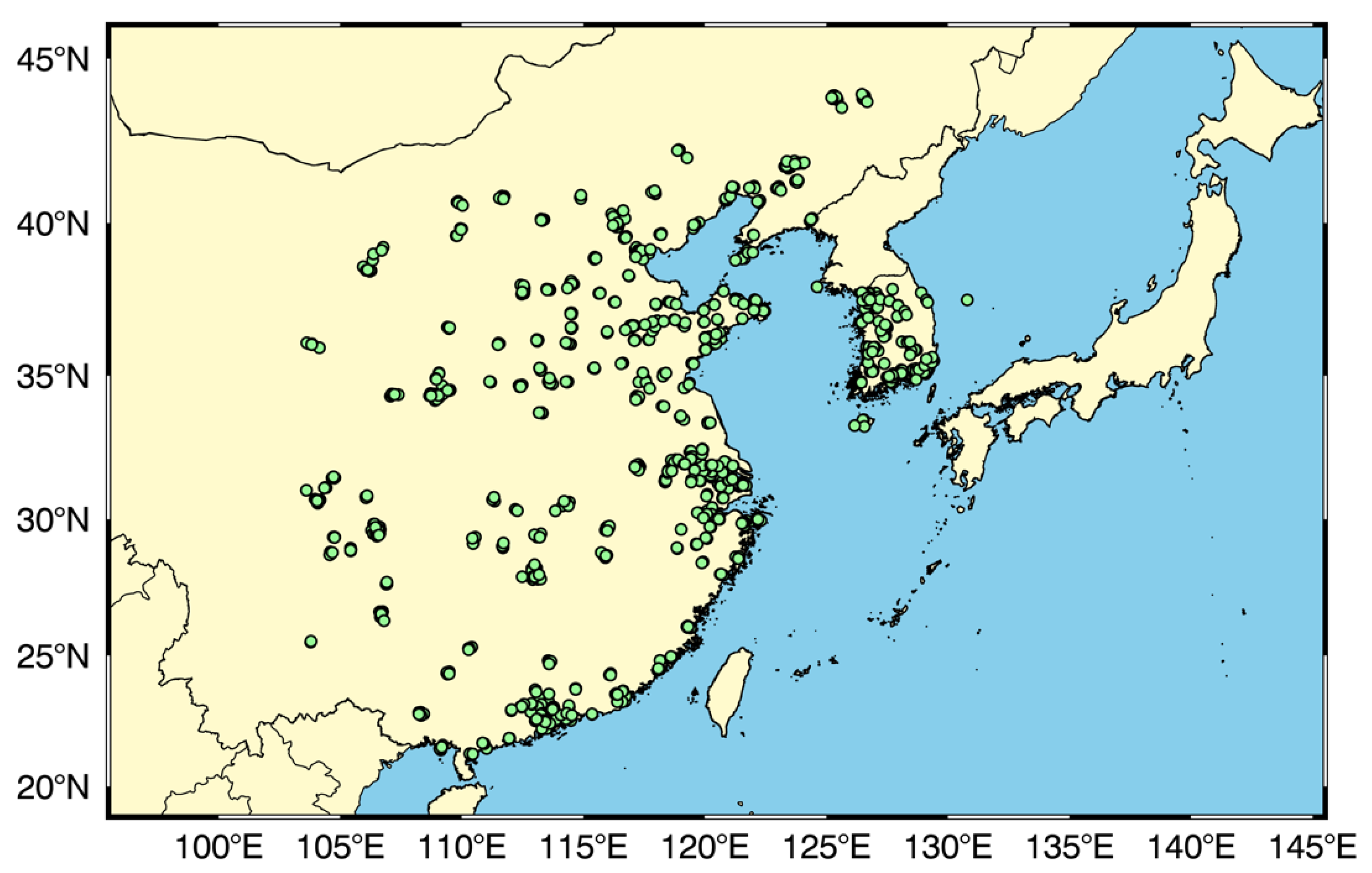
Figure 1. Numerical study domain in Northeast Asia. The green circles present the ground stations observing PM2.5; they are used in the data assimilations. The total number of stations in China and Korea is 762–790 and 133–165, respectively, depending on the missing time.
Atmosphere 13 00160 g001
Figure 2. Horizontal distributions for the mean differences in PM2.5 analytical fields: Differences between (a) EnKF and 3DVAR and (b) EnSRF and 3DVAR.
Atmosphere 13 00160 g002
Figure 3. Examples of the estimated horizontal ((a,c) Lh) and vertical ((b,d) Lv) length scales for the EnKF experiment when each value was the maximum (a,b) and the minimum (c,d). The x-axis indicates the grid points and layer numbers from the observation sites for Lh and Lv, respectively. The minimum, lower quartile, median, upper quartile, and maximum values from all samples’ corresponding distances are presented using whisker and box plots from the bottom. The blue lines indicate the function lines, which explain the mean values (red triangles).
Atmosphere 13 00160 g003
Figure 4. Same as Figure 3 (except for the EnSRF experiment).
Atmosphere 13 00160 g004
Figure 5. Daily variations in (a) the horizontal length scale versus wind speed and (b) the vertical length scale versus the PBL height for the EnKF and EnSRF.
Atmosphere 13 00160 g005
Figure 6. Diurnal variations in the horizontal length scales for 3DVAR, EnKF, and EnSRF with wind speed at each time of the day (a). Same as (a) but includes those of vertical length scales with the PBL height (b). The fixed-length scales estimated from the NMC method and used in 3DVAR are also shown.
Atmosphere 13 00160 g006
Figure 7. Diurnal variations in the mean PM2.5 at all observation sites in Korea during the simulation period and for the observed values (OBS), control run without DA (CTR), and experiments with DA (3DVAR, EnKF, and EnSRF). Two additional experiments for increasing the vertical length scale by 1.5 (dashed lines) and 2.0 (dotted lines) times are shown. There are two values for all DA experiments at the DA times (00(24), 06, 12, and 18 UTC) because of the discrete sequences for the DA procedure.
Atmosphere 13 00160 g007
Figure 8. Average vertical distributions of PM2.5 at all observation sites in Korea at all data assimilation times (00, 06, 12, and 18 UTC) for the CTR and DA (3DVAR, EnKF, and EnSRF) experiments. The results of increasing the vertical length scale (Lv) for the 3DVAR by (a) 1.0 (i.e., default value), (b) 1.5 and (c) 2.0 times. The dashed and solid lines for the DA experiments indicate the periods before and after the DA, which imply the background (or +06 h prediction) and analysis (or +00 h), respectively. The mean PM2.5 observed at the ground level is marked with star symbols.
Atmosphere 13 00160 g008
Table 1. Grid information and period for the WRF-CMAQ modeling system.
ModelWRF v3.8.1CMAQ v5.2.1
Horizontal grids153 × 114144 × 105
Grid resolution27 km27 km
Vertical layers33 layers (top: 50 hPa)15 layers (top: 20 km)
ICs and BCsNCEP FNL 0.25° dataDefault static profiles
Simulation period00 UTC 26 April 2016–00 UTC 12 June 2016,
including 5 days spin-up from the beginning
Table 2. Quantitative evaluation results obtained via the statistical metrics (mean, RMSE, NMB, IOA, and CORR). All metrics were calculated using hourly PM2.5 observations and models for each experiment during the 42 days of simulation, excluding the analytical time (00, 06, 12, and 18 UTC) for each day.
Metric *CTR3DVREnKFEnSRF
L v   ×   1.0 L v   ×   1.5 L v   ×   2.0
Mean **
( μ g   m 3 )
19.424.424.825.126.827.3
RMSE
( μ g   m 3 )
18.312.612.412.311.911.7
NMB
(%)
−30.7−13.0−10.9−9.8−4.4−2.5
IOA0.6860.8340.8420.8440.8520.861
CORR0.5280.7210.7270.7290.7350.735
* Mean: O ¯ = ( 1 / N ) i = 1 N O i and M ¯ = ( 1 / N ) i = 1 N M i , RMSE: ( 1 / N ) i = 1 N ( M i O i ) 2 , NMB: ( 1 / N ) i = 1 N ( M i O i ) / O ¯ × 100 , IOA: 1 i = 1 N ( M i O i ) 2 i = 1 N ( | M i O ¯ | + | O i O ¯ | ) 2 , and CORR: i = 1 N ( M i M ¯ ) ( O i O ¯ ) i = 1 N ( M i M ¯ ) 2 i = 1 N ( O i O ¯ ) 2 , where M and O represent the model and observation, respectively. ** The mean concentration in the observed data was 28.0 μ g   m 3 .
Publisher’s Note: MDPI stays neutral with regard to jurisdictional claims in published maps and institutional affiliations.