Abstract
Climate change and human activities have profoundly affected the world with extreme precipitation, heat waves, water scarcity, frequent floods and intense droughts. It is acknowledged that climate change will persist and perhaps intensify in the future, and it is thus meaningful to explore the quantitative impacts of these changes on hydrological regimes. The Jiulong River basin serves as an important watershed on the southeast coast of China. However, future hydrological changes under the combined impacts of climate change and land use change have been barely investigated. In this study, the climate outputs from five general circulation models (GCMs) under the Coupled Model Intercomparison Project Phase 6 (CMIP6) were corrected and spatially downscaled by a statistical downscaling method combining quantile mapping and machine learning. The future high-resolution land use maps were projected by the CA–Markov model with land use changes from the Land-Use Harmonization 2 (LUH2) as constraints. The future dynamic vegetation process was projected by the Biome-GBC model, and then, the future hydrological process under four representative concentration pathways and shared socioeconomic pathways (RCP–SSP) combined scenarios was simulated by a distributed hydrological model. Based on the copula method, the flood frequency and corresponding return periods were derived. The results demonstrated that future precipitation and air temperature would continue to rise, and future land use changes would have different developing pathways determined by the designs in various SSP–RCPs. Under the combined impacts of climate and land use change, the total available water resources will increase due to increasing precipitation, and the high flow and low flow will both increase at three stations under the four SSP–RCPs. The annual 1-day maximum discharge is projected to increase by 67–133% in the last decade of the 21st century, and the annual 7-day minimum discharge is projected to increase by 19–39%. The flood frequency analysis showed that the Jiulong River basin would face more frequent floods in the future. By the end of the 21st century, the station-average frequency of a historical 100-year flood will increase by 122% under the most optimistic scenario (SSP126) and increase by 213% under the scenario of greatest regional rivalry (SSP370). We demonstrated that climate change would be the major cause for the increase in future high flows and that land use change would dominate future changes in low flows. Finally, we recommend integrated and sustainable water management systems to tackle future challenges in this coastal basin.
1. Introduction
With socioeconomic developments, climate change and human activities have profoundly affected the hydrologic cycle around the world [1]. These changes have led to changes in the severity, frequency and duration of extreme events [2], including extreme heat waves [3], intense droughts [4] and recurrent flooding [5]. These extreme events may have a negative impact on biodiversity [6], crop yields [7], human health [2] and on various other socioeconomic factors [8]. Coastal areas typically have dense populations, concentrated urban construction and developed economies that are highly vulnerable to extreme floods [9,10]. Thus, it is imperative to explore the potential changes in future flow regimes by considering both climate change and human activities under global warming and socioeconomic development to formulate adaptation and mitigation strategies, especially for coastal basins [11].
Numerous studies have detected possible future changes in runoff under the impacts of climate and land use changes, and then analyzed with great detail the potential changes in different hydrological regimes including high and low flows. Most of them adopted hydrological models with projected future climate forcing data from general circulation models (GCMs) under the Coupled Model Intercomparison Project (CMIP) [12,13,14,15,16]. Based on a global river routing model with outputs of 11 GCMs from CMIP5, Hirabayashi et al. [14] projected future changes in runoff on a global scale and concluded that a warmer climate would significantly increase future high flows in Southeast Asia, peninsular India, eastern Africa and the northern half of the Andes. Meanwhile, their scenario analysis revealed that global flood risks will increase with climate warming. Using a distributed semi-physically based rainfall-runoff model with climate projections from CMIP5, Alfieri et al. [17] focused on the high flow changes and projected future flood frequency in Europe under warmer future conditions and concluded that flood peaks with return periods above 100 years would, on average, double in frequency within 3 decades. Rottler et al. [18] detected and assessed future changes in runoff in the Rhine River under various climate scenarios in CMIP5 with full consideration of basin hydrological processes by a mesoscale hydrologic model and demonstrated increases in high flow due to future increases in antecedent precipitation and temperature. With a calibrated hydrological model and UKCIP98 climate change scenarios, Arnell [19] explored the impact of climate change on low flows in Britain, and concluded that the larger variability in future climate would lead to a decrease in low flows and the degree of the impact would be greater in upland basins.
In addition to climate change, a large number of studies have proven that land use change has a significant impact on flow regimes [1,20,21,22]. Baker et al. [21] used the Soil and Water Assessment Tool (SWAT) to simulate the hydrological process of a small basin in Kenya under three different land use maps and explored the impacts of forest degradation and cropland expansion on the allocation of surface and groundwater recharge as well as ecological effects. Their results showed that deforestation would shift the allocation and have a negative ecological effect. With a process-based hydrological model, Li et al. [22] detected the effects of urbanization on various elements of the hydrological cycle and concluded that the increase in impervious surfaces and decrease in evapotranspiration caused by vegetation losses during rapid urbanization would lead to an increase in low flow, and eventually increase in water yield. Considering the impacts of land use change and climate change simultaneously, some studies projected future possible changes in hydrological processes at a watershed scale [1,23,24,25,26]. Tavakoli et al. [27] explored the response of extreme flows under the impacts of climate change and urban growth with a hydrological model, and concluded that extreme low flows would decrease noticeably due to climate change and be less sensitive to urban development, while extreme high flows would increase greatly due to both climate change and urban development. Using a hydrological model and a land use simulation model, Chacuttrikul et al. [24] assessed the impacts of climate and land use changes on river discharge in a small basin in Thailand and showed that the increase in future precipitation would lead to an increase in both low and high flows, and that continuous conversion from forest to paddy fields would cause an increase in both high and low flows. In addition, they concluded that land use change dominated historical runoff changes, while future discharge changes would be mainly caused by climate change. Similarly, Yang et al. [1] adopted the SWAT model to project future hydrological processes and the CA–Markov model to simulate future land use changes in the Luanhe River basin in China and projected future possible changes in runoff under continuous afforestation and global warming. They illustrated that climate change would increase the high flows and lead to a slight decrease in low flow seasons, and future afforestation would cause a reduction in low flows. In addition, some of the increase in runoff due to climate change would be offset by reduced runoff caused by afforestation, but climate change would still play a dominant factor in the future. Although the impacts of climate change and land use change on hydrological processes have been evaluated by many previous studies, most of the land use change scenarios are designed independently and are not consistent with climate change scenarios designed by CMIP. This deficiency may lead to a large bias in accurately reflecting future possible changes in hydrological regimes.
The newly released CMIP6 has set a series of more reasonable scenarios than previous scenarios designed in CMIP5. The new scenarios are rooted in socioeconomic trajectories and are named representative concentration pathways (RCPs) and shared socioeconomic pathways (SSPs) combined scenarios [28]. Serving as a required input of GCMs in CMIP6, Land-Use Harmonization 2 (LUH2) provides a newly harmonized annual land use dataset from 850 to 2100 under future SSP–RCP scenarios [29]. To detect future changes in hydrological processes, a physically based hydrological model is necessary, and the geomorphology-based hydrological model (GBHM) developed by Yang et al. [30] can be used for future hydrological projections. The GBHM model is a fully distributed hydrological model and has been successfully applied in many regions [31,32,33,34,35] including the Jiulong river basin. However, there is a gap between the required inputs and the data provided by CMIP6 and LUH2, which have systematic bias and coarse spatial resolution. To bridge this gap, statistical downscaling methods can effectively correct systematic bias and downscale the spatial resolution and are widely used for future climate downscaling [36,37,38]. The CA–Markov model is a popular and robust land use simulation model and can potentially be adopted for spatial downscaling of land use maps [1,39,40,41,42]. Combining the SSP–RCP scenario-based climate forcing from CMIP6 and land use maps from LUH2, it is possible to explore future water-related disaster changes considering greenhouse gas emissions and socioeconomic development simultaneously with the help of the GBHM and CA–Markov models.
In this study, we conducted climate downscaling using a statistical downscaling method and projected future high-resolution land use maps under various SSP–RCPs based on CA–Markov and LUH2. With future climate forcing and land use data, we projected future dynamic vegetation growth dynamics by a process-based ecosystem model and then simulated future hydrological responses in the Jiulong River basin. Based on these projections, we analyzed future changes in annual runoff and flow regimes which included high flows (annual 1-day maximum, 3-day maximum and 7-day maximum discharges) and low flows (annual 7-day minimum, 30-day minimum and 90-day minimum discharges), and calculated flood frequency using a copula-based method. We strived to (1) illustrate possible changes in future climate and land use; (2) demonstrate future changes in high and low flows under the combined impacts of climate and land use changes; and (3) provide corresponding suggestions to mitigate and adapt to future water-related risks.
2. Materials and Methods
2.1. Study Area
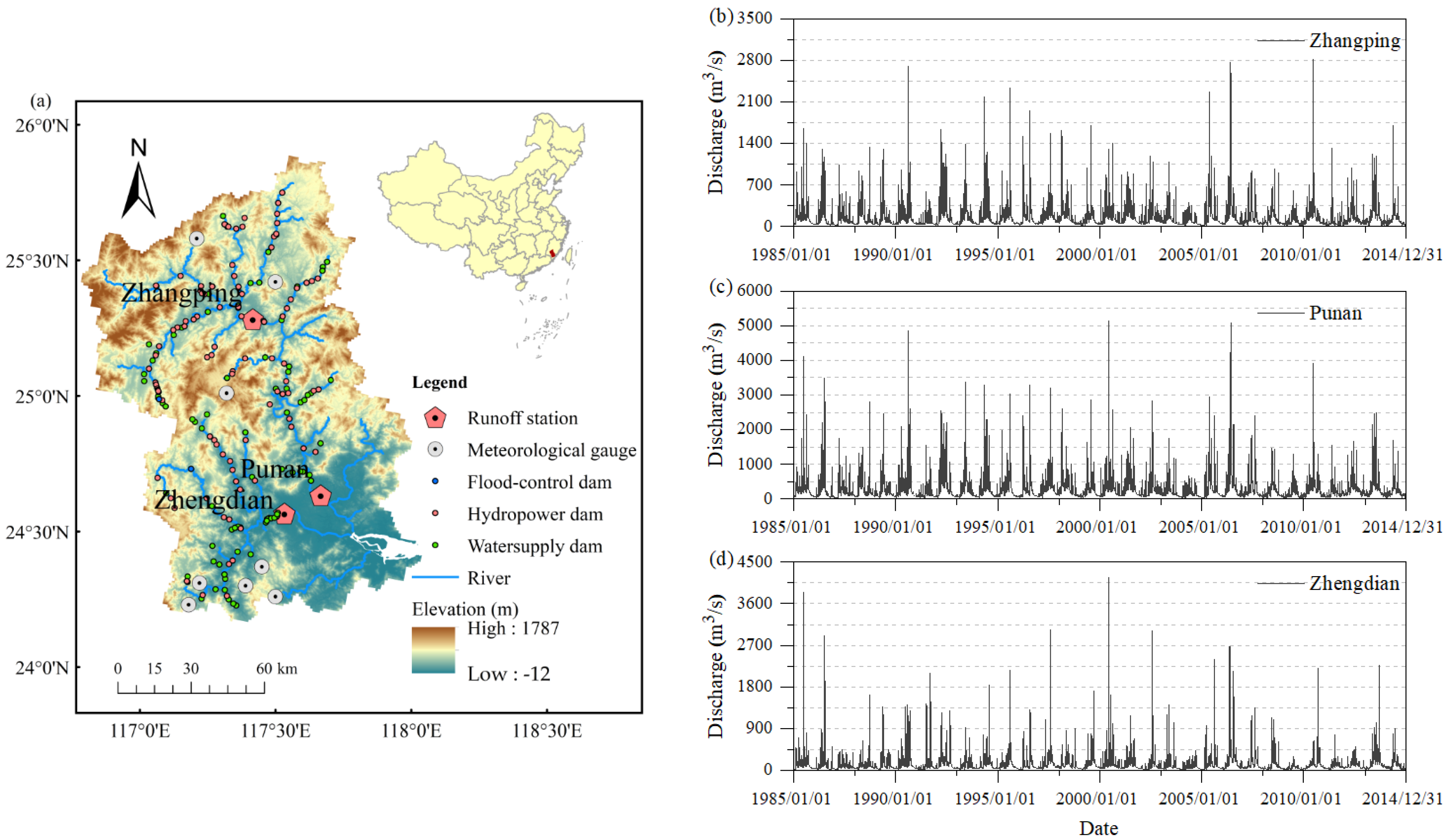
The Jiulong River basin (see Figure 1) originates in the Boping Mountains and is a coastal watershed with a drainage area of 14,741 km2. The river length is 285 km, and is the second longest river in Fujian Province, China. The basin is located in the subtropical monsoon climate zone with an average annual runoff of 1010 mm. The annual average temperature ranges from 19.9 °C to 21.1 °C, and the annual average precipitation is 1400–1800 mm, with approximately 75% of the annual precipitation occurring from April to September. The basin mainly consists of two tributaries, the North River and the West River, which cover nearly 95% of the total drainage area of the Jiulong River basin. The Jiulong River basin is profoundly impacted by dams with a total of 193 dams built in the basin by the end of 2011, and the distribution of these dams is shown in Figure 1. Among these dams, there are 2 dams built for flood control, 89 dams built for water supply and 102 dams built for hydropower. The drainage area of Zhengdian station (lower West River) has the largest capacity for flood control, while Zhangping and Punan stations (North River) have the largest capacity for hydropower.
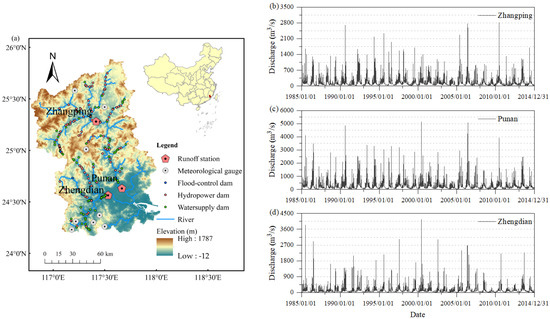
Figure 1.
Study area in the Jiulong River basin (a) and the hydrographs of hydrological stations in Zhangping (b), Punan (c) and Zhengdian (d).
2.2. Data
(1) Historical observation data
The observed meteorological data used in this study mainly contained daily air temperature (mean, maxima and minima), daily relative humidity, daily sunshine duration and daily average wind speed, which were provided by the China Meteorological Administration (CMA). The gauged meteorological data were spatially interpolated to 1-km grids by an angular distance weighting method with elevation corrections [43]. Precipitation data were obtained from the 0.25° × 0.25° China Gauge-based Daily Precipitation (CGDPA) Product [44] and were resampled to 1-km grids by nearest neighbor assignment in ArcGIS Software. Four historical land use maps in 1980, 1990, 2000 and 2010 were obtained from the Geographical Information Monitoring Cloud Platform (http://www.dsac.cn/DataProduct/Detail/20080422, accessed on 15 January 2022) at a 30-m resolution and were reclassed into 10 types: water body, urban area, bare soil, forest, irrigated cropland, upland, grassland, shrub, wetland, and ice. Daily streamflow observations at three gauges (i.e., Zhangping, Punan and Zhengdian) were obtained from the Hydrology and Water Resources Bureau. Historical LAI data were obtained from the 3rd generation of the vegetation leaf area index product (LAI3g) of the Global Inventory Modeling and Mapping Studies (GIMMS) [45]. The soil property and soil hydraulic parameter data were obtained from the China Soil Hydraulic Parameters Dataset by Duan et al. [46]. The digital elevation data were obtained from the shuttle radar topography mission (SRTM) [47] database with a resolution of 90 m.
(2) Climate outputs of GCMs and land use projections from LUH2
In this study, five newly released GCM outputs (i.e., ACCESS-ESM1-5, GFDL-ESM4, MIROC6, MPI-ESM1-2-LR and MRI-ESM2-0) under four SSP–RCP scenarios were selected from the latest CMIP6. SSP1-RCP2.6 is referred to as SSP126, SSP2-RCP4.5 is referred to as SSP245, SSP3-RCP7.0 is referred to as SSP370, and SSP5-RCP8.5 is referred to as SSP585. The GCMs selected in this study have all been applied in Asia for future climate change research in previous studies [48,49,50,51,52,53], and detailed information is shown in Table 1. The climate model outputs from 1985 to 2100 mainly contain the daily near-surface mean, maximum and minimum air temperature, daily precipitation, daily near-surface relative humidity and daily near-surface wind speed. Rooted in the socioeconomic trajectories, the newly proposed SSP–RCPs can be harmonized with the RCP previously developed in CMIP5 with shared policy assumptions and provide more plausible future scenarios [28]. The SSP1 scenario represents a green-fueled growth future; SSP2 represents a ‘middle-of-the-road’ future; SSP3 assumes high inequality between countries; and SSP5 represents a fossil-fueled growth future [54]. Future land use data were obtained from the LUH2 dataset, which provided harmonized annual land use states and transitions with a spatial resolution of 0.25° × 0.25° under four SSP–RCPs from 850 to 2100. Detailed information on LUH2 can be found in the study by Hurtt et al. [29].

Table 1.
Detailed information on GCMs selected in this study.
2.3. Methodology
2.3.1. Statistical Downscaling for Climate Outputs of GCMs
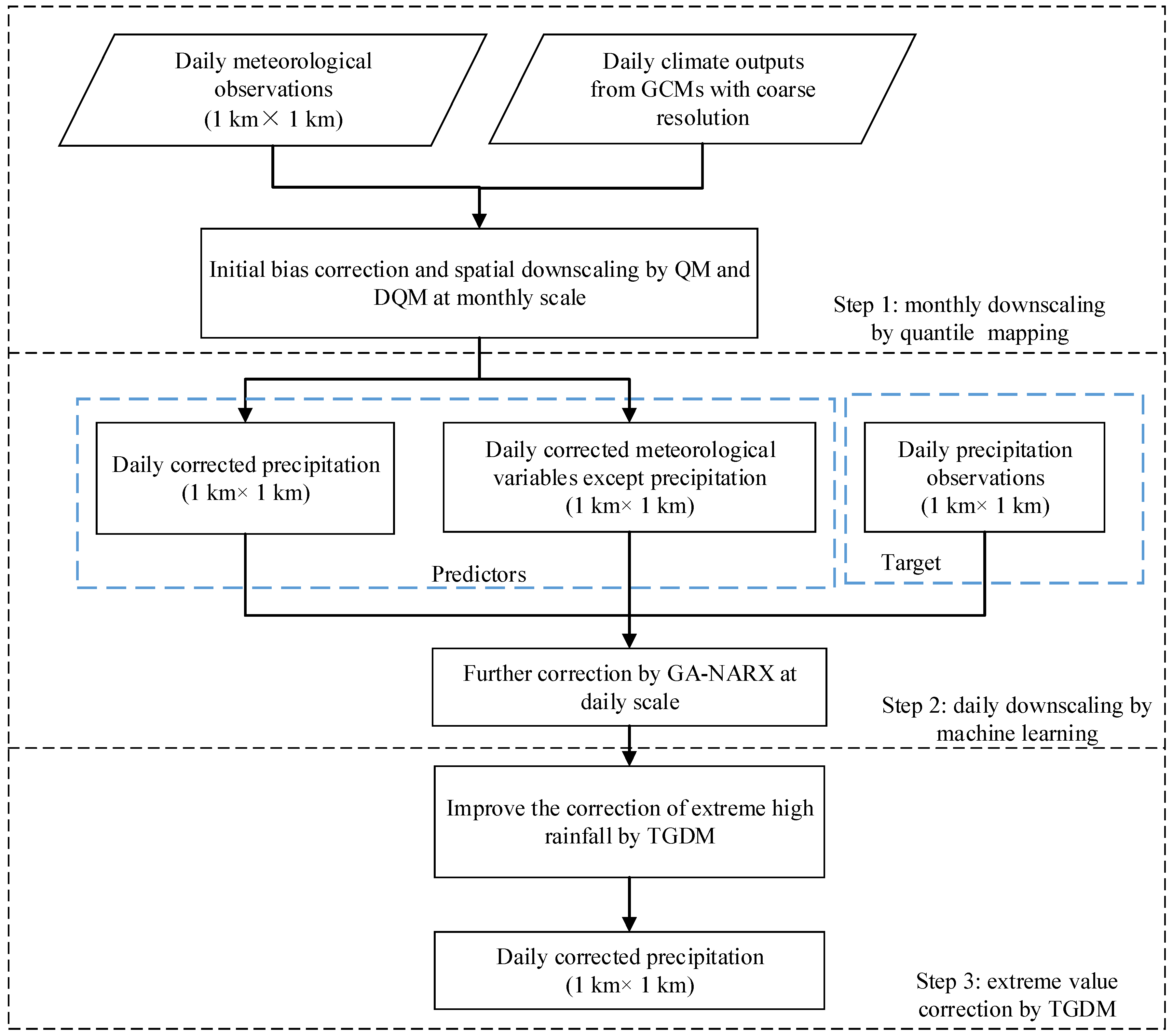
Compared with observations, the climate outputs from GCMs always contain systematic bias, and their coarse spatial resolution makes them unable to meet the high requirements of hydrological models. Therefore, it is necessary to perform bias correction and spatial downscaling on GCM outputs. In this study, we used a statistical downscaling method that combines quantile mapping (QM) and a machine learning method. The framework of this method (Figure 2) is summarized as follows:
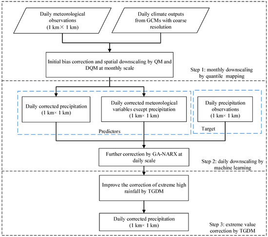
Figure 2.
Flowchart of the quantile mapping-machine learning combined method.
(1) The first step is the initial bias correction and spatial downscaling by quantile mapping (QM) [60] for the historical period and detrended quantile mapping (DQM) [61] for the future period. This step is applied to all climate variables. By matching the cumulative distribution functions (CDFs) of GCM outputs with those of observations, QM has been widely used to correct the bias between GCM outputs and observations in the field of climate change [36,38]. For bias correction in the future period, DQM removes the trend of simulations firstly and then conducts quantile mapping, eventually restoring the trend. This method can transfer the future distribution to lie within the support of the historical distribution. A detailed description of QM and DQM can be found in the studies by Piani et al. [60] and Cannon et al. [61]. Since QM or DQM mainly corrects the daily simulations on a monthly basis and the daily variability of precipitation is relatively larger, QM/DQM alone cannot meet the high requirements of daily hydrological simulation. Therefore, other methods are still needed to improve the correction at a daily scale.
(2) The second step is daily correction by machine learning. This study selected the GA-NARX [32,62] method to perform further correction for precipitation. As a class of recurrent neural networks, GA-NARX is regarded as a suitable method for nonlinear dynamic time series prediction, and a detailed description can be found in [32,62]. In this study, the predictors of GA-NARX include the QM/DQM-corrected daily rainfall, mean/maximum/minimum temperature, relative humidity and wind speed, and the target is the observed precipitation. Similar to other machine learning methods based purely on data, GA-NARX always underestimates high values [63] due to the sigmoidal activation function and insufficient training with limited high values in the time series [31,32,64]. This drawback can significantly affect the projection of future floods and needs to be overcome.
(3) The third step is extreme value correction by triple-gamma distribution mapping (TGDM). TGDM belongs to the categories of QM methods that fit CDFs by a triple-gamma distribution similar to the double-gamma distribution in Gao et al. [65] and can better capture the distribution of extremely high values. In a triple-gamma distribution, the observations and simulations are separately divided into three groups according to the specifically designed percentiles, including the 95th percentile and 99th percentile, as criteria for distinguishing normal, high and extremely high values in this study. The detailed calculation process is similar to the double-gamma distribution in Gao et al. [65] and can be found in the corresponding reference.
2.3.2. Future Land Use Projection by CA–Markov and Leaf Area Index Projection by Biome-BGC
The CA–Markov model [41] is a popular method for modeling the dynamics of spatiotemporal land use with high accuracy [66,67,68]. The Markov chain is a random process describing the transition of a system from one state to another and has the stable and memoryless property which means the probability of a random process depends only on its current state and time. A cellular automaton (CA) can independently change its state according to its previous state and that of immediate neighbors, which includes the spatial relationship in its outputs. Integrating the advantages of the Markov chain and CA, CA–Markov can reallocate land use during iterations until reaching the area totals predicted by the Markov chain. The CA–Markov model is run using IDIRISI software, and more details can be found in the IDIRISI manual [69]. In this study, we use the future land use transition area matrixes from the LUH2 dataset to replace the transition area matrixes generated by the Markov process and then run the CA–Markov model to project future high-resolution land use maps under four SSP–RCPs. The model inputs mainly include the historical land use maps (100 m × 100 m) in 2000 and 2010, and the model finally generates future 100 m × 100 m land use maps for each decade from 2020 to 2090.
The temporal and spatial dynamic distribution of vegetation is affected by both climate and land use and then constrains the hydrological process through stomatal conductance, leaf area, interception and transpiration [70,71,72,73,74]. Thus, the process of dynamic vegetation growth should be considered in hydrological simulations. As a one-dimensional process-based biogeochemical model, the Biome-BGC model [75] can robustly and accurately describe vegetation physiological processes, including photosynthesis, respiration, evapotranspiration and decomposition, in terrestrial ecosystems. The leaf area index (LAI) is estimated as a function of leaf carbon amount and is updated daily [76]. The details of Biome-BGC can be found in the studies by White et al. [77] and Thornton et al. [75]. In this study, the 4.2 version of Biome-BGC is mainly used to project future LAI with future climate forcing and land use projections under four SSP–RCPs. The eco-physiological parameters mainly include maximum stomatal conductance, fraction of leaf N in Rubisco, canopy average specific leaf area, canopy water interception coefficient, current growth proportion, year day for the start of new growth and year day for the end of litterfall, and are calibrated with remote sensing-based LAI from 1985 to 1989.
2.3.3. Hydrological Simulation by GBHM
As a fully distributed hydrological model, the geomorphology-based hydrological model (GBHM) proposed by Yang et al. [30] mainly consists of two parts: hillslope unit-based hydrological simulations and river routing along river networks. The hydrological simulation in the GBHM mainly includes canopy interception, evapotranspiration, surface flow, infiltration, unsaturated flow and groundwater flow, and river routing is based on the kinematic wave method. A detailed description of the GBHM can be found in the studies by Yang et al. [30] and Yang et al. [78]. In this study, the GBHM is used for natural hydrological simulation and projection in the Jiulong River basin with a spatial resolution of 1 km × 1 km. Since the model had been calibrated and validated with the Jiulong River basin in our previous study by Lu et al. [33], this study directly used the developed model to simulate the hydrological process during the historical period (1 January 1985–31 Decmber 2014) and the future period (1 January 2015–31 Decmber 2099). For the detailed GBHM development process in the Jiulong River basin, please refer to the previous study by Lu et al. [33].
2.3.4. Statistical Approaches for Analyzing the Changes in High and Low Flows
For the definitions of high flow and low flow, there are two common methods to describe them. One is to determine the high and low flows by the high and low percentiles based on the flow frequency distribution curve, and is widely used to validate the performance of hydrological models and can reflect the most common situations of high and low flows [32,79]. The other method of description is the annual maximum or minimum of specific moving window mean discharges, and is commonly applied to reflect flood or drought risks [27,80]. Since the changes in future hydrological hazards are focused more in this study, we selected the second method to reflect high and low flows. In this study, the high flow is reflected by annual 1-day maximum, 3-day maximum and 7-day maximum discharges calculated based on daily average discharges, and the low flow is reflected by annual 7-day minimum, 30-day minimum and 90-day minimum discharges calculated based on daily average discharges at three hydrological stations. These 6 indices we selected in this study are all contained in the indicators of hydrologic alterations (IHA) [81] to reflect the changes in flow regimes and have been widely used in previous studies [33,82,83].
To grasp the changes in future floods more accurately, the copula-based method is adopted to analyze future flood frequency. Before frequency analysis can be performed, flood events need to be identified. In this study, the peak over threshold (POT) method [84] is adopted. POT extracts flood events by setting a threshold value that leads to a specific number of flood events per year. With obvious advantages compared with the annual maximum flood series (AMF), POT can identify more flood events in wet years, ignore minor and insignificant floods in dry years, and provide more flood characteristics (such as flood volume, duration and lag time between adjacent events) [32,85]. This study adopted POT3 with three events per year, and the details of POT can be found in the studies by Lang et al. [84] and Mediero et al. [85].
Compared with classical bivariate frequency, the copula-based method performs marginal distribution and multivariate dependence modeling separately, providing greater flexibility in selecting marginal and joint probability functions [86,87]. In the field of bivariate frequency analysis, the copula function has been the dominant method and is widely used in flood frequency analysis. The copula function uses the following function to link the univariable marginal distribution functions to the multivariate probability distribution [88]:
where F1(x1), F2(x2), …, Fn(xn) are marginal distributions of the random vector (x1, x2, …, xn). A detailed description of copula functions can be found in the studies by Nelsen [89] and Salvadori et al. [90]. In this study, the flood peak and volume are selected as the marginal variables, and the candidate marginal distribution functions include the generalized extreme value (GEV), inverse Gaussian (IG), Birnbaum Saunders (BS), lognormal (LN), gamma (G), loglogistic (LL), Nakagami (Na), Rician (Ri), normal (N), logistic (L), t-location scale (T), Weibull (W), extreme value (EV), Rayleigh (Ra), exponential (Exp) and generalized Pareto (GP) distributions. The candidate copula functions include elliptical copulas (Gaussian), Archimedean copulas (Clatyon, Gumbel and Joe), extreme value copulas (Galambos), and mixture copulas (Plackett and Farlie-Gumbel-Morgenstren). All parameters were estimated using a hybrid-evolution Markov chain Monte Carlo (MCMC) approach within a Bayesian framework, and flood frequency analysis was performed by the Multivariate Copula Analysis Toolbox (MvCAT) [91,92]. A detailed mathematical description of marginal distribution functions, copula functions and joint return periods can be found in the study by Sadegh et al. [91].
3. Results
3.1. Statistical Downscaling Results of Climate Variables
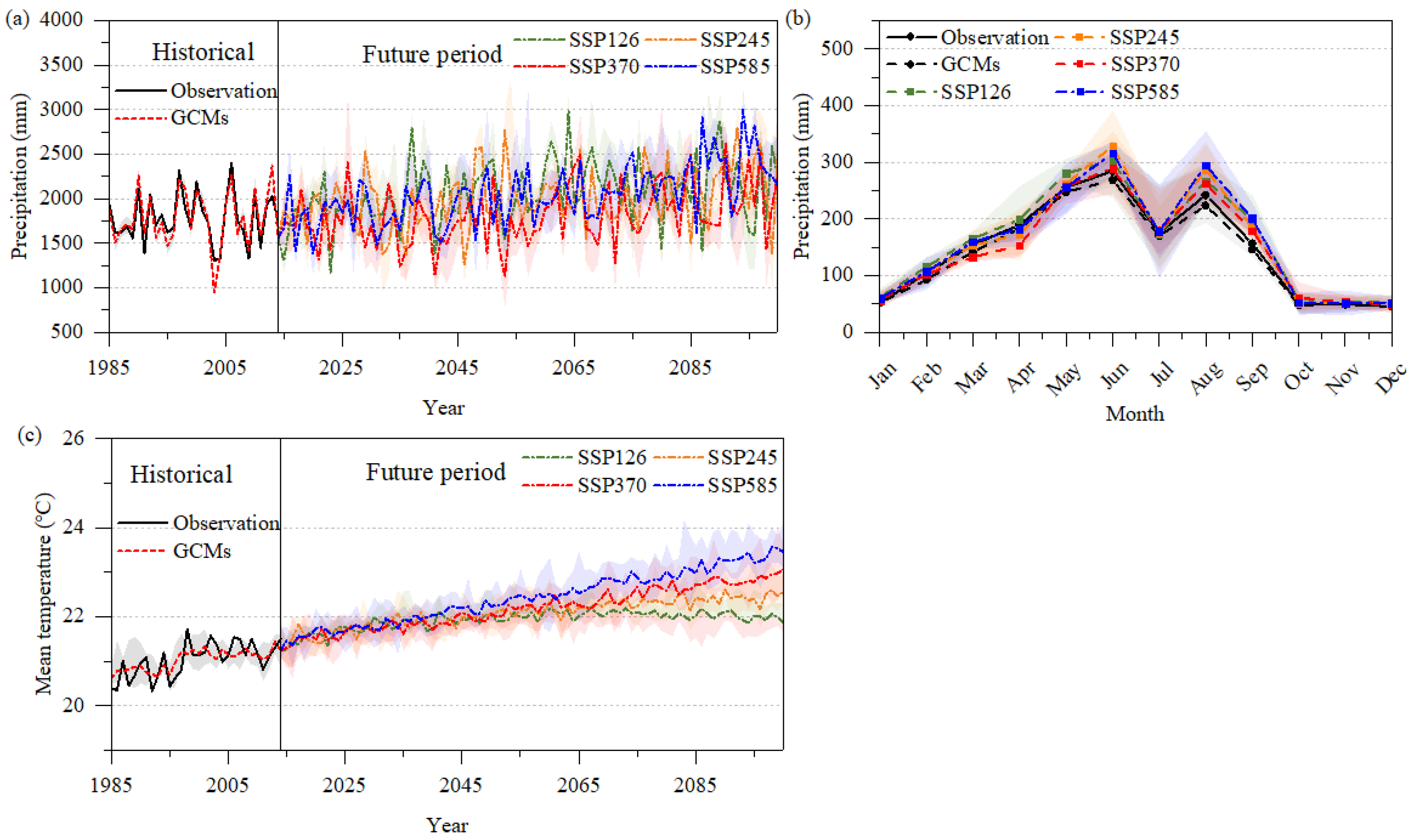
Using a combination of quantile mapping and machine learning, we performed spatial downscaling and bias correction for the coarse outputs of GCMs, and the results are shown in Figure 3. The comparison (Figure 3a) between the areal mean value of precipitation projections and observations showed that the downscaling method can satisfactorily correct the bias, and the future precipitation shows an increasing trend under the four SSP–RCPs. The fossil energy-developed SSP585 had the highest precipitation increase rate of 5.8 mm per year (0.33%/year), and the sustainably developed SSP126 had the second highest increase rate of 4.9 mm per year (0.28%/year) followed by the middle-of-the-road-developed SSP245 with an increase rate of 4.1 mm per year (0.23%/year), while the regional-rivalry-developed SSP370 had the lowest rate of increase of 2.3 mm per year (0.13%/year). In the last decade of the 21st century, annual precipitation is projected to increase by 15.5% under SSP126, 22.2% under SSP245, 14.6% under SSP370 and 24.9% under SSP585. For the inner-year temporal distribution of precipitation, the result (Figure 3b) shows that there are two peaks in a year according to the historical precipitation, which occur in June and August. In the future, two peaks still exist, with the second peak projected to increase greatly and almost surpass the first peak, which potentially indicates greater flood risks in the future. The projected annual mean temperature is shown in Figure 3c, and the results indicate that the future temperature shows different degrees of rise under the four SSP–RCPs. The sustainable development SSP126 has the slowest rise rate of 0.12 °C per decade, and continued warming will be effectively contained until 2070, subsequently showing a slight downward trend. In the last decade of the 21st century, the temperature under SSP126 will eventually increase by 0.96 ℃. The temperature under the other three SSP–RCPs will continue to rise steadily, and the rise rate will accelerate as greenhouse gas emissions increase with a rise rate of 0.16 ℃ per decade under SSP245, a rise rate of 0.19 ℃ per decade under SSP370 and 0.24 ℃ per decade under SSP585. In the last decade of the 21st century, the annual mean temperature will increase 1.42 ℃ under SSP245, 1.83 ℃ under SSP370 and 2.34 ℃ under SSP585 in the study area. In the case of constant land use, the gradual increase in temperature and precipitation in the future may increase evapotranspiration to some extent and eventually affect runoff. Since the forest coverage rate in the Jiulong River basin is nearly 57% and the evapotranspiration is largely contributed by vegetation, it is necessary to consider future land use or vegetation changes.
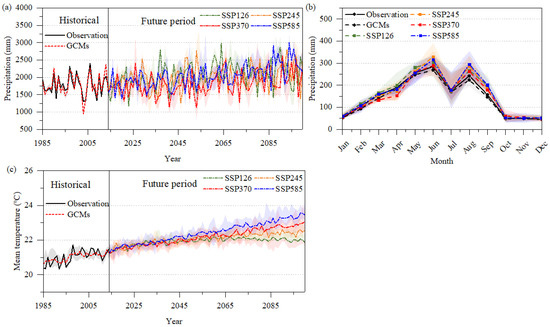
Figure 3.
The changes in annual mean precipitation (a) and air temperature (c) from the ensemble mean of corrected GCMs under the four SSP–RCPs for the period 1985–2100 and the mean monthly precipitation (b) for the period 2015–2100, while the observations (solid black line) are calculated for the period 1985–2014.
3.2. Projected Future Land Use Changes and Leaf Area Index under Various SSP–RCPs
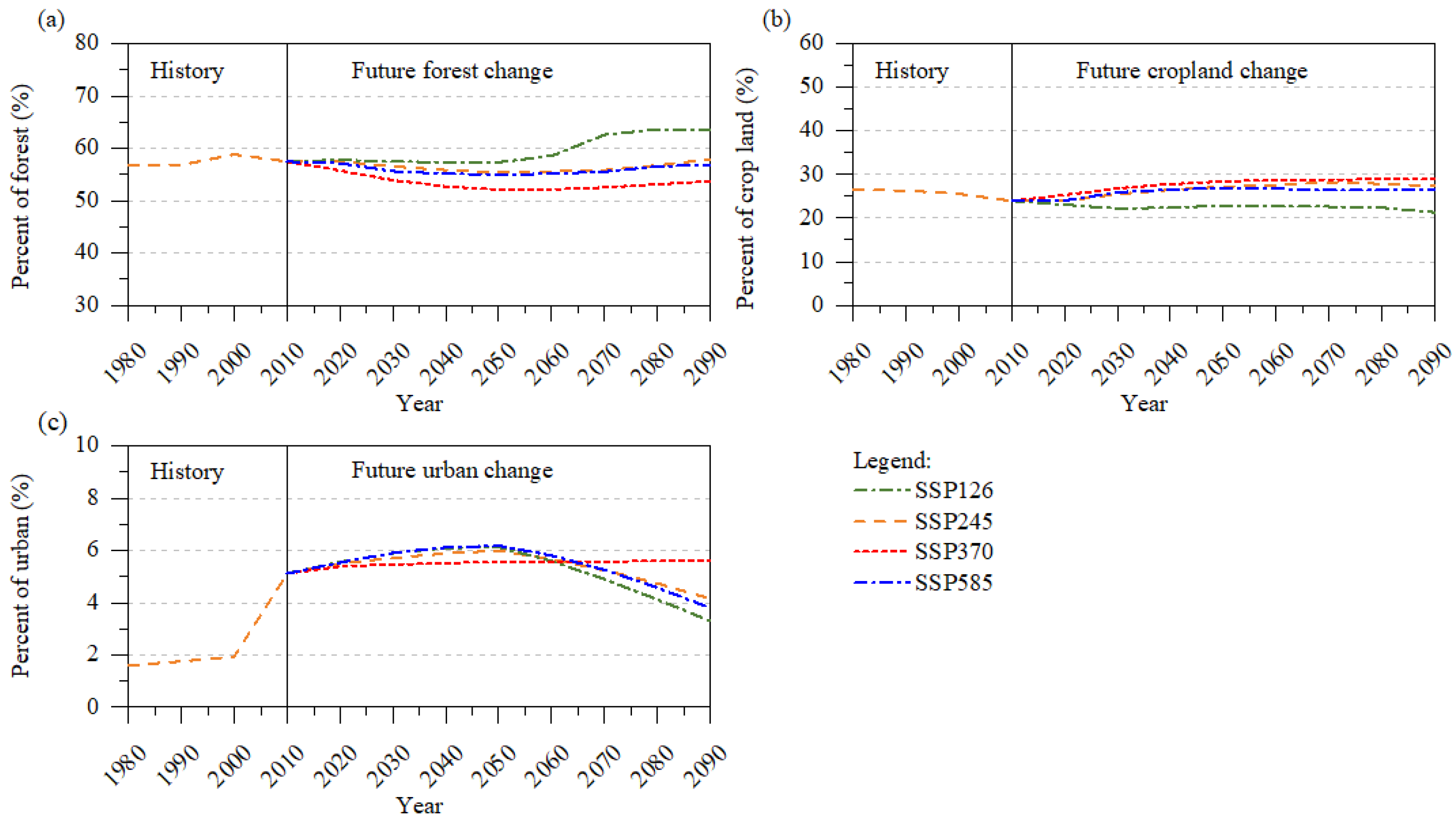
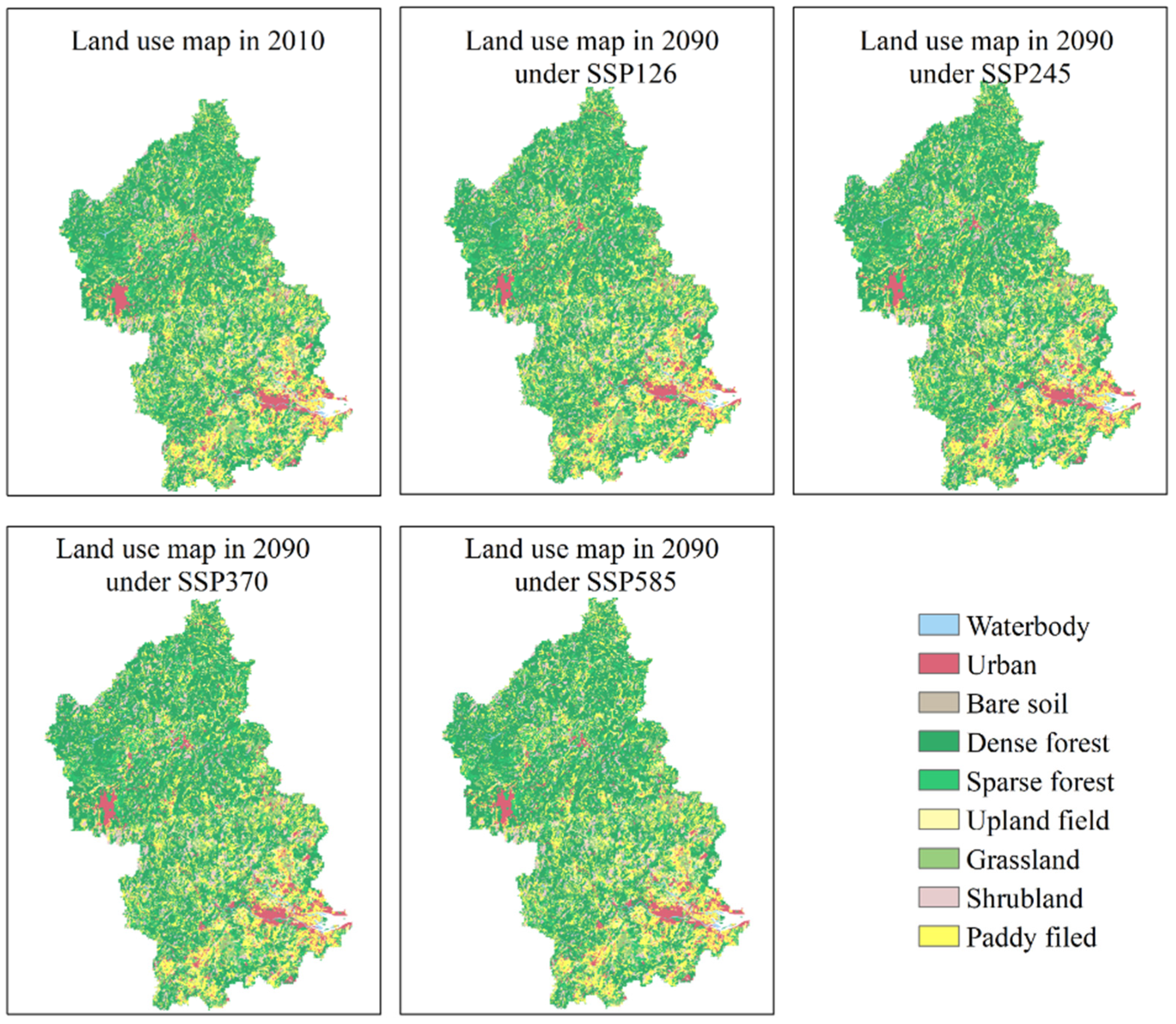
Using the CA–Markov model with land use changes from LUH2 as constraints, this study projected decadal land use maps with a spatial resolution of 100 m × 100 m from 2020 to 2090. We summarize the areal mean land use changes of forest, cropland and urban areas in Figure 4. The historical land use map in 2010 and the projected land use maps in 2090 under four scenarios are shown in Figure 5, and other projected land use maps are provided in the Supplement (see Figures S1–S4). The results show that strict land use regulations and afforestation under SSP126 will lead to a continued increase in forest growth, with the ratio of forest coverage increasing by 10.4% in 2090 compared with that in 2010 and a decreasing trend of croplands, with the ratio decreasing by 10.7% compared with that in 2010. Under the other three SSP–RCPs, the ratio of forest will initially decrease and then increase, while the ratio of croplands will initially increase and then slowly decrease. With the lack of land use regulation, SSP370 shows the greatest decrease in forest and increase in croplands in 2050. Regarding urbanization, the SSP370 scenario will essentially maintain the current urbanization rate, while other SSP–RCPs will show a declining trend after 2050.
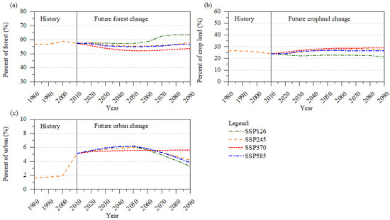
Figure 4.
The percent changes of three main land use types (forest (a), cropland (b) and urban (c) areas) with decadal land use changes projected by the CA–Markov model for the 2020-2090 period under the four SSP–RCPs. The land use changes in the historical period (1980–2010) are based on the observed land use maps.
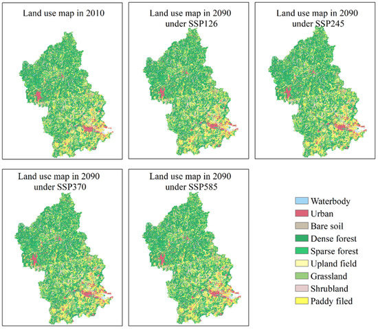
Figure 5.
The historical land use maps and the projected land use maps in 2090 under four scenarios.
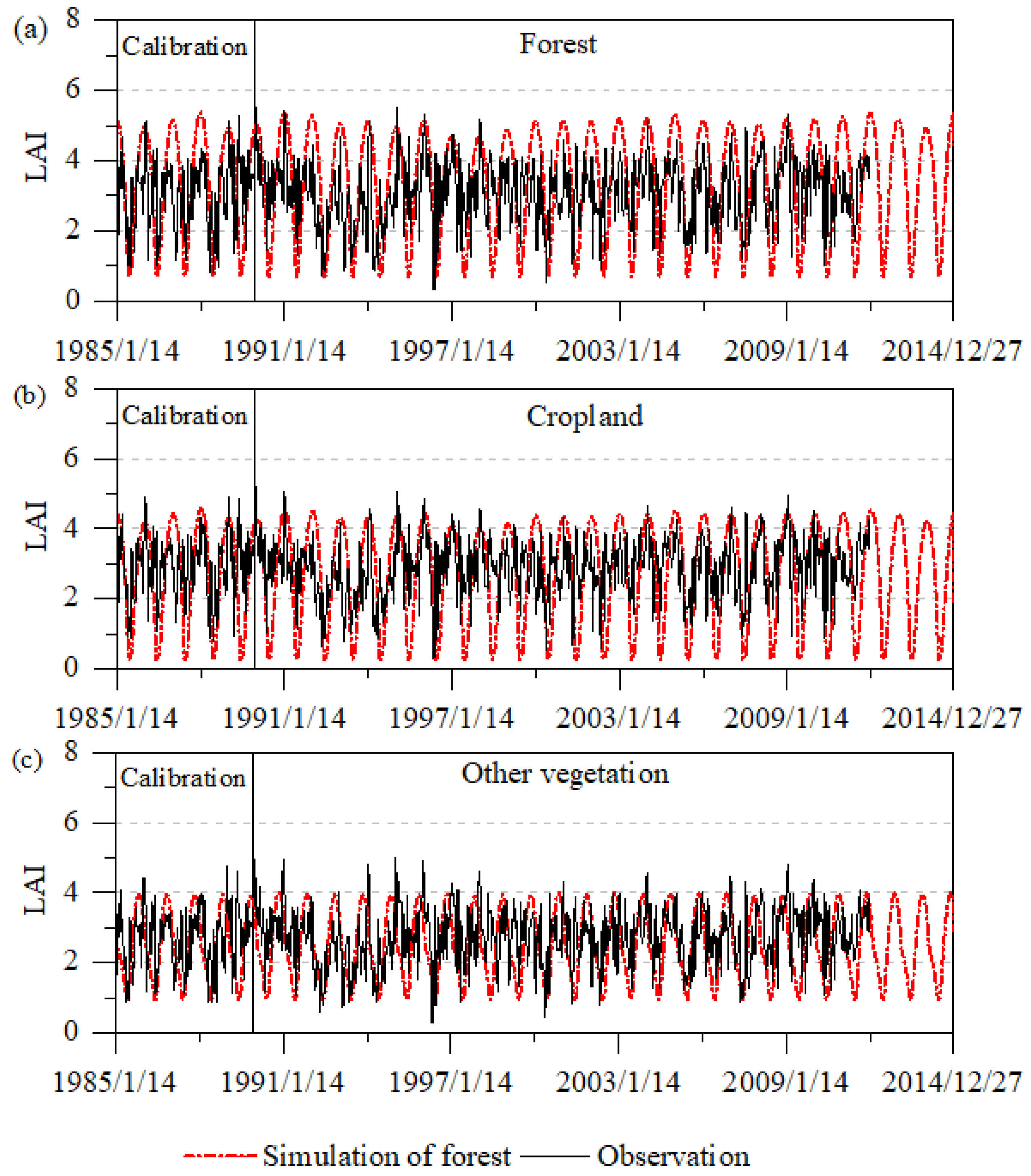
With projected land use maps and climate forcing data, the Biome-BGC model was used in this study to simulate future leaf area index (LAI) changes. First, the half-monthly remote sensing-based LAI was used to calibrate the Biome-BGC model from January 1985 to December 1989 for each type of land use and to validate the model from January 1990 to December 1994. The results (Figure 6) mainly demonstrate the model performance for the LAI simulation of forest (including dense forest and sparse forest), cropland (including paddy field and upland field) and other vegetation types (including grasses and shrubs). The calibration and validation results showed that the model can basically capture the periodic changes in LAI with correlation coefficients greater than 0.4 for each type of land use, although certain discrepancies remain between the simulation and the remote-sensing LAI, which may be caused by the lack of detailed data of some local vegetation species and we must ignore these local species. With the calibrated Biome-BGC model, the future daily LAI under the four SSP–RCPs was projected.
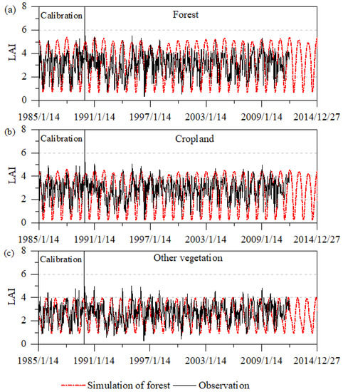
Figure 6.
The comparison between the daily simulated areal mean LAI by the Biome-BGC model and the half-monthly remote sensing-based LAI (referred to as the observation in the figure) for forest (a), cropland (b), and other vegetation (c).
3.3. Future Changes in High and Low Flows
In this study, the GBHM was used to project future hydrological processes under the four SSP–RCPs with future climate forcing, land use maps and LAI projections, and the calibration and validation of the GBHM in the Jiulong River basin can be found in our previous study by Lu et al. [33]. The previous study has proven that the GBHM can accurately reflect the natural hydrological process in the study area and the calibration and validation results are shown in Table 2. PBIAS is the percent bias between the simulation and observation and can be used to evaluate the overall model performance [93]. NSE refers to the Nash and Sutcliffe efficiency coefficient and is widely used to evaluate the performance of a hydrological model [94]. LNSE is the logarithmic-transformed Nash and Sutcliffe efficiency coefficient and is used to evaluate the capability of low flow simulation of a hydrological model [95]. A hydrological model can be regarded as a satisfactory model when PBIAS is between −10% and 10% and NSE and LNSE are greater than 0.7 according to the study by Moriasi et al. [96]. The detailed calculation equations can be found in the study by Lu et al. [33].
Table 2.
Calibration and validation results of GBHM at the Zhengdian, Zhangping and Punan stations.
The future runoff projections under the four SSP–RCPs at the three stations are shown in Table 3. The results demonstrate that future runoff is projected to show an increasing trend under all four scenarios, with the increases in runoff under SSP245 and SSP585 being relatively larger, and the lowest increase is under SSP370. At Zhengdian station, the runoff in the last decade of the 21st century is projected to increase by 29.9% under SSP126, 45.6% under SSP245, 25.3% under SSP370 and 40.0% under SSP585 compared with that in the historical period (1985–2014). At Zhangping station, the runoff in the last decade of the 21st century is projected to increase by 43.6% under SSP126, 46.0% under SSP245, 22.8% under SSP370 and 49.8% under SSP585. At Punan station, the runoff in the last decade of the 21st century is projected to increase by 41.7% under SSP126, 47.2% under SSP245, 24.5% under SSP370 and 49.3% under SSP585.
Table 3.
Annual mean runoff at the Zhengdian, Zhangping and Punan stations under the four SSP–RCPs.
3.3.1. Future Changes in High Flows
To make a preliminary assessment of future flood situations, we calculated the annual 1-day maximum, 3-day maximum and 7-day maximum discharges at three hydrological stations, with the results at the three stations shown in Figure 7. The annual 1-day maximum discharge showed the most variability, with the three stations increasing by an average of 133% under SSP126, 73% under SSP245, 68% under SSP370 and 67% under SSP585 in the last decade of the 21st century compared with that in the historical period. Annual 3-day maximum discharges had relatively less variability with the three stations increasing by an average of 141% under SSP126, 70% under SSP245, 72% under SSP370 and 64% under SSP585 in the last decade of the 21st century. The annual 7-day maximum discharges had the least variability, with the three stations increasing by an average of 144% under SSP126, 69% under SSP245, 87% under SSP370 and 64% under SSP585 in the last decade of the 21st century. The results demonstrate that the annual 1-day maximum, 3-day maximum and 7-day maximum discharges all reveal increasing trends in the future under all scenarios, which indicates that there may be more frequent floods with larger magnitudes in the future.
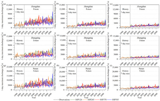
Figure 7.
Simulated annual 1-day maximum, 3-day maximum and 7-day maximum river discharges in the historical period and under the future SSP–RCPs at Zhengdian (a–c) station, Zhangping station (d–f) and Punan station (g–i).
With daily projected runoff, we used the POT3 method to extract the flood events and then used the copula-based method to simulate the bivariate joint distribution of peak-volume combinations for the historical 30-year flood, 50-year flood and 100-year flood at the three stations under the four SSP–RCPs. To display the change in flood frequency more directly, the return period was adopted. A smaller return period represents the greater likelihood a given flood is to occur with a greater exceedance frequency, and vice versa. The results shown in Table 4 indicate that the frequency of floods of different magnitudes are projected to increase under the four future scenarios. The comparison among the four SSP–RCPs shows that the future described in SSP370 and SSP585 is projected to face more frequent floods, while the situation under SSP126 is projected to encounter the lowest increase in flood frequency, with flood frequency projections under SSP245 being in the middle. At Zhengdian station, the frequency of the historical 100-year flood is projected to increase by 128% under SSP126, 128% under SSP245, 184% under SSP370, and 178% under SSP585 in the last three decades of the 21st century. At Zhangping station, the frequency of the historical 100-year flood is projected to increase by 86% under SSP126, 120% under SSP245, 239% under SSP370, and 263% under SSP585. At Punan station, the frequency of the historical 100-year flood is projected to increase by 151% under SSP126, 165% under SSP245, 215% under SSP370, and 158% under SSP585. Increasingly frequent floods in the future may cause serious damage to the lives and properties of local people in the study area, and effective mitigation and adaptation measures should be proposed to face future increasing flood risks.
Table 4.
Return periods of the historical 30-year, 50-year and 100-year floods occurring in the future at the Zhengdian, Zhangping and Punan stations under the four SSP–RCPs.
3.3.2. Future Changes in Low Flows
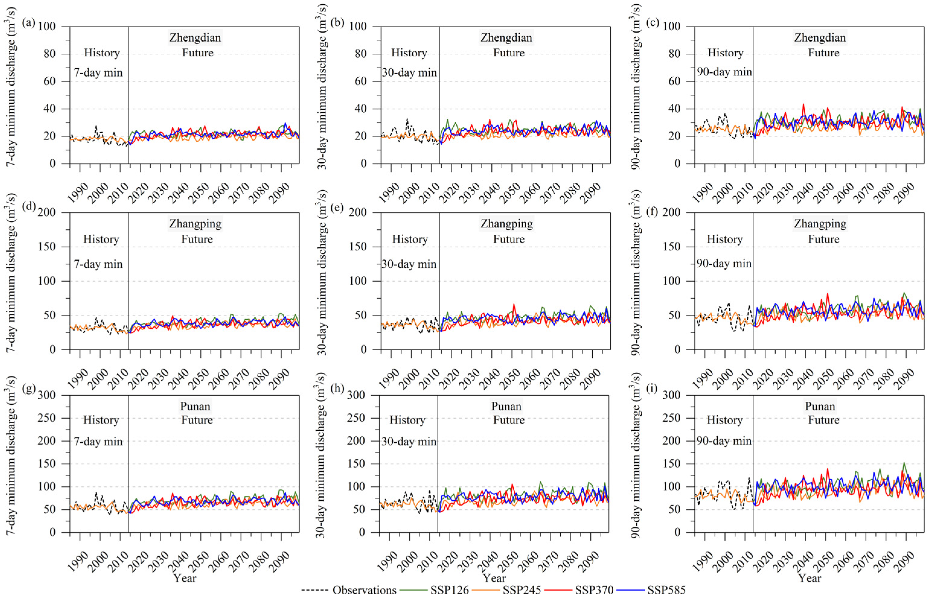
To make a preliminary assessment of future hydrological drought situations, we calculated the annual 7-day minimum, 30-day minimum and 90-day minimum discharges at three hydrological stations, and the results are shown in Figure 8. For changes in low flows, the results show that there are slightly increasing trends in the 7-day minimum, 30-day minimum and 90-day minimum discharges in the future at the three stations under the four SSP–RCPs compared with those in the historical periods. The annual 7-day minimum discharge had the least variability, with the three stations increasing by an average of 39% under SSP126, 19% under SSP245, 25% under SSP370 and 0.26% under SSP585 in the last decade of the 21st century compared to that in the historical period. Annual 30-day minimum discharges have relatively greater variability with the three stations increasing by an average of 41% under SSP126, 18% under SSP245, 24% under SSP370, and 31% under SSP585 in the last decade of the 21st century. The annual 90-day minimum discharges had the most variability, with the three stations increasing by an average of 36% under SSP126, 13% under SSP245, 25% under SSP370, and 29% under SSP585 in the last decade of the 21st century. This indicates that future hydrological droughts may be alleviated to some extent, although droughts have not been a severe problem in the Jiulong River basin.
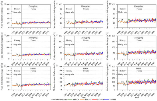
Figure 8.
Simulated annual 7-day minimum, 30-day minimum and 90-day minimum river discharges in the historical period and under the future SSP–RCPs at Zhengdian (a–c) station, Zhangping station (d–f) and Punan station (g–i).
4. Discussion
4.1. Impact of Climate and Land Use Changes on Future High and Low Flows
The above results have demonstrated a wetter and warmer future in this coastal basin and analyzed potential changes in future runoff and flood frequency under the combined impacts of climate change and land use change. However, the respective impacts of climate change and land use change need to be further discussed. Here, we replaced the historical 30-year climate forcing data with the projected 30-year (2071–2100) future climate data under SSP370 and retained the historical land use (referred to as the newly designed scenario). The LAI was simulated by the calibrated Biome-BGC model, and the hydrological process was projected using the calibrated GBHM model. Since SSP370 and the newly designed scenario had the same precipitation in 2071–2100 with the only difference being in land use change, the comparison between these two scenarios could show the impact of land use change. Similarly, the only difference observed between the historical situation and the newly designed scenario was the change of climate forcing data, and the comparison between these two scenarios could quantify the impact of climate change. The annual 1-day maximum discharge was selected to represent high flow, and the annual 7-day minimum discharge was chosen to represent low flow.
For high flow, the comparison results showed that the mean value of annual 1-day maximum discharge under the newly designed scenario is projected to increase by 106% at Zhengdian station, 100% at Zhangping station and 48% at Punan station compared to that in the historical period (1985–2014), while that under SSP370 is projected to increase by 128% at Zhengdian station, 103% at Zhangping station and 51% at Punan station. It can be concluded that climate change is a dominating factor for the future increase in high flows with larger precipitation during the wet season. The comparison between the newly designed scenario and SSP370 shows that continuous deforestation and cropland extension under SSP370 will exacerbate this increase (from 106% to 128% at Zhengdian station, 100% to 103% at Zhangping station and 48% to 51% at Punan station) by affecting canopy interception, infiltration and evapotranspiration processes, which is consistent with previous studies [97,98,99]. For low flow, the results demonstrate that the mean value of annual 7-day minimum discharge under the newly designed scenario will increase by 8.5% at Zhengdian station, 8.4% at Zhangping station and 9.5% at Punan station, while that under SSP370 will increase by 27.2% at Zhengdian station, 31.3% at Zhangping station and 19.3% at Punan station. This indicates that future climate change in the Jiulong River basin may have less impact on low flows, while land use changes (deforestation and cropland extension) will cause an increase in low flows. The main reason for this phenomenon is that forest degradation reduces evapotranspiration and canopy interception, which leads to an increase in soil water content and groundwater recharge and ultimately causes an increase in low flow [1,100].
4.2. Impact of Dams on Futrue High and Low Flows
Since there are numerous dams existing in the Jiulong River basin, the possible impacts of dams on future high and low flows are desired points of discussion. However, since the GBHM model we used in this study did not have the reservoir operation module which requires further improvement, it was difficult to quantitatively analyze the current impact of dams thus we only quantitatively discussed the possible impacts here. The drainage area of Zhengdian station is mainly affected by annual flood-control dams according to the reservoir capacities, and the drainage area of Zhangping and Punan stations are mainly affected by small-scale hydropower dams (<50 MW). Our previous study [33] showed that the flood-control dams could decrease the high flows and increase the low flows at Zhengdian station by releasing water in dry seasons and restraining floods in wet seasons, while at Zhangping and Punan stations, the dominant hydropower dams could reduce low flows and had less obvious effects on high flows. This is due to these small dams being built solely to generate as much electricity as possible and may thus store more water up to a sufficient head before electricity generation can occur during the dry season. Under a future with increasing high flows and frequent floods, the flood-control dams may to some extent mitigate the growth of high flows and reduce flood risks in addition to increasing low flows at Zhengdian station. However, the numerous small-scale hydropower dams may have less effect on the reduction of high flows and mitigation of flood risks at Zhangping and Punan stations, and the slight increase in low flows due to climate and land use changes may be offset to some extent by the reduction effect from hydropower dams, thus low flows at these two stations may not change much in the future.
4.3. Suggestions for Future Water Management
According to the results found in this study, the Jiulong River basin faces a challenging future with more frequent floods, and a wetter and warmer climate will dominate the increase in high flows, which will be further exacerbated by forest degradation. Current water management systems will be severely challenged and need to be adjusted. Integrated water management is required in the future. First, as regional positive and sustainable land use changes can offset the impacts of climate change to some extent, we suggest that local authorities implement strict land management practices and vigorously promote afforestation. Second, we recommend that the flood protection standards of the infrastructure should be improved in the Jiulong River basin, which is in close proximity to several cities with large populations and thriving economies. Third, we suggest that the management department should improve the operation rules of numerous existing reservoirs to adapt to more severe flood situations in the future.
5. Conclusions
With a combined downscaling quantile mapping-machine learning method, the future climate forcing data from GCMs in CMIP6 were bias corrected and spatially downscaled. Using the CA–Markov model with future land use changes from LUH2 as constraints, decadal future land use maps with high spatial resolution were projected. Based on the climate forcing and land use projections, the Biome-BGC model was applied to project future LAI data, and subsequently, a calibrated hydrological model (GBHM) was used to simulate the future hydrological process under four SSP–RCPs during the period from 2015 to 2100. The main conclusions were as follows:
(1) Under global warming, precipitation and air temperature will continue to rise under all SSP–RCPs. In the last decade of the 21st century, precipitation is projected to increase by 15.5% under SSP126, 22.2% under SSP245, 14.6% under SSP370 and 24.9% under SSP585, and the annual mean temperature will increase by 0.96 ℃ under SSP126, 1.42 ℃ under SSP245, 1.83 ℃ under SSP370 and 2.34 ℃ under SSP585 in the study area.
(2) In the future, land use changes will have different development pathways determined by the initial designs in various SSP–RCPs. Under greenest roads (SSP126), the forest area will continue to rise with the ratio increasing by 10.4% in 2090, and the cropland decreasing by 10.7% compared with that in 2010. Under the other three SSP–RCPs, the ratio of forest will initially decrease and then increase, while the ratio of croplands will initially increase and then slowly decrease.
(3) Under the combined impacts of climate and land use change, the total available water resources will increase due to increasing precipitation, and the high flow and low flow will both increase at three stations under the four SSP–RCPs. In addition, the Jiulong River basin will face more frequent floods in the future. In the last three decades of the 21st century, the station-average frequency of a historical 100-year flood will increase by 122% under the most optimistic of scenarios (SSP126), and increase by 213% under the scenario of greatest regional rivalry (SSP370).
(4) Future warmer and wetter climates will lead to a great increase in high flows, and deforestation will exacerbate this increase to some extent, while the increase in low flows mainly caused by land use changes (deforestation and cropland extension), and the impact of climate change will be relatively smaller.
(5) To tackle the challenges of future water management presented by climate change, we recommend an integrated water management system, including afforestation, raised protection standards of infrastructure and improvement of existing operation rules of numerous reservoirs.
Supplementary Materials
The following supporting information can be downloaded at: https://www.mdpi.com/article/10.3390/atmos13020150/s1, Figure S1: The projected land use maps under SSP126; Figure S2: The projected land use maps under SSP245; Figure S3: The projected land use maps under SSP370; Figure S4: The projected land use maps under SSP585.
Author Contributions
Conceptualization, S.Y. and D.Y.; Data curation, S.Y.; Formal analysis, S.Y.; Funding acquisition, D.Y. and J.S.; Investigation, S.Y.; Methodology, S.Y.; Project administration, D.Y.; Resources, W.L.; Software, S.Y.; Supervision, D.Y.; Writing—original draft, S.Y.; Writing—review & editing, S.Y., B.Z. and T.M. All authors have read and agreed to the published version of the manuscript.
Funding
This research was funded by the National Natural Science Foundation of China (Grant No. 41661144031).
Institutional Review Board Statement
Not applicable.
Informed Consent Statement
Not applicable.
Data Availability Statement
GIMMS LAI3g is available at https://ecocast.arc.nasa.gov/data/pub/gimms/3g.v1/, accessed on 15 January 2022. The GCM data can be directly downloaded at https://esgf-node.llnl.gov/search/cmip6/, accessed on 15 January 2022. The LUH2 dataset is available at https://luh.umd.edu/data.shtml, accessed on 15 January 2022. The other datasets analyzed during the current study are available from the corresponding author upon reasonable request.
Acknowledgments
The authors are grateful to the anonymous reviewers for their invaluable comments and for editing a previous draft of the manuscript. The authors are appreciative of the datasets used in this study provided by the researchers and their teams.
Conflicts of Interest
The authors declare no conflict of interest.
References
- Yang, W.; Long, D.; Bai, P. Impacts of future land cover and climate changes on runoff in the mostly afforested river basin in North China. J. Hydrol. 2019, 570, 201–219. [Google Scholar] [CrossRef]
- Wang, Y.; Wang, A.; Zhai, J.; Tao, H.; Jiang, T.; Su, B.; Yang, J.; Wang, G.; Liu, Q.; Gao, C.; et al. Tens of thousands additional deaths annually in cities of China between 1.5 degrees C and 2.0 degrees C warming. Nat. Commun. 2019, 10, 3376. [Google Scholar] [CrossRef] [PubMed]
- Russo, S.; Dosio, A.; Graversen, R.G.; Sillmann, J.; Carrao, H.; Dunbar, M.B.; Singleton, A.; Montagna, P.; Barbola, P.; Vogt, J.V. Magnitude of extreme heat waves in present climate and their projection in a warming world. J. Geophys. Res. Atmos. 2014, 119, 12500–12512. [Google Scholar] [CrossRef] [Green Version]
- Trenberth, K.E.; Dai, A.; van der Schrier, G.; Jones, P.D.; Barichivich, J.; Briffa, K.R.; Sheffield, J. Global warming and changes in drought. Nat. Clim. Change 2013, 4, 17–22. [Google Scholar] [CrossRef]
- Donat, M.G.; Lowry, A.L.; Alexander, L.V.; O’Gorman, P.A.; Maher, N. More extreme precipitation in the world’s dry and wet regions. Nat. Clim. Change 2016, 6, 508–513. [Google Scholar] [CrossRef]
- Bellard, C.; Bertelsmeier, C.; Leadley, P.; Thuiller, W.; Courchamp, F. Impacts of climate change on the future of biodiversity. Ecol. Lett. 2012, 15, 365–377. [Google Scholar] [CrossRef] [PubMed] [Green Version]
- Wang, X.; Zhao, C.; Müller, C.; Wang, C.; Ciais, P.; Janssens, I.; Peñuelas, J.; Asseng, S.; Li, T.; Elliott, J.; et al. Emergent constraint on crop yield response to warmer temperature from field experiments. Nat. Sustain. 2020, 3, 908–916. [Google Scholar] [CrossRef]
- Zhang, W.; Zhou, T.; Zou, L.; Zhang, L.; Chen, X. Reduced exposure to extreme precipitation from 0.5 degrees C less warming in global land monsoon regions. Nat. Commun. 2018, 9, 3153. [Google Scholar] [CrossRef] [Green Version]
- Bermúdez, M.; Farfán, J.F.; Willems, P.; Cea, L. Assessing the Effects of Climate Change on Compound Flooding in Coastal River Areas. Water Resour. Res. 2021, 57, e2020WR029321. [Google Scholar] [CrossRef]
- Koks, E.E.; Jongman, B.; Husby, T.G.; Botzen, W.J.W. Combining hazard, exposure and social vulnerability to provide lessons for flood risk management. Environ. Sci. Policy 2015, 47, 42–52. [Google Scholar] [CrossRef]
- Pratoomchai, W.; Kazama, S.; Ekkawatpanit, C.; Komori, D. Opportunities and constraints in adapting to flood and drought conditions in the Upper Chao Phraya River basin in Thailand. Int. J. River Basin Manag. 2015, 13, 413–427. [Google Scholar] [CrossRef]
- Alfieri, L.; Bisselink, B.; Dottori, F.; Naumann, G.; de Roo, A.; Salamon, P.; Wyser, K.; Feyen, L. Global projections of river flood risk in a warmer world. Earth’s Future 2017, 5, 171–182. [Google Scholar] [CrossRef]
- Bates, P.D.; Quinn, N.; Sampson, C.; Smith, A.; Wing, O.; Sosa, J.; Savage, J.; Olcese, G.; Neal, J.; Schumann, G.; et al. Combined Modeling of US Fluvial, Pluvial, and Coastal Flood Hazard Under Current and Future Climates. Water Resour. Res. 2021, 57, e2020WR028673. [Google Scholar] [CrossRef]
- Hirabayashi, Y.; Mahendran, R.; Koirala, S.; Konoshima, L.; Yamazaki, D.; Watanabe, S.; Kim, H.; Kanae, S. Global flood risk under climate change. Nat. Clim. Change 2013, 3, 816–821. [Google Scholar] [CrossRef]
- Liu, W.; Yang, T.; Sun, F.; Wang, H.; Feng, Y.; Du, M. Observation-Constrained Projection of Global Flood Magnitudes With Anthropogenic Warming. Water Resour. Res. 2021, 57, e2020WR028830. [Google Scholar] [CrossRef]
- Ma, Q.; Xiong, L.; Xu, C.-Y.; Li, R.; Ji, C.; Zhang, Y. Flood Wave Superposition Analysis Using Quantitative Matching Patterns of Peak Magnitude and Timing in Response to Climate Change. Water Resour. Manag. 2021, 35, 2409–2432. [Google Scholar] [CrossRef]
- Alfieri, L.; Burek, P.; Feyen, L.; Forzieri, G. Global warming increases the frequency of river floods in Europe. Hydrol. Earth Syst. Sci. 2015, 19, 2247–2260. [Google Scholar] [CrossRef] [Green Version]
- Rottler, E.; Bronstert, A.; Bürger, G.; Rakovec, O. Projected changes in Rhine River flood seasonality under global warming. Hydrol. Earth Syst. Sci. 2021, 25, 2353–2371. [Google Scholar] [CrossRef]
- Arnell, N.W. Relative effects of multi-decadal climatic variability and changes in the mean and variability of climate due to global warming: Future streamflows in Britain. J. Hydrol. 2003, 270, 195–213. [Google Scholar] [CrossRef]
- Bai, P.; Liu, X.; Zhang, Y.; Liu, C. Assessing the Impacts of Vegetation Greenness Change on Evapotranspiration and Water Yield in China. Water Resour. Res. 2020, 56, e2019WR027019. [Google Scholar] [CrossRef]
- Baker, T.J.; Miller, S.N. Using the Soil and Water Assessment Tool (SWAT) to assess land use impact on water resources in an East African watershed. J. Hydrol. 2013, 486, 100–111. [Google Scholar] [CrossRef]
- Li, C.; Sun, G.; Caldwell, P.V.; Cohen, E.; Fang, Y.; Zhang, Y.; Oudin, L.; Sanchez, G.M.; Meentemeyer, R.K. Impacts of Urbanization on Watershed Water Balances Across the Conterminous United States. Water Resour. Res. 2020, 56, e2019WR026574. [Google Scholar] [CrossRef]
- Aich, V.; Liersch, S.; Vetter, T.; Fournet, S.; Andersson, J.C.M.; Calmanti, S.; van Weert, F.H.A.; Hattermann, F.F.; Paton, E.N. Flood projections within the Niger River Basin under future land use and climate change. Sci. Total Environ. 2016, 562, 666–677. [Google Scholar] [CrossRef]
- Chacuttrikul, P.; Kiguchi, M.; Oki, T. Impacts of climate and land use changes on river discharge in a small watershed: A case study of the Lam Chi subwatershed, northeast Thailand. Hydrol. Res. Lett. 2018, 12, 7–13. [Google Scholar] [CrossRef]
- Pervez, M.S.; Henebry, G.M. Assessing the impacts of climate and land use and land cover change on the freshwater availability in the Brahmaputra River basin. J. Hydrol. Reg. Stud. 2015, 3, 285–311. [Google Scholar] [CrossRef] [Green Version]
- Wang, S.; Kang, S.; Zhang, L.; Li, F. Modelling hydrological response to different land-use and climate change scenarios in the Zamu River basin of northwest China. Hydrol. Processes 2008, 22, 2502–2510. [Google Scholar] [CrossRef]
- Tavakoli, M.; De Smedt, F.; Vansteenkiste, T.; Willems, P. Impact of climate change and urban development on extreme flows in the Grote Nete watershed, Belgium. Nat. Hazards 2014, 71, 2127–2142. [Google Scholar] [CrossRef]
- NCC, E. The CMIP6 landscape. Nat. Clim. Change 2019, 9, 727. [Google Scholar] [CrossRef] [Green Version]
- Hurtt, G.C.; Chini, L.; Sahajpal, R.; Frolking, S.; Bodirsky, B.L.; Calvin, K.; Doelman, J.C.; Fisk, J.; Fujimori, S.; Goldewijk, K.K.; et al. Harmonization of Global Land-Use Change and Management for the Period 850-2100 (LUH2) for CMIP6. Geosci. Model Dev. 2020, 2020, 1–65. [Google Scholar] [CrossRef]
- Yang, D.; Herath, S.; Musiake, K. Development of a geomorphology-based hydrological model for large catchments. Proc. Hydraul. Eng. 1998, 42, 169–174. [Google Scholar] [CrossRef] [Green Version]
- Yang, S.; Yang, D.; Chen, J.; Santisirisomboon, J.; Lu, W.; Zhao, B. A physical process and machine learning combined hydrological model for daily streamflow simulations of large watersheds with limited observation data. J. Hydrol. 2020, 590, 125206. [Google Scholar] [CrossRef]
- Yang, S.; Yang, D.; Chen, J.; Zhao, B. Real-time reservoir operation using recurrent neural networks and inflow forecast from a distributed hydrological model. J. Hydrol. 2019, 579, 124229. [Google Scholar] [CrossRef]
- Lu, W.; Lei, H.; Yang, D.; Tang, L.; Miao, Q. Quantifying the impacts of small dam construction on hydrological alterations in the Jiulong River basin of Southeast China. J. Hydrol. 2018, 567, 382–392. [Google Scholar] [CrossRef]
- Wang, W.; Lu, H.; Yang, D.; Sothea, K.; Jiao, Y.; Gao, B.; Peng, X.; Pang, Z. Modelling hydrologic processes in the Mekong River Basin using a distributed model driven by satellite precipitation and rain gauge observations. PLoS ONE 2016, 11, e0152229. [Google Scholar] [CrossRef] [PubMed] [Green Version]
- Li, Z.; Yang, D.; Gao, B.; Jiao, Y.; Hong, Y.; Xu, T. Multi-scale hydrologic applications of the latest satellite precipitation products in the Yangtze River basin using a distributed hydrological model. J. Hydrometeorol. 2015, 16, 407–426. [Google Scholar] [CrossRef]
- Chen, J.; Brissette, F.P.; Chaumont, D.; Braun, M. Performance and uncertainty evaluation of empirical downscaling methods in quantifying the climate change impacts on hydrology over two North American river basins. J. Hydrol. 2013, 479, 200–214. [Google Scholar] [CrossRef]
- Mamalakis, A.; Langousis, A.; Deidda, R.; Marrocu, M. A parametric approach for simultaneous bias correction and high-resolution downscaling of climate model rainfall. Water Resour. Res. 2017, 53, 2149–2170. [Google Scholar] [CrossRef]
- Guo, Q.; Chen, J.; Zhang, X.J.; Xu, C.Y.; Chen, H. Impacts of Using State-of-the-Art Multivariate Bias Correction Methods on Hydrological Modeling Over North America. Water Resour. Res. 2020, 56. [Google Scholar] [CrossRef]
- Kamusoko, C.; Aniya, M.; Adi, B.; Manjoro, M. Rural sustainability under threat in Zimbabwe–Simulation of future land use/cover changes in the Bindura district based on the Markov-cellular automata model. Appl. Geogr. 2009, 29, 435–447. [Google Scholar] [CrossRef]
- Lambin, E.F.; Rounsevell, M.D.A.; Geist, H.J. Are agricultural land-use models able to predict changes in land-use intensity? Agric. Ecosyst. Environ. 2000, 82, 321–331. [Google Scholar] [CrossRef]
- Du, J.; Qian, L.; Rui, H.; Zuo, T.; Zheng, D.; Xu, Y.; Xu, C.Y. Assessing the effects of urbanization on annual runoff and flood events using an integrated hydrological modeling system for Qinhuai River basin, China. J. Hydrol. 2012, 464–465, 127–139. [Google Scholar] [CrossRef]
- Fu, X.; Wang, X.; Yang, Y.J. Deriving suitability factors for CA-Markov land use simulation model based on local historical data. J. Environ. Manag. 2018, 206, 10–19. [Google Scholar] [CrossRef] [PubMed]
- Yang, D.; Li, C.; Hu, H.; Lei, Z.; Yang, S.; Kusuda, T.; Koike, T.; Musiake, K. Analysis of water resources variability in the Yellow River of China during the last half century using historical data. Water Resour. Res. 2004, 40, 308–322. [Google Scholar] [CrossRef]
- Shen, Y.; Zhao, P.; Pan, Y.; Yu, J. A high spatiotemporal gauge-satellite merged precipitation analysis over China. J. Geophys. Res. Atmos. 2014, 119, 3063–3075. [Google Scholar] [CrossRef]
- Zhu, Z.; Bi, J.; Pan, Y.; Ganguly, S.; Anav, A.; Xu, L.; Samanta, A.; Piao, S.; Nemani, R.; Myneni, R. Global Data Sets of Vegetation Leaf Area Index (LAI)3g and Fraction of Photosynthetically Active Radiation (FPAR)3g Derived from Global Inventory Modeling and Mapping Studies (GIMMS) Normalized Difference Vegetation Index (NDVI3g) for the Period 1981 to 2011. Remote Sens. 2013, 5, 927–948. [Google Scholar] [CrossRef] [Green Version]
- Duan, Q.; Shangguan, W.; Dai, Y.; Liu, B.; Fu, S.; Niu, G. Development of a China Dataset of Soil Hydraulic Parameters Using Pedotransfer Functions for Land Surface Modeling. J. Hydrometeorol. 2013, 14, 869–887. [Google Scholar] [CrossRef] [Green Version]
- Jarvis, A.; Reuter, H.I.; Nelson, A.; Guevara, E. Hole-Filled Seamless SRTMdata V4, International Centre for Tropical Agriculture (CIAT). 2008. Available online: https://cgiarcsi.community/data/srtm-90m-digital-elevation-database-v4-1/ (accessed on 15 January 2022).
- Okwala, T.; Shrestha, S.; Ghimire, S.; Mohanasundaram, S.; Datta, A. Assessment of climate change impacts on water balance and hydrological extremes in Bang Pakong-Prachin Buri river basin, Thailand. Environ. Res. 2020, 186, 109544. [Google Scholar] [CrossRef]
- Panjwani, S.; Naresh Kumar, S.; Ahuja, L.; Islam, A. Prioritization of global climate models using fuzzy analytic hierarchy process and reliability index. Theor. Appl. Climatol. 2019, 137, 2381–2392. [Google Scholar] [CrossRef]
- Preethi, B.; Mujumdar, M.; Prabhu, A.; Kripalani, R. Variability and teleconnections of South and East Asian summer monsoons in present and future projections of CMIP5 climate models. Asia-Pac. J. Atmos. Sci. 2017, 53, 305–325. [Google Scholar] [CrossRef]
- Plangoen, P.; Udmale, P. Impacts of Climate Change on Rainfall Erosivity in the Huai Luang Watershed, Thailand. Atmosphere 2017, 8, 143. [Google Scholar] [CrossRef] [Green Version]
- Hunukumbura, P.B.; Tachikawa, Y. River Discharge Projection under Climate Change in the Chao Phraya River Basin, Thailand, Using the MRI-GCM3.1S Dataset. J. Meteorol. Soc. Jpn. 2012, 90A, 137–150. [Google Scholar] [CrossRef] [Green Version]
- Singhrattna, N.; Singh Babel, M. Changes in summer monsoon rainfall in the Upper Chao Phraya River Basin, Thailand. Clim. Res. 2011, 49, 155–168. [Google Scholar] [CrossRef] [Green Version]
- Gidden, M.J.; Riahi, K.; Smith, S.J.; Fujimori, S.; Luderer, G.; Kriegler, E.; van Vuuren, D.P.; van den Berg, M.; Feng, L.; Klein, D.; et al. Global emissions pathways under different socioeconomic scenarios for use in CMIP6: A dataset of harmonized emissions trajectories through the end of the century. Geosci. Model Dev. 2019, 12, 1443–1475. [Google Scholar] [CrossRef] [Green Version]
- Ziehn, T.; Chamberlain, M.; Lenton, A.; Law, R.; Bodman, R.; Dix, M.; Wang, Y.; Dobrohotoff, P.; Srbinovsky, J.; Stevens, L.; et al. CSIRO ACCESS-ESM1.5 Model Output Prepared for CMIP6 CMIP; Earth System Grid Federation: Greenbelt, MD, USA, 2019. [Google Scholar] [CrossRef]
- Horowitz, L.W.; Naik, V.; Sentman, L.; Paulot, F.; Blanton, C.; McHugh, C.; Radhakrishnan, A.; Rand, K.; Vahlenkamp, H.; Zadeh, N.T.; et al. NOAA-GFDL GFDL-ESM4 Model Output Prepared for CMIP6 AerChemMIP; Earth System Grid Federation: Greenbelt, MD, USA, 2018. [Google Scholar] [CrossRef]
- Tatebe, H.; Watanabe, M. MIROC MIROC6 Model Output Prepared for CMIP6 CMIP Abrupt-4xCO2; Earth System Grid Federation: Greenbelt, MD, USA, 2018. [Google Scholar] [CrossRef]
- Wieners, K.-H.; Giorgetta, M.; Jungclaus, J.; Reick, C.; Esch, M.; Bittner, M.; Gayler, V.; Haak, H.; de Vrese, P.; Raddatz, T.; et al. MPI-M MPIESM1.2-LR Model Output Prepared for CMIP6 ScenarioMIP; Earth System Grid Federation: Greenbelt, MD, USA, 2019. [Google Scholar] [CrossRef]
- Yukimoto, S.; Koshiro, T.; Kawai, H.; Oshima, N.; Yoshida, K.; Urakawa, S.; Tsujino, H.; Deushi, M.; Tanaka, T.; Hosaka, M.; et al. MRI MRI-ESM2.0 Model Output Prepared for CMIP6 CMIP; Earth System Grid Federation: Greenbelt, MD, USA, 2019. [Google Scholar] [CrossRef]
- Piani, C.; Haerter, J.O.; Coppola, E. Statistical bias correction for daily precipitation in regional climate models over Europe. Theor. Appl. Climatol. 2009, 99, 187–192. [Google Scholar] [CrossRef] [Green Version]
- Cannon, A.J.; Sobie, S.R.; Murdock, T.Q. Bias Correction of GCM Precipitation by Quantile Mapping: How Well Do Methods Preserve Changes in Quantiles and Extremes? J. Clim. 2015, 28, 6938–6959. [Google Scholar] [CrossRef]
- Lin, T.; Horne, B.G.; Tino, P.; Giles, C.L. Learning long-term dependencies in NARX recurrent neural networks. IEEE Trans. Neural Netw. 1996, 7, 1329–1338. [Google Scholar] [PubMed] [Green Version]
- Wunsch, A.; Liesch, T.; Broda, S. Forecasting groundwater levels using nonlinear autoregressive networks with exogenous input (NARX). J. Hydrol. 2018, 567, 743–758. [Google Scholar] [CrossRef]
- Sudheer, K.P.; Nayak, P.C.; Ramasastri, K.S. Improving peak flow estimates in artificial neural network river flow models. Hydrol. Process. 2003, 17, 677–686. [Google Scholar] [CrossRef]
- Gao, C.; Booij, M.J.; Xu, Y.P. Impacts of climate change on characteristics of daily-scale rainfall events based on nine selected GCMs under four CMIP5 RCP scenarios in Qu River basin, east China. Int. J. Climatol. 2019, 40, 887–907. [Google Scholar] [CrossRef]
- Li, X.; Yu, L.; Sohl, T.; Clinton, N.; Li, W.; Zhu, Z.; Liu, X.; Gong, P. A cellular automata downscaling based 1 km global land use datasets (2010–2100). Sci. Bull. 2016, 61, 1651–1661. [Google Scholar] [CrossRef] [Green Version]
- Feng, Y. Modeling dynamic urban land-use change with geographical cellular automata and generalized pattern search-optimized rules. Int. J. Geogr. Inf. Sci. 2017, 31, 1198–1219. [Google Scholar] [CrossRef]
- Wu, H.; Li, Z.; Clarke, K.C.; Shi, W.; Fang, L.; Lin, A.; Zhou, J. Examining the sensitivity of spatial scale in cellular automata Markov chain simulation of land use change. Int. J. Geogr. Inf. Sci. 2019, 33, 1040–1061. [Google Scholar] [CrossRef] [Green Version]
- Eastman, J. IDRISI Selva Manual; Clark University: Worcester, MA, USA, 2012; p. 324. [Google Scholar]
- Betts, R.A.; Cox, P.M.; Lee, S.E.; Woodward, F.I. Contrasting physiological and structural vegetation feedbacks in climate change simulations. Nature 1997, 387, 796–799. [Google Scholar] [CrossRef]
- Beaulieu, E.; Lucas, Y.; Viville, D.; Chabaux, F.; Ackerer, P.; Goddéris, Y.; Pierret, M.-C. Hydrological and vegetation response to climate change in a forested mountainous catchment. Model. Earth Syst. Environ. 2016, 2, 1–15. [Google Scholar] [CrossRef] [Green Version]
- Arora, V. Modeling vegetation as a dynamic component in soil-vegetation-atmosphere transfer schemes and hydrological models. Rev. Geophys. 2002, 40, 1–26. [Google Scholar] [CrossRef] [Green Version]
- Arora, V.K.; Boer, G.J. A Representation of Variable Root Distribution in Dynamic Vegetation Models. Earth Interact. 2003, 7, 1–19. [Google Scholar] [CrossRef]
- Alo, C.A.; Wang, G. Hydrological impact of the potential future vegetation response to climate changes projected by 8 GCMs. J. Geophys. Res. 2008, 113. [Google Scholar] [CrossRef] [Green Version]
- Thornton, P.E.; Law, B.E.; Gholz, H.L.; Clark, K.L.; Falge, E.; Ellsworth, D.S.; Goldstein, A.H.; Monson, R.K.; Hollinger, D.; Falk, M.; et al. Modeling and measuring the effects of disturbance history and climate on carbon and water budgets in evergreen needleleaf forests. Agric. For. Meteorol. 2002, 113, 185–222. [Google Scholar] [CrossRef]
- Jia, X.; Shao, M.; Yu, D.; Zhang, Y.; Binley, A. Spatial variations in soil-water carrying capacity of three typical revegetation species on the Loess Plateau, China. Agric. Ecosyst. Environ. 2019, 273, 25–35. [Google Scholar] [CrossRef] [Green Version]
- White, M.A.; Thornton, P.E.; Running, S.W.; Nemani, R.R. Parameterization and Sensitivity Analysis of the BIOME-BGC Terrestrial Ecosystem Model: Net Primary Production Controls. Earth Interact. 2000, 4, 1–85. [Google Scholar] [CrossRef]
- Yang, D.; Herath, S.; Musiake, K. A hillslope-based hydrological model using catchment area and width functions. Int. Assoc. Sci. Hydrol. Bull. 2002, 47, 49–65. [Google Scholar] [CrossRef]
- Mishra, V.; Shah, H.; López, M.R.R.; Lobanova, A.; Krysanova, V. Does comprehensive evaluation of hydrological models influence projected changes of mean and high flows in the Godavari River basin? Clim. Change 2020, 163, 1187–1205. [Google Scholar] [CrossRef]
- Wen, K.; Gao, B.; Li, M.L. Quantifying the Impact of Future Climate Change on Runoff in the Amur River Basin Using a Distributed Hydrological Model and CMIP6 GCM Projections. Atmosphere 2021, 12, 1560. [Google Scholar] [CrossRef]
- Richter, B.D.; Baumgartner, J.V.; Powell, J.; Braun, D.P. A Method for Assessing Hydrologic Alteration within Ecosystems. Conserv. Biol. 1996, 10, 1163–1174. [Google Scholar] [CrossRef] [Green Version]
- Gao, Y.; Vogel, R.M.; Kroll, C.N.; Poff, N.L.; Olden, J.D. Development of representative indicators of hydrologic alteration. J. Hydrol. 2009, 374, 136–147. [Google Scholar] [CrossRef]
- Olden, J.D.; Poff, N.L. Redundancy and the choice of hydrologic indices for characterizing streamflow regimes. River Res. Appl. 2003, 19, 101–121. [Google Scholar] [CrossRef]
- Lang, M.; Ouarda, T.B.M.J.; Bobée, B. Towards operational guidelines for over-threshold modeling. J. Hydrol. 1999, 225, 103–117. [Google Scholar] [CrossRef]
- Mediero, L.; Santillán, D.; Garrote, L.; Granados, A. Detection and attribution of trends in magnitude, frequency and timing of floods in Spain. J. Hydrol. 2014, 517, 1072–1088. [Google Scholar] [CrossRef]
- Sraj, M.; Bezak, N.; Brilly, M. Bivariate flood frequency analysis using the copula function: A case study of the Litija station on the Sava River. Hydrol. Process. 2015, 29, 225–238. [Google Scholar] [CrossRef]
- Fan, Y.R.; Huang, W.W.; Huang, G.H.; Li, Y.P.; Huang, K.; Li, Z. Hydrologic risk analysis in the Yangtze River basin through coupling Gaussian mixtures into copulas. Adv. Water Resour. 2016, 88, 170–185. [Google Scholar] [CrossRef] [Green Version]
- Sklar, A. Fonctions de Repartition an Dimensions et Leurs Marges. Publ. Inst. Statist. Univ. Paris 1959, 8, 229–231. [Google Scholar]
- Nelsen, R.B. An Introduction to Copulas. Technometrics 2000, 42, 317. [Google Scholar]
- Salvadori, G.; de Michele, C.; Kottegoda, N.T.; Rosso, R. Extremes in Nature: An Approach Using Copulas; Springer Science & Business Media: Berlin, Germany, 2007. [Google Scholar]
- Sadegh, M.; Ragno, E.; AghaKouchak, A. Multivariate Copula Analysis Toolbox (MvCAT): Describing dependence and underlying uncertainty using a Bayesian framework. Water Resour. Res. 2017, 53, 5166–5183. [Google Scholar] [CrossRef]
- Sadegh, M.; Moftakhari, H.; Gupta, H.V.; Ragno, E.; Mazdiyasni, O.; Sanders, B.; Matthew, R.; AghaKouchak, A. Multihazard Scenarios for Analysis of Compound Extreme Events. Geophys. Res. Lett. 2018, 45, 5470–5480. [Google Scholar] [CrossRef] [Green Version]
- Gupta, H.V.; Sorooshian, S.; Yapo, P.O. Status of automatic calibration for hydrologic models: Comparison with multilevel expert calibration. J. Hydrol. Eng. 1999, 4, 135–143. [Google Scholar] [CrossRef]
- Nash, J.E.; Sutcliffe, J.V. River flow forecasting through conceptual models part I—A discussion of principles. J. Hydrol. 1970, 10, 282–290. [Google Scholar] [CrossRef]
- Smakhtin, V.Y.; Sami, K.; Hughes, D.A. Evaluating the performance of a deterministic daily rainfall–runoff model in a low-flow context. Hydrol. Process. 1998, 12, 797–812. [Google Scholar] [CrossRef]
- Moriasi, D.N.; Arnold, J.G.; Liew, M.W.V.; Bingner, R.L.; Harmel, R.D.; Veith, T.L. Model Evaluation Guidelines for Systematic Quantification of Accuracy in Watershed Simulations. Trans. ASABE 2007, 50, 885–900. [Google Scholar] [CrossRef]
- Bradshaw, C.J.A.; Sodhi, N.S.; Peh, K.S.H.; Brook, B.W. Global evidence that deforestation amplifies flood risk and severity in the developing world. Glob. Change Biol. 2007, 13, 2379–2395. [Google Scholar] [CrossRef]
- Villarreal-Rosas, J.; Wells, J.A.; Sonter, L.J.; Possingham, H.P.; Rhodes, J.R. The impacts of land use change on flood protection services among multiple beneficiaries. Sci. Total Environ. 2021, 806, 150577. [Google Scholar] [CrossRef] [PubMed]
- Knighton, J.; Conneely, J.; Walter, M.T. Possible Increases in Flood Frequency Due to the Loss of Eastern Hemlock in the Northeastern United States: Observational Insights and Predicted Impacts. Water Resour. Res. 2019, 55, 5342–5359. [Google Scholar] [CrossRef]
- Zhang, M.; Wei, X. The effects of cumulative forest disturbance on streamflow in a large watershed in the central interior of British Columbia, Canada. Hydrol. Earth Syst. Sci. 2012, 16, 2021–2034. [Google Scholar] [CrossRef] [Green Version]

Publisher’s Note: MDPI stays neutral with regard to jurisdictional claims in published maps and institutional affiliations. |
© 2022 by the authors. Licensee MDPI, Basel, Switzerland. This article is an open access article distributed under the terms and conditions of the Creative Commons Attribution (CC BY) license (https://creativecommons.org/licenses/by/4.0/).