A Dynamic Large-Scale Driving-Force to Control the Targeted Wind Speed in Large Eddy Simulations above Ocean Waves

Abstract

We performed large eddy simulations to study micro-scale wind–wave interactions under undisturbed freestream conditions. We identified that standard approaches lead to wave-related disturbances at the top boundary. Therefore, we developed a numerical strategy to maintain an undisturbed wind speed at the top, while considering arbitrary waves at the bottom. In a broader context, the method is capable of controlling the wind speed at any height in the domain, and may also be used to enhance atmospheric simulations over land. The method comprises an evolution equation that controls the dynamic evolution of the large-scale driving force, representing the geostrophic forcing from the meso- to the micro-scales. In flat-bottom applications, this guided the reference freestream velocities towards a certain target; convergence to a steady state regime was favored and self-similarity was ensured. In wavy bottom applications considering the prescription of a monochromatic wave, we were able to maintain a quasi-steady wind speed close to the target on the freestream. The wave-induced disturbances were then investigated as functions of varying wave age conditions. We performed a systematic wave age variation study by varying the reference wind speed, and evaluated wave-induced disturbances in the velocity, normal, and shear stress profiles.

1. Introduction

The marine atmospheric boundary layer (MABL) is often subject to significant wave-induced (WI) disturbances governing complex wind–wave interactions above the ocean. Ever since the pioneering theoretical work of [1,2,3,4,5], and up to modern experimental campaigns, such as those discussed in [6,7,8,9,10], the wave age (WA $=c/U$) has been used to classify wind-wave interactions in terms of the wave-phase (c) and mean wind (U) velocities. When a swell encounters light winds (large WA), the momentum transfers from the sea to the atmosphere in a situation referred to as old seas, as opposed to the wave-growing stage referred to as young seas (small WA).

A wave boundary layer (WBL) exists in the vicinity of the water surface, where the wave’s influence directly alters the air-flow dynamics with the appearance of a WI flow [10,11], and notably a WI stress perturbation [12,13]. Neglecting viscous effects, the WI stress integrates into the form drag in the lower surface and is responsible for the vertical transfer of momentum between waves and wind [14,15]. If the waves travel sufficiently fast (large WA) with a significant wave slope, the upward transfer is such that the wave signature emerges as a low-level jet, characterized by a local maximum in the wind velocity profiles [16,17,18].

The definition of a WBL height is in debate [11,19,20], as the significance of the WI disturbance depends on the variables of interest [10]. Many authors considered the WBL height as being proportional to, and in the same order of magnitude as, the significant height [20,21]. However, it was observed that during swell conditions, the WBL can reach higher altitudes [10,19,22,23]. Moreover, WI disturbances were observed to decay with height at an exponential proportional to the wavelength [11,20]. Particularly in old seas, the waves can significantly disturb the wind profiles, but a clear parametrization of this disturbance from the sea-state conditions has not yet been achieved.

Atmospheric forecast systems [24,25], and predictive tools for design and operational purposes [26,27], rely on low-cost, semi-empirical numerical modeling, as discussed, e.g., in [28]. The Monin–Obukhov similarity theory (MOST), [29,30], is expected to hold sufficiently far above the wave’s influence [20,23,31,32], i.e., above the so-defined WBL. Therefore, Charnock [33] developed a pioneer, widely employed parametrization of the WI form drag in the upper part of the MABL. Charnock’s parametrization was followed and improved by many [34,35,36,37]. Still, an insufficient understanding of wind–wave interaction mechanisms prevents the accurate characterization of WI motions, or stresses, in these semi-empirical models [11,13].

It is expected that high-fidelity computational fluid dynamics could drive the development of more robust semi-empirical predictive tools. Fully resolved turbulence is achievable through direct numerical simulations (DNS), within limited Reynolds numbers representing laboratory scales [38,39,40,41,42,43,44]. Alternatively, large eddy simulations (LES) employ a limited level of modeling that intervenes only at small scales, being able to resolve the largest and most energetic scales of turbulence, at large Reynolds numbers representing oceanic scales (c.f. [45]). Moreover, LES are often coupled to other complex dynamics characteristic of engineering applications, such as, e.g., wind energy farming (c.f. [46]). A pioneer LES over wavy surfaces was proposed in [47], and was followed by the developments of [48,49,50,51,52,53,54,55,56,57,58,59], with a recent review of the state-of-the-art methodology presented in [60]. The DNS model presented in Sullivan et al. [38] was adapted in [48,49,50], into the LES model (from the NCAR, USA) employed herein. Further research is still required, however, before numerous and systematically varying LES can improve the existing low-order closures to the WBL reconstruction in semi-empirical models. In this context, we propose a new methodology to expand LES capabilities in wind–wave interaction studies.

In the atmosphere, the flow is driven by a geostrophic wind (${\mathit{U}}_G$), which results from a balance between the large-scale pressure and Coriolis forces. ${\mathit{U}}_G$ is assumed not to be affected by the local terrain. To study large-scale dynamics, atmospheric LES approaches use these physics to drive the flow in the numerical domain [48,60]. To avoid having to model the entire ABL and above, a homogeneous longitudinal pressure gradient ($\partial \mathcal{P}/\partial x$) is widely used in micro-scale studies to drive the flow instead [47,49,50,51,52,53,54,55,56,57,59]. In this case, unlike in reality, the flow travels along the pressure gradient direction as in a wind tunnel. Combined with the case-dependent WI stresses, and with the free-slip condition (zero-vertical-gradient of horizontal velocities) imposed in the upper boundary, both of these strategies allow a varying wind speed profile across the vertical extension of the MABL. In old seas and neutral atmospheric conditions, we reported the speed-up of the longitudinal velocity up to the upper boundary of the numerical domain [52]. The WI disturbance of the freestream is unlikely to occur in the physical MABL but is intrinsic to the numerical formulations employed in the literature. This is observable, e.g., in [49,51,53,57]. Weakly unstable stratification was considered in [49], and these references also report the slow-down of the freestream velocity in young seas, or due to the presence of curved but stationary bottoms. To keep a constant freestream velocity above a time-varying wave, we develop herein a general strategy to control the wind speed in an atmospheric LES.

In previous studies of wind–wave interactions by LES, the large-scale driving force (here $\partial \mathcal{P}/\partial x$) was usually prescribed as a constant [47,48,49,50,51,52,53,54,55,56,57,60]. As an exception, an arbitrary time-varying force was recently employed to simulate a wind gust event [59]. Over land, however, a few applications considered transient large-scale forcing terms in LES (c.f. [61,62,63,64,65,66,67]). Based on LiDAR measurements in the ABL, the overall accuracy was improved through the prescription of a linear-time-varying, and spatially homogeneous, pressure gradient [61]. The measurement of time-varying geostrophic winds drove the ABL during one or multiple diurnal cycles [62,63]. Employing time-varying and height-dependent forcing terms is in fact a common practice of data assimilation in meso- to micro-scale coupling procedures [64,65]. A thorough discussion of the subject was presented in [66], who propose a dynamic modeler to control the wind speed at an arbitrary height, in the context of wild-fire applications over canopies. To model wind direction changes in LES, the governing equations were solved in a non-inertial rotating reference frame [67].

To accommodate unknown, time-varying momentum stresses in the simulation, the present methodology proposes an original, dynamic $\partial \mathcal{P}/\partial x$ modeler. An artificial evolution equation is built for ${\mathcal{P}}_x=\partial \mathcal{P}/\partial x$, so that a target velocity is reached at a certain height in the domain. ${\mathcal{P}}_x$ remains spatially homogeneous but varies in time at periods much longer than the resolved motions. Our strategy differs from that of [61,62], because here, ${\mathcal{P}}_x$ is modeled rather than prescribed. Considering here an evolution equation for ${\mathcal{P}}_x$, it is an alternative to the data assimilation procedure presented in [64], or to the periodic adaptation employed in [66]. The evolution equation built is a Partial Differential Equation (PDE), inspired in the rigid-body (Newton) equation of motion, and acting as a dynamic filter to the fluid’s (Navier–Stokes) momentum conservation equations.

The methodology employed is described in Section 2. The LES formulation is briefly described in Section 2.1. The proposed $\partial \mathcal{P}/\partial x$ modeler is described in Section 2.2. This new methodology is compared with a reference case scenario in Section 3. Employing the dynamic $\partial \mathcal{P}/\partial x$ modeler, flat-bottom cases are built with varying wind speeds in Section 4, ensuring self-similarity of the turbulent statistics, and building the initial conditions for a varying WA comparison. Monochromatic waves are introduced in Section 5 to evaluate the capability of the proposed methodology to provide consistent and efficient WA parametrizations of WI disturbances in this canonical condition.

2. Methods

2.1. Numerical Problem Formulation

A volume domain is defined in the air (specific mass ${\rho }_{\infty }$) with sizes $(x_l,y_l,z_l)$, bounded below at $S_{z-}$ by the air–water free surface, and above at $S_{z+}$ by the freestream, as exemplified in Figure 1. Wind and waves are aligned and propagate in the longitudinal direction (x axis). The free surface dynamics may be imposed by any single-valued function $\eta (x,y,t)$.

In the basic configuration, a constant and homogeneous large-scale pressure gradient, $\partial \mathcal{P}/\partial x$, drives the flow in the longitudinal (x axis) direction. In a flat-bottom, this gives the theoretical friction velocity $u_0^{*}=\sqrt{z_l\partial \mathcal{P}/\partial x/{\rho }_{\infty }}$. We consider neutral stratification conditions, where the flow is defined with characteristic length $L_0$, characteristic velocity $u_0^{*}$, and the characteristic period $T_0=L_0/u_0^{*}$.

The canonical case of a single non-linear monochromatic wave is considered. Preventing the free surface evolution under the wind forcing, the wave is prescribed according to a fifth-order Stokes solution [68]; with wavelength $\lambda =L_0$, wave number $k=2\pi /\lambda$, and non-dimensional amplitude $ka=0.2$. The dispersion equation in deep water gives a phase velocity $c=\sqrt{g/k}$, and a wave period $T_w=\lambda /c$, with g the gravitational acceleration. This strategy establishes the relation between characteristic length and velocity scales with nominal ${\mathrm{WA}}_0=c\left(L_0\right)/u_0^{*}$. The turbulent characteristic time-scale becomes $T_0=\lambda /u_0^{*}={\mathrm{WA}}_0{T}_w$. As an initialization procedure, the wave amplitude evolves linearly, from zero to $ka$, during $100T_w$.

2.1.1. Governing Equations and Boundary Conditions

An incompressible and fully turbulent flow is considered, with the Boussinesq approximation for incompressibility (c.f. [69]) acting in the buoyancy terms of the momentum and turbulent kinetic energy (TKE) conservation equations. Coriolis and viscous forces are neglected for the sake of simplicity. The balance equations are filtered according to an LES approach. Let $\tilde{\mathit{u}}(\mathit{x},t)=(\tilde{u},\tilde{v},\tilde{w})$, $\tilde{p}(\mathit{x},t)$, and $\tilde{\theta }(\mathit{x},t)$ be the spatially filtered velocity, pressure, and virtual temperature fields, respectively; $\widehat{\mathit{u}}$, $\widehat{p}$, and $\widehat{\theta }$ are the corresponding subgrid-scale (SGS) fields.

The modified pressure is $p^{*}(\mathit{x},t)=\tilde{p}-p_{\infty }+{\rho }_{\infty }g(z-z_{\infty })+(2\widehat{e}/3)$, accounting for: A reference value $p_{\infty }$; the static pressure ${\rho }_{\infty }g(z-z_{\infty })$, dependent on the total average specific mass ${\rho }_{\infty }$, gravitational acceleration g, and height $(z-z_{\infty })$, relative to a reference $z_{\infty }$; and the SGS TKE ($\widehat{e}$) effect $2\widehat{e}/3$. The (modified) specific mass is ${\rho }^{*}(\mathit{x},t)=-{\rho }_{\infty }{\beta }_{\theta }(\tilde{\theta }-{\theta }_{\infty })$, dependent on the filtered virtual temperature $\tilde{\theta }$, the reference values [${\rho }_{\infty },{\theta }_{\infty }$], and the buoyancy parameter ${\beta }_{\theta }=g/{\theta }_{\infty }$. In neutral stratification, buoyancy forces are suppressed so ${\rho }^{*}=0$. The filtered strain rate tensor is $\tilde{\mathit{S}}=\left[\nabla \tilde{\mathit{u}}+{(\nabla \tilde{\mathit{u}})}^T\right]/2$. The SGS-modeled shear stress tensor, ${\tau }^{SGS}=-2{\nu }_t\tilde{\mathit{S}}$, is defined within the scope of the eddy viscosity hypothesis, and is dependent on the turbulent kinematic viscosity ${\nu }_t$. The Kronecker delta is denoted by ${\delta }_{ij}$.

Mass and momentum balances are written as Equations (1) and (2). The SGS TKE is modeled by the Deardorff single Equation (3) [70].

$$\begin{array}{c}\hfill {\displaystyle \frac{\partial {\tilde{u}}_j}{\partial x_j}}=0,\end{array}$$

(1)

$$\begin{array}{c}\hfill {\rho }_{\infty }\left[{\displaystyle \frac{\partial {\tilde{u}}_i}{\partial t}}+{\displaystyle \frac{\partial \left({\tilde{u}}_j{\tilde{u}}_i\right)}{\partial x_j}}\right]=-{\rho }^{*}{\delta }_{i3}-{\displaystyle \frac{\partial p^{*}}{\partial x_i}}-{\rho }_{\infty }{\displaystyle \frac{\partial {\tau }_{ij}^{SGS}}{\partial x_j}}-{\displaystyle \frac{\partial \mathcal{P}}{\partial x_i}}{\delta }_{i1},\mathrm{and}\end{array}$$

(2)

$$\begin{array}{c}\hfill {\displaystyle \frac{\partial \widehat{e}}{\partial t}}+{\displaystyle \frac{\partial \left({\tilde{u}}_i\widehat{e}\right)}{\partial x_i}}=(2{\nu }_t{\tilde{S}}_{ij}){\tilde{S}}_{ij}-{\displaystyle \frac{g}{{\theta }_{\infty }}}{\nu }_h{\displaystyle \frac{\partial \tilde{\theta }}{\partial z}}+{\displaystyle \frac{\partial }{\partial x_j}}\left(2{\nu }_t{\displaystyle \frac{\partial \widehat{e}}{\partial x_j}}\right)-ϵ.\end{array}$$

(3)

The turbulent dissipation, $ϵ=c_{ϵ}{\widehat{e}}^{3/2}/{\Delta }_f$, is determined according to the filter length scale ${\Delta }_f={[{(3/2)}^2\Delta x\Delta y\Delta z]}^{1/3}$. The turbulent kinematic viscosity and diffusivity are respectively ${\nu }_t=c_{k}l{\widehat{e}}^{1/2}$ and ${\nu }_h=(1+2l/{\Delta }_f){\nu }_t$, where l is here equal to ${\Delta }_f$.

The Cartesian physical space $(x,y,z)$ is mapped into the computational, terrain-following space, defined with ${\xi }_1=x$, ${\xi }_2=y$, and ${\xi }_3={\xi }_3(x,y,z,t)$. The governing Equations (1)–(3) are rewritten in the terrain-following space as demonstrated, e.g., in [14,41]. The fundamental unknowns ($\tilde{\mathit{u}}$, $\tilde{p}$, $\widehat{e}$, $\tilde{\theta }$) are located at the cell center. The full set of equations is presented in their discrete form and in the terrain-following space, and with the values of the constants given, e.g., in [48].

The geometrical conservation law introduced by [71], translates into Equation (4):

$$\begin{array}{c}\hfill {\displaystyle \frac{\partial }{\partial t}}\left({\displaystyle \frac{1}{J}}\right)={\displaystyle \frac{\partial }{\partial {\xi }_3}}\left({\displaystyle \frac{\partial h}{\partial t}}\right),\end{array}$$

(4)

relating the Jacobian of the grid transformation J, to the grid vertical position h.

A spectral discretization is adopted, so periodic Boundary Conditions (BCs) apply to the transversal and longitudinal boundaries.

• Upper Boundary Conditions

No-penetration and free-slip BCs are imposed as:

$$\begin{array}{cc}\hfill {\displaystyle \frac{\partial \tilde{\theta }}{\partial z}}=0,& \hfill {\displaystyle \frac{\partial \widehat{e}}{\partial z}}=0,{\displaystyle \frac{\partial {\tilde{u}}_{{\xi }_1}}{\partial z}}=0,{\displaystyle \frac{\partial {\tilde{u}}_{{\xi }_2}}{\partial z}}=0,\mathrm{and}{\tilde{u}}_{{\xi }_3}=0,\mathrm{at}{S}_{z+}.\hfill \end{array}$$

(5)

• Lower Boundary Conditions

The difference in the tangential velocities, $\Delta {\tilde{\mathit{u}}}_{[{\xi }_1,{\xi }_2]}$, is computed from the velocities resolved in the first cell, minus the ones prescribed at the lower surface. The wall fluxes ${\tau }_{\mathit{f}}^{\mathit{w}}[{\xi }_1,{\xi }_2]={\rho }_{\infty }{\mathit{u}}_{[{\xi }_1,{\xi }_2]}^{\ast \mathbf{2}}$ (at $S_{z-}$) are then obtained from the log law wall function:

$$\begin{array}{cccc}\hfill & \hfill \Delta {\tilde{\mathit{u}}}_{[{\xi }_1,{\xi }_2]}\hfill & \hfill =& \hfill {\displaystyle \frac{{\mathit{u}}_{[{\xi }_1,{\xi }_2]}^{*}}{\kappa }}ln\left({\displaystyle \frac{z}{z_0}}\right),\mathrm{at}{S}_{z-},\hfill \end{array}$$

(6)

specifying a Robin type of BC for the longitudinal momentum equations, with a roughness length $z_0={10}^{-6}{L}_0$, and a von Kármán constant $\kappa =0.4$.

The vertical velocity is imposed in the first cell as equal to the surface. The SGS TKE flux is null, and the turbulent kinematic viscosity is given by ${\nu }_t=\left|{\mathit{u}}^{*}\right|\kappa z$. The temperature can be specified either by its surface value or by the heat flux (here null). When the heat flux is other than null, Equation (6) is adapted by employing MOST [30].

$$\begin{array}{c}\hfill \Delta {\tilde{u}}_{{\xi }_3}=0,{\displaystyle \frac{\partial \tilde{\theta }}{\partial z}}=0,\mathrm{and}{\displaystyle \frac{\partial \widehat{e}}{\partial z}}=0,\mathrm{at}{S}_{z-}.\end{array}$$

(7)

2.1.2. Post-Processing

• Surface Drag and Friction Velocity

The stresses are integrated and averaged at $S_{z-}$ to provide the bottom surface drag as a force per surface unit. The total drag is $F_t=F_p+F_f$, a combination of normal and tangential stresses. In a wavy surface, the projection of the modified pressure $p^{*}$ normal to the free surface $\eta (x,y,t)$ leads to a pressure stress vector of horizontal components ${\tau }_{\mathit{p}}^{\mathit{w}}=p^{*}·(\partial \eta /\partial x_i)$, with $i=1,2$. The form drag is the magnitude ($|·|$) of the space average of this vector $F_p=\left|\langle {\tau }_{\mathit{p}}^{\mathit{w}}\rangle \right|$. The friction drag is the magnitude of the averaged wall flux vector $F_f=|\langle {\tau }_{\mathit{f}}^{\mathit{w}}\rangle |$.

Equation (6) defines the point-wise wall flux and friction velocity vectors (${\tau }_{\mathit{f}}^{\mathit{w}}={\rho }_{\infty }{\mathit{u}}^{\ast \mathbf{2}}$). The space-averaged friction velocity (scalar) is afterward obtained from the friction drag, as:

$$\begin{array}{c}\hfill u^{*}=\sqrt{F_f/{\rho }_{\infty }},\end{array}$$

(8)

and $u^{*}$ is simply referred to as the (resolved) friction velocity hereafter.

• Averages, Fluctuations, and Fluxes

Horizontal space averages $\langle ·\rangle$ are performed in the computational Cartesian grid, along $[{\xi }_1,{\xi }_2]$ planes of constant ${\xi }_3$. The space-averaged quantities are thus presented as a function of the averaged height $z=\langle h\rangle$, which remains constant for a given plane. Turbulent fluctuations of a general (filtered) field variable $\tilde{\varphi }(\mathit{x},t)$ are denoted and computed as ${\varphi }^{\prime }=\tilde{\varphi }-\langle \tilde{\varphi }\rangle$. The resolved TKE is $\tilde{e}=0.5(u^{\prime }{u}^{\prime }+v^{\prime }{v}^{\prime }+w^{\prime }{w}^{\prime })$. Sliding time averages ($\overline{·}$) are afterward performed between $t-t_{avg}$ and t, with an average period of $t_{avg}$.

The wavy bottom surface invariably requires the problem to be formulated in surface-following coordinates, which leads to the pressure acting as a momentum flux mechanism in the Navier–Stokes equations [14]. Therefore, the total flux (stress) becomes a combination between pressure and friction (resolved and SGS) terms, written as ${\tau }_{13}={\tau }_{13}^p+{\tau }_{13}^u+{\tau }_{13}^{SGS}$. The pressure term is ${\tau }_{13}^p=p^{*}·(\partial h/\partial x_1)$, and equals the pressure drag ($F_p$) at $S_{z-}$, where $h=\eta (x,y,t)$. The resolved friction term is ${\tau }_{13}^u=u^{\prime }{w}^{\prime }$, and the SGS term is ${\tau }_{13}^{SGS}=-2{\nu }_t{\tilde{S}}_{13}$.

2.1.3. Numerical Strategy

• Discretization

Given the characteristic length $L_0$, the presented domain has sizes $(x_l,y_l,z_l)=(4,2,5)L_0$. The grid is structured. The domain is discretized with $(n_x,n_y,n_z)=(256,128,80)$, giving a total of 655,360 cells, with sizes $(\Delta x,\Delta y,\Delta z)$. The cells are uniformly distributed in $(x,y)$, but not in z. The first grid size in the z direction is $z_{w1}=0.5208\times {10}^{-2}{L}_0$, so that $z_{w1}/\Delta x=1/3$, and it grows with a constant ratio of $1.05$. Assuming for example that $\nu =1.5\times {10}^{-5}$ m${}^2$/s (air at 15 °C), when WA${}_0=60$ and $\lambda =100$ m, then $u^{*}=0.210$ m/s, and $z^{+}=z_{w1}{u}^{*}/\nu =7.3\times {10}^3$.

The spectral discretization applies to $({\xi }_1,{\xi }_2)$ directions, and a second-order finite difference scheme applies to the ${\xi }_3$ direction. A third-order Runge–Kutta time-stepping scheme admits arbitrarily selected time steps ($\Delta t$). An adaptive $\Delta t$ procedure ensures that $\mathrm{CFL}=\Delta t·\max [\tilde{u}/\Delta x,\tilde{v}/\Delta y,\tilde{w}/\Delta z]=0.5$.

• Initialization

We followed a standard procedure for the initialization of the neutral LES-generated MABL. First, the flow field was built from the mean theoretical solution for a turbulent boundary layer over a flat plate, superposed to artificial, randomly generated turbulent motions. In order to first generate resolved turbulence, we considered buoyant effects on the momentum conservation equations during the first thousand time steps. The test cases presented here were initialized from a converged case of constant $\partial \mathcal{P}/\partial x$, giving a nominal friction velocity $u_0^{*}$. The undisturbed, space-averaged (in ${\xi }_1$ and ${\xi }_2$) freestream velocity $\langle {\tilde{u}}_h\rangle$ was then resolved at $S_{z+}$, thus giving the reference freestream velocity $u_{ref0}=52.11u_0^{*}$.

2.2. A Large-Scale Dynamically Evolving Pressure Gradient Modeler

Isolating the local time derivative and the large-scale forcing in the first component (i = 1) of Equation (2), the other terms of the right-hand side are gathered in ${\mathcal{R}}^{\left[P\right]}$. Thus, the large-scale wind forcing is achieved in such an LES formulation through the longitudinal momentum balance equation:

$$\begin{array}{c}\hfill \begin{array}{c}\hfill {\rho }_{\infty }{\displaystyle \frac{\partial \tilde{u}}{\partial t}}={\mathcal{R}}^{\left[P\right]}-{\displaystyle \frac{\partial \mathcal{P}}{\partial x}},\end{array}\end{array}$$

(9)

which is evaluated at each time-step and Runge–Kutta iteration n.

The evaluation of Equation (9) leads to a non-zero, space-averaged local time derivative on the upper boundary $\partial \langle {\tilde{u}}_{h0}\rangle /\partial t$. As a motivation, and in a first attempt to keep a constant freestream velocity, we may consider the correction with an increment $\delta \left[\partial \mathcal{P}/\partial x\right]$:

$$\begin{array}{c}\hfill \begin{array}{c}\hfill {\rho }_{\infty }{\displaystyle \frac{\partial \langle {\tilde{u}}_{h1}\rangle }{\partial t}}={\rho }_{\infty }{\displaystyle \frac{\partial \langle {\tilde{u}}_{h0}\rangle }{\partial t}}-\delta \left[{\displaystyle \frac{\partial \mathcal{P}}{\partial x}}\right],\end{array}\end{array}$$

(10)

which is required to be null, leading to the iterative procedure:

$$\begin{array}{c}\hfill \begin{array}{c}\hfill \stackrel{{\mathcal{P}}_{x,n}}{\overbrace{{\left[{\displaystyle \frac{\partial \mathcal{P}}{\partial x}}\right]}_n}}=\stackrel{{\mathcal{P}}_{x,n-1}}{\overbrace{{\left[{\displaystyle \frac{\partial \mathcal{P}}{\partial x}}\right]}_{n-1}}}+\stackrel{\delta {\mathcal{P}}_{x,n}}{\overbrace{\delta {\left[{\displaystyle \frac{\partial \mathcal{P}}{\partial x}}\right]}_n}},\mathrm{with}\delta {\left[{\displaystyle \frac{\partial \mathcal{P}}{\partial x}}\right]}_n={\rho }_{\infty }{\left.{\displaystyle \frac{\partial \langle {\tilde{u}}_{h0}\rangle }{\partial t}}\right|}_n.\end{array}\end{array}$$

(11)

Through the adaptive procedure of Equations (10) and (11), $\langle {\tilde{u}}_h\rangle$ is constant at every instant, and $\partial \mathcal{P}/\partial x$ incorporates any turbulent disturbance in the upper boundary. This has to be avoided since by definition, $\partial \mathcal{P}/\partial x$ contains only large-scale dynamics. Instead, an evolution equation was built for ${\mathcal{P}}_x=\partial \mathcal{P}/\partial x$, in which it is dynamically filtered responding to the large-scale part of these equations.

The large-scale filter of Equations (10) and (11) is accomplished by a mass-spring-damper system represented in Figure 2. This determines the evolution of ${\mathcal{P}}_x$ according to a second-order PDE, which is also known as the rigid body equation of motion [72]. Denoting the first and second-time derivatives of ${\mathcal{P}}_x$ by $\dot{{\mathcal{P}}_x}$ and $\ddot{{\mathcal{P}}_x}$, respectively:

$$\begin{array}{c}\hfill \begin{array}{c}\hfill {\ddot{\mathcal{P}}}_x=-w_{\mathcal{P}}^2\delta {\mathcal{P}}_x-2\zeta w_{\mathcal{P}}{\dot{\mathcal{P}}}_x,\end{array}\end{array}$$

(12)

which advances with the same Runge–Kutta scheme applied to the other quantities in the LES code. The displacement from the equilibrium state is given by $\delta {\mathcal{P}}_x$. The system is characterized by a natural angular-frequency $w_{\mathcal{P}}$ (with natural period $T_{\mathcal{P}}=2\pi /w_{\mathcal{P}}$), and a non-dimensional damping ratio $\zeta$.

A property of Equation (12) is that ${\mathcal{P}}_x$ is not excited by frequencies much higher than the natural, and another is that stability can be assured in the so-called critically damped regime [72,73]. Therefore, in order to ensure that the response is limited to large periods, we employ a large parametrization of $T_{\mathcal{P}}$, and to preserve stability, we impose the critical damping ratio $\zeta$:

$$\begin{array}{c}\hfill \begin{array}{c}\hfill T_{\mathcal{P}}={10}^3{\displaystyle \frac{x_l}{u_{ref}}};\mathrm{and}\zeta =1.\end{array}\end{array}$$

(13)

Furthermore, we aim for a certain, non-null local time derivative with:

$$\begin{array}{c}\hfill \begin{array}{c}\hfill \delta {\mathcal{P}}_x={\rho }_{\infty }\left[{\displaystyle \frac{\partial \langle {\tilde{u}}_{h0}\rangle }{\partial t}}-{\displaystyle \frac{\partial \langle {\tilde{u}}_{h1}\rangle }{\partial t}}\right],\mathrm{and}{\displaystyle \frac{\partial \langle {\tilde{u}}_{h1}\rangle }{\partial t}}={\displaystyle \frac{u_{ref}-\langle {\tilde{u}}_h\rangle }{T_{\mathcal{P}}}},\end{array}\end{array}$$

(14)

so that seeking the equilibrium, $\langle {\tilde{u}}_h\rangle$ tends to the target $u_{ref}$ over the period $T_{\mathcal{P}}$.

The pressure gradient thus defined is spatially homogeneous but varies instantaneously in time, so that the mean longitudinal velocity in the upper surface tends to the target. The methodology proposed can be easily generalized by associating the subscript ${·}_h$ to an arbitrary height in the domain.

3. Pilot Application

The proposed methodology was built to mitigate the undesired variations of freestream velocities due to WI disturbances in LES (Section 1). Therefore to evaluate its performance, the dynamic ${\mathcal{P}}_x$ modeler is here compared with the traditional, constant ${\mathcal{P}}_x$ approach.

• Test Cases

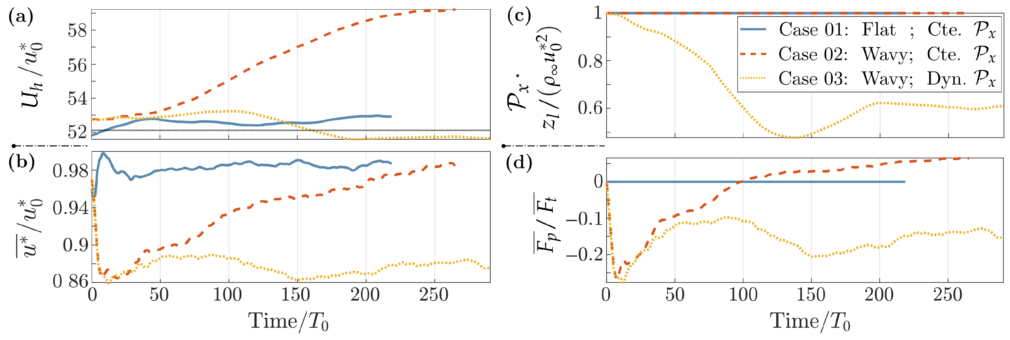
Three cases are presented, initializing with freestream velocity resolved as $u_{ref0}=52.11u_0^{*}$ (see initialization in Section 2.1.3). Case 01 is the reference, with flat-bottom BC and a constant ${\mathcal{P}}_x={\rho }_{\infty }{u}_0^{*2}/z_l$. Case 02 introduces the monochromatic wave (${\mathrm{WA}}_0=60$), still keeping a constant ${\mathcal{P}}_x$. Case 03 considers this same wave, but also the dynamic ${\mathcal{P}}_x$ modeler here proposed, with target velocity ($u_{ref}$) equal to the initial $u_{ref0}$.

• Results

Time histories are shown in Figure 3, by employing sliding-time statistics with long average periods $t_{avg}=75T_0$. The normalized mean wind velocity in the last cell layer ($U_h/u_0^{*}$, with $U_h=\overline{|\langle {\tilde{\mathit{u}}}_h\rangle |}$) is shown in Figure 3a. In the flat-bottom case (Case 01), the freestream velocity deviates $\sim 2$% from its initial value. The wave acts as an additional driving force dragging the wind above. Therefore, without a diminishing ${\mathcal{P}}_x$ balancing the additional momentum transferred to the wind, the freestream velocity is greatly augmented by the introduction of the wave in Case 02, reaching values ∼14% higher than $u_{ref}$. In Case 03, the dynamic ${\mathcal{P}}_x$ algorithm is activated, and the target velocity $u_{ref}$ is shown as the horizontal line in the figure. With this approach, the freestream velocity deviates only ∼1% from the target, when $t>200T_0$ in Case 03.

The resolved friction velocity ($\overline{u^{*}}$) is normalized by its nominal value in Figure 3b. Concerning Case 02, the wave first leads to a rapid drop in the friction velocity, which later returns towards $u_0^{*}$ over large periods. Employing the dynamic ${\mathcal{P}}_x$ in Case 03, the friction velocity does not recover the nominal value but is kept at ∼$0.88u_0^{*}$.

Both the freestream and friction velocities of Figure 3a,b reveal a persistent transient regime for Case 02, which in fact has not completely converged after the 2 million time steps, and during the period of $250T_0$ shown in the figures. The transient regime is significantly mitigated in Case 03 with the dynamic ${\mathcal{P}}_x$ method, which presents relatively slight velocity variations over the whole computation, reaching a statistically steady regime for $t>200T_0$.

The homogeneous pressure gradient is shown in Figure 3c: Constant and equal to $1/z_l$ for Cases 01 and 02; dynamic and slowly evolving in Case 03, which converges towards ${\mathcal{P}}_x\sim 0.6/z_l$ for $t>200T_0$. The transient ${\mathcal{P}}_x$ in Case 03 is responsible for keeping the quasi-steady wind and friction velocities.

Neglecting viscous effects, the WI stress integrates into the form drag in the lower surface, and is responsible for the vertical transfer of momentum between waves and wind [14,15]. If the waves travel sufficiently fast (large WA) with a significant wave slope, the upward transfer is such that the wave signature emerges as a low-level jet, characterized by a local maximum in the wind velocity profiles [16,17,18].

The momentum transfer between the wave and the wind is evaluated in the non-dimensional form drag (per surface unit) $\overline{F_p}/\overline{F_t}$, which also exhibits a transient behavior in Figure 3d. While Case 03 converges towards $\overline{F_p}/\overline{F_t}\sim -15$% for $t>200T_0$, Case 02 continues to increase after its sudden drop and minimum occurring at $t\sim 10T_0$. Moreover in Case 03, $\overline{F_p}<0$ and the momentum transfers exclusively upwards, but for Case 02, the form drag changes the sign, and upon becoming positive, it indicates a downward (wind-to-wave) momentum transfer for $t>100T_0$.

Interestingly for Case 02, the freestream velocity converges towards the wave phase velocity in the last instants of Figure 3a, when $U_h/c=99.5$%. This means that Miles’ critical height, where $U=c$ [3,74,75], is being brought inside the computational domain.

The mean wind and turbulence profiles in the last instants of the depicted evolution are presented in Figure 4. In the longitudinal velocities of Figure 4a, the speed-up of Case 02 occurs through the whole extension of the domain, while in Case 03 the speed-up is restricted to lower altitudes.

Inferred from the velocity time histories in Figure 3a,b, the different wave ages between Cases 02 and 03 qualitatively justify the differences in the turbulent profiles of Figure 4b,c, where they are normalized by the resolved friction velocity $\overline{u^{*}}$. In the turbulent profiles, the disturbances previously reported in [52], for the TKE and the total shear stresses, are again observed in Figure 4, and increased in Case 03, where the WA is higher. A systematic WA comparison is presented in Section 5.

4. Flat-Bottom Application

In this section, we show that the proposed methodology preserves the self-similarity of turbulent statistics for flat-bottom cases while employing the dynamic ${\mathcal{P}}_x$ modeler to build varying wind initial conditions prior to Section 5. These flat-bottom references provide guidance for the evaluation of WI disturbances later on.

• Test Cases

Five cases are presented, varying the freestream velocity from its initial value. The dynamic ${\mathcal{P}}_x$ method is thus employed with varying target velocities: Cases [01, 02, 03, 04, 05] with target $u_{ref}=[0.75,0.90,1.00,1.10,1.25]u_{ref0}$, respectively, and with $u_{ref0}=52.11u_0^{*}$. The nominal friction velocity characterizing each case is thus $u_{ref}^{*}=u_{ref}/52.11$, and the corresponding characteristic time-scale is $T_{ref}=\lambda /u_{ref}^{*}$.

4.1. Evolution and Turbulent Profiles

Time histories are shown in Figure 5, by employing sliding-time statistics with short average periods $t_{avg}=75\times {10}^{-3}{T}_0$, in order to assess the different turbulence levels and periods that characterize the evolution of different quantities. The mean wind velocity in the last cell layer ($U_h$) is shown in Figure 5a, showing that it tends to the specified values ($u_{ref}$) depicted by the horizontal lines in the figure. The low level of fluctuations revealed for $U_h$ is consistent with the low turbulence level imposed by the upper BC.

The dynamic ${\mathcal{P}}_x$ is shown in Figure 5b. As expected, ${\mathcal{P}}_x$ evolves in larger periods than $U_h$, with its natural period imposed as $T_{\mathcal{P}}=77T_0$. The friction velocity is normalized by $u_{ref}^{*}$ in Figure 5c. As the last cell velocity approaches the target, the non-dimensional solution converges between the cases attesting to their self-similarity.

The vertical wind and turbulent profiles are shown in Figure 6. They provide further evidence that self-similarity is preserved since the cases almost perfectly collapse in the non-dimensional, mean longitudinal velocity $\overline{\langle \tilde{u}\rangle }/\overline{u^{*}}$, turbulence intensity (TI) TI${}_{\varphi \varphi }=\sqrt{\overline{\langle {\varphi }^{\prime }{\varphi }^{\prime }\rangle }}/\overline{\langle \tilde{u}\rangle }$, and total shear stresses $\overline{\langle {\tau }_{13}\rangle }/\left({\rho }_{\infty }\overline{u^{*2}}\right)$, shown respectively in Figure 6a–c.

4.2. Wind Velocity Profiles and Fitting

We applied a logarithmic fitting to the wind profiles, by introducing the effective friction velocity (${\alpha }_u\overline{u^{*}}$) and roughness length (${\alpha }_z{z}_0$), in Equation (15):

$$\begin{array}{c}\hfill {\overline{u}}_{FIT}={\displaystyle \frac{{\alpha }_u\overline{u^{*}}}{\kappa }}ln\left({\displaystyle \frac{z}{{\alpha }_z{z}_0}}\right),\end{array}$$

(15)

thus recovering the log law of Equation (6) when $[{\alpha }_u=1,{\alpha }_z=1]$. With parameters $\left[{\alpha }_u,{\alpha }_z\right]$, the fitting minimizes the RMS difference $RM{S}_{diff}$, defined in Equation (16) in an arbitrary region $z_{min}<z<z_{max}$.

$$\begin{array}{c}\hfill RM{S}_{diff}=\sqrt{{\displaystyle \frac{1}{n}}\sum _n\left[{\displaystyle \frac{{({\overline{u}}_{FIT}-\overline{\langle u\rangle })}^2}{{\overline{\langle u\rangle }}^2}}\right]},\forall \{n\mid z_{min}\le z_n\le z_{max}\}.\end{array}$$

(16)

This fitting is embedded in an adaptive procedure determining the log law region at $z_{min}\le z\le z_{max}$. Given the threshold $RM{S}_c$, and starting at $z_{max}$, the lower limit ($z_{min}$) descends while $RM{S}_{diff}<RM{S}_c$. Thus, the log law region is defined as the most extensive portion of the ABL below $z_{max}$, in which the log fitting error is less than $RM{S}_c=5\times {10}^{-3}$. Here $z_{max}=0.8L_0$ is fixed, in order to later guide the evaluation of WI disturbances in the lower part of the logarithmic region.

The logarithmic fitting is depicted in Figure 7, revealing different regions inside the domain. In the numerical inner surface layer, the modeled SGS stresses are significant. In the outer surface region, highly anisotropic turbulence dominates the shear flow, the SGS stresses become negligible with respect to the LES-resolved turbulence, and the longitudinal velocity is given by a log law profile; this so-called logarithmic region is observed above a numerical buffer region and below the outer layer. In the outer layer, the flow adapts to the freestream condition, turbulence vanishes, and the velocity profiles exhibit an almost linear behavior [52].

Considering the uncertainty as ($\pm 0.5$) the maximum variation between the cases, the described fitting leads to ${\alpha }_u=0.93\pm 0.03$ and ${\alpha }_z=0.43\pm 0.16$, with $z_{min}/L_0=0.03$.

5. Wave Age Variation

The proposed methodology is employed here to perform a systematic WA variation study in old seas ($48\le {\mathrm{WA}}_{ref}\le 79$), by varying the wind speed in the range $\pm 25\%$.

• Test Cases

The wavy bottom surface replaces the flat-bottom cases previously discussed in Section 4. A single monochromatic wave is considered, with $ka=0.2$ and $\lambda =L_0$. The varying wind conditions lead to nominal ${\mathrm{WA}}_{ref}=c/u_{ref}^{*}=[79,66,60,54,48]$, for Cases [01, 02, 03, 04, 05], respectively.

5.1. Time Histories

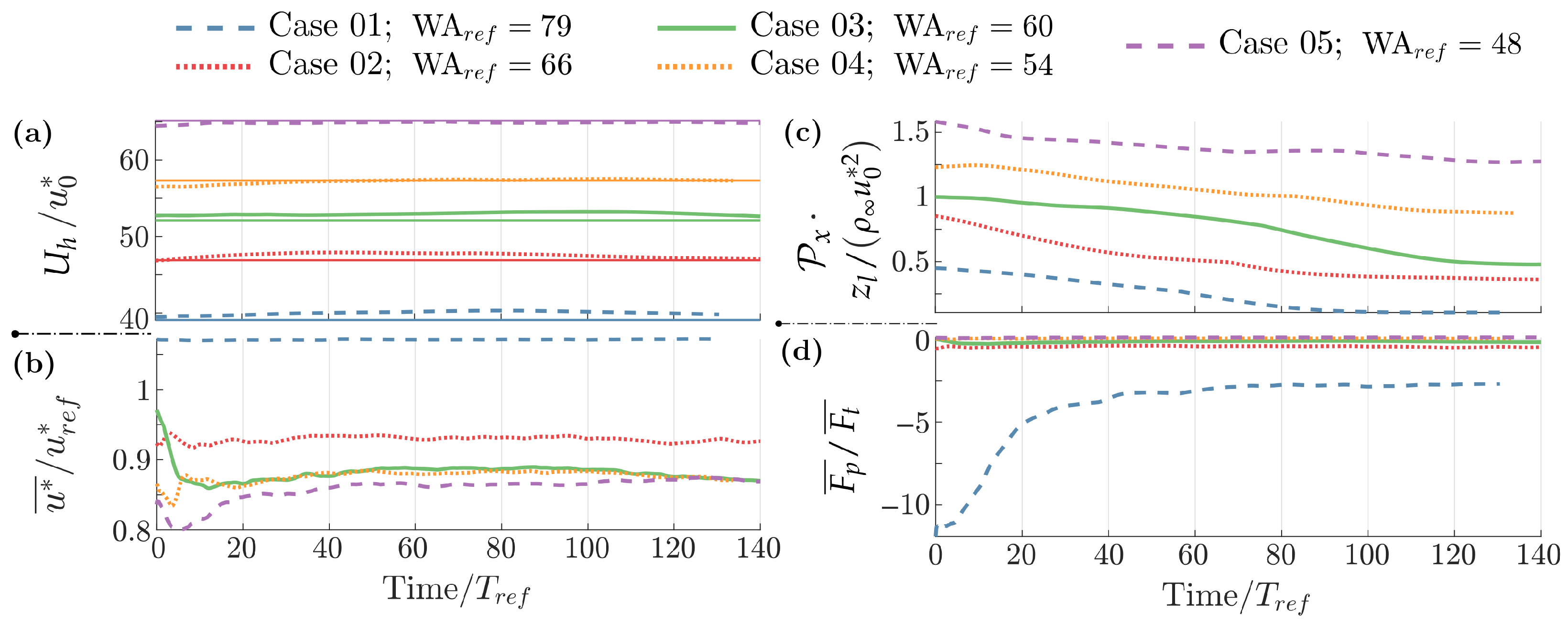
The normalized mean wind velocity in the upper cell layer ($U_h$) is shown in Figure 8a. The horizontal lines in the figure depict the target velocities ($u_{ref}$). The highest discrepancy observed between $U_h$ and $u_{ref}$ is 3.1% by the middle of the evolution depicted for Case 01 (highest WA). In the last steps of the evolution, the discrepancy in Case 01 is still the highest and drops to 1.9%.

Contrary to the flat-bottom cases of Section 4, here $\overline{u^{*}}/u_{ref}^{*}$ becomes a function of the WA as observed in Figure 8b. Except for Case 01, the friction velocities drop with respect to the reference values, and the discrepancy is larger with larger reference velocities, becoming the largest in Cases 03, 04, and 05, with 13% deviation in the last steps of Figure 8b. Cases 03, 04, and 05 converge to the same values of $\overline{u^{*}}/u_{ref}^{*}$, which suggests a saturation for this ratio at the lowest WA considered, but further investigations are needed with broader WA ranges to confirm this trend.

The dynamic pressure gradient decreases due to the introduction of the wave, evolving as reported in Figure 8c. The form drag evolution is depicted in Figure 8d, revealing an exponential trend between Cases 01 and 05 that is further evaluated in Section 5.3. The quantities presented in

Table 1. The parameters of Figure 8 probed in the final time-step, and the corresponding reference values.

Case ID	${\displaystyle \frac{{\mathit{u}}_{\mathit{ref}}}{{\mathit{u}}_{\mathit{ref}0}}}$	${\displaystyle \frac{{\mathit{U}}_{\mathit{h}}-{\mathit{u}}_{\mathit{ref}}}{{\mathit{u}}_{\mathit{ref}}}}$	${\displaystyle \frac{{\mathcal{P}}_{\mathit{x}}·{\mathit{z}}_{\mathit{l}}}{{\mathit{\rho }}_{\mathit{\infty }}{\mathit{u}}_0^{*2}}}$	${\displaystyle \frac{\overline{{\mathit{u}}^{*}}}{{\mathit{u}}_{\mathit{ref}}^{*}}}$	WA${}_{\mathit{ref}}$	WA
1	0.75	1.85%	0.107	1.073	79	74
2	0.90	0.18%	0.361	0.926	66	72
3	1.00	1.24%	0.479	0.871	60	68
4	1.10	−0.04%	0.876	0.870	54	62
5	1.25	−0.49%	1.270	0.869	48	55

were evaluated in the final time-step of the evolution depicted in Figure 8.

5.2. Wind Velocity Profiles

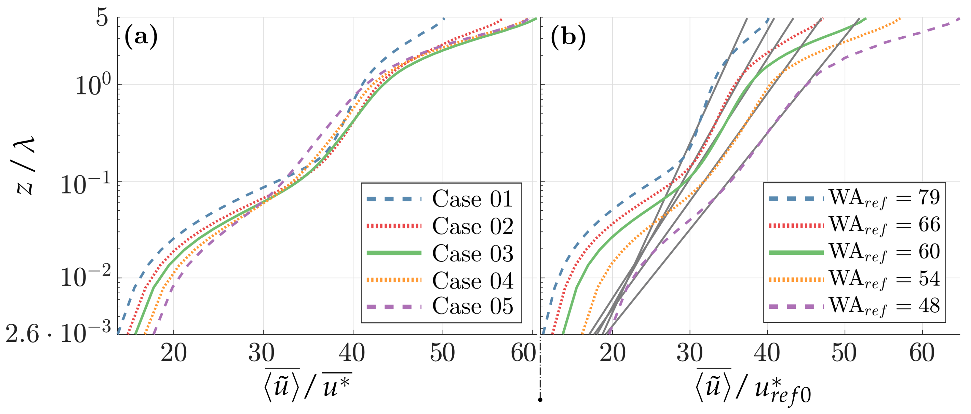
The normalized wind profiles vary substantially between the cases, as shown in Figure 9a. The log law functions were fitted to the outer surface layer, according to the procedure described in Section 4.2. The fitting is here depicted in Figure 9b, with the solution reported in

Table 2. Log law-fit of Equation (15) to the outer surface layer: Optimal $\left[{\alpha }_u,{\alpha }_z\right]$, for $RM{S}_{diff}<3\times {10}^{-3}$, in $\left[z_{min},z_{max}\right]$, with $z_{max}=0.8\lambda$. $\left[{\alpha }_u,{\alpha }_z\right]=\left[1,1\right]$ recovers the BC of Equation (6).

iCase	WA${}_{\mathit{ref}}$	${\mathit{\alpha }}_{\mathit{u}}$	${\mathit{\alpha }}_{\mathit{z}}$	${\mathit{z}}_{\mathit{min}}/\mathit{\lambda }$
1	79	0.94	0.03	0.18
2	66	1.40	4.16	0.14
3	60	1.48	9.41	0.11
4	54	1.57	20.09	0.08
5	48	1.58	29.01	0.06
Flat	–	0.93 ± 0.03	0.43 ± 0.16	0.03

. The flat cases presented in Section 4.2 appear in the tables with the case-averaged values, and the uncertainties are taken as ($\pm 0.5$) the maximum variation between the flat-bottom cases.

In Figure 9b, it can be seen that in the (numerical) inner surface layer, the effective roughness length increases with increasing WA, and the buffer region extends higher in the domain. As a consequence in Table 2, one observes a clear trend of increasing $z_{min}$ with increasing WA. The logarithmic layer is thus confined to higher altitudes, suggesting an increased WBL height scaling with the WA.

Contrary to the inner region, but as expected from the literature [34], in the outer surface layer the effective roughness length decreases with increasing WA, as seen in Table 2. Except for Case 01 (highest WA), there are strong friction velocity disturbances (${\alpha }_u$) due to the wave incidence; between Cases 2 and 5 these vary from 40% to 58%, compared to only −6% in Case 01 and the uncertainty of ±3%.

5.3. Form Drag Parametrization

In the literature [12,38,53,76], the form drag $F_p$ (evolution in Figure 8d), or the growth rate parameter $\beta =2F_p/\left[u^{*2}{\left(ka\right)}^2\right]$, are usually assumed as dependent on the WA. Nevertheless, different definitions are then employed to define such a WA parameter [76]. We discussed different definitions of friction velocity. So in order to evaluate these relations, Figure 10a presents $\overline{F_p}/\overline{F_t}$ as either dependent on the resolved WA $=c/u^{*}$ (in red circles), or the nominal WA${}_{ref}=c/u_{ref}^{*}$ (in blue dots). Defining the nominal WA${}_{ref}$, $u_{ref}^{*}$ scales linearly to the target velocity $u_{ref}$, and $u_{ref}$ approximates the resolved freestream velocity ($U_h$) with better than 3% accuracy.

Exponential functions are fitted to the data. The fitting of constants A and B from Equation (17) applies to the slopes of the LES results shown in Figure 10a, evaluated in the middle of the intervals by a first-order finite difference, as denoted by the dots and circles in Figure 10b. The constant part of the approximation function (C in Equation (17)) is set to match exactly the solution in Case 03.

The fitting is denoted by the curves, and the quality of the procedure is evaluated by the $R^2$ criterion in Figure 10a,b. It is thus seen that in the present formulation, the form drag scales better with the nominal WA${}_{ref}$ ($R^2=0.99$), which characterizes the non-disturbed flow, and thanks to the ${\mathcal{P}}_x$ modeler used here it scales with the freestream velocity. Therefore, the form drag dependency on the WA${}_{ref}$ is given here by the fitting denoted as blue full lines in Figure 10a, obtained with parameters $[A=1.07\times {10}^{-1},B=6.75\times {10}^{-6},C=2.04\times {10}^{-1}]$.

$$\begin{array}{c}\hfill \begin{array}{c}\hfill {\displaystyle \frac{F_p}{F_t}}=-{\displaystyle \frac{Bexp[A·\mathrm{WA}]}{A}}+C\end{array}\end{array}$$

(17)

5.4. Turbulent Profiles

• Turbulent Normal Stresses

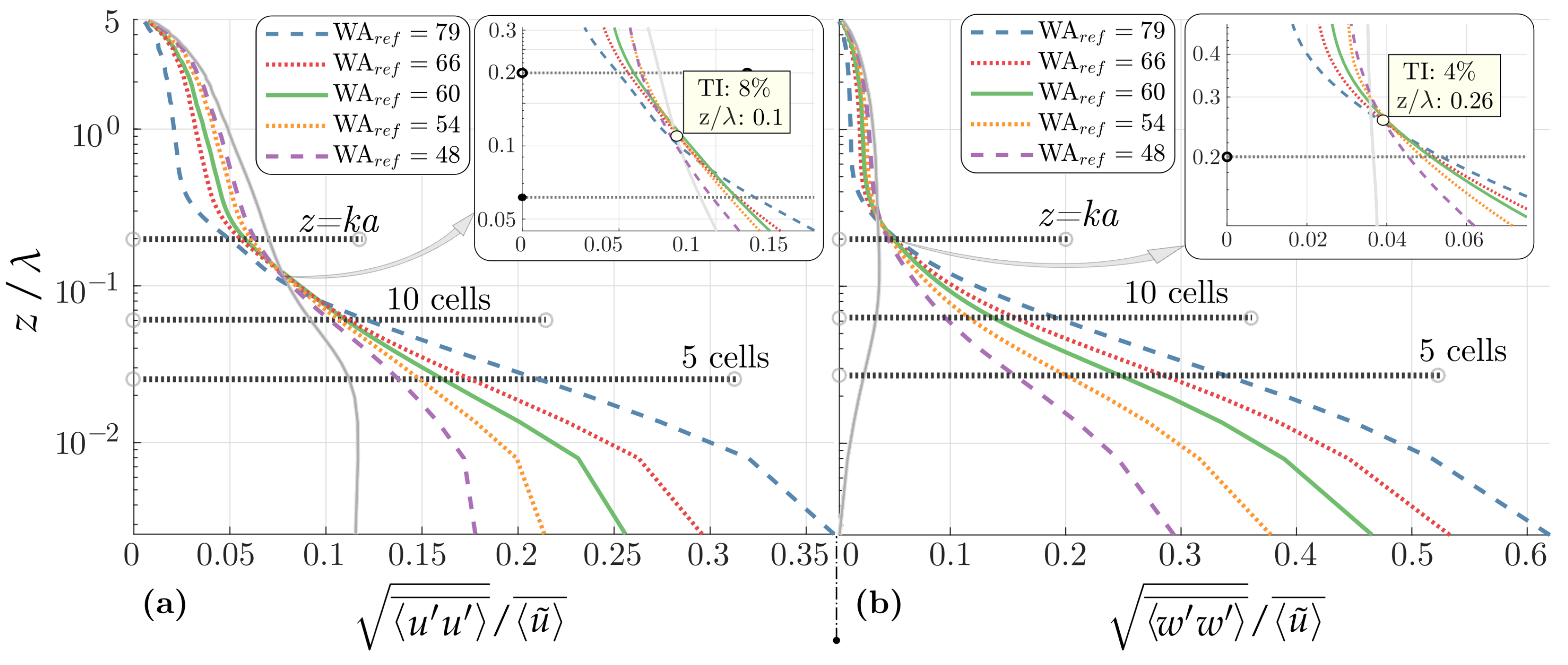
The TI for longitudinal and vertical velocities are shown, respectively, in Figure 11a,b. In these figures, the colored lines depict the wavy Cases 01 to 05 as described in the legend, and the light gray lines depict the reference, case averaged flat-bottom solution. As usual, the variances are strongly enhanced close to the surface due to the introduction of the wave. Farther away from the surface, on the contrary, TI diminishes. As the WA increases, the disturbances are amplified, the variances increase close to the surface, and diminish in the outer region.

A striking feature revealed in Figure 11 is that for each TI${}_{uu}$ and TI${}_{ww}$, the point where the cases intersect with each other and the flat case solution remains almost constant: $z/\lambda =0.1$ for TI${}_{uu}$ in Figure 11a, and $z/\lambda =0.26$ for TI${}_{ww}$ in Figure 11b. Clearly, the enhancement in TI close to the surface is due to the existence of WI motions, shown in Paskin et al. [52] to propagate higher in the WBL for the vertical velocities. TKE budget analyses reported in the literature (c.f. [19,77]) indicate that the decrease in TI on the outer region is due to an imbalance between the turbulent and pressure transport terms in the lower region, bringing turbulent motions from the outer layer into the WBL.

• Turbulent Shear stresses

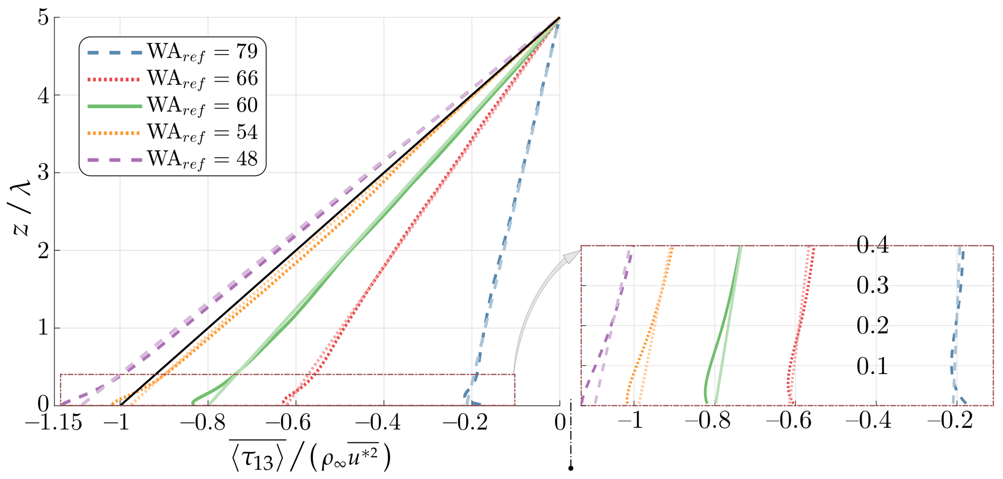
The total shear stresses ($\overline{\langle {\tau }_{13}\rangle }$) are shown in Figure 12, where they exhibit a mostly linear behavior with varying slopes between the cases. A linear fitting was applied to each profile and is shown with transparent lines in the figure. The theoretical flat-bottom solution is a straight line, denoted in black, varying from $\overline{\langle {\tau }_{13}\rangle }={\rho }_{\infty }\overline{u^{*2}}$ at the bottom ($S_{z-}$), to $\overline{\langle {\tau }_{13}\rangle }=0$ at the top ($S_{z+}$). Due to the waves, and a non-negligible WI form drag, the total shear stress profiles depart from other values rather than ${\rho }_{\infty }\overline{u^{*2}}$ in the bottom, and evolve until vanishing in the upper boundary. The fitted profiles evolve from the surface with the values given in

Table 3. Linear fitting for $\overline{\langle {\tau }_{13}\rangle }\left(z\right)$, from Figure 12. $\overline{\langle {\tau }_{13}\rangle }\left(z_l\right)=0$. The table gives the values of $\overline{\langle {\tau }_{13}\rangle }\left(0\right)$.

Case ID	WA${}_{\mathit{ref}}$	$\overline{\langle {\mathit{\tau }}_{13}\rangle }\left(0\right)/\overline{{\mathit{u}}^{*2}}$
1	79	−0.21
2	66	−0.62
3	60	−0.80
4	54	−0.98
5	48	−1.10

, and are null when $z=z_l$. The stresses deviate from the linear behavior in the (numerical) buffer region, zoomed in the lower right corner of Figure 12.

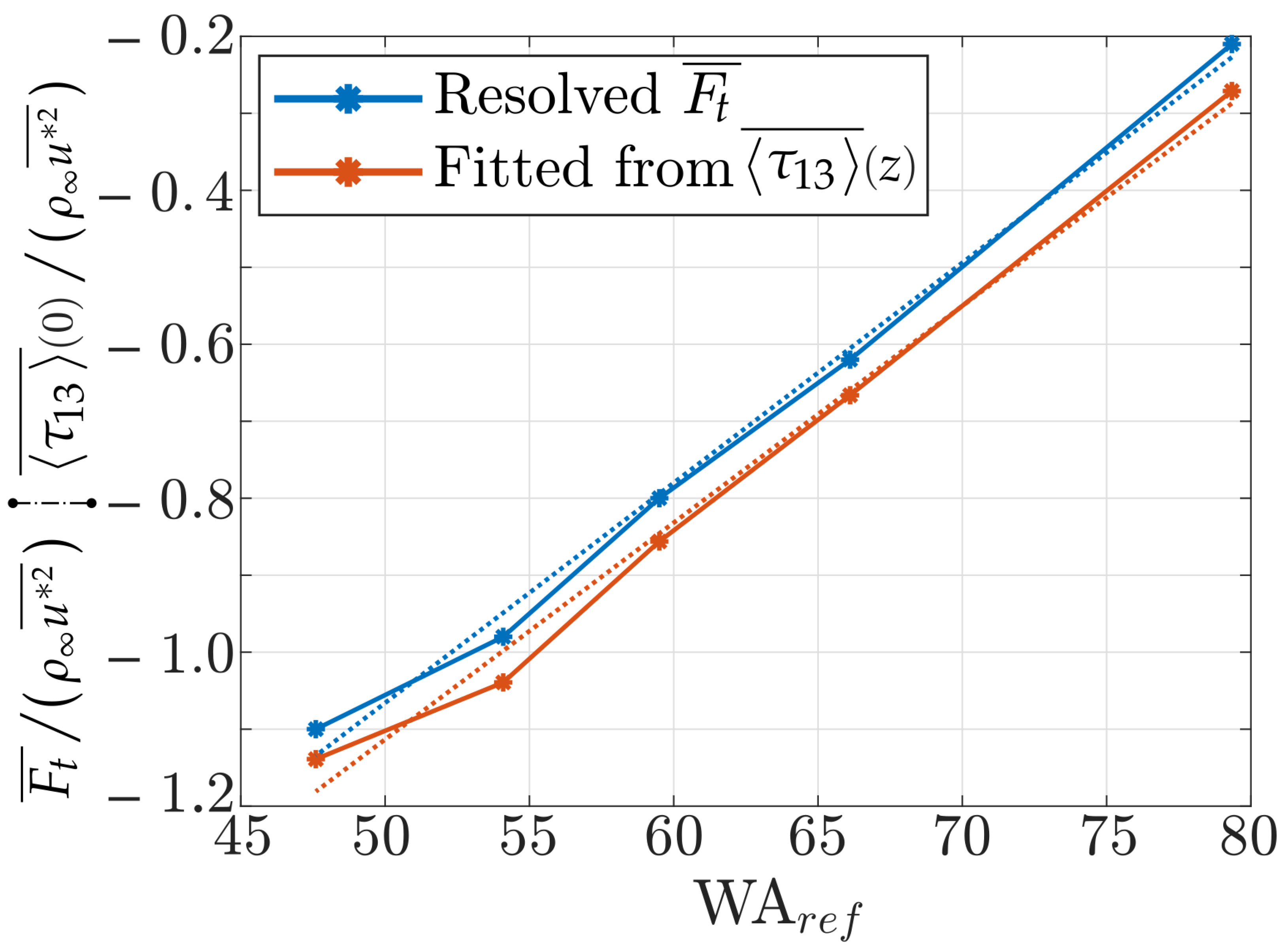
The form drag ($\overline{F_p}$) was previously discussed in Figure 8d. In Cases 01 and 02, the drag is negative, and the waves are expected to grow. However, in Case 02, the value is very close to zero, and not surprisingly the shear stresses closely approach the flat-bottom solution in Figure 12. The pressure drag is clearly the determining factor that imposes the slope of the profiles in Figure 12. To clarify this relationship, Figure 13 compares the dependence of $\overline{F_t}$ on the WA${}_{ref}$, as obtained from either: $\overline{F_t}=\overline{F_p}+\overline{F_f}$, with $\overline{F_f}={\rho }_{\infty }\overline{u^{*2}}$, resolved $\overline{u^{*}}$ reported in Table 1, and $\overline{F_p}/\overline{F_t}$ depicted in Figure 10a; or from the fitted value of $\overline{F_t}=\overline{\langle {\tau }_{13}\rangle }(z=0)$, reported in Table 3. There is a very good agreement between the predictions, for which linear fittings appear as dotted lines in the figures. Nevertheless, there is a small but persistent bias between these estimations, probably induced by the linear fitting employed for the $\overline{\langle {\tau }_{13}\rangle }$ profile (in Figure 12, leading to Table 3).

The fitting coefficients for $\overline{F_t}/\overline{u^{*2}}$ and $\overline{\langle {\tau }_{13}\rangle }\left(0\right)/\overline{u^{*2}}$ in Figure 13 are given in

Table 4. The total drag ($\overline{F_t}$) as a function of the WA${}_{ref}$ is approximated as $\overline{F_t}/\overline{u^{*2}}=A·$WA${}_{ref}+B$, with coefficients given below.

Case ID	A	B
Resolved $\overline{F_t}$	2.84 $\times {10}^{-2}$	−2.54
Fitted from $\overline{\langle {\tau }_{13}\rangle }\left(z\right)$	2.84 $\times {10}^{-2}$	−2.48

. The offset between the curves in Figure 13 is observed in the 2% discrepancy in coefficient B, which represents either: an offset of 3% (1.84 of 60) in the WA${}_{ref}$; or an offset of 5% (0.05 of 1) in $\overline{F_t}/\overline{u^{*2}}$.

6. Discussion

6.1. Reviewing the Mathematical Formulation of a Physical MABL in LES

We considered the mathematical formulation of a marine atmospheric boundary layer (MABL) in large eddy simulation(s) (LES), in a simplified framework summarized in Section 6.2. The MABL is bounded below by ocean waves traveling in the free surface, and above by the freestream. These physics translate in LES as a moving bottom with no-slip–no-penetration, and an upper surface with free-slip–no-penetration boundary conditions (BCs). Ocean waves carry momentum upwards or downwards in the MABL, but wave-induced (WI) disturbances are supposedly limited to the free surface vicinity [10,11,12,13]. Nevertheless, case-dependent WI stresses combined with a free-slip upper BC in LES allow a varying Wind Speed (WS) profile across the vertical extension of the domain. The WI disturbance of the freestream is unlikely to occur in the MABL but is intrinsic to the mathematical formulations previously employed in LES (c.f. [49,51,53,57]).

Atmospheric Reynolds averaged numerical simulations (RANS) employ a no-slip upper BC to drive the flow in the domain, which precisely imposes the mean freestream velocity in the upper boundary (c.f. [78]). Imposing no-slip upper BCs in DNS (c.f. [38,42]) or LES (c.f. [58]) formulations differ from an atmospheric setup, as a secondary boundary layer develops attached to the top boundary of the domain. Instead, in atmospheric LES the flow is driven by large-scale forces. These large-scale forces exist in the MABL coupling the meso- to the micro-scales, both as a large-scale pressure gradient and the Coriolis force (c.f. [66]). In the vast majority of previous LES studies of micro-scale wind–wave interactions the large-scale forces were considered as a constant [47,48,49,50,51,53,54,55,56,57,60]. However, there is no physical reason for this assumption (c.f. [59,62,65]), since the large-scale conditions could well vary in scales much larger than the computational domain.

6.2. A Simplified Framework

The simplified numerical framework exploited in this paper and detailed in Section 2.1 can be summarized as follows: Wind and waves propagate in the same direction, in a prismatic domain representing a wind tunnel; a single monochromatic wave is prescribed and not resolved, in order to prevent the free surface evolution under the wind forcing; old seas are considered, as the waves propagate rapidly compared to the wind; buoyancy forces are neglected, thus representing neutral stratification conditions; turbulence is fully developed in the air, so that the molecular viscosity can be neglected; Coriolis forces are neglected, as we focus on the airflow close to the sea surface; the test cases are exploited once the solution has converged to a statistically stationary regime.

6.3. Evaluating Standard LES Formulations of the MABL

Considering the simplified framework adopted, the results for a standard LES formulation are presented in Section 3 as Cases 01 (flat-bottom reference) and 02 (wavy bottom reference). Case 02 reveals a certain number of artificial features unlikely to occur in the physical MABL. Notably, the mean velocities increased to the upper boundary, and the freestream velocity is greatly augmented due to the incidence of the wave. The freestream velocity increases up to a moment where it drags back the propagating wave. The downward momentum transfer that occurs is characteristic of young seas, even though we attempted to reproduce old seas conditions in this simulation. The normalized total shear stress converges towards the flat-bottom case. These processes reveal a long transient regime, while the flow adapts all the way up to the top boundary. Most interestingly and hardly a coincidence, the freestream self-adapts towards a condition where its velocity matches the wave phase velocity ($U_h/c=99.5$%), thus bringing Miles’ critical height (c.f. [3,74,75]) inside the numerical domain.

Considering the dynamic pressure gradient proposed herein and employed in Case 03 of Section 3, these artificial features disappear. The friction velocity self-adapts to the appearance of the wave, but the freestream velocity is kept constant. A steady state regime is rapidly reached. The momentum flux occurs exclusively upwards. The WI disturbance in the wind velocity profile is kept confined to lower altitudes.

6.4. Large-Scale Dynamically Evolving Pressure Gradient Modeler

In the physical MABL and as long as the boundary layer height is sufficiently distant from the ocean (in neutral or unstable stratification conditions), it is more likely that the large-scale pressure gradient (traveling instantaneously in incompressible flows) will adapt to maintain a freestream velocity, rather than that, the freestream velocity will vary to maintain a constant large-scale pressure gradient condition.

In order to maintain an undisturbed freestream, while resolving arbitrary WI stresses, we developed a general method to control the wind speed at a certain height in the numerical domain (Section 2.2). To achieve this, an artificial evolution equation was built for the spatially-homogeneous large-scale pressure gradient: ${\mathcal{P}}_x=\partial \mathcal{P}/\partial x$. As an innovation in the wind–wave interaction studies, ${\mathcal{P}}_x$ is thus allowed to evolve in time, restricted to scales much larger than the resolved ones. Unlike other solutions developed for inland applications [61,62,64,66], this methodology does not require previous knowledge about the instantaneous characteristics of a wind speed and considers a continuous evolution of ${\mathcal{P}}_x$. This method was employed here to control the wind speed on the upper boundary but can be easily generalized to arbitrary heights in the domain.

The evolution equation built is a second-order PDE, also known as the rigid-body equation of motion, employed to dynamically filter the fluid momentum conservation equations. The mass-spring-damper system is critically damped ($\zeta =1$) to preserve stability. Large natural periods ($T_{\mathcal{P}}$) ensure that ${\mathcal{P}}_x$ responds to motions occurring at scales much larger than the numerical domain. In flat-bottom applications (Section 4), this guided the convergence of freestream velocities to a certain target $u_{ref}$, over periods comparable to $T_{\mathcal{P}}$. The convergence to a steady state regime was favored, and the normalized turbulence statistics were shown to be invariant to different values of $u_{ref}$ (setup ranging by $\pm 25$%).

6.5. WI Disturbances and WA Parametrization

In the wavy bottom applications exploited here in Section 5, the quasi-steady state was maintained in the freestream with better than 3% accuracy. This allowed a systematic WA variation study ($48\le {\mathrm{WA}}_{ref}\le 79$) by varying the wind speed, in old seas, and under the prescription of a single monochromatic wave with moderate to high steepness ($ka=0.2$). This canonical scenario was chosen for demonstration purposes, as it provides a critical evaluation of WI momentum stresses in the atmosphere.

The WI disturbances are usually assumed as a function of the WA parameter. However, many different definitions have been employed in the literature to define the WA, either in terms of the friction velocity or the wind speed measured at an arbitrary height [79]. We have shown that when ${\mathcal{P}}_x$ is kept constant, the friction velocity converges towards undisturbed values in LES. Employing the dynamic ${\mathcal{P}}_x$ modeler, on the contrary, the friction velocity exhibits a strong dependency on the WA. Therefore if the WA is defined as a function of the resolved friction velocity, one establishes a circular dependency between these parameters. This problem is likely to occur in the physical MABL, as there is no reason to assume that the friction velocity remains constant with a changing sea-state condition.

A definite parametrization of WI disturbances remains beyond the scope of the present study, but we performed these studies to attest to the self-consistency of the methodology presented. To evaluate the behavior of different WA definitions, we fitted the form drag as either a function of the reference or the resolved WA. The WA${}_{ref}$ characterizing the non-disturbed or freestream flow was found to be more accurate to describe the observations. When evaluating the turbulent profiles, this parametrization also provided a reasonable linear approximation of the height-dependent shear stresses.

Other observations are in accordance with the literature and attest to the robustness of the methodology proposed. The region of validity of the logarithmic wind profiles displaces upwards with increasing WA [19,80]. In the outer surface layer the effective roughness length decreases with increasing WA [34,37]. Turbulence intensities (TI) are increased in the WBL due to the WI fluctuations and diminish above the WBL due to the downward transport of turbulent fluctuations [19,77].

7. Conclusions

We employed LES to study micro-scale wind–wave interactions, proposing a new method to control the wind speed above arbitrary stresses in the bottom. When the sea-state condition is modified in LES, the wind speed at the top of the domain ($U_h$) self-adapts to the changes in wave-induced (WI) stresses that carry momentum downwards (wind-to-wave) or upwards (wave-to-wind) through the domain. However, a constant $U_h$ is desired to correctly compare different test cases submitted to an undisturbed freestream condition.

In order to maintain an undisturbed freestream while resolving arbitrary WI stresses, we developed a general method to control the wind speed at a certain height in the numerical domain. To achieve this, an evolution equation was built for the spatially-homogeneous large-scale pressure gradient: ${\mathcal{P}}_x$. In flat-bottom applications, this guided the convergence of freestream velocities to a certain target $u_{ref}$. The convergence to a steady state regime was favored, and the normalized turbulence statistics were shown to be invariant to different values of $u_{ref}$ (setup ranging by $\pm 25$%). In wavy bottom applications, the quasi-steady state was maintained in the freestream with better than 3% accuracy. This allowed a systematic WA variation study ($48\le {\mathrm{WA}}_{ref}\le 79$) by varying the wind speed, in old seas, and under the prescription of a single monochromatic wave. This canonical scenario provides a critical evaluation of WI momentum stresses in the atmosphere. This methodology provides self-consistent WA parametrizations from LES and enables valuable analyses of wind–wave interactions.

The proposed parametrizations present a qualitative description of physical processes and trends. They are not intended to be taken in a quantitative manner due to the limited resources in terms of grid resolution. Future work will address more realistic conditions and finer grid resolutions, in order to present more quantitative descriptions of WI disturbances from LES. Moreover, in future work, the dynamic large-scale forcing modeler will be employed to enhance the comparison of physical and numerical experiments, by employing the wind speed control at the measurement height, rather than at the upper boundary.

References

1. Thomson, W. Hydrokinetic Solutions and Observations. Philos. Mag. 1871, 42, 326–378. [Google Scholar] [CrossRef]
2. Jeffreys, H. On the formation of water waves by wind. Proc. R. Soc. Lond. 1925, 107, 189–206. [Google Scholar]
3. Miles, J.W. On The Generation Of Surface Waves By Shear Flows, PartI. J. Fluid Mech. 1957, 3, 185–204. [Google Scholar] [CrossRef]
4. Phillips, O.M. On The Generation Of Waves By Turbulent Wind. J. Fluid Mech. 1957, 2, 417–445. [Google Scholar] [CrossRef]
5. Belcher, S.E.; Hunt, J.C.R. Turbulent Shear Flow Over Slowly Moving Waves. J. Fluid Mech. 1993, 251, 109–148. [Google Scholar] [CrossRef]
6. Edson, J.B.; Zappa, C.J.; Ware, J.A.; McGillis, W.R.; Hare, J.E. Scalar flux profile relationships over the open ocean. J. Geophys. Res. Ocean. 2004, 109, C8. [Google Scholar] [CrossRef] [Green Version]
7. Grare, L.; Lenain, L.; Melville, W.K. Wave-Coherent Airflow and Critical Layers over Ocean Waves. J. Phys. Oceanogr. 2013, 43, 2156–2172. [Google Scholar] [CrossRef]
8. Bourras, D.; Branger, H.; Reverdin, G.; Marié, L.; Cambra, R.; Baggio, L.; Caudoux, C.; Caudal, G.; Morisset, S.; Geyskens, N.; et al. A New Platform for the Determination of Air–Sea Fluxes (OCARINA): Overview and First Results. J. Atmos. Ocean. Technol. 2014, 31, 1043–1062. [Google Scholar] [CrossRef] [Green Version]
9. Tamura, H.; Drennan, W.M.; Collins, C.O.; Graber, H.C. Turbulent Airflow and Wave-Induced Stress Over the Ocean. Bound.-Layer Meteorol. 2018, 169, 47–66. [Google Scholar] [CrossRef]
10. Paskin, L.; Conan, B.; Perignon, Y.; Aubrun, S. Evidence of Ocean Waves Signature in the Space–Time Turbulent Spectra of the Lower Marine Atmosphere Measured by a Scanning LiDAR. Remote Sens. 2022, 14, 3007. [Google Scholar] [CrossRef]
11. Hristov, T. Mechanistic, empirical and numerical perspectives on wind-waves interaction. Procedia IUTAM 2018, 26, 102–111. [Google Scholar] [CrossRef]
12. Harris, J.A.; Belcher, S.E.; Street, R.L. Linear dynamics of wind waves in coupled turbulent air–water flow. Part 2. Numerical model. J. Fluid Mech. 1996, 308, 219–254. [Google Scholar] [CrossRef]
13. Ayet, A.; Chapron, B. The Dynamical Coupling of Wind-Waves and Atmospheric Turbulence: A Review of Theoretical and Phenomenological Models. Bound.-Layer Meteorol. 2022, 183, 1–33. [Google Scholar] [CrossRef]
14. Yousefi, K.; Veron, F. Boundary layer formulations in orthogonal curvilinear coordinates for flow over wind-generated surface waves. J. Fluid Mech. 2020, 888, A11. [Google Scholar] [CrossRef]
15. Ayet, A. Air-Sea Momentum Fluxes in the Vicinity of the Sea Surface: A Theoretical Study of the Coupling between Turbulence and Wind-Waves. Ph.D. Thesis, Université de Bretagne Occidentale, Brest, France, 2020. [Google Scholar]
16. Smedman, A.; Högström, U.; Bergström, H.; Rutgersson, A.; Kahma, K.K.; Pettersson, H. A case study of air-sea interaction during swell conditions. J. Geophys. Res. Ocean. 1999, 104, 25833–25851. [Google Scholar] [CrossRef]
17. Harris, D.L. The Wave-Driven Wind. J. Atmos. Sci. 1966, 23, 688–693. [Google Scholar] [CrossRef]
18. Hanley, K.E.; Belcher, S.E. Wave-Driven Wind Jets in the Marine Atmospheric Boundary Layer. J. Atmos. Sci. 2008, 65, 2646–2660. [Google Scholar] [CrossRef] [Green Version]
19. Sjöblom, A.; Smedman, A.S. The turbulent kinetic energy budget in the marine atmospheric surface layer. J. Geophys. Res. Ocean. 2002, 107, 6–18. [Google Scholar] [CrossRef]
20. Cifuentes-Lorenzen, A.; Edson, J.B.; Zappa, C.J. Air–Sea Interaction in the Southern Ocean: Exploring the Height of the Wave Boundary Layer at the Air–Sea Interface. Bound.-Layer Meteorol. 2018, 169, 461–482. [Google Scholar] [CrossRef]
21. Chalikov, D.; Babanin, A.V. Parameterization of Wave Boundary Layer. Atmosphere 2019, 10, 686. [Google Scholar] [CrossRef] [Green Version]
22. Semedo, A.; Saetra, Ø.; Rutgersson, A.; Kahma, K.K.; Pettersson, H. Wave-Induced Wind in the Marine Boundary Layer. J. Atmos. Sci. 2009, 66, 2256–2271. [Google Scholar] [CrossRef]
23. Liu, C.; Li, X.; Song, J.; Zou, Z.; Huang, J.; Zhang, J.A.; Jie, G.; Wang, J. Characteristics of the Marine Atmospheric Boundary Layer under the Influence of Ocean Surface Waves. J. Phys. Oceanogr. 2022, 52, 1261–1276. [Google Scholar] [CrossRef]
24. Janssen, P.A.E.M.; Breivik, Ø.; Mogensen, K.; Vitart, F.; Alonso-Balmaseda, M.; Bidlot, J.R.; Keeley, S.; Leutbecher, M.; Magnusson, L.; Molteni, F. Air-sea interaction and surface waves. ECMWF Tech. Memo. 2013, 712, 1–34. [Google Scholar]
25. Li, H.; Claremar, B.; Wu, L.; Hallgren, C.; Körnich, H.; Ivanell, S.; Sahlée, E. A sensitivity study of the WRF model in offshore wind modeling over the Baltic Sea. Geosci. Front. 2021, 12, 101229. [Google Scholar] [CrossRef]
26. Rezaeiha, A.; Pereira, R.; Kotsonis, M. Fluctuations of angle of attack and lift coefficient and the resultant fatigue loads for a large Horizontal Axis Wind turbine. Renew. Energy 2017, 114, 904–916. [Google Scholar] [CrossRef]
27. Leroy, V.; Gilloteaux, J.C.; Lynch, M.; Babarit, A.; Ferrant, P. Impact of aerodynamic modeling on seakeeping performance of a floating horizontal axis wind turbine. Wind Energy 2019, 22, 1019–1033. [Google Scholar] [CrossRef]
28. Kalvig, S.; Gudmestad, O.T.; Winther, N. Exploring the gap between ‘best knowledge’ and ‘best practice’ in boundary layer meteorology for offshore wind energy. Wind Energy 2014, 17, 161–171. [Google Scholar] [CrossRef]
29. Obukhov, A.M. Turbulence in an Atmosphere with a Non-Uniform Temperature. Bound.-Layer Meteorol. 1946, 2, 7–29. [Google Scholar] [CrossRef]
30. Monin, A.S.; Obukhov, A.M. Basic Laws of Turbulent Mixing in the Surface Layer of the Atmosphere. Contrib. Geophys. Inst. Acad. Sci. USSR 1954, 24, 163–187. [Google Scholar]
31. Edson, J.B.; Fairall, C.W. Similarity Relationships in the Marine Atmospheric Surface Layer for Terms in the TKE and Scalar Variance Budgets. J. Atmos. Sci. 1998, 55, 2311–2328. [Google Scholar] [CrossRef]
32. Hristov, T.; Ruiz-Plancarte, J. Dynamic Balances in a Wavy Boundary Layer. J. Phys. Oceanogr. 2014, 44, 3185–3194. [Google Scholar] [CrossRef]
33. Charnock, H. Wind stress on a water surface. Q. J. R. Meteorol. Soc. 1955, 81, 639–640. [Google Scholar] [CrossRef]
34. Donelan, M.A.; Dobson, F.W.; Smith, S.D.; Anderson, R.J. On the Dependence of Sea Surface Roughness on Wave Development. J. Phys. Oceanogr. 1993, 23, 2143–2149. [Google Scholar] [CrossRef]
35. Edson, J.B.; Jampana, V.; Weller, R.A.; Bigorre, S.P.; Plueddemann, A.J.; Fairall, C.W.; Miller, S.D.; Mahrt, L.; Vickers, D.; Hersbach, H. On the Exchange of Momentum over the Open Ocean. J. Phys. Oceanogr. 2013, 43, 1589–1610. [Google Scholar] [CrossRef] [Green Version]
36. Patton, E.G.; Sullivan, P.P.; Kosović, B.; Dudhia, J.; Mahrt, L.; Žagar, M.; Marić, T. On the Influence of Swell Propagation Angle on Surface Drag. J. Appl. Meteorol. Climatol. 2019, 58, 1039–1059. [Google Scholar] [CrossRef] [Green Version]
37. Porchetta, S.; Temel, O.; Muñoz Esparza, D.; Reuder, J.; Monbaliu, J.; van Beeck, J.; van Lipzig, N. A new roughness length parameterization accounting for wind–wave (mis)alignment. Atmos. Chem. Phys. 2019, 19, 6681–6700. [Google Scholar] [CrossRef] [Green Version]
38. Sullivan, P.P.; McWilliams, J.C.; Moeng, C.H. Simulation of turbulent flow over idealized water waves. J. Fluid Mech. 2000, 404, 47–85. [Google Scholar] [CrossRef] [Green Version]
39. Yang, D.; Shen, L. Characteristics of coherent vortical structures in turbulent flows over progressive surface waves. Phys. Fluids 2009, 21, 125106. [Google Scholar] [CrossRef]
40. Yang, D.; Shen, L. Direct-simulation-based study of turbulent flow over various waving boundaries. J. Fluid Mech. 2010, 650, 131–180. [Google Scholar] [CrossRef] [Green Version]
41. Yang, D.; Shen, L. Simulation of viscous flows with undulatory boundaries. Part I: Basic solver. J. Comput. Phys. 2011, 230, 5488–5509. [Google Scholar] [CrossRef]
42. Druzhinin, O.A.; Troitskaya, Y.I.; Zilitinkevich, S.S. Direct numerical simulation of a turbulent wind over a wavy water surface. J. Geophys. Res. Ocean. 2012, 117, C11. [Google Scholar] [CrossRef]
43. Yang, Z.; Deng, B.Q.; Shen, L. Direct numerical simulation of wind turbulence over breaking waves. J. Fluid Mech. 2018, 850, 120–155. [Google Scholar] [CrossRef]
44. Deskos, G.; Ananthan, S.; Sprague, M.A. Direct numerical simulations of turbulent flow over misaligned traveling waves. Int. J. Heat Fluid Flow 2022, 97, 109029. [Google Scholar] [CrossRef]
45. Stoll, R.; Gibbs, J.A.; Salesky, S.T.; Anderson, W.; Calaf, M. Large-Eddy Simulation of the Atmospheric Boundary Layer. Bound.-Layer Meteorol. 2020, 177, 541–581. [Google Scholar]
46. Chanprasert, W.; Sharma, R.; Cater, J.; Norris, S. Large Eddy Simulation of wind turbine fatigue loading and yaw dynamics induced by wake turbulence. Renew. Energy 2022, 190, 208–222. [Google Scholar] [CrossRef]
47. Henn, D.S.; Sykes, R.I. Large-eddy simulation of flow over wavy surfaces. J. Fluid Mech. 1999, 383, 75–112. [Google Scholar] [CrossRef]
48. Sullivan, P.P.; Edson, J.B.; Hristov, T.; McWilliams, J.C. Large-Eddy Simulations and Observations of Atmospheric Marine Boundary Layers above Nonequilibrium Surface Waves. J. Atmos. Sci. 2008, 65, 1225–1245. [Google Scholar] [CrossRef] [Green Version]
49. Sullivan, P.P.; McWilliams, J.C.; Patton, E.G. Large-Eddy Simulation of Marine Atmospheric Boundary Layers above a Spectrum of Moving Waves. J. Atmos. Sci. 2014, 71, 4001–4027. [Google Scholar] [CrossRef] [Green Version]
50. Hara, T.; Sullivan, P.P. Wave Boundary Layer Turbulence over Surface Waves in a Strongly Forced Condition. J. Phys. Oceanogr. 2015, 45, 868–883. [Google Scholar] [CrossRef] [Green Version]
51. Cathelain, M. Development of a Deterministic Numerical Model for the Study of the Coupling between an Atmospheric Flow and a Sea State. Ph.D. Thesis, Ecole Centrale de Nantes (ECN), Nantes, France, 2017. [Google Scholar]
52. Paskin, L.; Perignon, Y.; Conan, B.; Aubrun, S. Numerical study on the Wave Boundary Layer, its interaction with turbulence and consequences on the wind energy resource in the offshore environment. J. Phys. Conf. Ser. 2020, 1618, 062046. [Google Scholar] [CrossRef]
53. Yang, D.; Meneveau, C.; Shen, L. Dynamic modelling of sea-surface roughness for large-eddy simulation of wind over ocean wavefield. J. Fluid Mech. 2013, 726, 62–99. [Google Scholar] [CrossRef]
54. Yang, D.; Meneveau, C.; Shen, L. Effect of downwind swells on offshore wind energy harvesting—A large-eddy simulation study. Renew. Energy 2014, 70, 11–23. [Google Scholar] [CrossRef]
55. Yang, D.; Meneveau, C.; Shen, L. Large-eddy simulation of offshore wind farm. Phys. Fluids 2014, 26, 025101. [Google Scholar] [CrossRef]
56. Hao, X.; Shen, L. Wind–wave coupling study using LES of wind and phase-resolved simulation of nonlinear waves. J. Fluid Mech. 2019, 874, 391–425. [Google Scholar] [CrossRef]
57. Hao, X.; Cao, T.; Shen, L. Mechanistic study of shoaling effect on momentum transfer between turbulent flow and traveling wave using large-eddy simulation. Phys. Rev. Fluids 2021, 6, 054608. [Google Scholar] [CrossRef]
58. Cao, T.; Shen, L. A numerical and theoretical study of wind over fast-propagating water waves. J. Fluid Mech. 2021, 919, A38. [Google Scholar] [CrossRef]
59. Hao, X.; Shen, L. Large-eddy simulation of gusty wind turbulence over a travelling wave. J. Fluid Mech. 2022, 946, A8. [Google Scholar] [CrossRef]
60. Deskos, G.; Lee, J.C.Y.; Draxl, C.; Sprague, M.A. Review of Wind–Wave Coupling Models for Large-Eddy Simulation of the Marine Atmospheric Boundary Layer. J. Atmos. Sci. 2021, 78, 3025–3045. [Google Scholar] [CrossRef]
61. Pedersen, J.G.; Kelly, M.; Gryning, S.E.; Brümmer, B. The effect of unsteady and baroclinic forcing on predicted wind profiles in Large Eddy Simulations: Two case studies of the daytime atmospheric boundary layer. Meteorologische Zeitschrift 2013, 22, 661–674. [Google Scholar] [CrossRef] [Green Version]
62. Basu, S.; Vinuesa, J.; Swift, A. Dynamic LES Modeling of a Diurnal Cycle. J. Appl. Meteorol. Climatol. 2008, 47, 1156–1174. [Google Scholar] [CrossRef] [Green Version]
63. Nielson, J.; Bhaganagar, K. Capturing Day-to-day Diurnal Variations in Stability in the Convective Atmospheric Boundary Layer Using Large Eddy Simulation. Open Atmos. Sci. J. 2018, 12, 107–131. [Google Scholar] [CrossRef]
64. Allaerts, D.; Quon, E.; Draxl, C.; Churchfield, M. Development of a Time–Height Profile Assimilation Technique for Large-Eddy Simulation. Bound.-Layer Meteorol. 2020, 176, 329–348. [Google Scholar] [CrossRef]
65. Draxl, C.; Allaerts, D.; Quon, E.; Churchfield, M. Coupling Mesoscale Budget Components to Large-Eddy Simulations for Wind-Energy Applications. Bound.-Layer Meteorol. 2021, 179, 73–98. [Google Scholar] [CrossRef]
66. Pimont, F.; Dupuy, J.L.; Linn, R.R.; Sauer, J.A.; Muñoz-Esparza, D. Pressure-Gradient Forcing Methods for Large-Eddy Simulations of Flows in the Lower Atmospheric Boundary Layer. Atmosphere 2020, 11, 1343. [Google Scholar] [CrossRef]
67. Stieren, A.; Gadde, S.N.; Stevens, R.J. Modeling dynamic wind direction changes in large eddy simulations of wind farms. Renew. Energy 2021, 170, 1342–1352. [Google Scholar] [CrossRef]
68. Fenton, J.D. A fifth-order Stokes theory for steady waves. J. Waterw. Port Coastal Ocean. Eng. 1985, 111, 216–234. [Google Scholar] [CrossRef] [Green Version]
69. Spiegel, E.A.; Veronis, G. On The Boussinesq Approximation For A Compressible Fluid. Astrophys. J. 1960, 131, 442. [Google Scholar] [CrossRef]
70. Moeng, C.H. A Large-Eddy-Simulation Model for the Study of Planetary Boundary-Layer Turbulence. J. Atmos. Sci. 1984, 41, 2052–2062. [Google Scholar] [CrossRef]
71. Thomas, P.D.; Lombard, C.K. Geometric Conservation Law and Its Application to Flow Computations on Moving Grids. AIAA J. 1979, 17, 1030–1037. [Google Scholar] [CrossRef]
72. Kleppner, D.; Kolenkow, R. An Introduction to Mechanics, 1st ed.; Cambridge University Press: Cambridge, UK, 2010; pp. 410–440. [Google Scholar]
73. Georgi, H. The Physics of Waves, 1st ed.; Prentice Hall: Englewood Cliffs, NJ, USA, 1993; pp. 1–52. [Google Scholar]
74. Lighthill, M.J. Physical interpretation of the mathematical theory of wave generation by wind. J. Fluid Mech. 1962, 14, 385–398. [Google Scholar] [CrossRef]
75. Hristov, T.S.; Miller, S.D.; Friehe, C.A. Dynamical coupling of wind and ocean waves through wave-induced air flow. Nature 2003, 422, 55–58. [Google Scholar] [CrossRef] [PubMed]
76. Donelan, M.; Babanin, A.; Young, I.; Banner, M. Wave-Follower Field Measurements of the Wind-Input Spectral Function. Part II: Parameterization of the Wind Input. J. Phys. Oceanogr. 2006, 36, 1672–1689. [Google Scholar] [CrossRef]
77. Högström, U.; Smedman, A.; Sahleé, E.; Drennan, W.M.; Kahma, K.K.; Pettersson, H.; Zhang, F. The Atmospheric Boundary Layer during Swell: A Field Study and Interpretation of the Turbulent Kinetic Energy Budget for High Wave Ages. J. Atmos. Sci. 2009, 66, 2764–2779. [Google Scholar] [CrossRef] [Green Version]
78. O’Sullivan, J.; Archer, R.; Flay, R. Consistent boundary conditions for flows within the atmospheric boundary layer. J. Wind. Eng. Ind. Aerodyn. 2011, 99, 65–77. [Google Scholar] [CrossRef]
79. Donelan, M.A.; Drennan, W.M.; Magnusson, A.K. Nonstationary Analysis of the Directional Properties of Propagating Waves. J. Phys. Oceanogr. 1996, 26, 1901–1914. [Google Scholar] [CrossRef]
80. Mastenbroek, C. Wind–Wave Interaction. Ph.D. Thesis, TU Delft, Delft, The Netherlands, 1996. [Google Scholar]
Figure 1. The wind tunnel-like simulation in Cartesian coordinates. Wind and waves are aligned to the x axis. The domain is bounded below by an arbitrary single-valued wave, and above by the freestream. The flow is driven by the large-scale pressure gradient P / x .
Atmosphere 13 02012 g001
Figure 2. The Mass-Spring-Damper system ruling the evolution of the longitudinal pressure gradient P x = P / x , according to Equation (12).
Atmosphere 13 02012 g002
Figure 3. Time histories of non-dimensional: (a) wind speed at S z + ; (b) friction velocity; (c) large-scale pressure gradient; and (d) form drag. Averaged with t a v g = 75 T 0 . Case 01: Flat bottom with constant P x , as the reference. Case 02: Wavy bottom with constant P x . Case 03: Wavy bottom with the dynamic P x modeler.
Atmosphere 13 02012 g003
Figure 4. Height-dependent wind and turbulence profiles averaged with t a v g = 75 T 0 . Pilot application. (a) longitudinal velocity; (b) total shear stress; (c) total turbulent kinetic energy (TKE).
Atmosphere 13 02012 g004
Figure 5. Time histories of non-dimensional: (a) wind speed at S z + , with target values denoted in the horizontal lines; (b) large-scale pressure gradient; (c) friction velocity. Averaged with t a v g = 75 × 10 3 T 0 . Flat-bottom application.
Atmosphere 13 02012 g005
Figure 6. Height-dependent wind and turbulence profiles averaged with t a v g = 75 T 0 . Flat-bottom application. (a) longitudinal velocity; (b) turbulence intensity (TI); (c) total shear stress. The normalizing friction velocity is resolved, as obtained from Equation (8).
Atmosphere 13 02012 g006
Figure 7. Wind longitudinal velocity profiles, with different colors for Cases 01 to 05 of the flat-bottom application. The log law fitting to the outer surface layer (by Equation (15)) is shown with transparent lines.
Atmosphere 13 02012 g007
Figure 8. Time histories of non-dimensional: (a) wind speed at S z + , with target values denoted in the horizontal lines; (b) friction velocity; (c) large-scale pressure gradient; and (d) form drag. Averaged with t a v g = 75 T 0 . Wavy bottom application.
Atmosphere 13 02012 g008
Figure 9. Longitudinal velocity profiles averaged with t a v g = 75 T 0 . (a) Normalized by the resolved friction velocity. (b) Normalized by the reference friction velocity; with logarithmic profiles fitted to the outer region, depicted in black transparent lines.
Atmosphere 13 02012 g009
Figure 10. Wave age dependency (Resolved WA, or Nominal WA r e f ) and fitting of the normalized form drag. The LES results are shown in dots and circles, and the fittings are given by full and dot-dashed lines. (a) Form drag and the exponential fitting in linear scale. (b) The negative signs of the slopes in the log scale are evaluated between the intervals of (a). A linear fit applies to the log of the slopes in (b), and integrates into the exponential in (a). The fitting quality was evaluated by the R 2 criterion.
Atmosphere 13 02012 g010
Figure 11. Turbulence intensity (TI) profiles averaged with t a v g = 75 T 0 . TI for longitudinal and vertical velocity fluctuations, in (a) and (b), respectively. The light gray lines represent the case averaged flat-bottom solution. The zoomed regions depict the intersections between the curves.
Atmosphere 13 02012 g011
Figure 12. Total shear stress, averaged with t a v g = 75 T 0 . Linear fittings are shown as transparent lines, parameterized according to Table 3. The black line represents the theoretical flat-bottom solution. The fitting is less accurate in the near-wall region, zoomed in the lower right corner.
Atmosphere 13 02012 g012
Figure 13. Normalized total drag as a function of the reference WA r e f . Comparison between the resolved value, and the one extrapolated from the linear fitting depicted in Figure 12. Here, a linear fitting applies to F t ¯ ( WA r e f ) , and is shown with dotted lines in the figure. The fitting coefficients are given in Table 4.
Atmosphere 13 02012 g013