Abstract
At the surface of the earth, the available radiative energy Rn is distributed between the ground heat flux and the sensible and latent heat fluxes according to the surface energy balance (SEB) equation. In the past decades, most attempts to measure the individual terms of this equation have revealed a non-closure problem, regardless of the site of observation or period of the year. Today, no definitive answer has been provided to this question. In general, it is suspected that the sensible and latent heat fluxes (H and LvE, respectively) that are calculated with the eddy-covariance technique are underestimated. This paper suggests two additional terms that should be considered in the SEB equation, which are based on thermodynamic considerations. They are directly related to H and LvE and appear to be interesting candidates for explaining (at least in part) the non-closure of the SEB. The distribution of the correction between H and LvE varies as a function of the Bowen ratio B. The correction relative to H is dominant for values of B that are greater than 0.2 and represents more than 80% of the total correction for values greater than unity. The impact of these corrections on the SEB closure was tested on a large set of observations from 24 FLUXNET sites around the world with different vegetation types. The closure defect, which is about 17% in the original dataset, is reduced to about 3% with the proposed corrections.
1. Introduction
The radiative energy available at the continental surface is distributed among different terms according to the surface energy balance (SEB) equation. In its simplest form, this equation reads as follows (e.g., Cuxart et al., 2015 [1]):
Each of the four terms in Equation (1) can be independently measured so that its closure can be evaluated. In general, a so-called “imbalance term” (Imb) must be added to the equation, because equilibrium between the left and right terms is not achieved. The Imb term contains both the contribution of omitted terms in the simplified equation and the uncertainties related to the observations and data processing. Omitted terms include heat storage in the canopy and energy consumed by the photosynthetic activity of vegetation, additional terms related to secondary circulations that are not captured by fixed-point observations, and horizontal fluxes divergence as well as vertical/horizontal advection when processes in the layer between the surface and the observation height cannot be neglected. Other uncertainties are based on instrumental errors and flaws in the data processing used to convert the raw observations into energy fluxes. In some complex situations, the 1D simple approach presented above is not sufficient and the budget of a volume must be undertaken, including part of the soil and the whole canopy layer. All this is detailed, for example, in the review paper of Mauder et al. [2].
There is an extensive amount of literature on energy balance closure. Most of these papers conclude that the left-hand side of Equation (1) is larger than the right-hand side, even when the components of the Imb, which can be estimated, are taken into account. This is especially observed during the daytime period when energy fluxes are the highest. Therefore, the most commonly reason invoked for this lack of closure is an underestimation of the sensible and/or latent heat flux.
The issue of imbalance was raised several decades ago. In the 1980s, Leuning et al. [3] reported that, over an arid area, H + LvE only accounted for 81% of Rn − G. The authors attributed the difference (in part) to loss due to the limited frequency range used to calculate heat fluxes by eddy correlation (EC) and to misalignment of sensors in the mean flow. Based on the observed Rn − G values, Desjardins [4] proposed correcting the EC-calculated H and LvE by ~15% to compensate for the covariance lost in the time series filtering. The author postulated that EC fluxes of other parameters (especially CO2 fluxes) should be corrected by the same amount as the loss is not flux-dependent but is due to the methodology used to compute the covariance. During the FIFE campaigns (1987 and 1989), several sites were equipped for the observation of the surface energy balance (Kanemasu et al., 1997 [5]), but the achievement of its closure was controversial. However, Panin et al. [6] revealed a considerable imbalance for these campaigns that they attributed to spatial heterogeneity. Barr et al. [7] reported an 11% underestimation of (H + LvE) EC values observed in 1988 on a North American forest. From these pioneering studies, papers reporting a closure of the SEB with EC heat fluxes are rare. We can mention Jacobs et al. [8] who achieved 96% closure on a grassland site in the Netherlands, or Leuning et al. [9] for whom energy balance closure is possible with careful attention to measurements and data processing. However, in general, the remaining imbalance was more in the range of 10–20%, as reported in review papers by Foken [10], Foken et al. [11] or Mauder et al. [2].
After the pioneering studies, the question of imbalance was explored in two ways. The first initiative was to construct an experiment dedicated to this question. Oncley et al. [12] described the EBEX-2000 campaign conducted on a uniform flood-irrigated cotton field with state-of-the-art instrumentation (including calibration and intercomparisons) and data processing. The imbalance was on the order of 10%, which the authors believed to be beyond the uncertainty resulting from possible sources of error. The second route taken to estimate the reality and magnitude of the SEB imbalance was to bring together observations from a large number of sites in a single data set, in contrast to previous studies (including EBEX) conducted for a dedicated area. Such a strategy was facilitated by the set-up of many FLUXNET sites around the world, motivated by carbon balance estimates in the context of climatic change, and which offered the observations required to estimate each term of the SEB equation. All these studies, gathering a number of sites ranging from 22 to 173, concluded that the H + LvE term was severely underestimated (Wilson et al. (2002) [13]; Hendricks-Franssen et al. (2010) [14]; Stoy et al. (2013) [15]).
Since these studies, we must now consider that the SEB imbalance is no longer an uncertainty but a systematic error. However, there is no consensus today on how the error is distributed between sensible and latent heat flux, nor on the main cause of this error, which explains why papers are still regularly published on this issue. Some of the most recent studies include Gao et al. (2020) [16], Li and Wang (2020) [17], Liu et al. (2021) [18] and Sun et al. (2021) [19].
In this paper, we suggest that two additional terms should be considered in the SEB equation. These terms are directly related to the sensible and latent heat fluxes and appear to be interesting candidates to explain (at least in part) the non-closure of the SEB. This study is presented in a 1D framework, i.e., with the assumption that the significant energy transfers occur only along the vertical direction. Furthermore, we will focus on the daytime period (H and LvE > 0, unstable conditions), as the energy involved is much higher than during the nighttime (stable) period. The paper is organized as follows. After a summary of the definition of sensible and latent heat fluxes and assessment of their EC formulation, we present the development of additional terms related to these fluxes. We then discuss the consequences on the SEB, according to the partition between the two fluxes. The impact of the corrections is tested on multi-year flux data collected on 24 sites of the FLUXNET network. The last part is the conclusion of the study and the consequences on other scalar fluxes.
2. Material and Methods
EC Fluxes
For any parameter χ, we adopt here the classical Reynolds decomposition of the instantaneous value between its average and fluctuation:
The kinematic turbulent flux of χ in the vertical direction is thus , where w is the vertical velocity of the air (positive upward), and the total vertical flux of χ is defined as:
The mass flux of water vapor just above the surface is thus defined as:
where qa is the water vapor concentration (in kg m−3). We know from the work of Webb et al. [20] that the first term of the right-hand side cannot be neglected as there is a non-zero mean vertical velocity resulting from the assumption that the total vertical mass flux of dry air is zero (, where ρd is the dry air density). The exact mathematical formulation of is quite complex (see Fuehrer and Friehe (2002) [21]), but because it is a correction term, we can adopt the following approximation:
where T is the absolute temperature. This amounts to making the approximation that ρ’/ρ ≈ −T’/T, where ρ is the air density. If we neglect the second (and higher) order terms in the corrections, E can be expressed with a very good approximation as follows [20]:
where rv is the water vapor mixing ratio.
Expressing the latent heat flux as LvE in the SEB equation is equivalent to assuming that all the water that is mechanically transferred upward and measured through the EC flux has been evaporated into the superficial soil layer; in other words, there is neither a lateral transfer of water vapor nor a significant accumulation/depletion between the surface and the measurement height.
For the sensible heat flux H, Fuehrer and Friehe [21] provided its full formulation, which is somewhat complex and requires the definition of reference temperatures. We start here from a simpler form based on the average heat transported along the vertical by up- and downdrafts:
where is the heat capacity of air at constant pressure (in J kg−1 K−1), the variations of which on the sample over which the flux is calculated can be neglected. After Reynolds decomposition and with the aforementioned assumptions regarding the mean vertical velocity and the similarity between density and temperature fluctuations, and assuming that , Equation (7) reads as follows:
This expression shows that the kinematic heat flux cannot be mathematically reduced to the single term of the covariance between the fluctuations of vertical wind and temperature. Given the temperature variance values observed in the atmospheric surface layer (ASL), the last term in Equation (8) is several orders of magnitude smaller than the first and can be neglected. The covariance was computed by Wyngaard and Coté [22]. The order of magnitude (see their Figure 11) was , where u* is the friction velocity. For a very wide range of heat flux and friction velocity values observed in the ASL, the second term in Equation (8) is at least two orders of magnitude smaller than the first. This leads to the commonly adopted form of the sensible heat flux:
3. Results
3.1. Additional Terms in the SEB Equation
In this section, we introduce two additional terms related to the sensible and latent heat fluxes. These terms, which must be considered in the SEB equation, have not yet been mentioned in the literature (to the best of our knowledge). They represent a certain amount of energy that cannot be drawn from anywhere else than the available reservoir constituted by the term Rn − G. We recall here that we only consider energy transfers in the vertical direction.
3.1.1. Additional Term Related to the Latent Heat Flux
Evaporation/transpiration results in the injection of a certain mass of water vapor into the atmosphere. These water molecules will occupy a volume that can be calculated according to perfect gas law. In the 1D framework that we consider in this paper, it is as if injected molecules would have to “nudge” the overlying air column. The energy WE (in Joules) consumed in this operation during a time interval δt can be expressed by the product of the air column weight F and the vertical dimension of the injected volume δh:
where S is the horizontal surface of the volume and P the surface atmospheric pressure. Because the SEB equation is established for a horizontal surface of 1 m2, we will adopt this value in the following. δh is related to evaporation through:
where ρv is the density an air parcel would have if it was only composed of water vapor molecules (without considering condensation). So, the perfect gas law leads to:
where R is the universal constant of perfect gas (R = 8.3 J K−1 mol−1) and mv is the water vapor molar mass (mv = 0.018 kg/mol). Combining Equation (10)–(12) leads to the following expression of the term related to the latent heat flux to be added to the SEB equation:
expressed in W m−2.
To provide an order of magnitude for standard meteorological conditions (T = 293 K and Lv = 2.501 106 − 2380(T − 273.15) J/kg), this term represents 5.5% of the latent heat flux.
It may seem strange at first sight that the pressure P does not explicitly appear in the expression of this additional term, as it represents the energy consumed to work against the atmospheric pressure. In fact, according to the perfect gas law, the volume occupied by the injected water molecules is inversely proportional to the atmospheric pressure, and the energy consumed, which is the product of the height of this volume and the weight of the air column, is the same regardless of the value of the pressure.
3.1.2. Additional Term Related to the Sensible Heat Flux
The sensible heat flux causes a heating of the atmospheric lower layer. According to the perfect gas law, this heating (δT) during a time interval δt results in an expansion of the corresponding volume of air V containing n moles, which can be expressed as:
with S = 1 m2 for the conditions of the SEB equation and δh expressing the dilatation along the vertical direction. We assume here that pressure variations can be neglected with respect to the other terms, which is justified as in the 1D approach adopted here, the pressure is numerically equal to the weight of the air column above a 1 m2 horizontal surface, and the sensible heat flux does not introduce additional molecules in the atmosphere.
Considering that the heating occurs in a layer of thickness h, we have:
where mair is the molecular weight of the air (mair ≈ 0.029 kg/mol, slightly varying with the air composition, in a particular water concentration). The variation of thickness can thus be expressed as:
If the heating is uniformly distributed in the layer of thickness h (typically, the atmospheric boundary layer, ABL), we have:
Note that the entrainment that occurs at the top of the ABL and contributes to its diurnal heating is not considered here, as it consists of a mechanical incorporation of existing warm air parcels into the ABL without any additional heat source, and the resulting overall expansion of the air mass is therefore zero. The expansion resulting from the surface sensible heat flux is therefore:
and the energy consumed to “raise” the air column is:
The term to be added to the SEB equation is therefore:
Knowing that ≈ 1004 J kg−1 K−1, we arrive at Δ(H) = 0.286 H, which is as high a value as the imbalance levels commonly published in the literature.
3.2. The Modified SEB Equation
Based on the above developments, the SEB equation originally presented is modified as follows:
The introduced “imbalance” terms (Imb = Δ(H) + Δ(LvE)) can thus be expressed as a fraction of the available energy (Rn − G) as:
Defining the Bowen ratio B as B = H/(LvE), we obtain:
where
Figure 1 shows the evolution of Fractional_Imb as a function of the Bowen ratio, for two temperatures (0 and 40 °C). The influence of temperature is marginal, except for low Bowen ratios (high evaporation and low sensible heat flux). The fractional imbalance varies from about 5% at low values of B to more than 20% for arid conditions (the maximum is 0.286 for conditions without evaporation/transpiration). For “standard” mid-latitude conditions with Bowen ratios in the range [0.2–0.6], the correction is of the order of 10%, which corresponds to the amount of non-closure observed, for example, during the EBEX experiment [12].
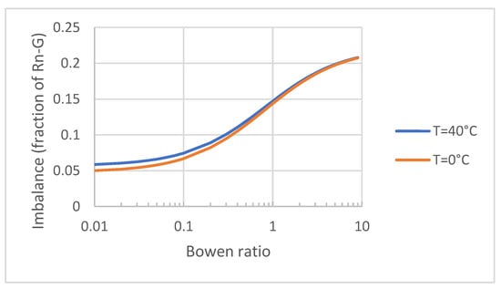
Figure 1.
Amount of additional terms in the SEB equation expressed as a fraction of the available energy, as a function of the Bowen ratio.
Figure 2 shows the proportion of the imbalance related to the sensible heat flux as a function of the Bowen ratio. The result does not significantly vary with temperature. The contribution of the sensible heat flux becomes dominant from values of the Bowen ratio that are higher than 0.21. This result is therefore in disagreement with several papers which proposed to compensate for the imbalance by distributing the correction between sensible and latent heat fluxes while maintaining the Bowen ratio. In contrast, Charuchittipan et al. [23] proposed a correction in which the respective contribution of sensible and latent heat flux to the buoyancy flux is maintained. The corresponding mathematical formulation is only slightly different from ours, and the values presented in their Figure 8 resemble those in Figure 2 here (with the difference that these authors use a logarithmic scale on their plot). However, the reasons they gave for this imbalance were completely different from those presented here as they focused on the extension of the frequency range used to calculate covariances to better capture secondary circulations.
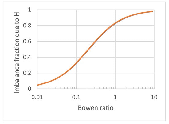
Figure 2.
Fraction of the total correction of the imbalance attributed to the sensible heat flux as a function of the Bowen ratio.
In the various studies reporting observations of SEB imbalance, there was no consensus on the allocation of the energy deficit between the sensible and latent heat flux. As mentioned by Twine et al. [24], keeping the same Bowen ratio for measured and corrected fluxes appears “reasonable”, but these authors recognized this was not proven. Imbalance has sometimes been observed to increase with instability (i.e., for small negative values of the Obukhov length Lo, see, e.g., Gao et al. [16]), but because instability relies on both H and the friction velocity u*, the impact on the heat flux is not straightforward to deduce, as pointed out by Hendricks-Franssen et al. [14]. On the other hand, Barr et al. [7] suggested that EC LvE was more underestimated than EC H. When secondary circulations (i.e., low-frequency transfers) are invoked to explain the SEB imbalance, it is argued that there is no similarity between heat and scalar transfers at low frequencies, such that the Bowen ratio is not kept at these frequencies. Furthermore, the imbalance does not automatically have the same proportion of sensible and latent heat flux (Foken, 2008 [10]; Foken et al., 2011 [11]). Similarly, Eder et al. [25] reported that the conserved Bowen ratio correction only works for Bowen ratios of the order of unity. As a consequence, and unlike that conducted in the paper by Desjardins [4], the estimate of the global imbalance cannot simply be passed on to other scalar fluxes (such as CO2). In their recent review paper, Mauder et al. [2] questioned the Bowen ratio conservation for corrected fluxes and suggested that H should be corrected by a larger percentage than LvE, providing support from large eddy simulation results that confirm the non-similarity of low frequency heat and scalar transfers.
3.3. Application to Observation Datasets
The corrections developed here have been applied to datasets collected at different observational sites and gathered in the FLUXNET network (https://fluxnet.org/data/, accessed on 17 October 2022). At FLUXNET sites, the eddy covariance technique is used to measure the cycling of carbon, water, and energy between the biosphere and atmosphere. The data used here come from the FLUXNET2015 Dataset. We selected 24 sites in different climates and with different vegetation types; we excluded sites with tall forests as the difference in the measurement height of the various terms of the energy budget equation may induce a source of imbalance, mainly related to the heat storage in the vegetation layer. We also chose datasets with a span time of more than 6 years. Because the corrections proposed in the paper are valid for the unstable period of the diurnal cycle, we restricted the data to those that satisfied the following conditions: H > 0, LvE > 0 and Rn − G > 0. The different sites and corresponding datasets are presented in Table 1, which shows their location, vegetation type, time period covered by the data, number of 30-min flux data used in the present study, and the references for a more complete description of the site and the data.

Table 1.
Characteristics of the FLUXNET sites and datasets used for the analysis: Site identifier on the FLUXNET portal (Site ID), country, coordinates, vegetation type, total period covered by the data, number of individual 30-min samples used is this study, and references for the site description and datasets.
For each site, we computed the imbalance by comparing the terms Rn − G and H + LvE, first with the values as stored in the FLUXNET dataset and then with the addition of the correction developed in the present study (Equation (13) and (20)). The results are summarized in Table 2. The imbalance of the uncorrected data was first estimated with the slope a of the linear regression Rn − G = a(H + LvE) + b. The value of a, averaged over the different sites is 0.743 (last row of Table 2). On average, the corresponding determination coefficient (R2) is 0.81. When we apply the corrections on the sensible and latent heat fluxes, the slope ac increases to 0.871 on average, which represents a significant improvement toward balance closure.
Table 2.
Characteristics of the linear regression between the available energy (Rn − G) and the sum of the sensible and latent heat fluxes for each of the 24 sites. The first column is the site identifier, and the last row contains the average values over the 24 sites. R2 is the determination coefficient, “BC” means before corrections, and “AC” refers to after the corrections presented in the text. The second and third columns contain the slopes of the linear regressions when Rn − G is computed as a function of the sum of the heat fluxes, while the last two columns present the geometric mean of the slopes.
However, as the determination coefficient is significantly less than unity, the result of the linear regression would depend on how it is computed. Considering the two variables X and Y and the two linear regressions Y = axX + bx and X = ayY + by, we know that ax # ay−1, as ax ay = R2. When considering the closure imbalance, there is no reason to favor one way of computing the regression over the other. In such a case, considering the geometric mean of the slopes of the two regressions (i.e., Y = axy X, with ) would be more appropriate. With such a definition, the corresponding slopes before and after correction are, on average, 0.825 and 0.967, respectively. The corrections allow us to achieve the balance of the energy budget to be within 3%.
4. Discussion and Conclusions
In this paper, we have proposed a development to take into account two additional terms in the SEB equation. These terms represent the energy consumed to work against the atmospheric pressure, to introduce into the lower layers the water vapor molecules resulting from evaporation for one part, and to allow the expansion resulting from the heating of the air for the other part. These two terms are expressed as a fraction of the sensible heat flux H and latent heat flux LvE. The first term is dominant for Bowen ratios greater than 0.2 and represents more than 80% of the correction for Bowen ratios greater than unity. When expressed as a fraction of the available energy Rn − G, the overall correction increases with the Bowen ratio and amounts to about 10% and 15% for Bowen ratios of about 0.3 and 1, respectively. These orders of magnitude are comparable to the imbalances reported in the literature.
We tested the impact of these corrections on a sampling of flux values collected at 24 FLUXNET sites, with different climate conditions and vegetation types. Even restricted to unstable periods, the selected dataset amounts to 1.286 106 30-min samples, which ensures the robustness of our results. Considering the geometric mean of the slopes computed in two ways (Rn − G vs. H + LvE and vice-versa), introducing the corrections on the sensible and latent heat fluxes presented here allows us to obtain a closure of the energy balance to be within 3%.
The present paper could therefore provide important elements to improve our understanding and knowledge of the imbalance issue that was highlighted several decades ago but is still not fully resolved. It is important to recall the simple framework in which we performed this study. We considered the simplest configuration, with a bare or short vegetated surface, in the 1D context (i.e., horizontal advection effects are neglected). All fluxes are considered at the interface between the surface and the atmosphere, i.e., the transfers occurring between this interface and the “real” level of observation (whether height in the air or depth in the soil) are neglected. Similarly, we have not considered the contribution of large-scale motions (i.e., at scales beyond the random turbulence), which is often invoked as a possible source of the observed imbalance. What we have shown in this paper does not mean that such contributions do not exist, but would certainly reduce their amount, and may call them into question as principal contributors to explain the imbalance, as it is frequently invoked in the literature (see, e.g., the recent paper of Liu et al. [18] and the related references they cite).
We have also placed ourselves in the context of the unstable/convective part of the diurnal cycle. This period of the day has larger values of the surface energy budget components than the stable/nocturnal period. Furthermore, there is no consensus on the existence of an imbalance for the stable period, nor on its magnitude. Regarding the correction we have calculated in relation to the sensible heat flux, we can expect a similar and opposite effect for the stable periods. Regarding the latent heat flux, it is not so straightforward, as a dew deposition would act as a restitution of energy; meanwhile, if evaporation is continuing (during windy nights for example), the effect would be identical to that of the daytime period.
With the magnitude of the additional terms presented in this paper, the closure of the energy balance certainly appears to be much more attainable. This would be a step toward reconciling the calculated EC fluxes with the available energy. A major consequence is the strengthening of our confidence in the EC scalar fluxes, especially CO2 fluxes, which are measured at a large number of sites around the world.
Funding
P. Durand is employed by the CNRS and resides at Université Paul Sabatier.
Informed Consent Statement
Not applicable.
Data Availability Statement
Not applicable. The data used in support of this study were downloaded from the FLUXNET site https://fluxnet.org/data/ (accessed on 9 October 2022).
Acknowledgments
We would like to thank all the people who have patiently and determinedly contributed to the huge and formidable FLUXNET data set over many years.
Conflicts of Interest
The authors declare no conflict of interest.
References
- Cuxart, J.; Conangla, L.; Jiménez, M.A. Evaluation of the surface energy budget equation with experimental data and the ECMWF model in the Ebro Valley. J. Geophys. Res. Atmos. 2015, 120, 1008–1022. [Google Scholar] [CrossRef]
- Mauder, M.; Foken, T.; Cuxart, J. Surface-energy-balance closure over land: A review. Bound.-Layer Meteorol. 2020, 177, 395–426. [Google Scholar] [CrossRef]
- Leuning, R.; Denmead, O.T.; Lang, A.R.G.; Ohtaki, E. Effects of heat and water vapor transport on eddy covariance measurement of CO2 fluxes. Bound.-Layer Meteorol 1982, 23, 209–222. [Google Scholar] [CrossRef]
- Desjardins, R.L. Carbon dioxide budget of maize. Agric. For. Meteorol. 1985, 36, 29–41. [Google Scholar] [CrossRef]
- Kanemasu, E.T.; Verma, S.B.; Smith, E.A.; Fritschen, L.J.; Wesely, M.; Field, R.T.; Kustas, W.P.; Weaver, H.; Stewart, J.B.; Gurney, R.; et al. Surface flux measurements in FIFE: An overview. J. Geophys. Res. 1992, 97, 18547–18555. [Google Scholar] [CrossRef]
- Panin, G.N.; Raabe, A.; Tetzlaff, G. Inhomogeneity of the land surface and problems in parametrization of surface fluxes in natural conditions. Theor. Appl. Climatol. 1998, 60, 163–178. [Google Scholar] [CrossRef]
- Barr, A.; King, K.M.; Gillespie, T.J.; Hartog, G.D.; Neumann, H.H. A comparison of Bowen ratio and eddy correlation sensible and latent heat flux measurements above deciduous forest. Bound.-Layer Meteorol. 1994, 71, 21–41. [Google Scholar] [CrossRef]
- Jacobs, A.F.G.; Heusinkveld, B.G.; Holtslag, A.A.M. Towards closing the surface energy budget of a mid-latitude grassland. Bound.-Layer Meteorol. 2008, 126, 125–136. [Google Scholar] [CrossRef]
- Leuning, R.; van Gorsel, E.; Massman, W.J.; Isaac, P.R. Reflections on the surface energy imbalance problem. Agric. For. Meteorol. 2012, 156, 65–74. [Google Scholar] [CrossRef]
- Foken, T. The energy balance closure problem: An overview. Ecol. Appl. 2008, 18, 1351–1367. [Google Scholar] [CrossRef]
- Foken, T.; Aubinet, M.; Finnigan, J.J.; Leclerc, M.Y.; Mauder, M.; Paw, U.K. Results of a panel discussion about the energy balance closure correction for trace gases. Bull. Am. Meteorol. Soc. 2011, 92, ES13–ES18. [Google Scholar] [CrossRef]
- Oncley, S.P.; Foken, T.; Vogt, R.; Kohsiek, W.; DeBruin, H.A.; Bernhofer, C.; Christen, A.; Gorsel, E.V.; Grantz, D.; Feigenwinter, C.; et al. The energy balance experiment EBEX-2000. Part I: Overview and energy balance. Bound.-Layer Meteorol. 2007, 123, 1–28. [Google Scholar] [CrossRef]
- Wilson, K.; Goldstein, A.; Falge, E.; Aubinet, M.; Baldocchi, D.; Berbigier, P.; Bernhofer, C.; Ceulemans, R.; Dolman, H.; Field, C.; et al. Energy balance closure at FLUXNET sites. Agric. For. Meteorol. 2002, 113, 223–243. [Google Scholar] [CrossRef]
- Franssen, H.H.; Stöckli, R.; Lehner, I.; Rotenberg, E.; Seneviratne, S.I. Energy balance closure of eddy-covariance data: A multisite analysis for European FLUXNET stations. Agric. For. Meteorol. 2010, 150, 1553–1567. [Google Scholar] [CrossRef]
- Stoy, P.C.; Mauder, M.; Foken, T.; Marcolla, B.; Boegh, E.; Ibrom, A.; Arain, M.A.; Arneth, A.; Aurela, M.; Bernhofer, C.; et al. A data-driven analysis of energy balance closure across FLUXNET research sites: The role of landscape-scale heterogeneity. Agric. For. Meteorol. 2013, 171–172, 137–152. [Google Scholar] [CrossRef]
- Gao, Z.; Liu, H.; Chen, X.; Huang, M.; Missik, J.E.C.; Yao, J.; Arntzen, E.; Mcfarland, D.P. Enlarged nonclosure of surface energy balance with increasing atmospheric instabilities linked to changes in coherent structures. J. Geophys. Res. Atmos. 2020, 125, e2020JD032889. [Google Scholar] [CrossRef]
- Li, P.; Wang, Z.-H. A nonequilibrium thermodynamic approach for surface energy balance closure. Geophys. Res. Lett. 2020, 47, e2019GL085835. [Google Scholar] [CrossRef]
- Liu, H.; Gao, Z.; Katul, G.G. Non-closure of surface energy balance linked to asymmetric turbulent transport of scalars by large eddies. J. Geophys. Res. Atmos. 2021, 126, e2020JD034474. [Google Scholar] [CrossRef]
- Sun, J.; Massman, W.J.; Banta, R.M.; Burns, S.P. Revisiting the surface energy imbalance. J. Geophys. Res. Atmos. 2021, 126, e2020JD034219. [Google Scholar] [CrossRef]
- Webb, E.K.; Pearman, G.I.; Leuning, R. Correction of the flux measurements for density effects due to heat and water vapour transfer. Q. J. R Meteorol. Soc. 1980, 106, 85–100. [Google Scholar] [CrossRef]
- Fuehrer, P.L.; Friehe, C.A. Flux Corrections Revisited. Bound.-Layer Meteorol. 2002, 102, 15–457. [Google Scholar] [CrossRef]
- Wyngaard, J.C.; Coté, O. The budgets of turbulent kinetic energy and temperature variance in the atmospheric surface layer. J. Atmos. Sci. 1971, 28, 190–201. [Google Scholar] [CrossRef]
- Charuchittipan, D.; Babel, W.; Mauder, M.; Leps, J.P.; Foken, T. Extension of the averaging time in eddy-covariance measurements and its effect on the energy balance closure. Bound.-Layer Meteorol. 2014, 152, 303–327. [Google Scholar] [CrossRef]
- Twine, T.E.; Kustas, W.P.; Norman, J.M.; Cook, D.R.; Houser, P.; Meyers, T.P.; Prueger, J.H.; Starks, P.J.; Wesely, M.L. Correcting eddy-covariance flux underestimates over a grassland. Agric. For. Meteorol. 2000, 103, 279–300. [Google Scholar] [CrossRef]
- Eder, F.; De Roo, F.; Kohnert, K.; Desjardins, R.L.; Schmid, H.P.; Mauder, M. Evaluation of two energy balance closure parametrizations. Bound.-Layer Meteorol. 2014, 151, 195–219. [Google Scholar] [CrossRef]
- Anthoni, P.M.; Knohl, A.; Rebmann, C.; Freibauer, A.; Mund, M.; Ziegler, W.; Kolle, O.; Schulze, E.-D. Forest and agricultural land-use-dependent CO2 exchange in Thuringia, Germany. Glob. Chang. Biol. 2004, 10, 2005–2019. [Google Scholar] [CrossRef]
- Prescher, A.-K.; Grünwald, T.; Bernhofer, C. Land use regulates carbon budgets in eastern Germany: From NEE to NBP. Agric. For. Meteorol. 2010, 150, 1016–1025. [Google Scholar] [CrossRef]
- Ma, S.; Baldocchi, D.D.; Xu, L.; Hehn, T. Inter-annual variability in carbon dioxide exchange of an oak/grass savanna and open grassland in California. Agric. For. Meteorol. 2007, 147, 157–171. [Google Scholar] [CrossRef]
- Scott, R.L.; Hamerlynck, E.P.; Jenerette, G.D.; Moran, M.S.; Barron-Gafford, G.A. Carbon dioxide exchange in a semidesert grassland through drought-induced vegetation change. J. Geophys. Res. 2010, 115, G03026. [Google Scholar] [CrossRef]
- Desai, A.R.; Richardson, A.D.; Moffat, A.M.; Kattge, J.; Hollinger, D.Y.; Barr, A.G.; Falge, E.; Noormets, A.; Papale, D.; Reichstein, M.; et al. Cross-site evaluation of eddy covariance GPP and RE decomposition techniques. Agric. For. Meteorol. 2008, 148, 821–838. [Google Scholar] [CrossRef]
- Fischer, M.L.; Billesbach, D.P.; Berry, J.A.; Riley, W.J.; Torn, M.S. Spatiotemporal variations in growing season exchanges of CO2, H2O, and sensible heat in agricultural fields of the Southern Great Plains. Earth Interact. 2007, 11, 1–21. [Google Scholar] [CrossRef]
- Hamerlynck, E.P.; Scott, R.L.; Sánchez-Cañete, E.P.; Barron-Gafford, G.A. Nocturnal soil CO2 uptake and its relationship to subsurface soil and ecosystem carbon fluxes in a Chihuahuan Desert shrubland. J. Geophys. Res. Biogeosci. 2013, 118, 1593–1603. [Google Scholar] [CrossRef]
- Scott, R.L.; Biederman, J.A.; Hamerlynck, E.P.; Barron-Gafford, G.A. The carbon balance pivot point of southwestern U.S. semiarid ecosystems: Insights from the 21st century drought. J. Geophys. Res. Biogeosci. 2015, 120, 2612–2624. [Google Scholar] [CrossRef]
- Allison, V.J.; Miller, R.M.; Jastrow, J.D.; Matamala, R.; Zak, D.R. Changes in soil microbial community structure in a tallgrass prairie chronosequence. Soil Sci. Soc. Am. J. 2005, 69, 1412–1421. [Google Scholar] [CrossRef]
- Scott, R.L.; Jenerette, G.D.; Potts, D.L.; Huxman, T.E. Effects of seasonal drought on net carbon dioxide exchange from a woody-plant-encroached semiarid grassland. J. Geophys. Res. Biogeosci. 2009, 114, G04004. [Google Scholar] [CrossRef]
- Marcolla, B.; Cescatti, A.; Manca, G.; Zorer, R.; Cavagna, M.; Fiora, A.; Gianelle, D.; Rodeghiero, M.; Sottocornola, M.; Zampedri, R. Climatic controls and ecosystem responses drive the inter-annual variability of the net ecosystem exchange of an alpine meadow. Agric. For. Meteorol. 2011, 151, 1233–1243. [Google Scholar] [CrossRef]
- Reichstein, M.; Tenhunen, J.D.; Roupsard, O.; Ourcival, J.-M.; Rambal, S.; Miglietta, F.; Peressotti, A.; Pecchiari, M.; Tirone, G.; Valentini, R. Severe drought effects on ecosystem CO2 and H2O fluxes at three Mediterranean evergreen sites: Revision of current hypotheses? Glob. Chang. Biol. 2002, 8, 999–1017. [Google Scholar] [CrossRef]
- Galvagno, M.; Wohlfahrt, G.; Cremonese, E.; Rossini, M.; Colombo, R.; Filippa, G.; Julitta, T.; Manca, G.; Siniscalco, C.; Morra di Cella, U.; et al. Phenology and carbon dioxide source/sink strength of a subalpine grassland in response to an exceptionally short snow season. Environ. Res. Lett. 2013, 8, 025008. [Google Scholar] [CrossRef]
- Loubet, B.; Laville, P.; Lehuger, S.; Larmanou, E.; Fléchard, C.; Mascher, N.; Génermont, S.; Roche, R.; Ferrara, R.M.; Stella, P.; et al. Carbon, nitrogen and Greenhouse gases budgets over a four years crop rotation in northern France. Plant Soil 2011, 343, 109–137. [Google Scholar] [CrossRef]
- Imer, D.; Merbold, L.; Eugster, W.; Buchmann, N. Temporal and spatial variations of soil CO2, CH4 and N2O fluxes at three differently managed grasslands. Biogeosciences 2013, 10, 5931–5945. [Google Scholar] [CrossRef]
- Merbold, L.; Eugster, W.; Stieger, J.; Zahniser, M.; Nelson, D.; Buchmann, N. Greenhouse gas budget (CO2, CH4 and N2O) of intensively managed grassland following restoration. Glob. Chang. Biol. 2014, 20, 1913–1928. [Google Scholar] [CrossRef] [PubMed]
- Wohlfahrt, G.; Hammerle, A.; Haslwanter, A.; Bahn, M.; Tappeiner, U.; Cernusca, A. Seasonal and inter-annual variability of the net ecosystem CO2 exchange of a temperate mountain grassland: Effects of weather and management. J. Geophys. Res. 2008, 113, D08110. [Google Scholar]
- Moureaux, C.; Debacq, A.; Bodson, B.; Heinesch, B.; Aubinet, M. Annual net ecosystem carbon exchange by a sugar beet crop. Agric. For. Meteorol. 2006, 139, 25–39. [Google Scholar] [CrossRef]
- Serrano-Ortiz, P.; Domingo, F.; Cazorla, A.; Were, A.; Cuezva, S.; Villagarcía, L.; Alados-Arboledas, L.; Kowalski, A.S. Interannual CO2 exchange of a sparse Mediterranean shrubland on a carbonaceous substrate. J. Geophys. Res. 2009, 114, G04015. [Google Scholar]
- Dušek, J.; Čížková, H.; Stellner, S.; Czerný, R.; Květ, J. Fluctuating water table affects gross ecosystem production and gross radiation use efficiency in a sedge-grass marsh. Hydrobiologia 2012, 692, 57–66. [Google Scholar] [CrossRef]
- van der Molen, M.K.; van Huissteden, J.; Parmentier, F.J.W.; Petrescu, A.M.R.; Dolman, A.J.; Maximov, T.C.; Kononov, A.V.; Karsanaev, S.V.; Suzdalov, D.A. The growing season greenhouse gas balance of a continental tundra site in the Indigirka lowlands, NE Siberia. Biogeosciences 2007, 4, 985–1003. [Google Scholar] [CrossRef]
- Jacobs, C.M.J.; Jacobs, A.F.G.; Bosveld, F.C.; Hendriks, D.M.D.; Hensen, A.; Kroon, P.S.; Moors, E.J.; Nol, L.; Schrier-Uijl, A.; Veenendaal, E.M. Variability of annual CO2 exchange from Dutch grasslands. Biogeosciences 2007, 4, 803–816. [Google Scholar] [CrossRef]
- Beringer, J.; Hutley, L.B.; Tapper, N.J.; Cernusak, L.A. Savanna fires and their impact on net ecosystem productivity in North Australia. Glob. Chang. Biol. 2007, 13, 990–1004. [Google Scholar] [CrossRef]
Publisher’s Note: MDPI stays neutral with regard to jurisdictional claims in published maps and institutional affiliations. |
© 2022 by the author. Licensee MDPI, Basel, Switzerland. This article is an open access article distributed under the terms and conditions of the Creative Commons Attribution (CC BY) license (https://creativecommons.org/licenses/by/4.0/).