Article

High-Order Semi-Lagrangian Schemes for the Transport Equation on Icosahedron Spherical Grids

1
Changzhou Institute of Technology, Changzhou 213032, China
2
Department of Land Surveying and Geo-Informatics, The Hong Kong Polytechnic University, Hong Kong SAR, China
*
Author to whom correspondence should be addressed.
Atmosphere 2022, 13(11), 1807; https://doi.org/10.3390/atmos13111807
Submission received: 7 September 2022 / Revised: 24 October 2022 / Accepted: 26 October 2022 / Published: 31 October 2022
(This article belongs to the Section Atmospheric Techniques, Instruments, and Modeling)

Abstract

:
The transport process is an important part of the research of fluid dynamics, especially when it comes to tracer advection in the atmosphere or ocean dynamics. In this paper, a series of high-order semi-Lagrangian methods for the transport process on the sphere are considered. The methods are formulated entirely in three-dimensional Cartesian coordinates, thus avoiding any apparent artificial singularities associated with surface-based coordinate systems. The underlying idea of the semi-Lagrangian method is to find the value of the field/tracer at the departure point through interpolating the values of its surrounding grid points to the departure point. The implementation of the semi-Lagrangian method is divided into the following two main procedures: finding the departure point by integrating the characteristic equation backward and then interpolate on the departure point. In the first procedure, three methods are utilized to solve the characteristic equation for the locations of departure points, including the commonly used midpoint-rule method and two explicit high-order Runge–Kutta (RK) methods. In the second one, for interpolation, four new methods are presented, including (1) linear interpolation; (2) polynomial fitting based on the least square method; (3) global radial basis function stencils (RBFs), and (4) local RBFs. For the latter two interpolation methods, we find that it is crucial to select an optimal value for the shape parameter of the basis function. A Gauss hill advection case is used to compare and contrast the methods in terms of their accuracy, and conservation properties. In addition, the proposed method is applied to standard test cases, which include solid body rotation, shear deformation of twin slotted cylinders, and the evolution of a moving vortex. It demonstrates that the proposed method could simulate all test cases with reasonable accuracy and efficiency.

1. Introduction

Advection transport is a basic process in fluid dynamics, especially when it comes to the motion of various passive tracers in the atmosphere or ocean. It plays an important role in geographic modeling and simulation for kinds of geographical phenomena and processes [1,2,3]. The global advection transport model is also important in developing general circulation models (GCMs). The traditional latitude–longitude grid is easy for application but has singularities at the two poles [4]. Moreover, its non-uniform grid system would also seriously affect computational efficiency [5]. To address these issues, quasi-uniform grid systems without singularities or with weak singularities, such as Yin-Yang overset grids, block-structured quadrilateral meshes based on the cubed sphere, triangle or their dual meshes based on the regular icosahedron sphere, are becoming more and more popular in developing global transport models [6,7]. Each of these grids has its own merits and demerits. The Yin-Yang grids are composed of two patches of the latitude–longitude grid and belong to the chimera grid [8], which needs a special method to handle the internal boundaries for data exchange. The cubed sphere is composed of six patches. The coordinate system is not continuous across boundaries shared by two neighboring patches [9]. The triangle mesh or its dual hexagon-pentagon mesh based on a regular icosahedron sphere has relatively more uniform space resolution and has been utilized as a basis in many applications, especially in global atmosphere or ocean modeling [10,11]. In this study, the triangle mesh based on the icosahedron sphere is adopted for our transport model.
There are mainly two classes of numerical methods for the approximation of the advection equation on the sphere. The first class of methods belongs to the finite volume (FV) methods [12,13], which consider the fluid as a set of cells and then solve the cell-integrated flux-form advection equation. The solution is just the mean value of each cell, which is computed from the net flux into a cell over a time step. An FV method typically computes these fluxes by assuming subgrid reconstruction within the cell and then integrating it over the area of the cell flowing outward during a time step. It needs delicate techniques to construct stable, high-order numerical flux on the cell interface, and the time step is constrained by the CFL number if explicit time integration is used. The other one belongs to semi-Lagrangian (SL) methods [14,15], which form the advection equation in its “Lagrangian” or flow-following form. For a specific point, the SL methods use the winds (either prescribed or predicted) to trace along the trajectory backward to this point’s original location (called the departure point) on the previous time level. The value of the variable at that upwind point, usually interpolated from the surrounding grid points, is the advected value of the variable at the destination grid point.
The SL methods are designed based on the fixed set of the computational mesh with information propagating along characteristic curves, taking advantage of high spatial resolution in an Eulerian approach and computational efficiency with large time stepping in a Lagrangian method for transport problems [16]. Over the past few decades, the SL methods have been under great development and are widely used in fluid and kinetic simulations, weather forecasting, interface tracking, etc.
The SL method is also a popular choice for developing a global transport model since it allows a large time step without much loss of accuracy. In this paper, we consider the following horizontal transport equation on the spherical surface [17]:
ϕ t + · ( V ϕ ) = 0
where ϕ is the fluid thickness or density of a specific tracer, V is the velocity vector tangent to the sphere for all t ≥ 0. The operator ∇ is assumed to be the horizontal divergence on the sphere.
Equation (1) could be expanded as follows:
ϕ t + · ( V ) ϕ + V · ϕ = 0
In the case of a divergence-free flow, the Lagrangian form of Equation (2) is as follows:
ϕ t + V · ϕ = d ϕ d t = 0
where ∇ denotes the horizontal gradient operator on the sphere. The corresponding characteristic equation is as follows:
d x d t = V
where x denotes the position vector of a point on the sphere.
In Section 2, based on the regular icosahedron, a triangle mesh for the generation of uniformly distributed node sets on the sphere surface would be described.
In Section 3, the detailed steps for implementation of the SL method are presented. It contains mainly of the following two procedures: firstly, find the location for the departure point by solving the trajectory equation; second, approximate the value at the departure point from its neighbor nodes by interpolation or fitting methods.
In Section 4, three different methods for the location of departure points are reported, which include the mid-rule method, the explicit classical four-order and five-order Runge–Kutta method. Additionally, comparison results of the accuracy of departure points’ location for these methods are evaluated. Once the departure point is obtained, then four new methods are based on interpolation using (1) linear interpolation; (2) polynomial fitting based on the least square method; (3) global radial basis function stencils (RBFs); (4) local RBFs. A test case, that is, the passive advection of Gauss hill, is utilized to evaluate the accuracy of the location of departure points and the mass conservation of different methods.
In Section 5, a series of numerical experiments that include the solid rotation of a cosine bell, the deformation of twin slotted cylinders, and the moving vortex test cases are utilized to evaluate the performance of the proposed global transport model. Additionally, the summary is given in Section 6.

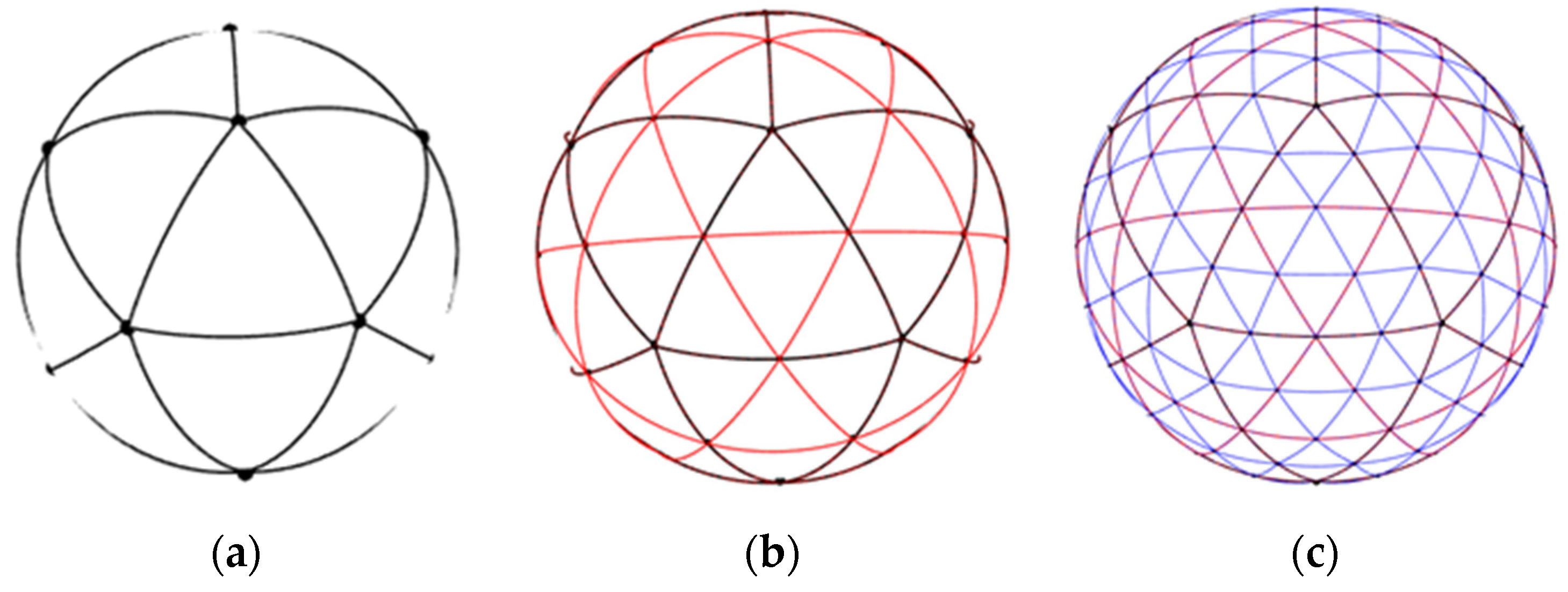
2. Triangle Mesh Generation on a Sphere

Although the SL method belongs to the mesh-free method essentially, it needs a spatial discretization of the spherical surface. In this paper, a triangle mesh based on a regular icosahedron sphere is utilized [18]. As shown in Figure 1, first, a regular icosahedron was embedded in the sphere. To refine this grid, each geodesic edge is split into two equal halves by adding a new vertex at the midpoint, and each triangular face is consequently split into four sub-triangles. Figure 1 illustrates the mesh refinement procedure. The left panel shows a regular icosahedron mapped on the spherical surface, and the middle panel and right panel show the mesh with refinement levels equal to 1 and 2, respectively. Statistically, a triangle mesh which is refined N times will have 10 × 4N +2 vertices and 20 × 4N elements. It is clear that this triangle mesh is semi-structured; there are five triangle elements shared commonly by each of the original twelve vertices on the icosahedron, and each of the reminder grid vertices is shared by six triangles.

3. High-Order Semi-Lagrangian Method

For solving the transport equation, the main idea behind the semi-Lagrangian method is to find the location of the departure point for a grid point and then interpolate to the departure point from the values of its surrounding grid points. As shown in Figure 2, the implementation of the SL method can be divided into the following two procedures:
(1) For each grid point x , integrate the characteristic Equation (4) backward for the location of the departure point x D . Usually the departure point does not coincide with the original node.
d x d t = V ( x , t ) x ( t ) x ( t Δ t ) = t Δ t t V ( x , t ) d t x D = x ( t Δ t ) = x ( t ) t Δ t t V ( x , t ) d t
(2) Then some interpolation method is utilized to interpolate or fit the value on the departure point from those on the original nodes.
ϕ ( x , t ) = ϕ ( x t Δ t t V d t , t Δ t ) = ϕ ( x D , t Δ t ) ϕ t ( x ) = ϕ t Δ t ( x D ) I [ ϕ t Δ t ( x ) ]
where Δ t denotes the discrete time step, I denotes a specific interpolation or fitting operator.
In the following subsections, the above two main procedures would be illustrated, respectively.

3.1. Approximation for Departure Point

In this subsection, two main kinds of methods are utilized to integrate the characteristic Equation (4) for the location of the departure point; those are the Ritchie’s midpoint method and high-order explicit Runge–Kutta methods.

3.1.1. Ritchie’s Method

There are many ways of computing the right-hand integral in Equation (5) approximately, but the most commonly used form has been the midpoint rule, which was first proposed by Ritchie [19] and is iterative and interpolating. Giraldo [20] proved its simplification to the midpoint integration rule on the surface of a sphere. Additionally, the midpoint method was used widespread for the approximation of the characteristic equation in the semi-Lagrangian method [21,22,23]. It is implemented mainly as follows:
Integrate the trajectory equation half of a time step backward, yielding the following:
x M = x M d t 2 V ( x M , t d t / 2 )
where x M enotes the midpoint of the characteristic curve and x A denotes the arrival point. Usually, it was just the mesh vertex. The equation defines a recursive scheme because x M is given implicitly in the relation. Usually, several iterations (4 or 5 iteration loops) are enough to obtain a convergent solution, and then the departure point x D is calculated by the following:
x D = x A d t V ( x M , t d t / 2 )
However, we have said nothing about the order of the interpolations, but obviously, the higher the order of the quadrature formulas, the better the trajectory accuracy, but more computational cost as well. The midpoint rule yields second-order accuracy and has been used quite successfully in 2D planar space. On the sphere, the midpoint rule has to be modified such that the new departure points computed by Equation (8) remain on the surface of the sphere. In other words, after each iteration we must apply the following projection:
x D = R | x D | x D
where R denotes the radius of the sphere.

3.1.2. High-Order Runge–Kutta Methods
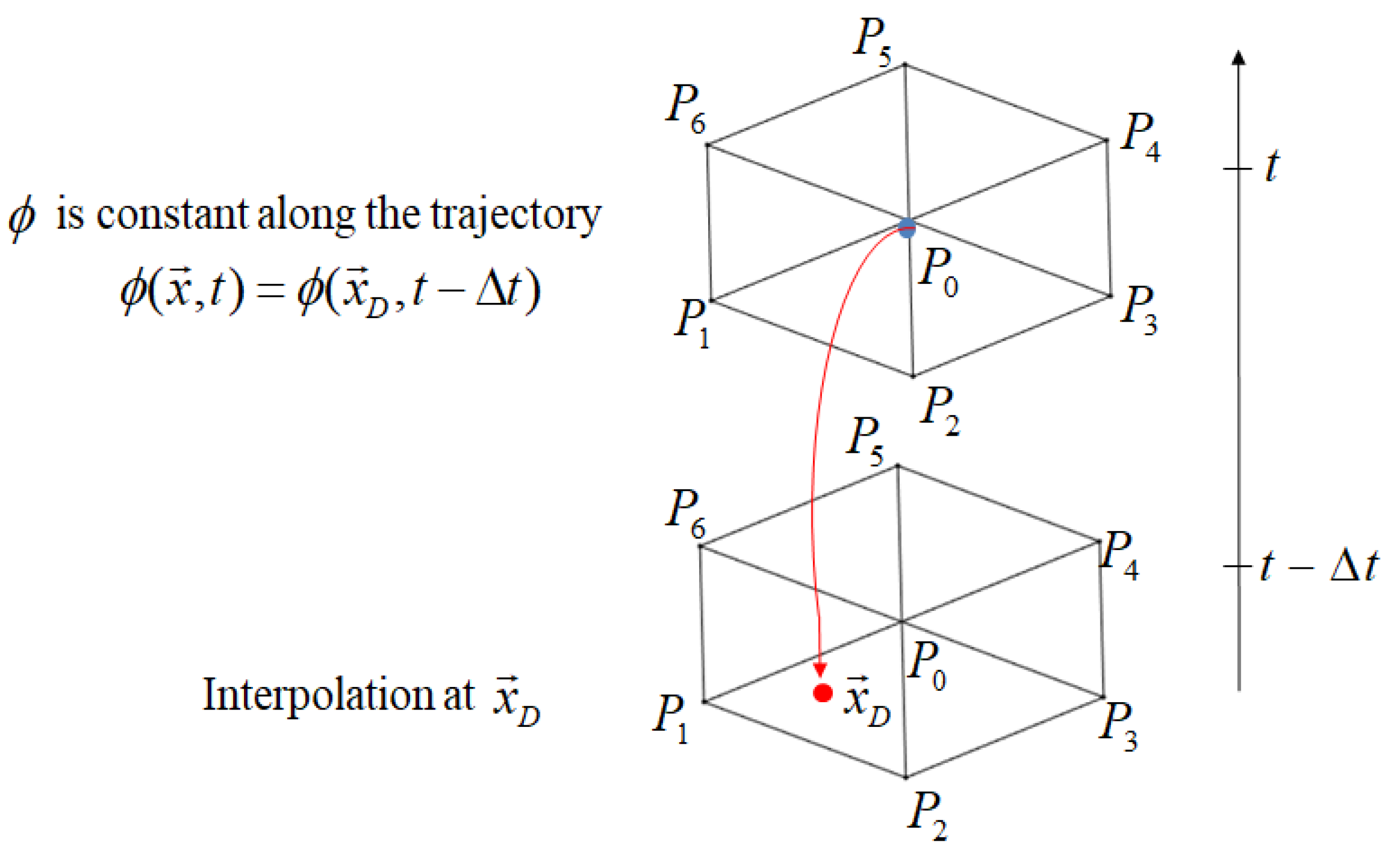
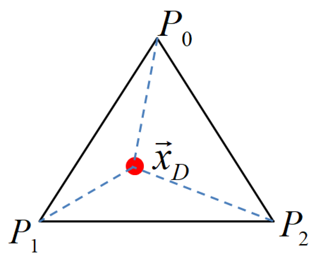
Although the Ritchie’s midpoint method could be implemented easily, it gives only second-order accuracy. Even higher order methods, such as the classical explicit four-order Runge–Kutta method (RK4), could also be used to solve the characteristic equation; it yields the following:
d x k 1 = d t V ( x A , t ) d x k 2 = d t V ( x A + d x k 1 2 , t d t 2 ) d x k 3 = d t V ( x A + d x k 2 2 , t d t 2 ) d x k 4 = d t V ( x A + d x k 3 , t d t ) x D = x A + d x k 1 + 2 d x k 2 + 2 d x k 3 + d x k 4 6
Additionally, classical Butcher’s Runge–Kutta method of order five (RK5) as follows [24]:
d x k 1 = d t V ( x A , t ) d x k 2 = d t V ( x A + d x k 1 4 , t d t 4 ) d x k 3 = d t V ( x A + d x k 1 + d x k 2 8 , t d t 4 ) d x k 4 = d t V ( x A d x k 2 2 d x k 3 2 , t d t 2 ) d x k 5 = d t V ( x A + 3 d x k 1 + 9 d x k 4 16 , t 3 d t 4 ) d x k 6 = d t V ( x A + 3 d x k 1 + 2 d x k 2 + 12 d x k 3 12 d x k 4 + 8 d x k 5 7 , t d t ) x D = x A + ( 7 d x k 1 + 32 d x k 3 + 12 d x k 4 + 32 d x k 5 + 7 d x k 6 ) / 90
When the departure point x D is obtained, then it should be mapped onto the sphere surface by Equation (9). In theory, the high-order Runge–Kutta methods could generate more accurate locations of departure points than the midpoint method. In Section 4, a numerical experiment would be used to validate the results.

3.2. Interpolation

Once the departure point is calculated, then the value at the departure point could be obtained by interpolation or fitting methods. In this section, four methods would be utilized, which include linear interpolation, polynomial fitting based on the least square method, global radial basis function stencil (RBFs), and local RBFs interpolation; the main ideas of these methods would be illustrated, respectively.

3.2.1. Linear Interpolation

The main idea for linear interpolation is as follows. First find the triangle element that the arrival point traced back into, then interpolate its value by those on the triangle’s vertex [25]. For instance, in Figure 3, assuming the red point x D denotes the departure point for a specific vertex and it is located in the triangle element P 0 P 1 P 2 , then its value could be approximated by the values of the three vertexes of the triangle as follows:
ϕ ( x D ) = α 0 ϕ ( P 0 ) + α 1 ϕ ( P 1 ) + α 2 ϕ ( P 2 ) α 0 + α 1 + α 2
where α i , i = 0 , 1 , 2 denotes the spherical area of the sub-triangle formed by the departure point and the edges of the triangle opposite to vertex P i .
This method could be implemented with little effort, and it can be seen that the interpolated value is just an area-weighted average of the values on three vertexes of the triangle.

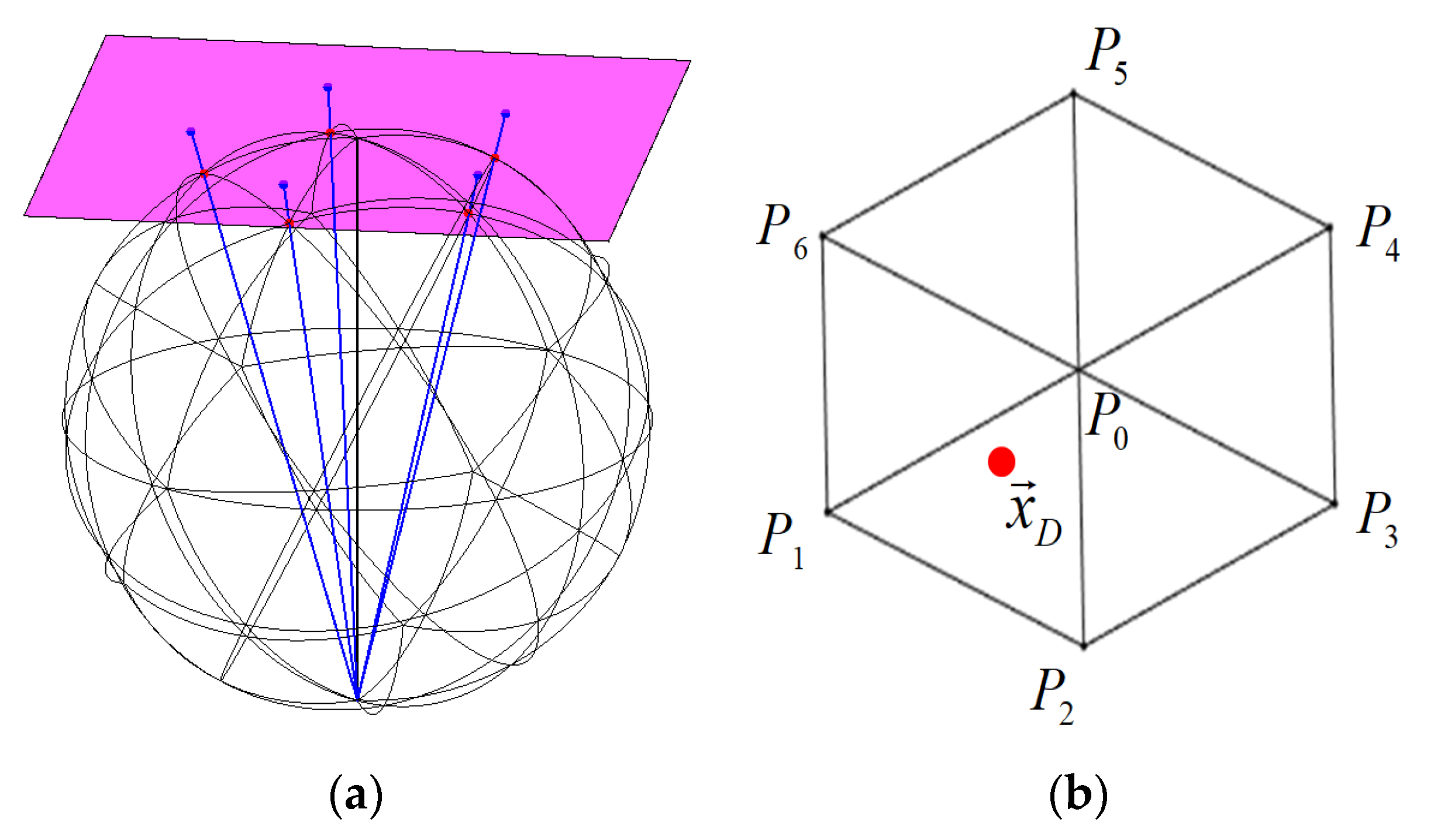
3.2.2. Local Polynomial Fitting by Least-Square Method (Poly-LSQ)

The linear interpolation method above-mentioned has two-order accuracy. In order to attain more accurate interpolation results, high-order polynomial fitting was utilized. It needs a local grid stencil in 3D Cartesian spaces, and then the grid points in this local stencil would be mapped onto a local two-dimensional (2D) coordinate system by a general stereography projection [26,27], and then a bivariate polynomial was utilized to fit the values at grid points on the stencil. In order to obtain an approximate value at the departure point, first, find the nearest vertex for each departure point, and then a polynomial least-squares fit is calculated using values at the vertex and its nearest first-layer neighbor points.
The transformation between the spherical latitude–longitude coordinates and two-dimensional general stereographic coordinates (GSTC) is given by the following:
x = m R cos ( θ ) sin ( λ λ 0 ) y = m R [ sin ( θ ) cos ( θ 0 ) cos ( θ ) sin ( θ 0 ) cos ( λ λ 0 ) ] m = 2 1 + sin ( θ ) sin ( θ 0 ) + cos ( θ ) cos ( θ 0 ) cos ( λ λ 0 )
where m is the map factor and R is the radius of the earth, (   θ , λ ) and (x,y) denote the latitude–longitude coordinates and GSTC respectively. The center of the GSTC is at the tangent point where (x,y) = (0,0). In the transformed system, the positive x-axis is directed toward the east of the origin along the latitudinal circle of θ = θ 0 and the y-axis is defined as positive poleward of the origin along the meridian λ = λ 0 .
In Figure 4a, an icosahedron sphere triangle mesh with refinement level 1 is shown. The north pole and its five nearest neighbor points shown in red dots are projected on the 2D tangent plane, and the blue lines denote projection lines. As shown in Figure 4b, for a specific vertex, its departure point is denoted by the red point x D . Firstly, find the vertex that is closest to this departure point, and then the value at x D could be approximated by the values at the vertex and its first-order neighbor points, which leads to a full bivariate quadratic polynomial as follows:
ϕ ^ ( x , y ) = a 0 + a 1 x + a 2 y + a 3 x 2 + a 4 x y + a 5 y 2
In order to minimize the interpolation error, the fitted polynomial should be constrained by the following condition:
Min i = 1 N B P [ ϕ ^ ( p i ) ϕ ( p i ) ] 2
where the NBP = 6 or 7, is the number of first-order neighbor points for a specific vertex, including the vertex itself. p i denotes the projected point on the local 2D tangent plane.
For Equation (15), there are seven or six values on each stencil but only six polynomial terms. In order to determine the coefficient a i , i = 0 , 1 , , 5 , a Least-squares approach is needed because the system of equations is over-constrained. For a specific vertex, the stencil geometry is expressed in a local coordinate system with the vertex that is nearest the departure point as the origin so that the value at the vertex is equal to the constant coefficient a 0 . Once the coefficients are obtained, an approximate value at the departure point could be obtained by inserting its mapped coordinates into the quadratic polynomial (14).

3.2.3. Global RBFs

In recent two decades, the mesh-free methods have achieved rapid development, among which the radial basis function (RBF) method is one of the most popular numerical methods, and it has been vastly applied to solve various kinds of physical problems with theoretical proofs on solvability and convergence presented in [28]. Increasingly, the global RBF collocation method is applied to some problems in the sphere [29,30].
Given a set of nodes X = { x k } , k = 1 , , N on the sphere surface, the standard global RBF (GRBF) interpolant ϕ ^ ( x ) to the data has the following form:
ϕ ^ ( x ) = k = 1 N ω k B ( x x k )
where B denotes the kernel function of RBF, the notation x = ( x , y , z ) and x k = ( x k , y k , z k ) , the Equation (16) is the linear combination of the kernel function of RBF. In this paper, we will limit our attention to the kernel functions B(r) listed in Table 1. All these four kernel functions are global supported and strictly positive definite. Other types of kernel functions that are local-compactly supported could be found in [31]. Note that there is a parameter c in each kernel function, it is known as the shape parameter.
If the interpolant ϕ ^ ( x ) can be utilized to approximate the true solution, then the expansion coefficients are determine   ω k , k = 1 , , N   by enforcing ϕ ^ ( x k ) = ϕ ( x k ) ,   k = 1 , , N , which can be expressed by the following linear system:
[ B ( x 1 x 1 ) B ( x 1 x 2 ) B ( x 1 x 3 ) B ( x 1 x N ) B ( x 2 x 1 ) B ( x 2 x 2 ) B ( x 2 x 3 ) B ( x 2 x N ) B ( x 3 x 1 ) B ( x 3 x 2 ) B ( x 3 x 3 ) B ( x 3 x N ) B ( x N x 1 ) B ( x N x 2 ) B ( x N x 3 ) B ( x N x N ) ] [ ω 1 ω 2 ω 3 ω N ] = [ ϕ ( x 1 ) ϕ ( x 2 ) ϕ ( x 3 ) ϕ ( x N ) ]
If the Gauss type or IMQ type basis function was used for RBF interpolation, the coefficient matrix in Equation (17) is positive-definite and invertible, and then the linear equations admit a unique solution. If the MQ type basis equation was utilized, the resulting matrix for interpolation may not be positive-definite. Linear-independent polynomial functions can be added to make the matrix positive-definite and invertible. In this case, the RBF interpolant is expressed as follows:
ϕ ^ ( x ) = k = 1 N ω k B ( x x k ) + γ 0 + γ 1 x + γ 2 y + γ 3 z
with the following constraints:
k = 1 N ω k = k = 1 N ω k x k = k = 1 N ω k y k = k = 1 N ω k z k = 0
The resulting linear system:
[ B ( x 1 x 1 ) B ( x 1 x 2 ) B ( x 1 x 3 ) B ( x 1 x N ) 1 x 1 y 1 z 1 B ( x 2 x 1 ) B ( x 2 x 2 ) B ( x 2 x 3 ) B ( x 2 x N ) 1 x 2 y 2 z 2 B ( x 3 x 1 ) B ( x 3 x 2 ) B ( x 3 x 3 ) B ( x 3 x N ) 1 x 3 y 3 z 3 B ( x N x 1 ) B ( x N x 2 ) B ( x N x 3 ) B ( x N x N ) 1 x N y N z N 1 1 1 1 0 0 0 0 x 1 x 2 x 3 x N 0 0 0 0 y 1 y 2 y 3 y N 0 0 0 0 z 1 z 2 z 3 z N 0 0 0 0 ] [ ω 1 ω 2 ω 3 ω N γ 0 γ 1 γ 2 γ 3 ] = [ ϕ ( x 1 ) ϕ ( x 2 ) ϕ ( x 3 ) ϕ ( x N ) 0 0 0 0 ]
The choice of basis function and shape parameter has a significant impact on the accuracy of RBF interpolation. Decreasing c or increasing the number of data points has a severe effect on the stability of the linear system (17) or (20). For a fixed shape parameter c, the condition number of the matrix in the linear system grows exponentially as the number of data points is increased. For a fixed number of data points, as the shape parameter c→0, the basis function becomes increasingly flat; meanwhile, the condition number of the linear system grows exponentially [32]. Figure 5 shows the order of magnitude for the condition number Log10(cond(A)) as a function of shape parameter c under three different mesh refinement levels, where A denotes the coefficient matrix in Equations (17) or (20).
It can be seen that the condition number of the coefficient matrix becomes very large when the value of the shape parameter is close to zero for all four types of basis functions. In general, the condition number of the coefficient matrix grows exponentially as the mesh refinement level increases; the numerical computation tends to become unstable. Meanwhile, the condition number of the coefficient matrix decreased drastically as the value of the shape parameter increased. This is particularly significant because the highest accuracy is often found at some “small” shape parameter, which may result in a large condition number of interpolation matrices and even cause numerical instability. This conflict between accuracy and stability is sometimes referred to as the “trade-off principle”. However, there is no exact analytical formula to obtain the optimal value of the shape parameter. In most cases, it mainly relies on statistical methods [33,34,35,36], such as leave one out cross validation (LOOCV), maximum likelihood estimator (MLE), etc.
One issue with global RBF interpolation is that the coefficient matrix in the linear system is dense, thereby leading to considerable computational costs to solve it directly. Another issue is that the matrices can become ill-conditioned. There are a series of methods to tackle the problem, such as the Contour-Padé, RBF-RA, and RBF-QR algorithms [37]; however, they are not pursued and developed here.

3.2.4. Local RBFs

In order to relieve the problems of ill-conditioning and shape parameter sensitivity of the global RBF, the local RBF method has evolved, and the main idea of the local RBF (LRBF) method applied to the sphere is detailedly presented by [38]. Subsequently, some researchers use LRBF to deal with different complicated problems [39,40,41,42,43,44], etc. Similar to GRBF, LRBF is meshless in character and it needs no polygonization. In contrast to the GRBF, the LRBF is made on the overlapping sub-domains. For approximating the objective function at a given node, only its influence nodes are used. The overlapping sub-domains significantly reduce the size of the linear system at the cost of solving lots of small matrices. In addition, the local RBF method is comparatively less sensitive to the shape parameter. In many cases, the local RBF method can be as accurate as the global RBF method.
For a specific vertex   x i , assuming the node set { x i k } , k = 1 , , n is its n nearest neighbor points including the x i itself ( n N ). The local RBF interpolant ϕ ^ i ( x ) for the vertex x i takes the form:
ϕ ^ i ( x ) = k = 1 n ω i k B ( x x i k )
In the local region influenced by x i , in order to approximate the true solution by the above Equation (21), we could obtain a linear system written in matrix form as follows:
[ B ( x i 1 x i 1 ) B ( x i 1 x i 2 ) B ( x i 1 x i 3 ) B ( x i 1 x i n ) B ( x i 2 x i 1 ) B ( x i 2 x i 2 ) B ( x i 2 x i 3 ) B ( x i 2 x i n ) B ( x i 3 x i 1 ) B ( x i 3 x i 2 ) B ( x i 3 x i 3 ) B ( x i 3 x i n )     B ( x i n x i 1 ) B ( x i n x i 2 ) B ( x i n x i 3 ) B ( x i n x i n ) ] [ ω i 1 ω i 2 ω i 3 ω i n ] = [ ϕ ( x i 1 ) ϕ ( x i 2 ) ϕ ( x i 3 ) ϕ ( x i n ) ]
In the above equation   i 1 , i 2 , , i n , is a vector associated with the center point x i that contains the index of itself and the indices of its n 1 nearest neighboring vertexes, ω i k , k = 1 , , n   is a vector of expansion coefficients.
For a specific departure point, firstly, find the nearest vertex close to it, and then search for the n nearest neighboring vertexes (including the vertex itself) around this vertex. The procedure could be implemented efficiently by the KDtree search method, at last, a corresponding linear system (20) is formed, when the expansion coefficients are obtained, then Equation (19) could be utilized to interpolate the value at the departure point.
The local RBF method suffers from the same problem as the global RBF, yet less severe. Another issue is that there is no exact theory for the optimal size of the local stencil for a specific vertex. Several values are commonly used, such as 31, 50, 74, and 101 are very popular, when the shape parameter of kernel function is fixed, the condition number of the matrix in the linear system grows quickly as the size of local stencil is increased. Therefore, the local stencil size is chosen as 31 in the following numerical test cases if the local RBF method is involved. In Figure 6, a local stencil of size 31 on the icosahedron spherical triangle mesh with refinement level 4 was shown, the center vertex is shown in blue asterisk, and its nearest neighbor points are shown in the red dot.
For the above-mentioned four interpolation methods, the linear interpolation method and the Poly-LSQ method could be implemented without much effort; however, we need to take extra care in selecting the value of the shape parameter in the basis function if the RBF methods are utilized. If no specific explanations, for all the numerical experiments in Section 4 and Section 5, the density of tracer or height fields are placed at the nodes of triangle elements.

4. Trajectory Accuracy and Mass Conservation Evaluation

4.1. Trajectory Accuracy

In a similar manner described in McGregor [45], the accuracy of the trajectories is defined by the following normalized L2 norm:
ϕ ^ i ( x ) = S ( x D x D e x a c t ) 2 d s S ( x D x A ) 2 d s
where x A denotes the arrival point, and x D ,   x D e x a c t denote the calculated departure point and the exact one respectively.   S d s denotes the surface integral on the sphere.
This test case is advection of a Gaussian hill around the sphere [46]. The Gaussian hill is prescribed as follows:
ϕ ^ i = h 0 e b r 2
where r = x x 0 denotes the Euclidean distance between the two points x , x 0 , h 0 = 0.95 and b = 5 respectively. The 3D Cartesian coordinates x = ( x , y , z ) and the latitude–longitude coordinates   ( θ , λ )   on spherical surface are related through
( x , y , z ) = ( R cos θ cos λ , R cos θ sin λ , R sin θ )
where R is the radius of the sphere. The coordinates for the center of the Gaussian distribution x 0 are computed by inserting the tracer center ( θ 0 , λ 0 ) into Equation (25) and evaluating the right-hand side.
The initial wind fields are as follows:
u = u 0 ( cos ( θ ) cos ( α ) + sin ( θ ) cos ( λ π 2 ) sin ( α ) ) V = u 0 sin ( λ π 2 ) sin ( α )
where the flow constant u 0 = 2 π R / ( 64   hours ) , α   is the rotation angular between the wind flow direction and the equatorial plane, the prescribed velocity field is that of solid-body rotation, such that the tracer moves around the earth once with a rotational period of 64 h.
The tracer center was set as ( θ 0 , λ 0 ) = ( 0 , 0 ) , the rotation angle of flow-vectors α = 0 . Then the mid-rule method and high-order Runge–Kutta methods were utilized to solve the trajectory equation for the departure points’ location respectively. The exact location of the test case is given, and comparison of calculated departure points’ location for the midpoint rule method, RK4 and RK5 methods under different time steps are given in Table 2.
It can be seen from Table 2 that when the number of nodes is fixed, as the time step decreased to half of the precedent one, the error of departure points’ location decreased to about 1/4 of the last one; therefore, the midpoint rule method has two-order accuracy. Similarly, it can be seen that the RK4 method achieved four-order accuracy while the RK5 method has at least a five-order convergence rate. Obviously, the RK5 method owns the most accurate results. Therefore, the RK5 method is utilized for computing the location of the departure point in all the following numerical experiments. We also note that an increase in the spatial resolution has little impact on the location errors of departure points when the time step is fixed.

4.2. Mass Conservations

In order to check the conservation of the presented scheme, the mass conservations is commonly used, that is, the total mass should be kept as a constant as follows:
Mass :   I 1 ( t ) = S 2 ϕ ( x , t ) d s d I 1 ( t ) d t = 0
where S 2 ϕ ( x , t ) d s denotes the integral of ϕ on the spherical surface S2. The numerical relative error for   I 1 ( t ) is reported using the following:
( I 1 ( t ) I 1 ( 0 ) ) / I 1 ( t )
In order to facilitate comparison between different methods for the following test case simulations, the L1, L2 and L   norms of mass error are specified as follows [47]:
L 1 = S | ϕ n ( j ) ϕ r ( j ) | d s S | ϕ r ( j ) | d s | ϕ n ( j ) ϕ r ( j ) | A j | ϕ r ( j ) | A j L 2 = S ( ϕ n ( j ) ϕ r ( j ) ) 2 d s S ϕ r ( j ) 2 d s ( ϕ n ( j ) ϕ r ( j ) ) 2 A j ϕ r ( j ) 2 A j L = Max j | ϕ n ( j ) ϕ r ( j ) | Max j | ϕ r ( j ) |
The function ϕ n ( j ) denotes the numerical solution defined at the x j positions on the numerical mesh. The index j represents the specific cell on the pentagon–hexagon mesh dual to the icosahedron spherical triangle mesh, and A j denotes the spherical area associated with the Voronoi cell controlled by vertex x j . The function ϕ r ( j ) is the reference solution that has been calculated at or interpolated to the same x j positions. The reference solution represents a high-resolution solution that is sufficiently accurate for the computation of the error norms if an analytic solution is not available. The function max j | ϕ | finds the global maximum of the | ϕ | evaluated at the x j positions of the numerical mesh.
In order to test the interpolation accuracy of four different methods and check the mass conservation, the above-mentioned Gauss hill advection is utilized as the benchmark again, and the mesh refinement level is equal to 4. The relative error norm of the tracer calculated by four different methods for interpolation is shown in Figure 7. It can be seen that when the time step is too large, the error norm increases. Obviously, the linear interpolation method gives results with relatively large errors in Figure 7a. If the time step is more than 4 h, the method would generate large errors. In comparison, the polynomial fitting by the least-square method could generate more accurate results, as shown in Figure 7b. With an appropriate value of shape parameter, the global RBF and local RBF could also give more accurate results in Figure 7c,d, for the global RBF method, the Gauss basis function is utilized, and the shape parameter c =1.5; for the local RBF method, the Gauss basis function is utilized, the size of the local stencil is 31, and the shape parameter c = 1.5. It is obvious the last three methods generate results that are in the same order of magnitude. We also note that the global RBF and local RBF methods give much like results.

5. Numerical Experiments

In this section, the semi-Lagrangian method will be utilized to model the evolution process of the advection of a passive tracer; three test cases are considered. They are referred to as the solid body rotation, the shear deformation of twin slotted cylinders, and the moving vortex. In the first case, the mass conservation properties of our scheme would be numerically evaluated. Additionally, the modeling results would be presented in the other two cases.
Test case 1: solid body rotation
This test case describes the advection of a cosine bell once around the sphere [48,49,50]. The initial shape of the bell is formulated as follows:
ϕ = { h 0 2 ( 1 + cos π r R b ) ,                                                                                     i f   r < R b                               0 ,                                                                                                                   i f   r R b                            
where   h 0 = 1000   m   denotes the initial bell maximize height. R b = R / 3 is the radius of the cosine bell,     r denotes the great circle distance between ( λ , θ ) and the center of the cosine bell ( λ 0 , θ 0 ) = ( 0 , 0 ) , given by the following:
r = R cos 1 ( sin ( θ ) sin ( θ 0 ) + cos ( θ ) cos ( θ 0 ) cos ( λ λ 0 ) )
The numerical results of the SL scheme are implemented on Tri_Icosa_L5 mesh with the time step equal to 12 hours (h). The initial wind fields are the same as Equation (26), while the parameter u 0 = 2 π R / ( 12   days ) , days = 24 h.
To check the influence of the wind flow direction α upon the icosahedron sphere gird, this test is conducted with α = 0 (eastward along the equator) and α = π / 2 (across the north and south poles) respectively. In Figure 8a, it shows L1, L2, and L   norm error for the cosine bell test case by the global RBF method with Gauss kernel function; the shape parameter is 16, and the wind direction angle α = 0 ; Figure 8b shows the same content but the wind direction angle   α = π / 2 . In Figure 8c, it shows L1, L2 and L   norm error for the cosine bell test case by the local RBF method with Gauss kernel function; the shape parameter is 20, the wind direction angle α = 0 ; Figure 8d shows the same content but the wind direction angle   α = π / 2 . It can be seen that the history of normalized errors of mass by the local RBF method with different flow angles is almost the same; four panels show the L1, L2 error norms are in the same order of magnitude, which means that the wind direction angle has little effect on the total mass. This accords with the facts. We also note that the normalized errors by the global RBF method are slightly more accurate than those by the local RBF method.
In order to evaluate the efficiency of the proposed SL method, another three methods for the approximation of the transport equation on the sphere were utilized for comparison, those are, the RBF method, pseudo-spectral method (PS), and two-order finite difference (FD2) method [51]. The SL method and RBF method are implemented on an icosahedron sphere triangle mesh and the Gauss basis function is used. The PS method and FD2 method are on latitude–longitude grids. The explicit four-order classical Runge–Kutta method was used in all methods for time integration except the SL method. Table 3 shows the comparison results of mass error between the proposed SL method, the PS method, the FD2 method, and the RBF method under different spatial resolutions.
From the L 2 and L norm of mass error shown in Table 3, it can be seen that the results obtained by the SL method based on global RBF interpolation own the most accuracy, and then the RBF method follows; at last, the PS method and FD2 method give least accurate results. It could also be noted that the SL method admits a relatively larger time step than other methods.
Test case 2: Deformation of twin slotted cylinders
In this test case, the tracer’s shape is not smooth, and it is more challenging and designed to assess the shape-preserving properties of the proposed method, the tracer has a distribution shape of twin slotted cylinders defined as follows [52,53,54]:
ϕ ( λ , θ , t ) | t = 0 = { 1 , i f   r i R b   a n d   | λ λ i | R b 6   f o r   i = 0 , 1 1 , i f   r 0 R b   a n d   | λ λ 0 | < R b 6   a n d   θ θ 0 < 5 R b 12 1 , i f   r 1 R b   a n d   | λ λ 1 | < R b 6   a n d   θ θ 1 > 5 R b 12 0 , o t h e r w i s e
where R b denotes the radius of the cylinder,   R b = 0.5 . r i = r i ( λ , θ ) is the great-circle distance from the center of the cylinder located at ( λ i , θ i ) , i = 0 , 1 . The initial positions of the centers of two cylinders are at ( λ 0 , θ 0 ) = ( π 6 , 0 ) and   ( λ 1 , θ 1 ) = ( π 6 , 0 )   respectively. The slots are oriented in opposite directions for the two cylinders so that they are symmetric with respect to the flow.
The wind field is non-divergent but highly deformational. The initial distributions are deformed into thin filaments halfway through the simulation while they are being transported along the zonal direction by the solid-body component of the flow. Note that an exact solution for this test is only available at the final time t = T, and it is just the same as the initial distributions. The time-dependent non-divergent wind field is defined as follows:
u ( λ , θ , t ) = κ sin 2 ( λ ^ ) sin ( 2 θ ) cos ( π t / T ) + 2 π cos ( θ ) / T V ( λ , θ , t ) = κ sin ( 2 λ ^ ) cos ( θ ) cos ( π t / T )
where λ ^ = λ 2 π t T , κ = 2.0 , and the final time T = 5 in non-dimensional time units.
An icosahedron sphere triangle mesh with refinement level 5 is used. The initial distribution of the tracer is shown in Figure 9a, and Figure 9b shows the tracer’s restoration to the original shape at the final time by the Poly-LSQ method with   Δ t = 0.1 . Figure 9c shows the tracer’s shape at the final time by the global RBF interpolation based on the Gauss kernel function with shape parameter c = 18.0, time step   Δ t = 0.1 ; Figure 9d shows the tracer’s shape at the final time by the local RBF method based on the Gauss kernel function with shape parameter c = 19.0, time step   Δ t = 0.1 .
It can be seen that the above three interpolation methods could reproduce this complicated deformational flow correctly, while the shape edges of the twin cylinders are smeared, and small overshoots or undershoots are observed near the sharp edges of the twin cylinders. For the Poly-LSQ method and the local RBF method, the oscillations are more obvious in the upwind direction near the edge of the twin cylinders than in the global RBF method. In general, the global RBF method performs the best.
Test case 3: moving vortex
In order to further test the advection scheme representing tracer evolution in a non-divergent but deforming flow, this test case is about the evolution of idealized cyclogenesis on the sphere, which was first described by Nair et al. [55], and then was used as a benchmark for transport processes on a spherical surface. The initial condition was spun up by an angular velocity field, resulting in two diametrically opposed vortices. Let ( λ ´ , θ ´ ) be the rotated coordinate system with the north pole at ( λ p , θ p ) with respect to the regular spherical coordinates   ( λ , θ ) . It follows:
λ ´ = tan 2 1 ( sin ( λ λ p ) , sin ( θ p ) cos ( λ λ p ) cos ( θ p ) tan ( θ ) ) θ ´ = sin 1 ( sin ( θ ) sin ( θ p ) + cos ( θ ) cos ( θ p ) cos ( λ λ p ) )
The wind fields are a combination of wind vectors of the solid rotation and that of the deformational flow, which are specified as follows:
u = u 0 ( cos ( θ ) cos ( α ) + cos ( λ ) sin ( θ ) sin ( α ) ) + ω ( θ ´ ) [ sin ( θ c ( t ) ) cos ( θ ) cos ( θ c ( t ) ) cos ( λ λ c ( t ) ) sin ( θ ) ] V = u 0 sin ( λ ) sin ( α ) + ω ( θ ´ ) [ cos ( θ c ( t ) ) sin ( λ λ c ( t ) ) ]
where ( λ c ( t ) , θ c ( t ) ) denotes the center of the vortex, which is free to move anywhere on the sphere. The scaled tangential velocity is as follows:
ω ( θ ´ ) = { u 0 3 3 2 ρ ( θ ´ ) sec h 2 ( ρ ( θ ´ ) ) tanh ( ρ ( θ ´ ) )                             i f   ρ ( θ ´ ) 0 0                                                                                                                                                   i f   ρ ( θ ´ ) = 0                            
where ρ ( θ ´ ) = ρ 0 cos ( θ ´ ) is the radial distance of the vortex. The background flow constant u 0 = 2 π R / ( 12   days ) . The exact solution in non- dimensional units at time t is given by the following:
  ϕ ( λ ´ , θ ´ , 0 ) = 1 tan h ( ρ ( θ ´ ) γ sin ( λ ´ ω ( θ ´ ) t ) )
where γ   is a parameter defining the characteristic width of the frontal zone. We set ρ 0 = 3 and γ = 5 .With these parameters, the initial condition ϕ ( λ ´ , θ ´ , 0 )   is displayed in Figure 10a.
In this case, an icosahedron sphere triangle mesh with refinement level 5 is used, global RBF interpolation based on the Gauss kernel function was implemented and shape parameter c = 16, time step   Δ t = 0.5 h. Initially a vortex center is located at the following:
( λ c ( t ) , θ c ( t ) ) | t = 0 = ( π 2 , 0 )
with this setup the other vortex center will be placed at the diametrically opposite point ( π 2 , 0 ) . Thus the vortices have the initial and final positions (after one complete revolution) geographically located at 90° E and 90° W on the equator, as shown in Figure 10b,c.
In Figure 10c, it can be seen that a couple of vortices with correct rotation structures are evolving and there are no obvious oscillations around large gradients. The proposed scheme can simulate this complicated procedure successfully.

6. Conclusions

A computationally efficient and high-order backward trajectory semi-Lagrangian approach has been proposed for the solution of the transport equation on the sphere. We test several kinds of interpolation methods for the values at departure points.
The main conclusions are as follows:
(1)
Although the semi-Lagrangian method is not constrained by the CFL number, the time step for backward integration could not be too large arbitrarily, especially for flows of complex structures;
(2)
A high-order explicit integration method could be utilized to solve the characteristic equation in order to obtain more accurate locations of departure points. The SL method does not guarantee mass conservation; however, the mass is conserved well in test cases for numerical experiments when the solution is smooth;
(3)
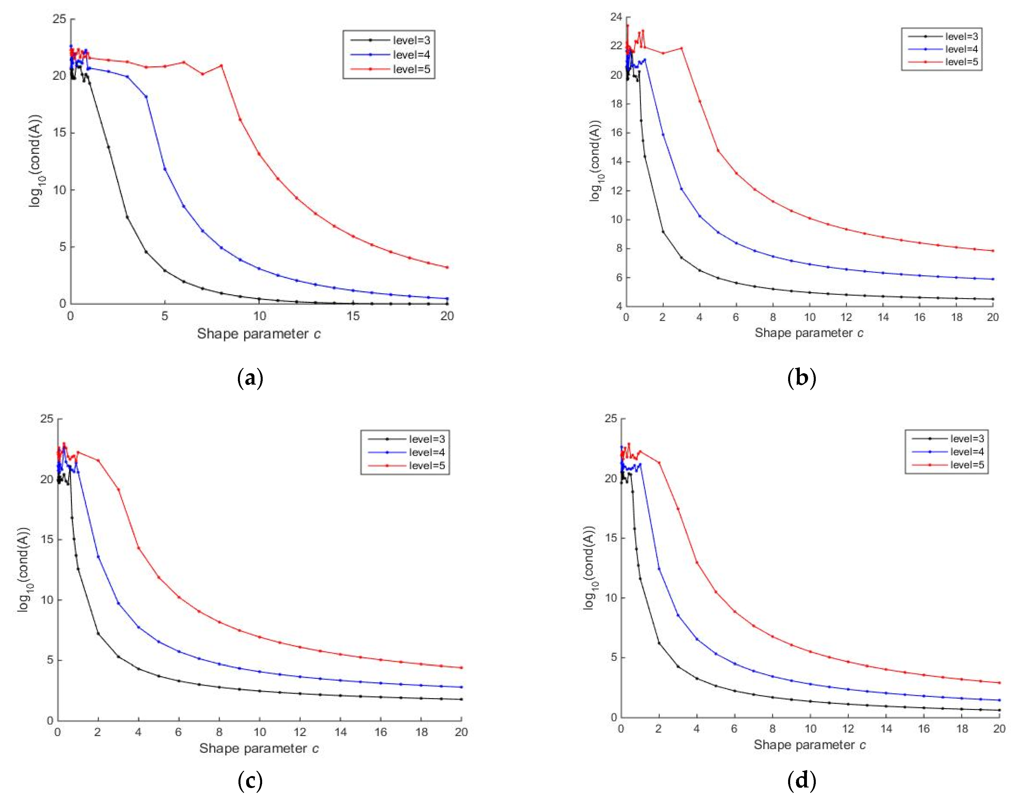
Among different interpolation methods, results obtained by the linear interpolation method show too much diffusion, especially in the great gradient region of the solution. Compared to linear interpolation, more accurate results could be obtained by the Poly-LSQ method and the global or local RBF interpolation method. However, the value of the shape parameter for the basic function is key to the RBF interpolation. AN inappropriate value would cause a great loss of accuracy in the interpolation results, even numerical instability. It costs a lot of effort to select an optimal value. While this problem does not occur for the linear and Poly-LSQ methods. When the solution is not smooth, it tends to generate small ripples in the steep gradient region of the solution if the Poly-LSQ method, global RBFs, or local RBFs would be utilized. Therefore, the techniques to suppress numerical oscillations should be developed in further research;
(4)
Essentially, the proposed SL method is meshless and implemented in 3D Cartesian coordinates; it could be extended to other kinds of grids on the sphere directly.

Author Contributions

Conceptualization, F.L. and F.Z.; methodology, F.L.; software, T.W.; validation, F.L.; formal analysis, F.L.; investigation, F.L.; resources, F.L. and F.Z.; validation, F.L.; visualization, G.T. and F.W.; writing—original draft, F.L.; writing—review and editing, F.L. and F.Z. All authors have read and agreed to the published version of the manuscript.

Funding

This research was financially supported by the National Natural Science Foundation of China (Grant no. 41901323, Grant no. 61875022), the Jiangsu Province “333” project (Grant no. BRA2020152).

Institutional Review Board Statement

Not applicable.

Informed Consent Statement

Not applicable.

Data Availability Statement

The data are available from the corresponding author on reasonable request.

Conflicts of Interest

The authors declare no conflict of interest.

References

  1. Chen, M.; Lv, G.; Zhou, C.; Lin, H.; Ma, Z.; Yue, S.; Wen, Y.; Zhang, F.; Wang, J.; Zhu, Z.; et al. Geographic modeling and simulation systems for geographic research in the new era: Some thoughts on their development and construction. Sci. China Earth Sci. 2021, 64, 1207–1223. [Google Scholar] [CrossRef]
  2. Chen, M.; Voinov, A.; Ames, D.P.; Kettner, A.J.; Goodall, J.L.; Jakeman, A.J.; Barton, M.C.; Harpham, Q.; Cuddy, S.M.; DeLuca, C.; et al. Position paper: Open web-distributed integrated geographic modelling and simulation to enable broader participation and applications. Earth-Sci. Rev. 2020, 207, 103223. [Google Scholar] [CrossRef]
  3. Lü, G.; Batty, M.; Strobl, J.; Lin, H.; Zhu, A.-X.; Chen, M. Reflections and speculations on the progress in Geographic Information Systems (GIS): A geographic perspective. Int. J. Geogr. Inf. Sci. 2019, 33, 346–367. [Google Scholar] [CrossRef] [Green Version]
  4. Prusa, J.M. Computation at a coordinate singularity. J. Comput. Phys. 2018, 361, 331–352. [Google Scholar] [CrossRef]
  5. Tang, J.; Chen, C.; Shen, X.; Xiao, F.; Li, X. A Positivity-preserving Conservative Semi-Lagrangian Multi-moment Global Transport Model on the Cubed Sphere. Adv. Atmos. Sci. 2021, 38, 1460–1473. [Google Scholar] [CrossRef]
  6. Staniforth, A.; Thuburn, J. Horizontal grids for global weather and climate prediction models: A review. Q. J. R. Meteorol. Soc. 2012, 138, 1–26. [Google Scholar] [CrossRef]
  7. Chen, M.; Lü, G.N.; Lu, F.Q.; Wan, G. Grid systems for geographic modelling and simulation: A review. Sci. Found. China 2018, 26, 47–68. [Google Scholar]
  8. Zerroukat, M.; Allen, T. On the monotonic and conservative transport on overset/Yin–Yang grids. J. Comput. Phys. 2015, 302, 285–299. [Google Scholar] [CrossRef]
  9. Ivan, L.; De Sterck, H.; Susanto, A.; Groth, C. High-order central ENO finite-volume scheme for hyperbolic conservation laws on three-dimensional cubed-sphere grids. J. Comput. Phys. 2015, 282, 157–182. [Google Scholar] [CrossRef]
  10. Giorgetta, M.A.; Brokopf, R.; Crueger, T.; Esch, M.; Fiedler, S.; Helmert, J.; Hohenegger, C.; Kornblueh, L.; Köhler, M.; Manzini, E.; et al. ICON-A, the Atmosphere Component of the ICON Earth System Model: I. Model Description. J. Adv. Model. Earth Syst. 2018, 10, 1613–1637. [Google Scholar] [CrossRef]
  11. Logemann, K.; Linardakis, L.; Korn, P.; Schrum, C. Global tide simulations with ICON-O: Testing the model performance on highly irregular meshes. Ocean Dyn. 2021, 71, 43–57. [Google Scholar] [CrossRef]
  12. Miura, H.; Skamarock, W.C. An Upwind-Biased Transport Scheme Using a Quadratic Reconstruction on Spherical Icosahedral Grids. Mon. Weather Rev. 2013, 141, 832–847. [Google Scholar] [CrossRef] [Green Version]
  13. Dubey, S.; Dubos, T.; Hourdin, F.; Upadhyaya, H. On the inter-comparison of two tracer transport schemes on icosahedral grids. Appl. Math. Model. 2015, 39, 4828–4847. [Google Scholar] [CrossRef]
  14. Diamantakis, M. The Semi-Lagrangian Technique in Atmospheric Modelling: Current Status and Future Challenges. In Proceedings of the ECMWF Seminar in Numerical Methods for Atmosphere and Ocean Modelling, Reading, UK, 2–5 September 2013; pp. 183–200. [Google Scholar]
  15. Harris, L. A New Semi-Lagrangian Finite Volume Advection Scheme Combines the Best of Both Worlds. Adv. Atmos. Sci. 2021, 38, 1608–1609. [Google Scholar] [CrossRef]
  16. Fletcher, S.J. Semi-Lagrangian Advection Methods and Their Applications in Geoscience; Elsevier: Amsterdam, The Netherlands, 2019. [Google Scholar]
  17. Mittal, R.; Upadhyaya, H.C.; Sharma, O.P. On Near-Diffusion-Free Advection over Spherical Geodesic Grids. Mon. Weather Rev. 2007, 135, 4214–4225. [Google Scholar] [CrossRef]
  18. Subich, C.J. Higher-order finite volume differential operators with selective upwinding on the icosahedral spherical grid. J. Comput. Phys. 2018, 368, 21–46. [Google Scholar] [CrossRef]
  19. Ritchie, H. Semi-Lagrangian Advection on a Gaussian Grid. Mon. Weather Rev. 1987, 115, 608–619. [Google Scholar] [CrossRef]
  20. Giraldo, F.X. Trajectory Calculations for Spherical Geodesic Grids in Cartesian Space. Mon. Weather Rev. 1999, 127, 1651–1662. [Google Scholar] [CrossRef]
  21. Carfora, M.F. Semi-Lagrangian advection on a spherical geodesic grid. Int. J. Numer. Methods Fluids 2007, 55, 127–142. [Google Scholar] [CrossRef]
  22. Varun, S.; Wright, G.B. Mesh-free Semi-Lagrangian methods for transport on a sphere using radial basis functions. J. Comput. Phys. 2018, 366, 170–190. [Google Scholar]
  23. Diamantakis, M.; Filip, V. A fast converging and concise algorithm for computing the departure points in Semi-Lagrangian weather and climate models. J. R. Meteorol. Soc. 2022, 148, 670–684. [Google Scholar] [CrossRef]
  24. Hossain, B.; Hossain, J.; Miah, M.; Alam, S. A comparative study on fourth order and Butcher’s fifth order Runge-Kutta methods with third order initial value problem (IVP). Appl. Comput. Math. 2017, 6, 243–253. [Google Scholar] [CrossRef]
  25. Tomitaa, H.; Tsugawaa, M.; Satoha, M.; Gotob, K. Shallow Water Model on a Modified Icosahedral Geodesic Grid by Using Spring Dynamics. J. Comput. Phys. 2001, 174, 579–613. [Google Scholar] [CrossRef]
  26. Lee, J.-L.; MacDonald, A.E. A Finite-Volume Icosahedral Shallow-Water Model on a Local Coordinate. Mon. Weather Rev. 2009, 137, 1422–1437. [Google Scholar] [CrossRef]
  27. Dubey, S.; Mittal, R.; Lauritzen, P.H. A flux-form conservative semi-Lagrangian multitracer transport scheme (FF-CSLAM) for icosahedral-hexagonal grids. J. Adv. Model. Earth Syst. 2014, 6, 332–356. [Google Scholar] [CrossRef]
  28. Fasshauer, G.E. Meshfree Approximation Methods with MATLAB; World Scientific Publishing Co Pte. Ltd.: Singapore, 2007. [Google Scholar]
  29. Flyer, N.; Wright, G.B. Transport schemes on a sphere using radial basis functions. J. Comput. Phys. 2007, 226, 1059–1084. [Google Scholar] [CrossRef] [Green Version]
  30. Flyer, N.; Lehto, E. Rotational transport on a sphere: Local node refinement with radial basis functions. J. Comput. Phys. 2010, 229, 1954–1969. [Google Scholar] [CrossRef]
  31. Parand, K.; Hemami, M. Numerical Study of Astrophysics Equations by Meshless Collocation Method Based on Compactly Supported Radial Basis Function. Int. J. Appl. Comput. Math. 2017, 3, 1053–1075. [Google Scholar] [CrossRef] [Green Version]
  32. Afiatdoust, F.; Esmaeilbeigi, M. Optimal variable shape parameters using genetic algorithm for radial basis function approximation. Ain Shams Eng. J. 2015, 6, 639–647. [Google Scholar] [CrossRef]
  33. Fasshauer, G.E.; Zhang, J.G. On choosing “optimal” shape parameters for RBF approximation. Numer. Algorithms 2007, 45, 345–368. [Google Scholar] [CrossRef]
  34. Uddin, M. On the selection of a good value of shape parameter in solving time-dependent partial differential equations using RBF approximation method. Appl. Math. Model. 2014, 38, 135–144. [Google Scholar] [CrossRef]
  35. Mongillo, M. Illinois Institute of Technology Choosing Basis Functions and Shape Parameters for Radial Basis Function Methods. SIAM Undergrad. Res. Online 2011, 4, 190–209. [Google Scholar] [CrossRef]
  36. Cavoretto, R.; De Rossi, A.; Mukhametzhanov, M.S.; Sergeyev, Y.D. On the search of the shape parameter in radial basis functions using univariate global optimization methods. J. Glob. Optim. 2021, 79, 305–327. [Google Scholar] [CrossRef]
  37. Wright, G.B.; Fornberg, B. Stable computations with flat radial basis functions using vector-valued rational approximations. J. Comput. Phys. 2017, 331, 137–156. [Google Scholar] [CrossRef] [Green Version]
  38. Flyer, N.; Wright, G.B.; Fornberg, B. Radial Basis Function-generated Finite Differences: A Mesh-free Method for Computational Geosciences. In Handbook of Geomathematics; Freeden, W., Nashed, M., Sonar, T., Eds.; Springer: Berlin/Heidelberg, Germany, 2013. [Google Scholar]
  39. Yao, G.; Duo, J.; Chen, C.; Shen, L. Implicit local radial basis function interpolations based on function values. Appl. Math. Comput. 2015, 265, 91–102. [Google Scholar] [CrossRef]
  40. Ahmad, I.; Khaliq, A. Local RBF method for multi-dimensional partial differential equations. Comput. Math. Appl. 2017, 74, 292–324. [Google Scholar] [CrossRef]
  41. Sun, J.; Yi, H.-L.; Xie, M.; Tan, H.-P. New implementation of local RBF meshless scheme for radiative heat transfer in participating media. Int. J. Heat Mass Transf. 2016, 95, 440–452. [Google Scholar] [CrossRef]
  42. Oru, M. Two meshless methods based on local radial basis function and barycentric rational interpolation for solving 2D viscoelastic wave equation. Comput. Math. Appl. 2020, 79, 3272–3288. [Google Scholar]
  43. Gunderman, D.; Flyer, N.; Fornberg, B. Transport schemes in spherical geometries using spline-based RBF-FD with polynomials. J. Comput. Phys. 2020, 408, 109256. [Google Scholar] [CrossRef]
  44. Flyer, N.; Fornberg, B.; Bayona, V.; Barnett, G.A. On the role of polynomials in RBF-FD approximations: I. Interpolation and accuracy. J. Comput. Phys. 2016, 321, 21–38. [Google Scholar] [CrossRef] [Green Version]
  45. McGregor, J.L. Economical Determination of Departure Points for Semi-Lagrangian Models. Mon. Weather Rev. 1993, 121, 221–230. [Google Scholar] [CrossRef]
  46. Lauritzen, P.H.; Skamarock, W.C.; Prather, M.J.; Taylor, M.A. A standard test case suite for two-dimensional linear transport on the sphere. Geosci. Model Dev. 2012, 5, 887–901. [Google Scholar] [CrossRef] [Green Version]
  47. Ringler, T.; Thuburn, J.; Klemp, J.; Skamarock, W. A unified approach to energy conservation and potential vorticity dynamics for arbitrarily-structured C-grids. J. Comput. Phys. 2010, 229, 3065–3090. [Google Scholar] [CrossRef]
  48. Gavete, L.; Alonso, B.; Ureña, F.; Benito, J.J.; Herranz, J. Pseudo-spectral/finite-difference adaptive method for spherical shallow-water equations. Int. J. Comput. Math. 2008, 85, 461–473. [Google Scholar] [CrossRef]
  49. Williamson, D.L.; Drake, J.B.; Hack, J.J.; Jakob, R.; Swarztrauber, P.N. A standard test set for numerical approximations to the shallow water equations in spherical geometry. J. Comput. Phys. 1992, 102, 211–224. [Google Scholar] [CrossRef]
  50. Mohammadi, V.; Dehghan, M.; Khodadadian, A.; Wick, T. Numerical investigation on the transport equation in spherical coordinates via generalized moving least squares and moving kriging least squares approximations. Eng. Comput. 2021, 37, 1231–1249. [Google Scholar] [CrossRef]
  51. Fornberg, B.; Merrill, D. Comparison of finite difference- and pseudospectral methods for convective flow over a sphere. Geophys. Res. Lett. 1997, 24, 3245–3248. [Google Scholar] [CrossRef] [Green Version]
  52. Zhang, Y.; Yu, R.; Li, J. Implementation of a conservative two-step shape-preserving advection scheme on a spherical icosahedral hexagonal geodesic grid. Adv. Atmos. Sci. 2017, 34, 411–427. [Google Scholar] [CrossRef]
  53. Zhang, Y.; Nair, R.D. A Nonoscillatory Discontinuous Galerkin Transport Scheme on the Cubed Sphere. Mon. Weather Rev. 2012, 140, 3106–3126. [Google Scholar] [CrossRef] [Green Version]
  54. Dong, L.; Wang, B. Trajectory-Tracking Scheme in Lagrangian Form for Solving Linear Advection Problems: Interface Spatial Discretization. Mon. Weather Rev. 2013, 141, 324–339. [Google Scholar] [CrossRef]
  55. Nair, R.D.; Jablonowski, C. Moving Vortices on the Sphere: A Test Case for Horizontal Advection Problems. Mon. Weather Rev. 2008, 136, 699–711. [Google Scholar] [CrossRef]
Figure 1. The triangle mesh based on a regular icosahedron sphere. (a)The initial triangle mesh generated by regular icosahedron embedded in the sphere, with edges projected to the surface; (b) icosahedron triangle mesh with refinement level 1, with newly added edges denoted via thinner red lines; (c) icosahedron triangle mesh after two stages of refinement, newly added edges are shown in blue lines.
Atmosphere 13 01807 g001
Figure 2. The main idea of a SL method. For a specific vertex P0 , its departure point is denoted by x D , the red curve denotes a characteristic curve. The value at arrival point P0 at current time level just originates from the value at its departure point at the previous time level.
Atmosphere 13 01807 g002
Figure 3. Linear interpolation at the departure point, its value is approximated by the values on three vertexes of the triangle.
Atmosphere 13 01807 g003
Figure 4. General stereography projection on a local stencil on the icosahedron sphere (a) icosahedron spherical triangle mesh with refinement level 1, the stereographic projection of north pole, and its nearest five neighbor points are shown in red dot, the mapped points are shown in blue dot on the local 2D tangent plane shown in pink; (b) the first-order neighbor points for a specific vertex. The number of first-order neighbor points around each vertex is 6 (except for the 12 original major points, the number of first-order neighbor points around is 5).
Atmosphere 13 01807 g004
Figure 5. Log10cond(A) as a function of shape parameter c (a) when global RBF based on Gauss basis function is utilized for interpolation; (b) when global RBF based on MQ basis function is utilized for interpolation; (c) when global RBF based on IMQ basis function is utilized for interpolation; (d) when global RBF based on IQ basis function is utilized for interpolation.
Atmosphere 13 01807 g005
Figure 6. A local stencil of size 31 on the icosahedron spherical triangle mesh with refinement level 4. The center vertex is shown in blue asterisk and its nearest neighbor points are shown in red dot.
Atmosphere 13 01807 g006
Figure 7. The history of mass relative error on icosahedron sphere grids with refinement level 4. Advection of the height field is eastward along the equator by SL method for different interpolation methods (a) Linear interpolation; (b) Poly-LSQ; (c) global RBFs; (d) local RBFs.
Atmosphere 13 01807 g007
Figure 8. The L1, L2 and L norm error for the cosine bell test case as a function of time on the icosahedron sphere triangle mesh with refinement level 5, Advection of the height field around the sphere once. Results are for the global RBF method and local RBF method with dt = 12 h. Gauss kernel function was used. (a) Global RBF and the wind direction angle   α = 0 ; (b) global RBF and the wind direction angle α = π / 2 ; (c) local RBF and the wind direction angle   α = 0 ; (d) local RBF and the wind direction angle   α = π / 2 .
Atmosphere 13 01807 g008
Figure 9. Shear deformation of twin slotted cylinders simulated on icosahedron sphere with refinement level 5. (a) Initial distributions of tracer and (b) The SL numerical solution of the scalar field obtained by Poly-LSQ method at final time t = T, time step Δ t = 0.1 ; (c) The SL numerical solution of the scalar field obtained by global RBF method at final time, time step Δ t = 0.1 ; (d) The SL numerical solution of the scalar field obtained by local RBF method at final time, time step   Δ t = 0.1 .
Atmosphere 13 01807 g009aAtmosphere 13 01807 g009b
Figure 10. Moving vortex (a) initial scalar field and (b) analytic solution after 12 days for the moving vortex problem. The centers of the vortices are located on the equator at 90° E initially and at 90° W after 12 days. (c) The SL numerical solution of the scalar field after one full revolution (12 days). The SL advection scheme employs global RBF method on the icosahedron sphere mesh with refinement level 5 and the wind direction angle   α = 0 ,     Δ t = 0.5 , hour.
Atmosphere 13 01807 g010
Table 1. Definitions of some infinitely differentiable radial functions, the shape parameter c controls their flatness.
Name of RBFAbbreviationDefinition
GaussianGA e ( c r ) 2
MultiquadricMQ 1 + ( c r ) 2
Inverse multiquadricIMQ 1 1 + ( c r ) 2
Inverse quadraticIQ 1 1 + ( c r ) 2
Table 2. The comparison for departure points’ location error between exact solution and these of three different methods.
Refinement LevelNode NumberTime-StepMidpoint RuleRK4RK5
Level 36422 h0.0012 5.4257 × 10 6 2.3382 × 10 8
4 h0.0049 8.6429 × 10 5 8.1214 × 10 7
8 h0.02051.4 × 10−3 3.2846 × 10 5
Level 425622 h0.0012 5.4263 × 10 6 2.3368 × 10 8
4 h0.0049 8.6440 × 10 5 8.1174 × 10 7
8 h0.02051.4 × 10−3 3.2840 × 10 5
Level 510,2422 h0.0012 5.4264 × 10 6 2.3364 × 10 8
4 h0.0049 8.6442 × 10 5 8.1164 × 10 7
8 h0.02051.4 × 10−3 3.2838 × 10 5
Table 3. Comparison results between the proposed SL method, the PS method, FD2 method, and RBF method under different space resolutions.
MethodBasis Function and cNode NumberTime-Step L 2 Norm L Norm
SL method (Global RBFs) GA, c = 1.56424 h0.04430.0371
GA, c = 6.025622 h0.00460.0030
GA, c = 16.010,2421 h0.00110.0011
PS method- 32 × 16 9/40 h0.22430.1874
- 64 × 32 9/80 h0.05580.0460
- 128 × 64 9/160 h0.05560.0483
FD2 method- 32 × 16 9/40 h1.07900.6150
- 64 × 32 9/80 h1.02110.6056
- 128 × 64 9/160 h0.75740.5983
RBF methodGA, c = 3.26421/20 h0.09870.0471
GA, c = 6.025621/80 h0.02420.0061
GA, c = 16.010,2421/320 h0.00430.0021
Publisher’s Note: MDPI stays neutral with regard to jurisdictional claims in published maps and institutional affiliations.

