Article

Accurate Stall Prediction for Thick Airfoil by Delayed Detached-Eddy Simulations

School of Electrical, Energy and Power Engineering, Yangzhou University, Yangzhou 225127, China
*
Author to whom correspondence should be addressed.
Atmosphere 2022, 13(11), 1804; https://doi.org/10.3390/atmos13111804
Submission received: 26 September 2022 / Revised: 17 October 2022 / Accepted: 28 October 2022 / Published: 31 October 2022
(This article belongs to the Special Issue Advances in Computational Wind Engineering and Wind Energy)

Abstract

:
The continuous increase in wind turbine blade length raises a serious question about how to effectively reduce the blade mass. As one of the solutions, recently, some wind turbine manufacturers are moving towards longer blades with thicker airfoils. As most of the numerical simulation experiences are based on thin airfoils, the present paper focused on airfoils with thickness to chord ratios of 30% and specifically focused on the influence of spanwise length on the numerical results. Airfoils with a spanwise length of 0.1 to 5 chords were simulated utilizing the Delayed Detached-Eddy Simulations (DDES) approach. One of the important objectives was to identify the necessary grid resolution and configuration while still maintaining accuracy under a deep stall situation. It was found that the spanwise length of the computational domain had a crucial influence on the prediction of lift and drag. At a stall angle of attack, the aerodynamic force could not be accurately predicted when the airfoil span was reduced to 0.3 chords, even with a high grid density. The periodicity of the spanwise flow was clearly visible when the airfoil span was extended to 5 chords.

1. Introduction

The current trend in wind energy is the increasing size of wind turbine rotors and this will not stop its pace in the near future. Normally, more composite materials should be laid on longer blades to limit the blade tip deflection. Therefore, the mass of the rotor increases subcubically with its blade length, which requires other components of a wind turbine to be stronger, such as the gear box, tower and foundation [1]. As a result, recent progress has centered on the contradiction between the need for longer blades for higher power and the demand for lighter blades with lower cost.
The question of how to reduce the rotor mass has attracted many studies, which have proposed solutions such as using stronger materials and more robust control strategies, optimizing the topological structure of the blades and the layup of composite materials, and novel blade designs [1,2]. The utilization of stronger materials and advanced control technologies is limited by its costs [2]. Optimizing the blade topological structure and composites’ layup [3,4,5] can reduce the blade mass and relieve the mass cubical-increase rule. Recently, the arrival of the giant wind turbine age has bought extraordinary attention to the utilization of thicker airfoils. As compared with thin airfoils, thicker airfoils have a larger second moment of area or moment of inertia, which is a measure of the ability to resist bending deformation. In other words, thicker airfoils can resist larger bending moments. However, thick airfoils often have poor aerodynamic performance. That is why airfoils with thickness to chord ratios from 20% to 25% are commonly used at the middle region of blades rather than at the tip section. However, facing the pressure of mass reduction, more and more wind turbine manufacturers are adopting thicker airfoils.
It is important to investigate the flow field around thick airfoils for the optimal design of wind turbine blades. However, it is hard to accurately predict the aerodynamic characteristics of thick airfoils. The difficulty mainly arises from the following aspects: Firstly, thick airfoils stall at a relatively smaller angle of attack (AOA) and at a position closer to the leading edge, which leads to more difficulty for the Computational Fluid Dynamics (CFD) method to capture the transition point. Secondly, numerical methods often show poor performance at large AOAs, where thick airfoils face stall and post-stall scenarios with strong three-dimensional (3D) unsteady vortex shedding. It was found that [6,7] neither the panel codes’ XFOIL [8] nor the CFD codes succeeded in capturing the stall and post-stall character of thick airfoils with reference to wind tunnel experiments. Thirdly, less experimental data are available for numerical validations. So far, few studies can be found which can accurately simulate flow around thick airfoils. Most of the relevant studies available concern CFD simulation on thin airfoils. Hrgovan et al. [6] found that XFOIL provides acceptable prediction for airfoils of 30% thickness in the linear region before stall, but the lift and drag are not predictable at larger AOAs. XFOIL also failed at the linear region for airfoils larger than 36% thickness. Szydlowski et al. [9] simulated NACA0015 airfoil using the unsteady Reynolds-Averaged Navier–Stokes (RANS) method and the Detached-Eddy Simulation (DES) method. The two methods are based on the Spalart–Allmaras one-equation turbulence model. The results showed that the two methods have some defects in the prediction of separation and reattachment flow. In order to understand the stall mechanism, Richez et al. used a zonal RANS/LES coupling method to study the transitional and separated flow around OA209 airfoil near stall. The work focused on the effect of the Laminar Separation Bubble (LSB) on the stall and downstream flow [10,11]. Meanwhile, Sandham studied the formation, growth and bubble bursting of the separation bubble near stall flow [12]. Almutairi et al. investigated intermittent bursting of an LSB on NACA0012 airfoil. Moreover, the airfoil span needs to be extended to at least 50% of the chord length to achieve relatively accurate results [13]. For the simulation of a stalled flow field, the spanwise length of the computational domain is of crucial importance. Fukumoto performed numerical simulations of NACA0012 airfoil by LES. The results showed that the spanwise length of one chord is needed for the accurate prediction of large 3D vortices [14]. Manni et al. applied unsteady RANS and Delayed Detached-Eddy Simulation (DDES) approaches and performed numerical simulations of NACA0012 airfoil at a Reynolds number of one million, with different spanwise domains. The results showed that the much more complex flow structures around the airfoil can be predicted by DDES [15]. In 2017, Sharma and Visbal investigated the effect of airfoil thickness on the onset of dynamic stall and indicated that the dynamic stall onset mechanism varies gradually with the airfoil thickness [16]. In 2018, an LES study of airfoil flow near stall conditions was performed by Asada and Kawai. They investigated the influences of computational mesh resolution and spanwise size on the computational results [17]. Yalçın et al. improved the DDES model by two different length scale definitions [18]. It was found that compared with DDES, the results of shear-layer-adapted DDES (SLADDES) were better, in agreement with the experiments. Cui et al. also improved the IDDES model and carried out simulations for Aerospatiale A-airfoil near stall. It was claimed that the new IDDES-Tr method, which is based on the three-equation k ω γ transition/turbulence integrated model, can effectively simulate the transition of the boundary layer [19]. A similar simulation was conducted by Tamaki et al. with the wall-modeled large-eddy simulation (WMLES) database. It was found that WMLES is better than wall-resolved large-eddy simulation (WRLES) in the prediction of energetic vortices in the outer layer of the boundary layer [20]. Gleize et al. completed DNS simulations of NACA 4412 airfoil in pre-stall conditions. The transition from laminar to turbulent and the mixture of upper and lower surface boundary layers was predicted reasonably well [21].
In short, most of the numerical simulation studies are based on thin airfoils, and there are few studies focused on the influence of the spanwise domain on the numerical results. The present study mainly focuses on CFD simulation of a thick airfoil, and especially on accurately predicting the airfoil performance in the stall region.

2. Numerical Simulation

DTU230 airfoil, with a relative thickness of 30%, was chosen as the research object. DTU230 airfoils were designed by a direct method using a shape perturbation function, with an objective of good aerodynamic and structural features. Wind tunnel experiments were conducted in an LM Wind Power low-speed wind tunnel at Reynolds numbers of 1.5–6 million [6]. The turbulent flow over the DTU230 airfoil was simulated by the shear stress transport- (SST-) based DDES approaches, with a Reynolds number of three million and an AOA from 6° to 20°. The pressure and velocity coupling were dealt with by the SIMPLEC algorithm. The pressure term adopted the second-order upwind scheme, and the momentum term adopted the bounded central differencing method. Based on the freestream velocity and the characteristic length of the airfoil section, the time step of 5 × 10⁻⁴ s was selected.

2.1. Numerical Models

The governing flow equations are the Navier–Stokes equations, which include the continuity and momentum equations. Depending on different treatments for the Navier–Stokes equations, different methods were developed such as RANS methods, DES methods, LES methods and DNS methods. As has been discussed in Section 1, RANS methods are not qualified for simulating airfoils in stall or post-stall scenarios. LES could perform better than RANS but is of much higher computational cost. Consequently, the DES model, a hybrid model of RANS and LES, attracts more attention. The computational cost of the DES model is less than LES and has better accuracy than RANS. The key idea of this RANS/LES hybrid method is that the RANS model is used in the region dominated by the attached vortex near the wall, and LES is activated in the region dominated by the detached vortex, far away from the wall. In the present paper, the DDES model was utilized, which can be seen as an improved model of DES. What is more, the governing equations were closed by Menter’s SST k-ω turbulence model [22,23] in the present paper, which is named here as SST-DDES.
ρ k t + ρ U i k x i = P k β * ρ k ω F DES + x i μ + σ k μ t k x i ,
ρ ω t + ρ U i ω x i = ρ α μ t P k β ρ ω 2 + x i μ + σ ω μ t ω x i + 2 1 F 1 ρ σ ω 2 1 ω · k x i · ω x i ,
where k is the turbulent kinetic energy and ω is the dissipation rate. The constants can be computed by the constants of the k-ε model and the k-ω model. The blended parameters are: α = α1F1 + α2(1 − F1) and β = β1F1 + β2(1 − F1), where F1 is the blending function. The constants of the k-ε model are: β* = 0.09, α1 = 5/9, β1 = 3/40, σk1 = 0.5 and σω1 = 0.5. The constants of the k-ω model are: β* = 0.09, α2 = 0.44, β2 = 0.0828, σk2 = 1 and σω2 = 0.856.
DDES outperforms DES because DDES can switch smartly between the RANS region and the DES region, which is shown below. The function of FDDES triggers the switch from the RANS region to the DES region following the conditions below:
F DDES   = max l k ω C DES 1 f DDES , 1 ,
l k ω   = k 1 / 2 / β * ω ,
  = max x ,   y ,   z ,
f DDES   = tanh C d 1 r d C d 2 ,
r d = ν t + ν κ 2 y 2 0 . 5 · S 2 + Ω 2 ,  
where lk-ω is the turbulent length scale, is the maximum local grid spacing of a Cartesian grid, CDES = 0.61 is a model constant, and fDDES follows the idea of the blending function of the SST k-ω model, where Cd1 = 20, Cd2 = 3, κ = 0.41, S is the magnitude of the strain rate tensor, Ω is the magnitude of the vorticity tensor and y is the wall normal distance. In the near wall region, the parameter is set as fDDES = 1, which results in FDDES = 1, and the SST-DDES model is switched to the SST k-ω RANS model. At a certain distance away from airfoil wall, the parameter becomes fDDES = 0, and the SST-DDES model remains the same as the original SST-DES method.

2.2. Mesh and Boundary Conditions

The computational grid around the airfoil is of O-type topology, and its domain extends to 30c (c is one chord length) both in the chordwise and normal directions, as shown in Figure 1. The velocity inlet boundary condition is applied on the left side of the far-field boundary, and a pressure outlet is applied on the right side. The symmetric boundary conditions are imposed at the two spanwise endings, which are parallel to the screen. The no-slip wall boundary is treated at the airfoil surface. The mesh grid is highly clustered on the wall surface, with a stretching ratio of 1.1. For all the simulation cases, the Reynolds number is Re = 3 million and the characteristic length or chord length of the airfoil is 1 m. The distance of the first layer grid away from the airfoil wall is 8.38 × 10⁻⁶ m to ensure Y+ = 1.
In order to study the influence of the spanwise length on the numerical accuracy, nine different grids were constructed. The first seven grids had a variation of spanwise length ranging from 0.1c, 0.2c, 0.3c, 0.4c, 0.5c and 1c to 5c. Based on the seventh grid, whose domain extended to 5c in the spanwise direction, two more grids were constructed by reducing half of the nodes in the streamwise and spanwise directions, respectively. The major characteristics of these different meshes are listed in Table 1. Lz/c, Nx, Ny, Nz, ∆x+, ∆y+ and ∆z+ correspond to the spanwise extent (normalized with reference to chord length), the number of grids in the chordwise direction, in the normal direction and in the spanwise direction, and the mesh size in the wall units along the streamwise direction, along the spanwise direction, and along the normal direction to the wall, respectively. ∆x+, ∆y+ and ∆z+ are the ratios of the mesh size in the three directions (x, y, z) to the mesh height of the first layer in the wall units.

3. Results and Discussion

Nine different grids with different configurations were used for simulations, which are shown in this section. The simulations were conducted at AOAs of 6°, 11°, 14°, 17° and 20°. In Section 3.1, the effects of spanwise length on the numerical results are discussed. The influence of spanwise lengths from Lz = 0.1c to 0.5c is firstly discussed in this section. Then, the cases of Lz = 0.5c to 5c are discussed. In Section 3.2, the overall grid sensitivity analysis is shown. Lastly, a typical case at the AOA of 11° is analyzed.

3.1. Spanwise Length Analysis

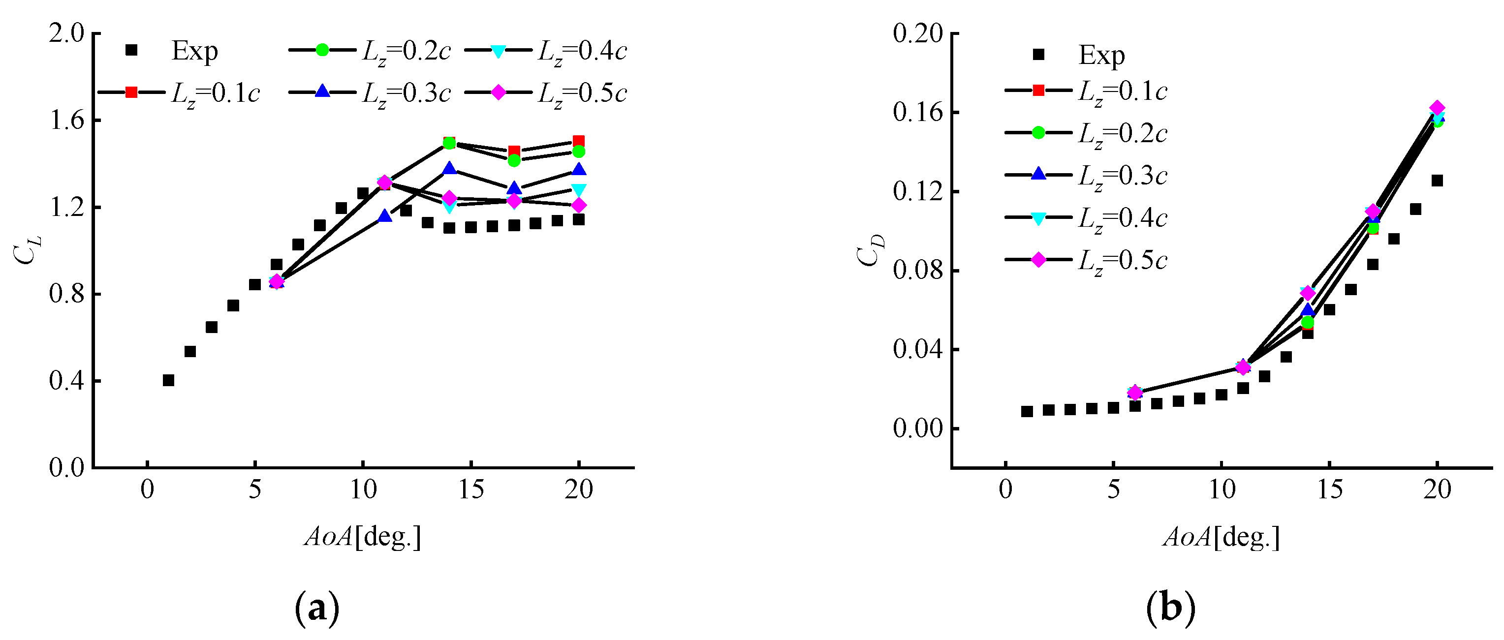
The comparisons of the lift and drag coefficients between the experiments and simulations are shown in Figure 2. The experimental data are depicted by black squares without a solid line. The numerical results are depicted by symbols with solid lines at AOAs of 6°,11°,14°,17° and 20°. The relative errors between the numerical and experimental results are listed in Table 2 and Table 3.
From Figure 2a, it is clear that the discrepancies between the simulations and experiments mainly appear when the AOA is larger than 11°, where all the DDES simulations predict larger lift and drag coefficients. With the increase in the spanwise length, the simulated lift coefficient gradually approaches the experimental value. When the airfoil span length Lz reaches 0.4c and 0.5c, the DDES data agree well with the experiment values. When the AOA is smaller than 11°, the lift coefficient is in the linear region without stall, where all the DDES simulations nearly coincide with each other. Interestingly, the spanwise length has little influence on the aerodynamic performances in the linear region before stall. Even with the shortest span of Lz = 0.1c, the lift and drag coefficients are nearly the same as those of Lz = 0.5c. This gives important information that a narrow span can be used to effectively reduce the total grid number, when simulating the aerodynamic or aeroacoustic performances of airfoils before stall.
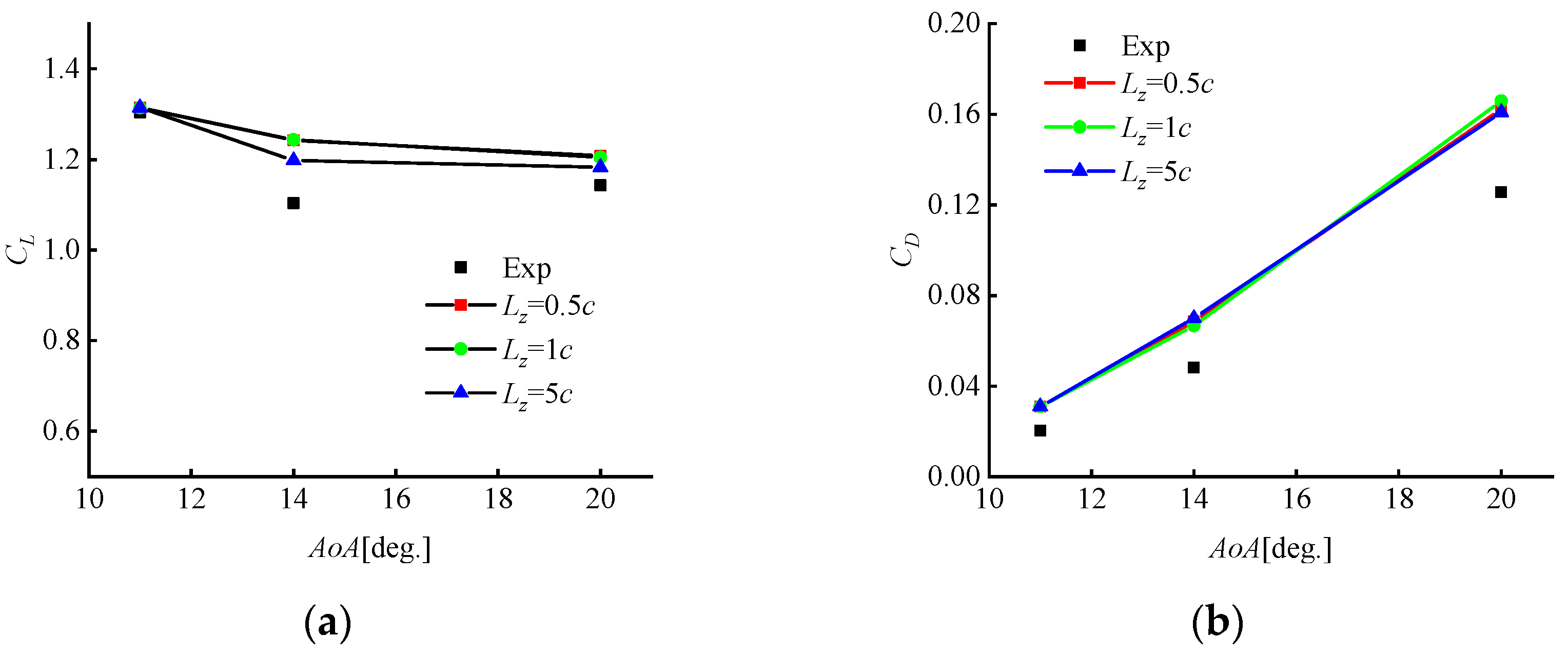
As has been discussed above, the difficulties for simulations mainly appeared with the emergence of stall. Therefore, more simulations were conducted at the AOAs of 11°, 14° and 20°, with the spanwise domain extended to 1 and 5 times the chord length. These simulation results are shown in Figure 3 and their relative errors away from the experimental values are listed in Table 4. It was found that the improvement of accuracy was not obvious when Lz increased from 0.5c to 1c. When the AOA = 14° and 20°, the results of Lz = 5c were the closest to the experiments, with a maximum lift coefficient deviation of less than 10%. This section reveals that different spanwise lengths are needed with reference to the different circumstances in order to improve numerical accuracy over a wide range of AOAs. A larger spanwise domain is needed in the stall and post-stall region because a 3D vortex of larger scale appears. A narrow spanwise length limits the development of the large eddy growth in its spanwise direction, which is demonstrated below.
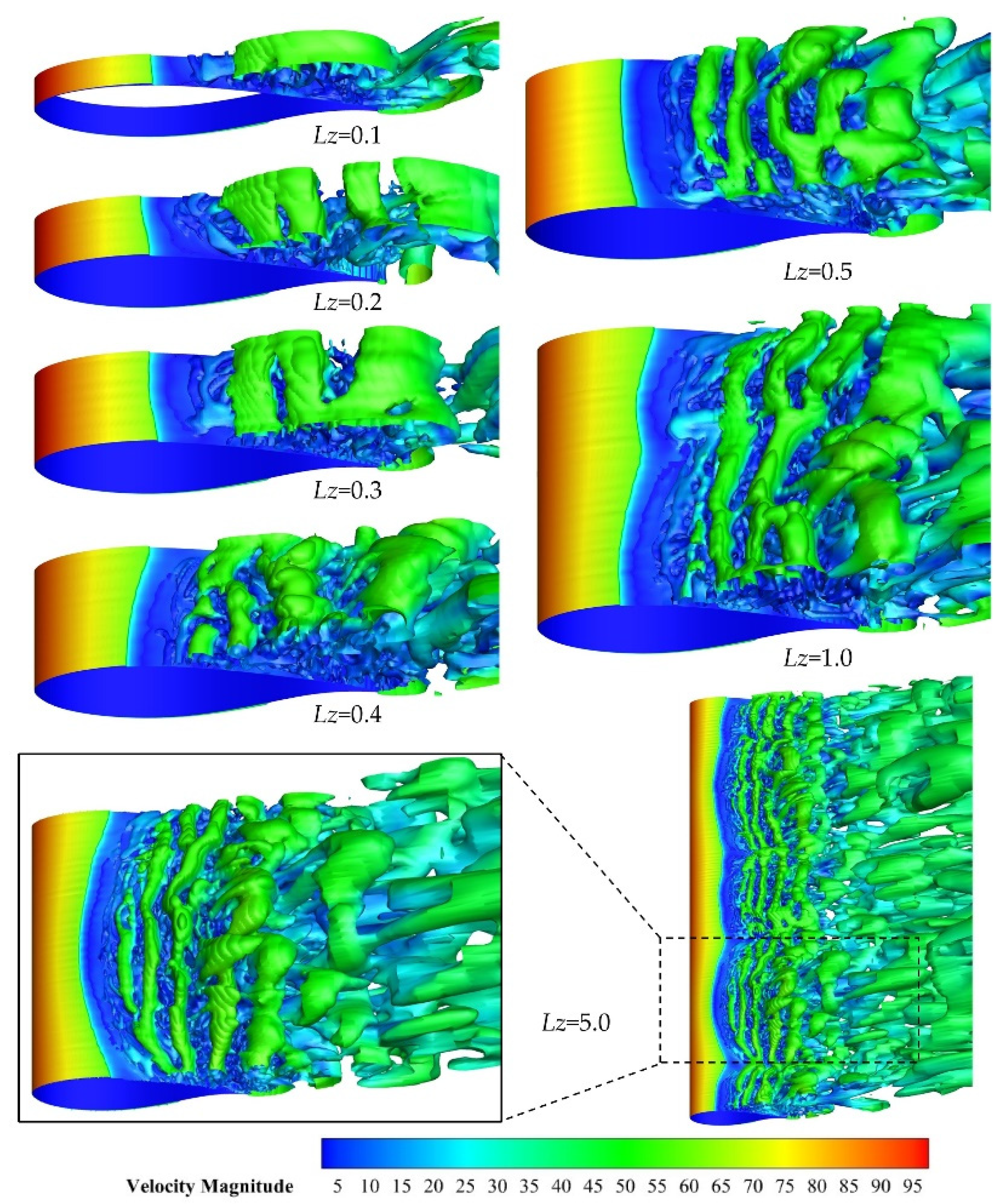
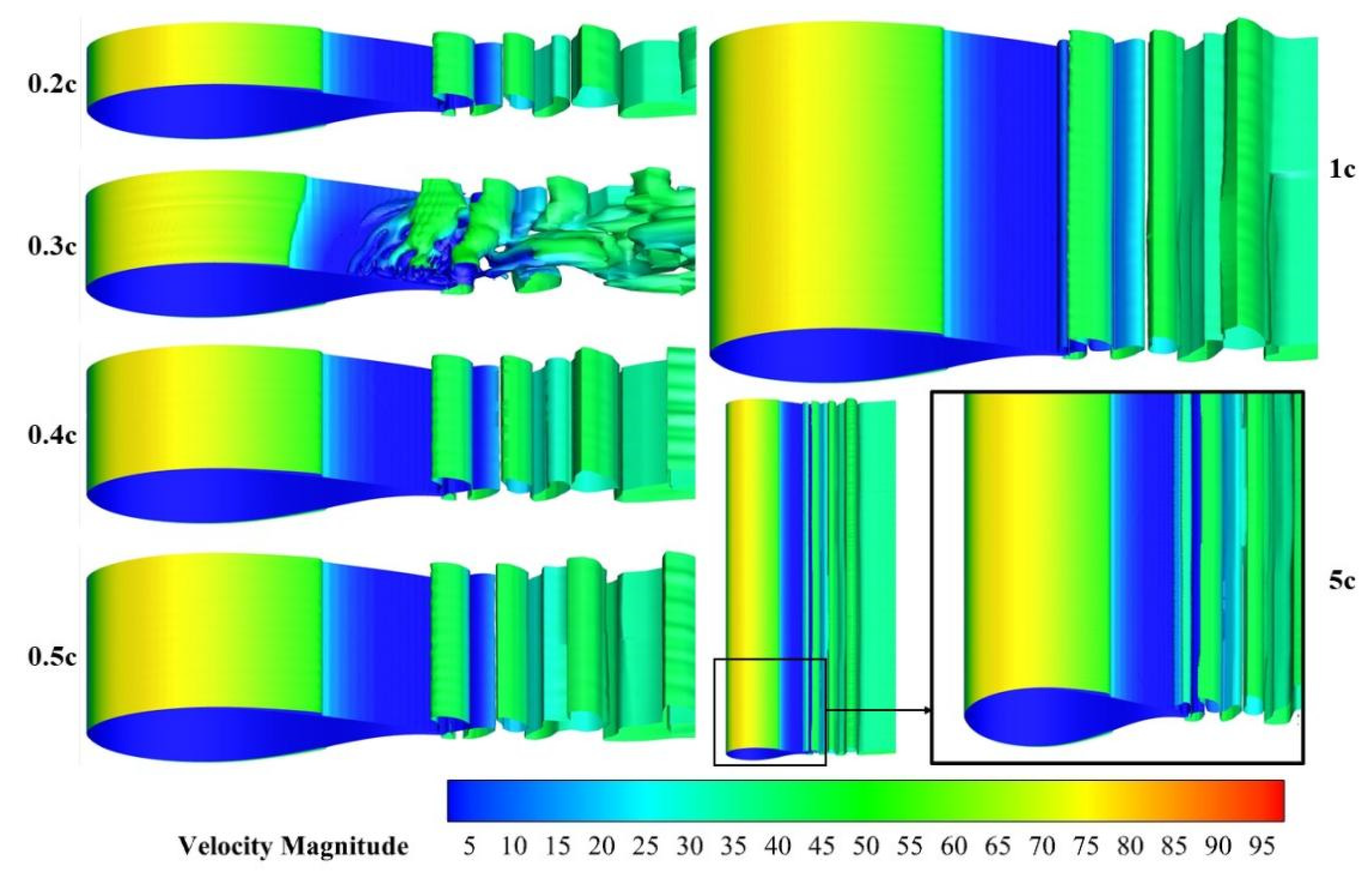
The instantaneous snapshots of the Q-criterion iso-surface, colored by the vorticity magnitude, are shown in Figure 4 for different spanwise domains. The angle of attack AOA = 20° implies deep stall. It is clear that the spanwise length has a significant effect on vortex development. A larger spanwise length leads to a more complex vortex structure and a more pronounced 3D spanwise flow, especially near the trailing edge and in its wake. The most elaborate eddy structures can be found from the case with the largest span of Lz = 5c. What is more, the periodic flow pattern is clearly observed on case Lz = 5c. However, other cases with a shorter span do not show spanwise periodicity. The highest accuracy of case Lz = 5c indicates that the spanwise width should cover at least one spanwise-flow wavelength, to properly simulate the flow under stall. Furthermore, the separation position moves towards the leading edge of the airfoil as the spanwise length increases, which is consistent with the findings shown in Figure 5.
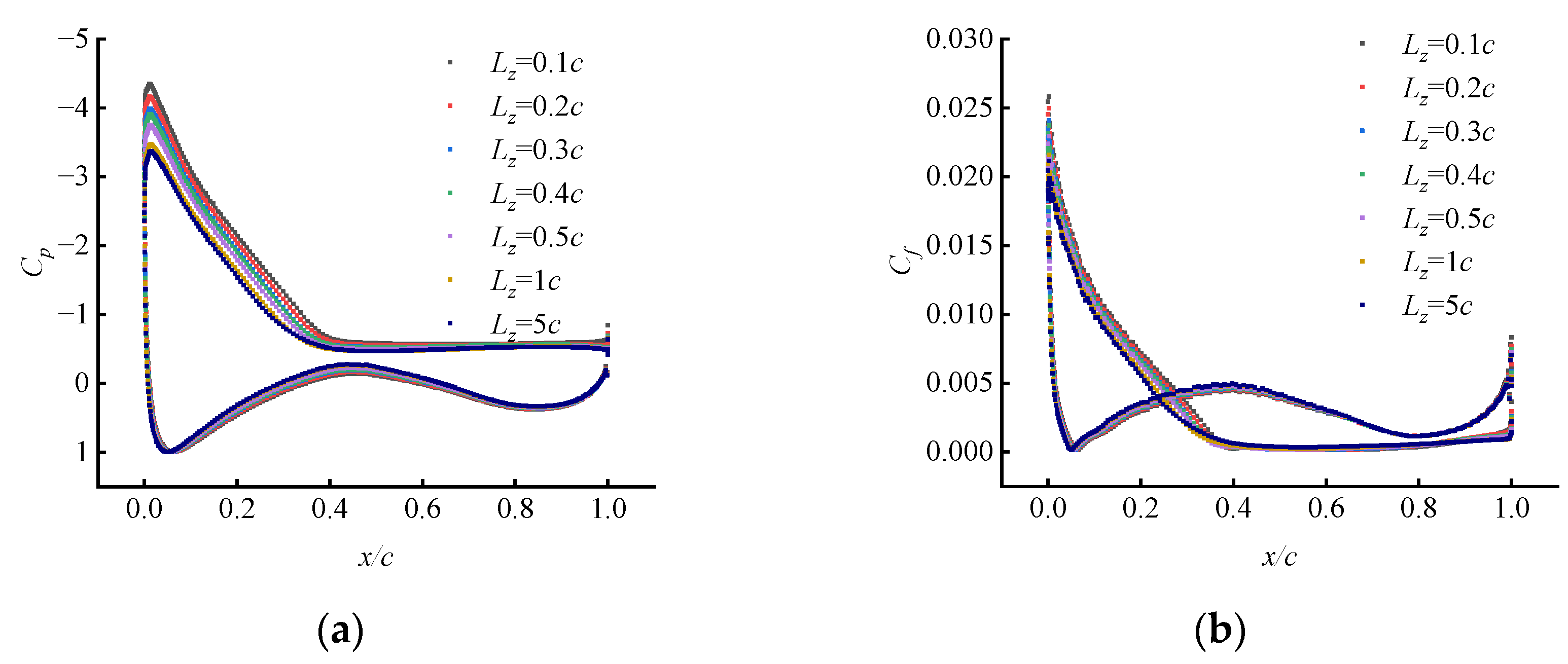
The pressure coefficient Cp and the friction coefficient Cf, which is averaged along a sufficient time period and the whole span, are depicted in Figure 5. Near the chordwise position of x = 0.4c, the Cp curves change the slope, which implies the transition region of separation. As observed, the predicted separation points move a little forward to the leading edge when larger spans are used. Interestingly, the suction peak near the leading edge declines with the decrease in the spanwise length. This explains why the lift coefficient drops when the spans are larger, as is shown in Figure 2 and Figure 3. The separated region in stall affects the attached region.

3.2. The Grid Sensitivity

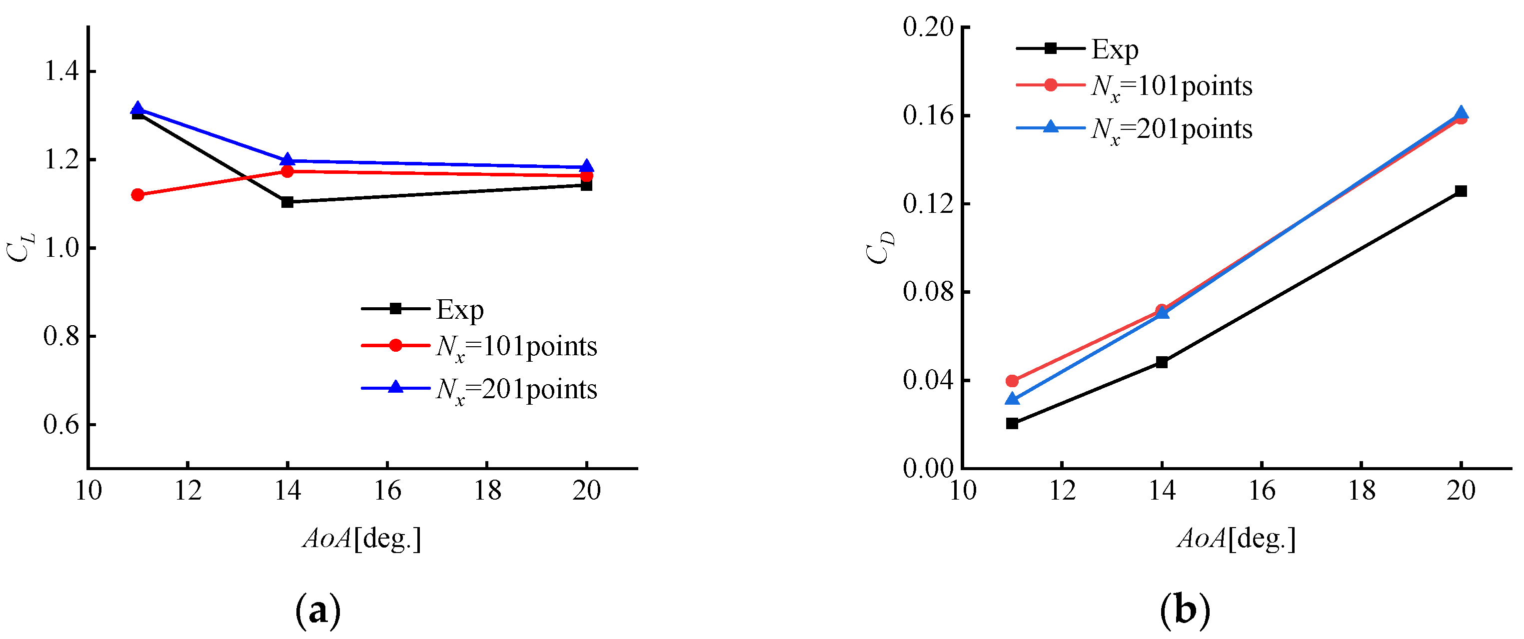
So far, as has been discussed, the case with a spanwise length of 5c is the best configuration. Based on this basic configuration, the sensitivity of the chordwise node density was investigated. Figure 6 shows the lift and drag coefficients from grids with two levels of chordwise node numbers Nx = 101 and 201. The grid with Nx = 101 has chordwise cell scales of about 1/100 of the chord length, and a cell size of 1/200 of the chord length for Nx = 201. As compared with the 201 chordwise node configuration, the case with 101 nodes was not enough to satisfy the required prediction accuracy at the stall angles. The comparisons of the lift and drag coefficients can be found in Figure 6a. At an AOA of 11°, the lift coefficient is much lower than the experimental value. The number or the size of cells are highly case- and methodology-specific. Among the cases studied in this paper, it was found that the number of the chordwise cell size should be smaller than 1/200 of the chord length.
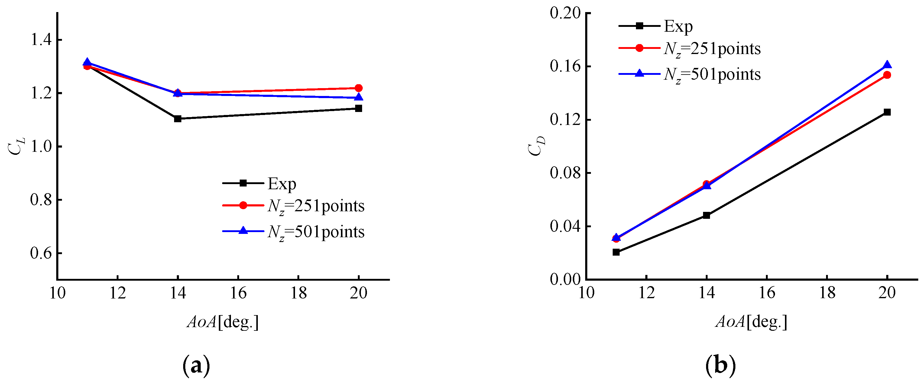
Based on the finest mesh with a spanwise length of 5c, the number of nodes along the same span was deducted from the original 501 to 251 to further investigate the effects of the spanwise node density. Nz = 501 means the spanwise cell scales are 1/100 of the chord length, and 1/50 of the chord length of Nz = 251. The lift and drag coefficients are compared in Figure 7 and Table 5. Surprisingly, very close numerical results were obtained in the stall region. Compared with the results in Figure 2 and Figure 3, the simulation of stall was more sensitive to the spanwise length rather than the spanwise node density.

3.3. The Accurate Prediction of Stall-Starting AOA

It is of vital importance to accurately predict the start of stall. Looking back at Figure 2, it is interesting that the lift coefficient curve of Lz = 0.3c divides the other lines into two groups. The first group, with the spanwise length of less than 0.3c, cannot accurately predict the stall-starting angle. It can be found that the lift coefficients continue to rise after the AOA of 11°. The second group, with the spanwise length of greater than 0.3c, can predict the stall angle perfectly. The lift coefficient curves decline after the AOA of 11°. It can be seen that the appropriate spanwise length plays an important role in the numerical simulation of airfoils at the stall angle.
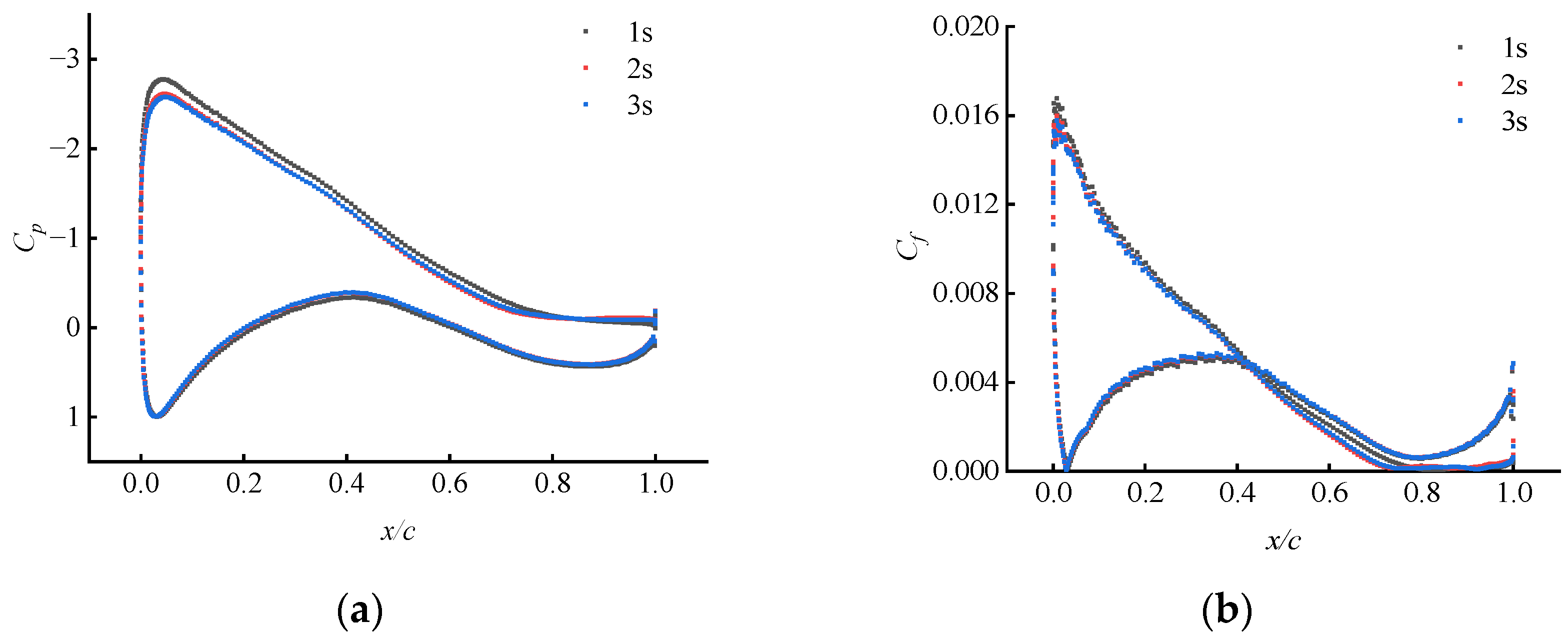
In addition to the spanwise domain and grid density, other factors also affect the numerical simulation. Special attention should be paid to the lift coefficient of Lz = 0.3c. When the AOA equals 11°, the lift coefficient is obviously lower than the other cases, which is shown in Figure 2. It should be noted that the lift and drag coefficients in Figure 2 and in other figures are time-averaged data. If we focus on the transient lift coefficient, it is found that the simulated lift coefficient equals 1.306 at a transient time of 1s, which is close to the experimental value. As the calculation continues, the lift coefficient is reduced to 1.15 at a transient time of 3 s. If we focus on the transient flow field, rather different flow structures can be seen. In Figure 8, the changes in flow-field structures with reference to time are shown. The flow around the airfoil is nearly uniform in the spanwise direction when the calculation time is 1 s. When the time approaches 2 s, the flow field indicates some spanwise fluctuations. In Figure 9, the Cp and Cf distributions are shown for the case with Lz = 0.3c at an AOA of 11°, under different calculation times. Firstly, at the time of 1s, the suction peak near the leading edge is larger than that at a time of 2 s and 3 s. Then, when stepping to 2 s and 3 s, the suction peak drops and the starting position of separation moves towards the leading edge, which makes the averaged lift coefficient drop abnormally to a lower value. Finally, with the time moving on, the suction peak maintains the same level as at 2 s and 3 s, but never recovers to the level at 1 s. This finally leads to an obviously lower averaged lift coefficient, which indicates that there are unknown disturbances affecting the simulation of the flow field between 1 s and 2 s. In Figure 10, all Q-criterion iso-surfaces of different spanwise lengths at an AOA of 11° are shown. The anomalies of Lz = 0.3c due to disturbances are obvious. The reasons for these abnormal changes are worthy of further study.

4. Conclusions

A thick airfoil with a thickness to chord ratio of 30% was simulated utilizing the DDES approach in this paper, and it was analyzed through the lift and drag coefficient, the Q criterion iso-surface, the pressure coefficient and the friction coefficient. Firstly, the influence of spanwise length on the numerical results were studied, with the spanwise length varying from 0.1 to 5 chords. It was found that the spanwise length is of vital importance for the numerical simulation. Under stall, the lift coefficient could not be accurately predicted when the spanwise length was reduced to 0.3 chords. In addition, when the spanwise length was increased to 5 chords, a periodic spanwise flow pattern appeared on the airfoil suction side. Secondly, the grid sensitivity was studied. Among the cases in this study, the chordwise cell scales of 1/100 chord length could not predict the coefficient of lift. However, the spanwise cell size of 1/50 chord length could ensure accurate simulation. The simulation of stall was more sensitive to the spanwise length rather than the spanwise node density. However, it must be remembered that the number or the size of cells are highly case- and methodology-specific. Lastly, it was found that accurate prediction of the stall-starting AOA is highly difficulty. The case with a span length of Lz = 0.3c was a watershed among the cases in this paper. With a spanwise length of 0.3c or smaller, the DDES method failed to predict the stall angle. When the spanwise length was greater than 0.3c, the stall angle could be simulated perfectly. Noticeably, the case with a spanwise length of 0.3c showed abnormal flow-field change at the AOA of 11°, which makes the averaged lift coefficient lower and limits the prediction ability of this configuration. The reasons for these abnormal changes are worthy of further study.

Author Contributions

Conceptualization, Z.S. and R.S.; methodology, W.Z.; software, Z.S. and R.S.; validation, Z.S. and R.S.; formal analysis, W.Z.; investigation, R.S.; resources, W.Z.; data curation, R.S.; writing—original draft preparation, Z.S. and R.S.; writing—review and editing, W.Z. and Z.S.; visualization, J.Y.; supervision, X.L. and W.Z.; project administration, X.L.; funding acquisition, Z.S. All authors have read and agreed to the published version of the manuscript.

Funding

This research was funded by the National Natural Science Foundation of China under grant number 51905469; the National Key Research and Development Program of China under grant number 2019YFE0192600; the Natural Science Foundation of Yangzhou under grant number YZ2019074; and the Natural Science Foundation of Jiangsu Higher Education Institutions of China under grant number 22KJD480003.

Institutional Review Board Statement

Not applicable.

Informed Consent Statement

Not applicable.

Data Availability Statement

Data are available on request due to restrictions, e.g., privacy or ethical restrictions. The data presented in this study are available on request from the corresponding author. The data are not publicly available due to the large volume of CFD data.

Acknowledgments

The authors wish to give thanks to Wen Zhong Shen for his academic comments and support of the parallel computing resources. Thanks should also be given to open funding from the Shanxi Key Laboratory of Industrial Automation, under grant number SLGPT2019KF01-13, for its support on publication.

Conflicts of Interest

The authors declare no conflict of interest.

References

  1. Sun, Z.; Zhu, W.J.; Shen, W.Z.; Zhong, W.; Cao, J.; Tao, Q. Aerodynamic Analysis of Coning Effects on the DTU 10 MW Wind Turbine Rotor. Energies 2020, 13, 5753–5771. [Google Scholar] [CrossRef]
  2. Loth, E.; Steele, A.; Ichter, B.; Selig, M.; Moriarty, P. Segmented Ultralight Pre-Aligned Rotor for Extreme-Scale Wind Turbines. In Proceedings of the 50th AIAA Aerospace Sciences Meeting including the New Horizons Forum and Aerospace Exposition, American Institute of Aeronautics and Astronautics, Nashville, TN, USA, 9 January 2012. [Google Scholar]
  3. Barnes, R.H.; Morozov, E.V. Structural Optimisation of Composite Wind Turbine Blade Structures with Variations of Internal Geometry Configuration. Compos. Struct. 2016, 152, 158–167. [Google Scholar] [CrossRef]
  4. Chen, J.; Wang, Q.; Shen, W.Z.; Pang, X.; Li, S.; Guo, X. Structural Optimization Study of Composite Wind Turbine Blade. Mater. Des. 2013, 46, 247–255. [Google Scholar] [CrossRef]
  5. Sun, Z.; Sessarego, M.; Chen, J.; Shen, W.Z. Design of the OffWindChina 5 MW Wind Turbine Rotor. Energies 2017, 10, 777–796. [Google Scholar] [CrossRef] [Green Version]
  6. Hrgovan, I.; Shen, W.Z.; Zhu, W.J.; Madsen, J.; Hansen, R. Design and Experimental Validation of Thick Airfoils for Large Wind Turbines. In Renewable Energy in the Service of Mankind Vol I: Selected Topics from the World Renewable Energy Congress WREC 2014; Sayigh, A., Ed.; Springer International Publishing: Cham, Switzerland, 2015; pp. 855–863. [Google Scholar]
  7. Zahle, F.; Bak, C.; Sørensen, N.N.; Vronsky, T.; Gaudern, N. Design of the LRP Airfoil Series Using 2D CFD. J. Phys. Conf. Ser. 2014, 524, 12020. [Google Scholar] [CrossRef] [Green Version]
  8. Drela, M. XFOIL: An Analysis and Design System for Low Reynolds Number Airfoils. In Proceedings of the Low Reynolds Number Aerodynamics; Mueller, T.J., Ed.; Springer: Berlin/Heidelberg, Germany, 1989; pp. 1–12. [Google Scholar]
  9. Szydlowski, J.; Costes, M. Simulation of Flow Around a Static and Oscillating in Pitch NACA 0015 Airfoil Using URANS and DES. In Proceedings of the Volume 2, Parts A and B; ASMEDC: Charlotte, NC, USA, 2004; pp. 891–908. [Google Scholar]
  10. Richez, F.; Mary, I.; Gleize, V.; Basdevant, C. Near Stall Simulation of the Flow around an Airfoil Using Zonal RANS/LES Coupling Method. Comput Fluids 2008, 37, 857–866. [Google Scholar] [CrossRef]
  11. Richez, F.; Mary, I.; Gleize, V.; Basdevant, C. Zonal RANS/LES Coupling Simulation of a Transitional and Separated Flow around an Airfoil near Stall. Theor. Comput. Fluid Dyn. 2008, 22, 305–315. [Google Scholar] [CrossRef]
  12. Sandham, N.D. Transitional Separation Bubbles and Unsteady Aspects of Aerofoil Stall. Aeronaut. J. 2008, 112, 395–404. [Google Scholar] [CrossRef] [Green Version]
  13. Almutairi, J.; Jones, L.; Sandham, N. Intermittent Bursting of a Laminar Separation Bubble on an Airfoil. AIAA J. 2010, 48, 414–426. [Google Scholar] [CrossRef]
  14. Fukumoto, H.; Aono, H.; Nonomura, T.; Oyama, A.; Fujii, K. Significance of Computational Spanwise Domain Length on LES for the Flowfield with Large Vortex Structure; American Institute of Aeronautics and Astronautics: Nashville, TN, USA, 4 January 2016; Volume 7. [Google Scholar]
  15. Manni, L.; Nishino, T.; Delafin, P.-L. Numerical Study of Airfoil Stall Cells Using a Very Wide Computational Domain. Comput Fluids 2016, 140, 260–269. [Google Scholar] [CrossRef]
  16. Sharma, A.; Visbal, M. Numerical Investigation of the Effect of Airfoil Thickness on Onset of Dynamic Stall. J. Fluid Mech. 2017, 870, 870–900. [Google Scholar] [CrossRef] [Green Version]
  17. Asada, K.; Kawai, S. Large-Eddy Simulation of Airfoil Flow near Stall Condition at Reynolds Number 2.1 × 10⁶. Phys. Fluids 2018, 30, 85103. [Google Scholar] [CrossRef]
  18. Yalçın, Ö.; Cengiz, K.; Özyörük, Y. High-Order Detached Eddy Simulation of Unsteady Flow around NREL S826 Airfoil. J. Wind Eng. Ind. Aerodyn. 2018, 179, 125–134. [Google Scholar] [CrossRef]
  19. Cui, W.; Xiao, Z.; Yuan, X. Simulations of Transition and Separation Past a Wind-Turbine Airfoil near Stall. Energy 2020, 205, 118003. [Google Scholar] [CrossRef]
  20. Tamaki, Y.; Fukushima, Y.; Kuya, Y.; Kawai, S. Physics and Modeling of Trailing-Edge Stall Phenomena for Wall-Modeled Large-Eddy Simulation. Phys. Rev. Fluid 2020, 5, 74602. [Google Scholar] [CrossRef]
  21. Gleize, V.; Costes, M.; Mary, I. Numerical Simulation of NACA4412 Airfoil in Pre-Stall Conditions. International Journal of Numer. Methods Heat Fluid Flow 2021, 32, 1375–1397. [Google Scholar] [CrossRef]
  22. Menter, F.; Kuntz, M.; Langtry, R. Ten Years of Industrial Experience with the SST Turbulence Model. Turbul. Heat Mass Transf. 2003, 4, 625–632. [Google Scholar]
  23. Menter, F.R. Two-Equation Eddy-Viscosity Turbulence Models for Engineering Applications. AIAA J. 1994, 32, 1598–1605. [Google Scholar] [CrossRef]
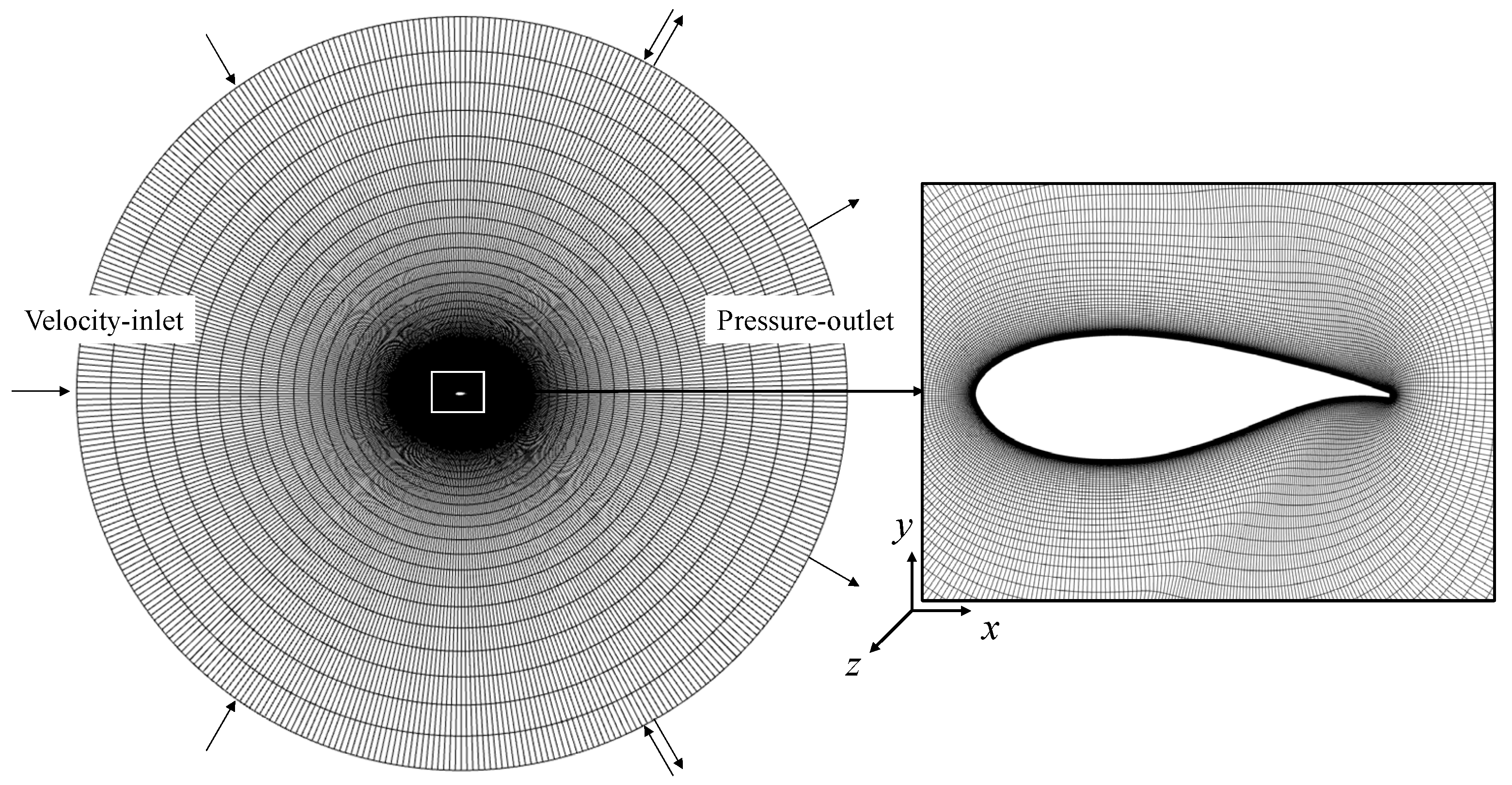
Figure 1. The O-topology mesh and boundary conditions.
Atmosphere 13 01804 g001
Figure 2. Comparisons of experimental and computational lift and drag coefficients: (a) is the CL of simulations and experiments with AOAs of 6°, 11°, 14°, 17° and 20°; (b) is the CD of simulations and experiments with AOAs of 6°, 11°, 14°, 17° and 20°.
Atmosphere 13 01804 g002
Figure 3. Comparison of experimental and computational lift and drag coefficients of Lz = 0.5c, 1c and 5c. (a) is the CL; (b) is the CD.
Atmosphere 13 01804 g003
Figure 4. Iso-surface of Q = 10 by the different spanwise domains at AoA = 20°.
Atmosphere 13 01804 g004
Figure 5. Cp and Cf with different spanwise domains at the angle of attack of 20°: (a) is the Cp; (b) is the Cf.
Atmosphere 13 01804 g005
Figure 6. Experimental and computed lift and drag coefficients with different streamwise node density: (a) is the CL; (b) is the CD.
Atmosphere 13 01804 g006
Figure 7. Experimental and computed lift and drag coefficients with different spanwise node density: (a) is the CL; (b) is the CD.
Atmosphere 13 01804 g007
Figure 8. The Q-criterion iso-surface around the airfoil at an AOA of 11° and at transient times of 1 s (left) and 3 s (right).
Atmosphere 13 01804 g008
Figure 9. Cp and Cf with Lz = 0.3c at an AOA of 11°: (a) is the Cp; (b) is the Cf.
Atmosphere 13 01804 g009
Figure 10. The Q-criterion iso-surface around the airfoil at an AOA of 11° with span lengths from 0.2c to 5c.
Atmosphere 13 01804 g010
Table 1. The summary of settings of different grids.
Lz/cNxNyNzx+y+z+
0.120113411~60011200
0.220113421~60011200
0.320113431~60011200
0.420113441~60011200
0.520113451~60011200
1201134101~60011200
5201134501~60011200
5201134251~60012400
5101134501~120011200
Table 2. The lift coefficient relative error at each AOA under different spanwise lengths.
CL11°14°17°20°
Lz = 0.1c−8.92%0.35%35.69%30.38%31.53%
Lz = 0.2c−8.28%0.75%35.39%26.75%27.47%
Lz = 0.3c−8.97%−11.57%24.45%14.79%19.75%
Lz = 0.4c−8.28%0.75%9.54%9.99%12.51%
Lz = 0.5c−8.28%0.74%12.56%10.19%5.73%
Table 3. The drag coefficient relative error at each AOA under different spanwise lengths.
CD11°14°17°20°
Lz = 0.1c59.54%51.22%9.69%21.70%25.08%
Lz = 0.2c59.91%51.59%11.58%22.40%23.82%
Lz = 0.3c60.04%52.29%23.74%28.24%25.67%
Lz = 0.4c59.91%51.60%43.57%32.02%25.79%
Lz = 0.5c59.91%51.58%42.24%32.29%29.22%
Table 4. The lift and drag coefficient relative errors at each angle of attack under different span lengths.
11°14°20°
Lz = 0.5c0.74%12.56%5.73%
CLLz = 1c0.75%12.64%5.42%
Lz = 5c0.76%8.54%3.50%
Lz = 0.5c51.58%42.24%29.22%
CDLz = 1c51.60%38.47%32.04%
Lz = 5c51.61%45.19%28.07%
Table 5. The lift and drag coefficient errors at each angle of attack under different grid sensitivity.
11°14°20°
Nx = 201, Nz = 501 0.76%8.54%3.50%
CLNx = 101, Nz = 501 −14.12%6.33%1.81%
Nx = 201, Nz = 251 −0.23%8.70%6.68%
Nx = 201, Nz = 501 51.61%45.19%28.07%
CDNx = 101, Nz = 501 93.66%48.84%26.40%
Nx = 201, Nz = 251 49.46%48.34%22.25%
Publisher’s Note: MDPI stays neutral with regard to jurisdictional claims in published maps and institutional affiliations.