Abstract
Traffic information from the distance matrix application program interface (API), which is a part of the Google Maps API service, was used to develop a near real-time traffic emissions inventory in Bangkok. The information provided includes distance and traveling time, which can be used to develop an Underwood traffic model for traffic volume estimation. The speed-dependent emission factors, road distance and traffic volume, which were estimated based on the distance matrix API, and fleet composition, were used to estimate carbon monoxide (CO), hydrocarbon (HC), nitrogen oxide (NOx) and particulate matter (PM) emissions from eight types of vehicles, including passenger cars, motorcycles, pick-ups, taxis, vans, buses, tuk-tuks and trucks. On the weekend, in Bangkok, the traffic released 190 tons/day of CO, 34 tons/day of HC, 55 tons/day of NOx and 3 tons/day of PM. The traffic emissions on a weekday in Bangkok were 209 tons/day of CO, 39 tons/day of HC, 61 tons/day of NOx and 4 tons/day of PM. The spatial and temporal distribution of traffic emissions demonstrate that the area of highest traffic emissions was the center of Bangkok. Therefore, the Google Map API service can be used to develop near real-time traffic emission inventories.
1. Introduction
Bangkok is a megacity and is the economic, financial and tourism center of Thailand. According to INRIX [1], Bangkok was ranked sixteenth out of 1360 cities in the world and first out of 54 cities in Asia in terms of where people spend most time on roads due to traffic congestion. One of the reasons for traffic congestion is the rapid increase in the number of vehicles relative to the speed of road network expansion [2]. There is a high number of old vehicles, particularly vehicles aged more than 10 years [3]. These contribute significantly to the high level of traffic emissions in Bangkok.
Data collected from roadside air quality monitoring stations in Thailand showed that the annual average concentration of fine particulate matter (PM2.5) often exceeded the national ambient air quality standards [4]. Traffic emission is considered as one of the major sources of PM2.5 in Bangkok [5,6]. According to Leong et al. [7] and Wang et al. [8], many factors, such as fuel quality, vehicle operating condition, diurnal traffic patterns and vehicle age affect emissions from in-use vehicles. Around 85% of all NOx emissions from traffic are produced by diesel engines. Moreover, emissions of PM from diesel vehicles are six to ten times higher than those from gasoline vehicles [9,10]. Furthermore, old vehicles produce several unregulated hazardous hydrocarbon (HC)-based air pollutants, such as methane and polycyclic aromatic compounds. These air pollutants can cause several health conditions, including cancer, respiratory-related symptoms and lung disease [11,12].
An emissions inventory is a tool that can be used for managing air quality, along with air quality monitoring and air quality modeling. Emissions inventories are used to identify sources and magnitude of emissions during a specific period in an identified geographical domain. Approaches used for on-road (or traffic) emission’s inventory development can range from top-down (less detail) to bottom-up (more detail) methods depending on the availability of both activity data and information on emission factors. For example, Mohan [13] and Liu et al. [14] estimated traffic emissions in Delhi and urban areas in China, respectively, using detailed activity data, i.e., traveled distance, vehicle type and traffic volume. To obtain this traffic information, significant resources (i.e., time and man-hours) were required for data collection. Conventional data collection methods include counting the number of cars at different intersections and roads at different times and measuring the average speed of vehicles on each road.
Instead of using conventional methods to acquire information on traffic volumes by field survey, traffic flow theory [15] and traffic models [16] can be used to estimate traffic volume based on traffic density and vehicle speed if the width of the road is known [17,18]. With respect to emission factors, the emissions of vehicles traveling at different speeds on the road are not the same [19,20]. For instance, emissions of HC and CO decrease when vehicle speed increases, while emissions of NOx decrease until the optimum speed is achieved before increasing when vehicle speed is increased. Thus, vehicle speed on the road can be used to better select the appropriate vehicle emission factors for vehicles traveling on selected roads.
In this study, the Google map API, called the distance matrix API, which provides details of duration and distance between two points on any road section (starting node and ending node) from the Google map application [21], was used to estimate the average speed on different road sections in Bangkok. This near real-time traffic information from the Google API was used with a traffic model to predict traffic volume and to help in selecting suitable speed-related emission factors to develop a near real-time traffic emission inventory in Bangkok.
2. Methods
The distance matrix API was used to retrieve distance and travel duration data of different road sections in Bangkok which could then be converted to data on average traffic speed. The distance matrix API is a Google service which provides duration and distance data between starting nodes and ending nodes from a Google map application [21]. Users can extract the distance and travel time using programming languages, such as Python. The starting node and ending node can be identified using latitude and longitude co-ordinates on the road. Wagner et al. [22] validated travel time information from the Google API and concluded that it could provide a cost-effective means of developing a traffic-related database. However, accuracy could only be evaluated for large roads, such as freeways, but not for small roads. Thus, the accuracy of data acquired from small roads remained uncertain.
After retrieving distance and travel duration information online, traffic models representing the relationship between traffic volume and traffic speed, including a lane adjustment factor, were developed using traffic information from October 2018 to February 2019, the period before the COVID-19 situation, representing normal traffic patterns in Bangkok. Then, traffic volume data, estimated from the traffic model and lane adjustment factor according to vehicle type and engine technology, were multiplied with speed-related emission factors to produce an estimated near real-time traffic emissions inventory in Bangkok. The near real-time traffic emission inventory for each road segment was developed based on a bottom-up approach, as shown in Equation (1).
where
- = traffic emission of pollutant p on road segment k (g/hr)
- = emission factor for pollutant p from vehicle type i at speed j (g/km)
- = traffic volume of vehicle type i on road segment k (vehicles/hr)
- = length of road segment k (km)
2.1. Traffic Model and Lane Adjustment Factor
The speed of vehicles on the road was calculated from the relationship between distance and traveling time between two points using the distance matrix API. The Python programing language, using the requested parameters provided by Google, was used to automatically retrieve traffic information from the distance matrix API [21]. The coordinates of the starting nodes and the ending nodes were mapped and entered in terms of latitude and longitude co-ordinates in Python using the Google My Maps application to cover all main roads in Bangkok. The term “main road” here refers to public roads that connect the province to districts and sub-districts. The duration and traveling distance were collected every 15 min from the distance matrix API and averaged to produce the 1-hr average speed of vehicles on each road segment. The speeds retrieved every 15 min showed differences in average speeds on the road of up to 2 km/hr within one hour, indicating a good representation of the 1-hr average speed for the road segment. Thus, 15-min intervals were selected to provide information on the 1-hr average speed to save data retrieval costs. The retrieved 1-hr average speed on the road was used as input to the traffic model to estimate the traffic volume for each road segment.
Sirisubtawee [23] applied three traffic models, namely the Greenshield model, Greenberg model and Underwood model, to predict the traffic volume for a three-lane road in Bangkok and found that the Underwood model provided the highest R-squared value between the actual (manually counted) traffic volume and the predicted traffic volume. However, it was noted that the Underwood traffic model was intended for use in free-flow conditions (low density), while other traffic models were better for use with high density traffic [24,25]. In high-density traffic cases, such as Bangkok, other traffic models may perform better than the Underwood traffic model. Thus, potential limitations of the model for the prediction of different traffic conditions require further investigation. In this study, we validated the number of vehicles estimated from the model against the number of vehicles counted manually from CCTV to check whether the Underwood model could be used in Bangkok (Section 3.4). It is, however, recommended that limitations of the model are considered (e.g., traffic conditions, etc.), and validation processes should be applied before the model is used when researching other areas.
The Underwood traffic model (Equation (2)) [16], representing the relationship between the average speed of vehicles on the road (u) and traffic volume (k), was used in this study:
where
u = uf e(−k/km)
- u = speed (km/hr)
- k = density (veh/km)
- uf = free-flow speed (km/hr)
- km = optimum density (veh/km)
To obtain the free-flow speed and optimum density values in Equation (2), the speed of vehicles derived from the distance matrix API was plotted on the Y-axis and the density of vehicles on the road, obtained from video recordings, was plotted on the X-axis. The Underwood model (Equation (2)) was then used to fit the data. The values of the constant for free-flow speed (uf) and the optimum density (km) were obtained from the intercept and slope of the graph. The optimum density is an indicator of the capacity of the road segment (an increase in optimum density results in a higher number of vehicles on the road). Using the estimated free-flow speed (uf) and the optimum density (km), the traffic density (k) estimated from the traffic model was validated against the traffic density derived from manual counting of the number of vehicles on the road for the same hour. Five roads in the center of Bangkok, with one to four lanes, were used in this study.
Next, lane adjustment factors, which were used to adjust the traffic volume based on the number of lanes, were developed. A three-lane road was used as the default number of lanes and the volume of different vehicle types was converted to the volume of passenger car equivalents using the passenger car unit (PCU). Then, the acquired PCU was divided by the traffic volume of the three-lane road to estimate the lane adjustment factor. The relationships between lane adjustment factors and speeds were developed for each number of lanes on the road.
To determine the fleet composition on the road, traffic volume data obtained from video records were manually counted and categorized into eight types of vehicles, including personal cars (PCs), vans, pickups, motorcycles (MCs), tuk-tuks, taxis, buses and trucks. The fleet composition on roads having different numbers of lanes (i.e., 4-lane, 3-lane, 2-lane and 1-lane roads) was observed using traffic video recording to provide data on traffic volume and vehicle composition. The actual traffic volume was used to validate the traffic model and lane adjustment factor using an index of agreement (d) and fractional bias (FB). If the range of d and FB are in the range of agreement (between 0 and 1 for d and between +0.5 and −0.5 for FB), this indicates that the accuracy and performance of the model are acceptable [26,27]. Five roads in the center of Bangkok (Table 1) with 14 closed-circuit television (CCTV) points to monitor traffic were used to collect data on traffic density and fleet composition for 24 h during the study period.

Table 1.
Five roads selected to collect data on traffic density and fleet composition.
2.2. Emission Factors
Emissions from vehicles depend on various factors, such as vehicle type, vehicle age, cumulative mileage and operating condition. Based on various characteristics of in-use vehicles in Bangkok, emission factors were classified according to vehicle type, emission standard and average speed on the road. Eight categories of vehicles were used, as discussed in Section 2.1. Vehicles were assumed to use either gasoline fuel (personal car, taxi, tuk-tuk and motorcycle) or diesel fuel (van, pickup, bus and truck). This assumption was valid for all vehicle types (more than 85% of vehicle registration numbers followed this fuel assumption) except for passenger cars with the fraction of gasoline to total vehicles at around 52% based on vehicle registration data for 2021 in Bangkok. Vehicle emission standards were classified as pre-Euro, Euro I, Euro II, Euro III and Euro IV [28], which are the vehicle emission standards implemented in Thailand.
Emission factors at different vehicle speeds were used to estimate pollutant emissions with the average speed on the road section retrieved from the distance matrix API. To determine the relationship between emission factors for HC, CO, PM and NOx and vehicle speed, data for the emissions of in-use vehicles at different speeds were obtained from the Automotive Emission Laboratory (AEL) of the Thailand Pollution Control Department (PCD) where chassis dynamometers were used to collect emission data from in-use vehicles. Using the chassis dynamometer data, the average speed between 10 and 90 km/hr was linked to the emission of different pollutants. The relationship between emissions and speed was then determined, and equations to estimate emission factors using the average vehicle speed for each vehicle type and the engine standard were derived by curve fitting. Figure 1 shows the PM emission factors vs. vehicle speeds for vans (diesel vehicles).
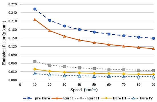
Figure 1.
PM emission factors vs. vehicle speeds for (diesel) vans.
The relationship between the emission factor and the vehicle speed for eight types of vehicles and engine standards is provided in Tables S1–S8 (Supplementary Materials).
2.3. Traffic Emission Inventory
The traffic emission inventory was developed using a bottom-up approach using three major parameters. The first parameter was the traffic volume, which was estimated using the traffic model. The second parameter was the length of the selected road. The third parameter was the emission factor at the average speed of the vehicles on that road link. The overall process for the development of the near real-time traffic emission inventory is presented in Figure 2.
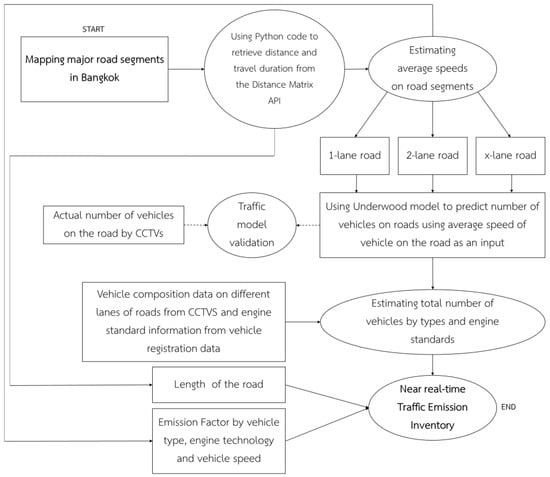
Figure 2.
Overall process for calculating the near real-time traffic emission inventory.
The traffic emissions on 2860 km of the main roads in Bangkok were automatically calculated by retrieving the traffic data from the distance traffic API and the Python code every 15 min. The main roads are the public roads that connect the province with the districts and sub-districts. The total traffic emissions were calculated and extrapolated to a total road length of 5400 km, including both the main and small local roads in Bangkok [29]. The spatial and temporal distribution of emissions were represented by plotting all road links in ArcGIS.
3. Results
3.1. Vehicle Type and Technology in Bangkok’s Fleet
Information on fleet composition in Bangkok was collected by counting vehicle numbers on roads with different lanes using traffic video records. From Figure 3, it can be seen that the proportion of different vehicle types on roads having different numbers of lanes was not the same. However, the pattern was quite similar: PC and MC were found mostly on the roads, followed by taxi and pick-up. There were a larger proportion of large vehicles, i.e., buses and trucks, on roads with more lanes. In contrast, the proportion of motorcycles decreased as the number of lanes increased.
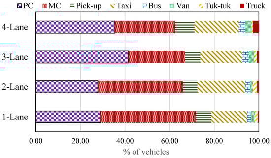
Figure 3.
Proportion of different vehicle types on roads with different number of lanes in Bangkok.
The engine technology of vehicles on the roads was estimated using the enforcement dates of different emission regulations and vehicle registration data from the Department of Land Transport (DLT) in Thailand. It was assumed that vehicles which were registered after the enforcement date for the latest vehicle emission standard in Thailand would follow that emission regulation (Table 2). The proportion of different vehicle types on the road was estimated using data for registered vehicles by age from the DLT (Figure 4). It was assumed that the proportion of different standard vehicles on the road was similar to that from the DLT registration data.
Table 2.
Vehicles ages with different European emission standards in Thailand.
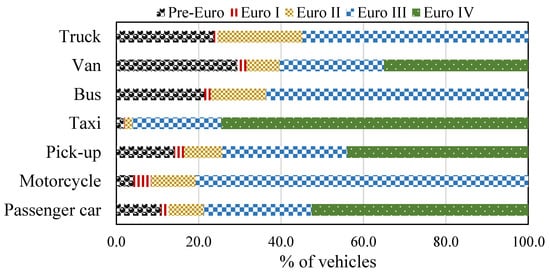
Figure 4.
Proportion of different vehicle technologies for each vehicle type in Bangkok.
3.2. Traffic Models for Bangkok City
Traffic information from the distance matrix API was collected for 24 h in February 2019 and was used to estimate traffic density on the road. The traffic density and speed on the same road were plotted together to determine the relationship between both variables. Traffic models were then developed for roads with a different number of lanes. Figure 5 shows traffic models developed for different numbers of lanes. The traffic model for a three-lane road was selected to represent the main traffic model. It was used with the lane adjustment factor to estimate the traffic volume for different numbers of traffic lanes. Figure 6 shows the speed and density plotted with additional data reflecting a revised relationship between the 1-hr average speed and density. The data used for Figure 6 includes data on speed from different traffic directions on the same road (inbound and outbound) resulting in a slightly weaker relationship (R2) than when using data from one traffic direction alone. Greater fluctuation in average speed was observed at low vehicle density, consistent with the observations of Yu et al. [30]. Therefore, errors in prediction of traffic volume based on the traffic model could increase at high speed when vehicle density is low. The results showed that the average traffic volume was equal to 298 vehicles/hr (based on the actual number of vehicles obtained from CCTV recording during the night) when the average speed on the road was equal to or higher than 46 km/hr.
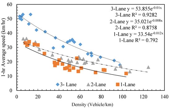
Figure 5.
Traffic models of roads with different number of lanes in Bangkok.
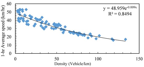
Figure 6.
Traffic models of the 3-lane road with more samples.
3.3. Development of the Lane Adjustment Factor
Chandra et al. [17] developed factors to adjust the number of vehicles using the relationship between capacity and road width. In this study, a similar concept was applied using the number of lanes instead of the road width. The traffic models from Figure 4 were used to develop the lane adjustment factor. The traffic models for the 1-lane, 2-lane and 3-lane roads were used to estimate the traffic volume on the road. The traffic volume for 4-lane roads was then projected based on information on lane, speed and traffic volume. Then, the traffic volume for the 1-lane, 2-lane and 4-lane roads was divided by the traffic volume from the 3-lane road to develop the lane adjustment factors (Figure 7). From Figure 7, it can be seen that the lane adjustment factors for the 1-lane and 2-lane roads decreased when the average speed increased. However, the lane adjustment factor for the 4-lane road increased when the average speed on the road increased. All graphs were fitted with a polynomial equation. If the number of lanes was not three, the lane adjustment factor was used to adjust for the accuracy of the traffic volume using the developed polynomial equations.
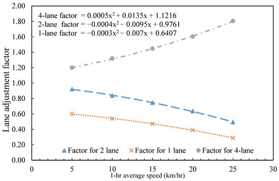
Figure 7.
Adjustment factors for road with different number of lanes.
3.4. Validation of the Traffic Model
The vehicle volume estimated from the traffic model and lane adjustment factor was validated against the actual vehicle volume on the road using an index of agreement and fractional bias. The inputs to the calculation of the index of agreement and fractional bias were the vehicle volume from the Underwood traffic model developed and the actual (manually counted) vehicle numbers on the road derived from CCTV recording. Table 3 shows the results of the model validation using the manually counted traffic volume. For all the roads tested in this study, most of the indices of agreement and fractional biases were within the acceptable range (as discussed in Section 2.1). For the Suthisan Winitchai road (the Sapan-kwai intersection), the fractional bias and the index of agreement were not in the acceptable range. This was because there was a special traffic arrangement to manage traffic congestion on the road during different hours of the day. During rush hour in the evening (from 17.00 hrs to 19.00 hrs), the inbound direction was canceled and changed to an outbound direction to increase the capacity for outbound traffic which involved higher demand in the evening. Although the actual traffic volume for this period should be equal to zero, the distance matrix API still showed the speed on this road. Therefore, time-specific traffic arrangements can create differences between the actual traffic volume and the predicted traffic volume. However, not many roads applied this time-specific arrangement to handle traffic congestion in Bangkok.
Table 3.
The result of the traffic model validation.
3.5. Diurnal Distribution of Traffic Emissions
The diurnal emissions distribution of CO, HC, NOx and PM were estimated for weekdays (from 11 to 13 March 2019) and weekends (on 17 and 31 March 2019) for 24 h. Figure 8 and Figure 9 show the 24-hr traffic emissions on weekdays and weekends, respectively. Emissions during the weekend were lower than those during weekdays, especially at 8.00 hrs. However, the trend in hourly traffic emissions for weekdays and weekends was almost the same. The lowest traffic emissions occurred during the night and increased in the morning. Traffic emissions remained constant in the afternoon and reached a maximum in the evening around 18.00 hrs.
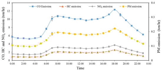
Figure 8.
Diurnal distribution of traffic emissions in Bangkok during weekdays.
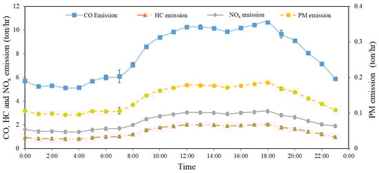
Figure 9.
Diurnal distribution of traffic emissions in Bangkok during weekends.
3.6. Spatial Distribution of Traffic Emissions in Bangkok
Figure 10 shows the spatial distribution of PM emissions for different roads in Bangkok. Other pollutants (CO, HC and NOx) showed similar spatial distribution patterns. Figure 10 was plotted using emissions data estimated for each major road segment in Bangkok; the emissions were overlaid with the corresponding road segment in ArcGIS. Traffic emission on roads in the centre of the city were higher than emissions in border areas. In the centre of the city, there were 110–160 g/hr/km of PM emissions. PM emissions in the border areas ranged from 10–40 g/hr/km. The total traffic emissions were estimated as 8.34 tons/hr, 1.54 tons/hr, 2.42 tons/hr and 0.12 tons/hr for CO, HC, NOx and PM, respectively.
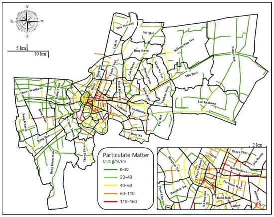
Figure 10.
Spatial distribution of PM on different roads in Bangkok.
To compare traffic emissions observed in this study with other studies, we multiplied emissions found in this study with the ratio of the road length in this study and the road length in the Bangkok Metropolitan Region (BMR), which includes Bangkok and five surrounding provinces, since other studies had previously estimated emissions for the BMR area. Table 4 illustrates that the traffic emissions projected to the BMR area were comparable to the emissions reported in the other three studies. The differences among the emissions estimated from this study and the other three studies were due to differences in the base year, the methodology used (near real-time method vs. conventional method) and emission factors (speed-dependent emission factors vs. average fleet emission factors). For CO, this study estimated CO emissions as 433 kt/yr, while the other studies estimated CO emissions to be in the range 153–371 kt/yr. Since CO emissions are highly related to vehicle speed, CO emissions estimated from speed-dependent emission factors for average speed in the city (and projected to other metropolitan area) may lead to higher emissions estimates than for other studies using fleet average CO emission factors. For HC, NOx and PM, this study estimated emissions to be within the range between the lowest and highest estimations from the other studies. Thus, the near real-time on-road emission estimation method can be used to estimate emissions and produces similar result to those obtained using conventional methods.
Table 4.
Comparison of traffic emission inventories in the BMR area.
3.7. Contribution of Different Vehicle Types to Traffic Emissions in Bangkok
From Figure 11, it can be seen that the number of lanes directly affected vehicle composition on the road and, thus, traffic emissions. The proportion of emissions from small vehicles, such as motorcycles and passenger cars increased as the number of lanes reduced. Moreover, the major sources of CO and HC were from motorcycles, which contributed 64% and 44% of total traffic emissions, respectively. Buses were the major source of NOx and PM, contributing 30% and 45% of total traffic emissions, respectively.
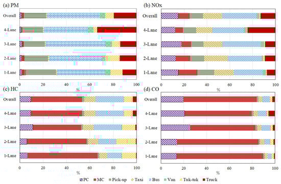
Figure 11.
Contribution of different types of vehicles to total emissions in Bangkok (a) PM; (b) NOx; (c) HC; (d) CO.
4. Conclusions
The Google Maps API was used to develop a near real-time traffic emission inventory in Bangkok. The accuracy of the inventory developed depended on the traffic model, emission factors and traffic information (such as the number of lanes and type of road) employed. The Google Maps API provides traffic information in terms of duration of travel and road length which can be used to estimate the speed of vehicles on the road. The speed of vehicles was used as input to the traffic models to estimate the traffic volume (number of vehicles on the road) and the emission factors (which depend on vehicle speed). The programming language Python was used to access the Google Maps API. The traffic information from the Google Maps API was used to calculate the estimated traffic volume as a basis for automatically developing the emissions inventory for each road. Therefore, the traffic emission for roads in Bangkok could be determined within a short period. Using the Google Maps API and the speed specific emissions factors in this study, the annual traffic emissions in Bangkok in 2019 were estimated to be 87 kt/yr of CO, 16 kt/yr of HC, 25 kt/yr of NOx and 1.4 kt/yr of PM
With respect to the diurnal distribution of traffic emissions, the patterns of traffic emissions on weekdays and weekends were quite similar, except between 5.00hrs and 8.00hrs. However, emissions on weekdays were higher than emissions on weekends. The spatial distribution of traffic emissions on the roads indicated that emissions in the centre of Bangkok were higher than in the border areas due to extreme traffic congestion and a higher number of vehicles on the roads.
In Bangkok, the major contributor to CO and HC emissions was motorcycles, which emitted 64% of CO emissions and 43% of HC emissions. Buses were the largest source of NOx and PM emissions, contributing 30% and 45% of NOx and PM in Bangkok, respectively.
Supplementary Materials
The following supporting information can be downloaded at: https://www.mdpi.com/article/10.3390/atmos13111803/s1, Table S1. Equations for estimating CO emission factor from vehicle speed for light-duty vehicles; Table S2. Equations for estimating CO emission factor from vehicle speed for heavy-duty vehicles; Table S3. Equations for estimating HC emission factor from vehicle speed for light-duty vehicles; Table S4. Equations for estimating HC emission factor from vehicle speed for heavy-duty vehicles; Table S5. Equations for estimating NOx emission factor from vehicle speed for light-duty vehicles; Table S6. Equations for estimating NOx emission factor from vehicle speed for heavy-duty vehicles; Table S7. Equations for estimating PM emission factor from vehicle speed for light-duty vehicles; Table S8. Equations for estimating PM emission factor from vehicle speed for heavy-duty vehicles.
Author Contributions
Conceptualization, E.W.; methodology, S.N., E.W., S.S.; validation, S.N.; formal analysis, S.N. and S.S.; writing—original draft preparation, S.N.; writing—review and editing, E.W. All authors have read and agreed to the published version of the manuscript.
Funding
This research received no external funding.
Institutional Review Board Statement
Not applicable.
Informed Consent Statement
Not applicable.
Data Availability Statement
Not applicable.
Acknowledgments
The authors would like to sincerely thank the Thailand Pollution Control Department for providing emission factors in this study.
Conflicts of Interest
The authors declare no conflict of interest.
References
- INRIX. Bangkok’s Scorecard Report. Available online: http://inrix.com/scorecard-city/?city=Bangkok&index=11 (accessed on 14 July 2022).
- PCD—Pollution Control Department. Report of Situation and Ambient Air Quality in Thailand. Available online: http://air4thai.pcd.go.th/webV2/download.php (accessed on 15 August 2022).
- Caserini, S.; Pastorello, C.; Gaifami, P.; Ntziachristos, L. Impact of the Dropping Activity with Vehicle Age on Air Pollutant Emissions. Atmos. Pollut. Res. 2013, 4, 282–289. [Google Scholar] [CrossRef]
- PCD—Pollution Control Department. Thailand State of Pollution 2020. Available online: https://www.pcd.go.th/wp-content/uploads/2021/03/pcdnew-2021-04-07_06-54-58_342183.pdf (accessed on 14 August 2022).
- Narita, D.; Oanh, N.T.K.; Sato, K.; Huo, M.; Permadi, D.A.; Chi, N.N.H.; Ratanajaratroj, T.; Pawarmart, I. Pollution Characteristics and Policy Actions on Fine Particulate Matter in a Growing Asian Economy: The Case of Bangkok Metropolitan Region. Atmosphere 2019, 10, 227. [Google Scholar] [CrossRef]
- Kanchanasuta, S.; Sooktawee, S.; Patpai, A.; Vatanasomboon, P. Temporal Variations and Potential Source Areas of Fine Particulate Matter in Bangkok, Thailand. Air Soil Water Res. 2020, 13, 1–10. [Google Scholar] [CrossRef]
- Leong, S.T.; Muttamara, S.; Laortanakul, P. Air Pollution and Traffic Measurements in Bangkok Streets. Asian J. Energy Environ. 2002, 3, 185–213. [Google Scholar]
- Wang, X.; Westerdahl, D.; Hu, J.; Wu, Y.; Yin, H.; Pan, X.; Zhang, K. On-road Diesel Vehicle Emission Factors for Nitrogen Oxides and Black Carbon in Two Chinese Cities. Atmos. Environ. 2012, 46, 45–55. [Google Scholar] [CrossRef]
- Reşitoğlu, İ.A.; Altinişik, K.; Keskin, A. The Pollutant Emissions from Diesel-engine Vehicles and Exhaust Aftertreatment Systems. Clean Technol. Environ. Policy 2015, 17, 15–27. [Google Scholar] [CrossRef]
- Singh, A.; Kamal, R.; Ahamed, I.; Wagh, M.; Bihari, V.; Sathin, B.; Kesavanchandran, C.N. PAH Exposure-associated Lung Cancer: An Updated. Meta Anal. 2018, 68, 255–261. [Google Scholar]
- Sahanavin, N.; Prueksasit, T.; Tantrakarnapa, K. Relationship between PM10 and PM2.5 levels in a high-traffic area determined using path analysis and linear regression. J. Environ. Sci. 2018, 69, 105–114. [Google Scholar] [CrossRef] [PubMed]
- WHO—World Health Organization. Global Air Quality Guidelines. Particulate Matter (PM2.5 and PM10), Ozone, Nitrogen Dioxide, Sulfur Dioxide and Carbon Monoxide; World Health Organization: Geneva, Switzerland, 2021; License: CC BY-NC-SA 3.0 IGO.
- Mohan, M.; Bhati, S.; Marappu, P.G. Emission Inventory of Air Pollutants and Trend Analysis Based on Various Regulatory Measures over Megacity Delhi; Air Quality—New Perspective; IntechOpen: London, UK, 2012. [Google Scholar] [CrossRef]
- Liu, Y.-H.; Ma, J.-L.; Li, L.; Lin, X.-F.; Xu, W.-J.; Ding, H. A High Temporal-spatial Vehicle Emission Inventory based on Detailed Hourly Traffic Data in a Medium-sized City of China. Environ. Pollut. 2018, 236, 324–333. [Google Scholar] [CrossRef] [PubMed]
- Immers, L.H.; Logghe, S. Traffic Flow Theory; Katholieke Universiteit Leuven: Heverlee, Belgium, 2002; pp. 1–21. [Google Scholar]
- Qu, X.; Zhang, J.; Wang, S. On the Stochastic Fundamental Diagram for Freeway Traffic: Model Development, Analytical Properties, Validation, and Extensive Applications. Transp. Res. Part B: Methodol. 2018, 104, 256–271. [Google Scholar] [CrossRef]
- Chandra, S.; Upendra, K. Effect of Lane Width on Capacity under Mixed Traffic Conditions in India. J. Transp. Eng. 2003, 129, 155–160. [Google Scholar] [CrossRef]
- Moses, R.; Mtoi, E.; McBean, H.; Ruegg, S. Development of Speed Models for Improving Travel Forecasting and Highway Performance Evaluation; Department of Transportation: Tallahassee, FL, USA, 2013.
- Pelkmans, L.; Debal, P. Comparison of On-road Emissions with Emissions Measured on Chassis Dynamometer Test Cycles. Transp. Res. Part D Transp. Environ. 2006, 11, 233–241. [Google Scholar] [CrossRef]
- Jing, B.; Wu, L.; Mao, H.; Gong, S.; He, J.; Zou, C.; Song, G.; Li, X.; Wu, Z. Development of a Vehicle Emission Inventory with High Temporal–spatial Resolution based on NRT Traffic Data and Its Impact on Air Pollution in Beijing—Part 1: Development and Evaluation of Vehicle Emission Inventory. Atmos. Chem. Phys. 2016, 16, 3161–3170. [Google Scholar] [CrossRef]
- Google-Developers. Developer Guide Distance Matrix API. Available online: https://developers.google.com/maps/documentation/distance-matrix/intro (accessed on 25 August 2019).
- Wagner, J.M.S.; Eschbach, M.; Vosseberg, K.; Gennat, M. Travel Time Estimation by means of Google API data. IFAC PapersOnLine 2020, 15434–15439. [Google Scholar] [CrossRef]
- Sirisubtawee, S. Development of Temporal Distribution of Traffic Emission Using Google Traffic Application Program Interface. Available online: http://203.159.12.58/ait-thesis/detail.php?id=B02703 (accessed on 7 October 2022).
- Edie, L.C. Car-Following and Steady-State Theory for Noncongested Traffic. Oper. Res. 1961, 9, 66–76. [Google Scholar] [CrossRef]
- Heydecker, B.G.; Addison, J.D. Analysis and Modeling of Traffic Flow Under Variable Speed Limits. Transp. Res. Part C Emerg. Technol. 2011, 19, 206–217. [Google Scholar] [CrossRef]
- Willmott, C.J.; Robeson, S.M.; Matsuura, K. A Refined Index of Model Performance. Int. J. Climatol. 2012, 32, 2088–2094. [Google Scholar] [CrossRef]
- Demirarslan, K.O.; Doğruparmak, Ş.Ç. Determining Performance and Application of Steady-state Models and Lagrangian Puff Model for Environmental Assessment of CO and NOx Emissions. Pol. J. Environ. Stud. 2016, 25, 83–96. [Google Scholar] [CrossRef]
- PCD—Pollution Control Department. Vehicle Emission Standard and Management Report; PCD: Bangkok, Thailand, 2012.
- BMA-CPS. Report of Road Network and Special Road in Bangkok. Available online: http://cpd.bangkok.go.th:90/web2/strategy/reportstudy50/Infrastruc (accessed on 15 May 2020).
- Yu, C.; Zhang, J.; Yao, D.; Zhang, R.; Jin, H. Speed-density Model of Interrupted Traffic Flow based on Coil Data. Mob. Inf. Syst. 2016. [Google Scholar] [CrossRef]
- IIASA—International Institute for Applied Systems Analysis. GAINS Online. Available online: https://gains.iiasa.ac.at/models/ (accessed on 14 July 2022).
- Cheewaphongphan, P.; Junpen, A.; Garivait, S.; Chatani, S. Emission Inventory of On-Road Transport in Bangkok Metropolitan Region (BMR) Development during 2007 to 2015 Using the GAINS Model. Atmosphere 2017, 8, 167. [Google Scholar] [CrossRef]
- Kim Oanh, N.T. A Study in Urban Air Pollution Improvement in Asia; Asian Institute of Technology: Bangkok, Thailand, 2017. [Google Scholar]
Publisher’s Note: MDPI stays neutral with regard to jurisdictional claims in published maps and institutional affiliations. |
© 2022 by the authors. Licensee MDPI, Basel, Switzerland. This article is an open access article distributed under the terms and conditions of the Creative Commons Attribution (CC BY) license (https://creativecommons.org/licenses/by/4.0/).