Article

Cyclonic and Anticyclonic Asymmetry of Reef and Atoll Wakes in the Xisha Archipelago

South China Institute of Environmental Sciences, Ministry of Ecology and Environment, Guangzhou 510655, China
*
Authors to whom correspondence should be addressed.
Atmosphere 2022, 13(10), 1740; https://doi.org/10.3390/atmos13101740
Submission received: 30 September 2022 / Revised: 15 October 2022 / Accepted: 18 October 2022 / Published: 21 October 2022
(This article belongs to the Special Issue Air-Sea Interaction: Modeling and Dynamics)

Abstract

:
A high-resolution (∼500 m) numerical model was used to study the reef and atoll wakes in the Xisha Archipelago (XA) during 2009. Statistical analyses of simulation data indicated strong cyclonic dominance in the mixing layer (above ∼35 m) and weak anticyclonic dominance in the subsurface layer (35∼160 m) for both eddies and filaments in the XA. The intrinsic dynamical properties of the flow, such as the vertical stratification and velocity magnitude, and the terrain of reefs and atolls had a significant effect on the asymmetry. Without considering the existence of reefs and atolls, the “background cyclonic dominance” generated under local planetary rotation ( f 4.1 × 10 5 s−1) and vertical stratification (with mean Brunt–Väisälä frequency N = 0.02 s−1 at 75 m) was stronger for filaments than eddies in the upper layer from 0∼200 m, and the larger vorticity amplitude in the cyclonic filaments could greatly enhance the cyclonic wake eddies. Furthermore, inertial–centrifugal instability induced selective destabilization of anticyclonic wake eddies in different water layers. As the Rossby number (Ro) and core vorticity (Burger number, Bu) decreased (increased) with the water depth, a more stable state was achieved for the anticyclonic wake eddies in the deeper layer. The stratification and slipping reefs and atolls also led to vertical decoupled shedding, which intensified the asymmetry.

1. Introduction

Oceanic wake eddies and turbulence usually occur in areas of islands, atolls, and reefs under the comprehensive influence of density stratification and planetary rotation [1,2,3,4,5]. This regime is mainly characterized by the island Rossby number (Ro), Burger number (Bu), Reynolds number (Re), and Ekman number (Ek), e.g., [6]. A strict symmetry between cyclones and anticyclones is found in the quasigeostrophic limit (Ro ≪ 1) [7]. However, this symmetry is usually broken by a finite Ro number [8,9]. Either cyclonic or anticyclonic eddies may become predominant in the oceanic wake [10,11,12,13]. For the mesoscale eddy wake ( r m a x R d with r m a x denoting the characteristic radius of an eddy and R d as the first baroclinic radius), when the Bu and island Ro numbers are both small, the flow will follow the frontal geostrophic regime [14], leading to the more coherent and stable anticyclones than the cyclones [12]. For some extreme cases, only the anticyclonic vortex street can be found behind the island, and coherent cyclones will not appear at all [15]. For the submesoscale eddy wake ( r m a x < R d ), both the Bu and island Ro numbers increase, and the relationship between Ro and the local amplitude of the vorticity ζ / f is not well established. In other words, the dissipation (related to Re) is important to balance the relationship. Thus, inertial–centrifugal instability (ICI) may induce selective instability in the anticyclonic vorticity regions [13]. Studies have shown that the strong stratification coupled with moderate dissipation can strongly stabilize intense submesoscale anticyclones [16,17].
The Xisha Archipelago (XA), located in the tropical region, is composed of several coral reefs, including Bei Reef, Huaguang Reef (HR), Panshi Yu, Yuzhuo Reef (YR), and Lanhua Reef, three larger atolls called Yongle Atoll (YA), Xuande Atoll (XDA), and Xuande East Atoll (XEA), and several small islands, such as Yongxing Island and Zhongjian Island [18] (see Figure 1). The XA is close to the northwest of the South China Sea (SCS). Due to the seasonally reversing monsoons, a basin-scale cyclonic circulation in winter and an anticyclonic circulation in summer an be found in the SCS [19,20,21]. Many cyclones and anticyclones are embedded in the basin-scale circulation, forming a multi-eddy structure [22]. Many surveys have shown that the mesoscale eddies are active in the upper waters in the XA area [23,24,25]. The SCS Western Boundary Current (WBC) is a major component of the SCS circulation [25,26,27], and it changes significantly on seasonal and interannual time scales [25]. In summer, the energetic WBC east of Vietnam passes through the north of the SCS, and anticyclonic circulations are often generated [22,28], whereas it flows southward in winter [25,29], which greatly affects the XA area. In general, a strong northeastward (southwestward) current with the maximum velocity of 1 m/s (exceeding 1 m/s) can be observed near the XA area in the summer (winter) [24,25,29,30]. The ocean dynamics of the XA area are linked to the presence of the Tropical Oceanic Monsoon Climate Zone [31]. In the XA, the sea surface temperature (SST) exhibits obvious seasonal [32] and intraseasonal [33] variations, with a rapid increase and decrease in the SST during the spring and autumn, respectively. These variations are strongly related to the sea surface wind, which affects the net surface heat flux (exactly the latent heat flux) and then controls the seasonal and intraseasonal variations in the SST [32,33]. Thus, the shift of the monsoons induces a half-year cycle in the latent heat flux, as well as the SST.
Submesoscale wake eddies have been observed on the downstream sides of atolls and reefs in the XA [13,34]. Cyclonic dominance has been observed at the surface, which is attributed to the ICI [34]. In the activated upper layer (0∼200 m) of the XA, the intrinsic dynamics such as those of the current and stratification may be very different according to the depth, and they vary with the seasons. Thus, the eddy shedding process and cyclone–anticyclone asymmetry may also be different. A similar phenomenon was studied by Roullet and Klein [11], who performed an ideal numerical simulation of geophysical turbulence characterized by a finite Ro number (∼0.6). This simulation included the active upper boundary and interior dynamics, which is similar to a real marine environment, such as in the XA area. Their results indicated strong cyclonic dominance in the upper layers, which was stronger for filaments than vortices. Furthermore, under strong stratification, vertical decoupled eddy shedding appeared downstream of the slipping seamounts [35].
Most of the studies mentioned above were based on laboratory experiments and ideal numerical simulations. However, in actual marine environments, the real topography such as the XA reefs and atolls developed from carbonate platforms [36], variable vertical stratification [37,38], and currents [24] may greatly change the process, thereby leading to complicated physical dynamics, as well as cyclone and anticyclone asymmetry in the island wakes. To the best of our knowledge, the variations in the cyclonic and anticyclonic asymmetry of reef and atoll wakes in the XA are not well known, especially in the vertical direction. In this study, we investigated the vortical asymmetry of reef and atoll wakes in the XA. High-resolution numerical simulations were first conducted by employing the unstructured grid finite-volume community ocean model (FVCOM) [39,40,41]. Cyclonic and anticyclonic asymmetry in the wakes was then examined, and the physical process was studied.

2. Model and Data

2.1. XA-FVCOM

The XA-FVCOM is a high-resolution regional model designed to simulate the sub-mesoscale wake eddies in the XA [13]. The horizontal resolution ranges from ∼500 m around the reefs (atolls) to ∼8.8 km at the open boundary, in order to conform to the Global HYCOM grid. A uniform σ -coordinate was used in the vertical, with a total of 80 layers. The vertical grid resolution was maintained at ∼10 m in the XA. The XA-FVCOM was driven by 3-hourly Global HYCOM/NCODA oceanic reanalysis data [42,43] and 6-hourly NCEP CFSR atmospheric reanalysis data (wind stress, long wave–short wave irradiance, and evaporation–precipitation at the surface of the sea). The temperature and salinity fields of the XA-FVCOM were initialized by the Global HYCOM. The model was spun up from undisturbed sea surface elevation and zero velocity. More details of the XA-FVCOM can be found in our previous study [13].
The simulation was integrated for 14 months (covering the period from 1 November 2008 to 31 December 2009). The external time step was 2.5 s, and the internal time step was 5 s. The established solution was achieved after the second month (spin-up period). Thus, only the results obtained after 1 January 2009 were analyzed.

2.2. Observational Data

The simulated results were compared with several observations including in situ data, Argo data, and satellite data.
The in situ data from two stations (Points A and B in Figure 2d) in the XA were first collected: Point A stands for a tidal gauge station monitoring sea surface elevation from June 2007 to December 2013, with a 10 min sampling frequency; Point B stands for a subsurface buoy, which is loaded with one downward 150 kHz acoustic Doppler current profiler (ADCP) and one upward 75 kHz ADCP in order to cover the whole water column. The in situ data were provided by the Lake-Watershed Science Data Center, National Earth System Science Data Sharing Infrastructure, National Science & Technology Infrastructure of China (http://lake.geodata.cn (accessed on 7 October 2017)).
Hydrographic data obtained from Argo floats (ID 2901144 and ID 2901145) were also used to compare the ocean with the temperature and salinity vertical profiles produced by the numerical simulations. The Argos were present in the XA from 9 August to 27 December 2009.
The advanced very-high-resolution radiometer (AVHRR) SST data with a resolution of 1.1 km were obtained from the CoastWatch program [44]. The error was within ± 0.5 °C. The sea surface height and geostrophic current data obtained from the weekly AVISO (http://www.aviso.oceanobs.com (accessed on 7 October 2017)) were also used to validate the model.

2.3. Model Validation

The surface circulation of the model result was first validated by the in situ and AVISO data. The modeled daily surface elevation was compared with the in situ and weekly AVISO data, as shown in Figure 2a, which indicates that the overall trend was simulated well during 2009. Compared with the in situ data, the root-mean-squared error of the modeled surface elevation was small (∼0.069 m). The changes in the XA regional mean current are presented in Figure 2b. Compared with the weekly AVISO data, the model satisfactorily represented the annual variation in the current (at a depth of 15 m). It should be noted that the AVISO data only contained geographic components. Our modeling results could represent abundant instant current events. The modeling results and observed data indicated that the current strengthened from March to July and from September to November, and it remained weak from December to February in 2009. As shown in Figure 2c, the general trend of the vertical distribution of the daily mean horizontal velocity magnitudes in the upper seawater was also captured by the XA-FVCOM. Figure 2d compares the annual averaged AVISO observations and FVCOM results in 2009. The modeling results accurately represented the mean surface elevation and geostrophic current in the region. The presence of cyclonic and anticyclonic mesoscale eddies was observed in the west and east of the XA, respectively. Thus, the annual mean current in the XA was northeastward.
The model results also indicated that the XA-FVCOM was in good agreement with the thermodynamic properties found in the XA. Indeed, the model accurately reproduced the SST cycle and vertical temperature profiles during 2009. Figure 3a shows the good agreement of the SST between the model outputs and AVHRR data, where the root-mean-squared error was ∼0.69 °C. The observations and model showed that the SST increased from 29 January to 9 July, before decreasing from 9 July to 29 January, with large fluctuations from late August to early September in 2009. The warmest season occurred from June to September. By contrast, the coldest season occurred between December and February, and the minimum values occurred in 29 January. The XA was characterized by a northwest/southeast SST gradient, as shown by the AVHRR remote sensing data and modeling results (Figure 3b). Vertical profiles based on the means and standard deviations of the temperature and salinity are plotted in Figure 3c (right) for the different sites represented by red dots in Figure 3c (left). The Argos were present in the XA area from 9 August to 27 December in 2009. The vertical profiles of the modeled temperature and salinity were in good agreement with the observations. According to the modeled results, the upper thermocline was located between 18 and 148 m [45]. The simulation performance assessment results indicated that the model could reproduce the main surface circulation and thermodynamics in the oceanic region of the XA.

3. Cyclone–Anticyclone Asymmetry in the XA

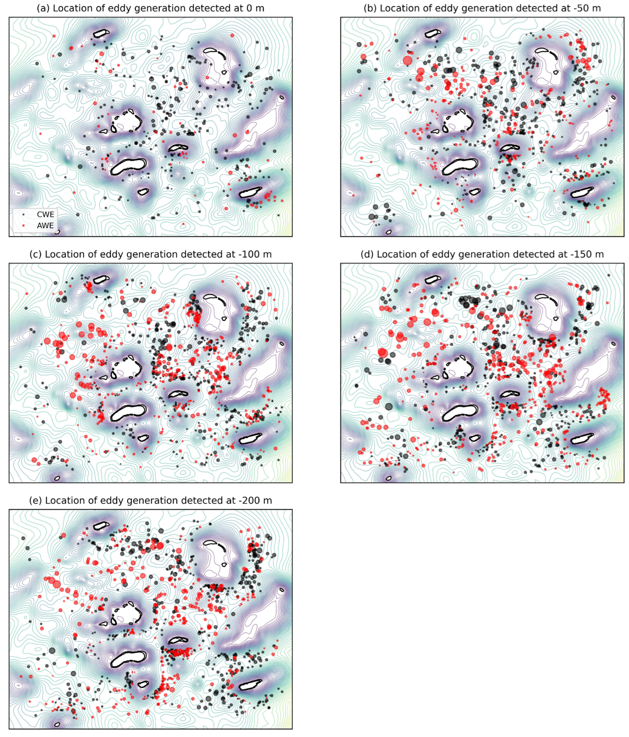
3.1. Wake Eddy Shedding Process

In the XA, the wakes of the reefs and atolls change with the seasons due to the active WBC and mesoscale eddies. In order to provide insights into the cyclone–anticyclone asymmetry of the wake eddies, the instant evolution of the wake eddies between 0 and 200 m based on the sequential maps of vorticity is shown in Figure 4. The boundaries of the coherent wake eddies detected by the vector-geometry-based eddy detection algorithm (VGED) [46] are also depicted. We used the VGED to automatically identify the characteristics of the eddies such as the eddy core, sign, boundary, radius, and trace. Each eddy core was detected based on a point with a minimum velocity and the surrounding velocity vector rotating around it. Eddy boundaries are defined as the outermost closed streamline around the core, across which velocity magnitudes are still increasing in the radial direction. The eddy radius is calculated as the mean distance between the eddy core and all the points defining the boundaries. Once eddies have been detected at each time step, the eddy trace can be tracked using the method proposed by [46]. The XA-FVCOM data were first interpolated into the structured mesh grid with a resolution of 0.005 ° × 0.005 ° to meet the requirements of the VGED. The vorticity maps were characterized by the distribution of eddies coupled with many filaments, especially in the surface layer. In the upper 50 m, the cyclonic wake eddies (CWEs) were clearly merging filaments and small eddies. By contrast, in the layer from 150∼200 m, the anticyclonic wake eddies (AWEs) were activated.
Interestingly, the wake eddies became decoupled in the vertical direction (see Figure 4 at different depths), i.e., rather than each eddy shedding in a vertically uniform manner, each reef (atoll) elevation shed eddies independently and almost as a two-dimensional plane. The eddy scale and shedding frequency varied with depth. For example, the eddy distribution at 0 m was completely different from that at 200 m. Similar results were obtained in a previous study [35] by using a three-dimensional computational model of an idealized sloping seamount in a rotating, stratified flow. Their results showed that the vertical coherence of the wake eddies was strongly dependent on the buoyancy frequency N and Coriolis parameter f, and the decoupled shedding regime was characterized by strong density stratification and weak planetary rotation, as discussed in Section 4.

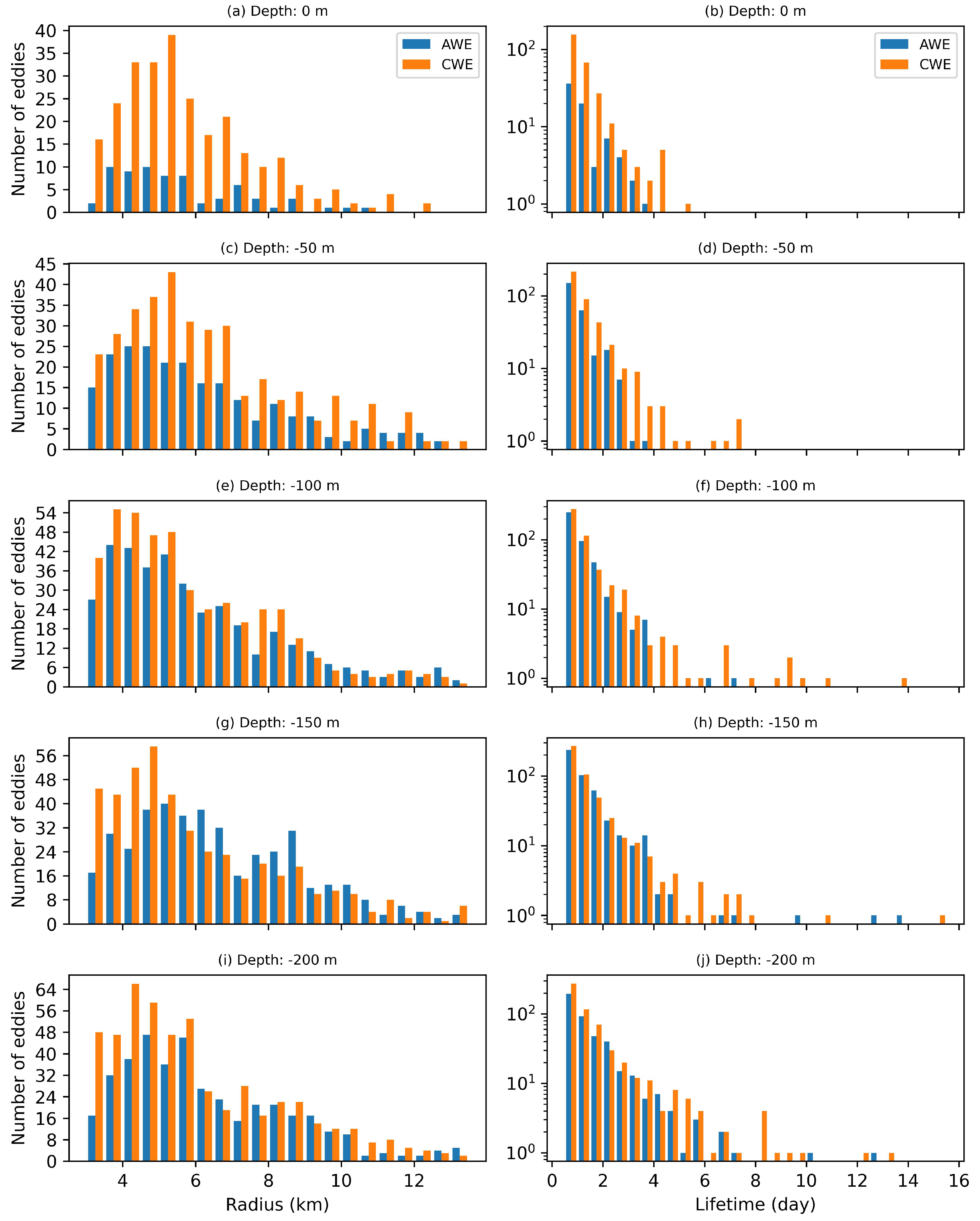
3.2. Cyclone–Anticyclone Asymmetry

Different features of the CWEs and AWEs were found in the decoupled shedding regime. In the surface layer (0∼50 m), the CWEs were generally coherent, and they were always detected by the VGED; however the AWEs could hardly be detected. Thus, the lifetimes of AWEs were short, and they were strongly disturbed and became incoherent after their generation. However, at the subsurface (∼150 m), the wake eddies with a longer lifetime detected by the VGED were both CWEs and AWEs. In general, the current and vorticity decreased with the depth. Due to the vertical distribution of the currents and sloping reefs (atolls) (see Figure 1) in the XA area, the AWEs detected at the subsurface were generally larger and weaker than the CWEs at the surface. According to our previous studies [13], AWEs are more unstable than CWEs due to the ICI, and a moderate incoming velocity and eddy radius are needed to maintain the stability of AWEs.
The statistical results for all the wake eddies formed in 2009 also showed the difference between cyclones and anticyclones. The total number of CWEs and AWEs in the water layer above 200 m generated throughout 2009 is shown in Table 1, and their initial locations are indicated in Figure 5. The number of CWEs increased from 278 at 0 m to 570 at 200 m. By contrast, the number of AWEs increased from 73 at 0 m to 471 at 150 m and then decreased to 431 at 200 m. Due to the ICI, the number of AWEs was clearly less than that of CWEs in the water layer above 50 m. These results also suggest that the AWEs were more stable at 150 m, where the maximum number of AWEs occurred. The initial positions of the eddies were basically around the atolls and reefs, such as YA, HR, YR, XDA, and XEA. Furthermore, the CWEs and AWEs that appeared in different water layers were mainly distributed on the eastern and western sides of the atolls and reefs, respectively (see Figure 5), which indicates that many eddies were formed by the northward incoming flow. Research on the maximum size of the detected wake eddies in their lifetimes showed that, due to the limitations of resolution, their distributions were similar to a mixture of Gaussians without an inferior tail (see Figure 6). By contrast, the distribution of the lifetimes decreased exponentially within 0.5∼16 days, and most of the eddies had lifetimes shorter than 4 days. According to Figure 6, the cyclonic dominance was quite obvious for most of the eddy scales in the water layer above 50 m. However, in the water layer from 100∼200 m, the CWEs and AWEs were mostly symmetric.
The asymmetry was also examined using the probability density function (PDF) of ζ / f as a function of depth (Figure 7a). As shown in Figure 7a, the skewness of ζ / f , represented by the black curve, indicated vortical asymmetry near the upper boundary and the dominance of cyclonic structures in the first 35 m. The skewness became negative between 35 and 160 m in the water layer where the kinetic energy was smaller. The relative vorticity structures involved both coherent eddies and filaments with small-scale elongated structures (see Figure 4). The classical Okubo–Weiss (OW) criterion, defined as C O W =( σ 2 ζ 2 ) / f 2 with σ = ( u x 2 v y 2 ) 2 + ( v x 2 + u y 2 ) 2 , was used to partition the eddies from filaments. We defined eddies as structures with C O W < 0.05 at the upper boundary and filaments as structures with C O W > 0.05 . Figure 7b,c show the PDFs of ζ / f for filaments and eddies. The filaments and eddies had asymmetric PDFs indicating cyclonic dominance in the first 90 m and 40 m, respectively. The anticyclonic dominance was between 90 and 150 m for filaments and between 40 and 160 m for eddies. The skewness of the filaments was obviously greater than that for eddies. These results clearly confirmed that, near the upper boundary, the asymmetry of filaments was stronger than that of eddies.

4. Discussion

Our numerical results indicated strong cyclonic dominance in the surface layer (above ∼35 m) and weak anticyclonic dominance in the subsurface layer (35∼160 m) for both eddies and filaments in the XA. The intrinsic dynamical properties of the flow [6,13] and terrain, such as reefs (atolls), may have significantly affected the asymmetry [35].

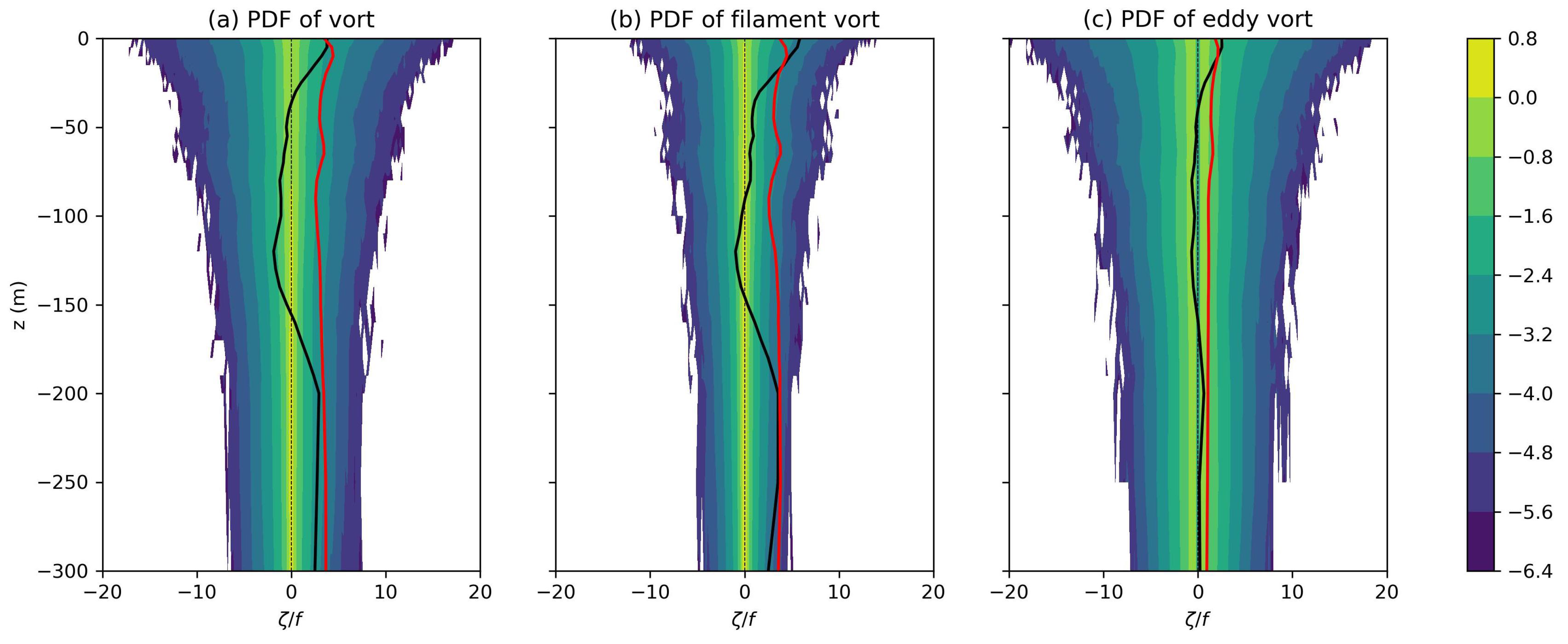
4.1. Intrinsic Dynamical Properties of the Flow

In order to study the complex phenomenon, an additional simulation was also performed without reefs and atolls (flat bottom) in the XA. The PDFs of ζ / f clearly showed that cyclonic dominance was stronger for filaments than eddies in the upper layer from 0∼200 m, which is in accordance with a previous study by Roullet and Klein [11], where their geophysical turbulent simulations with an active upper boundary (strong stratification in the upper 1500 m) and interior dynamics (weak stratification below 1500 m) indicated strong cyclonic dominance in the first 600 m, where the stratification was strongest. In the XA, the larger vorticity amplitude in cyclonic filaments in the surface could have greatly enhanced the CWEs (see Figure 4 for an example) to some extent, thereby leading to cyclonic dominance. We refer to the cyclonic dominance without reefs (atolls) as the “background cyclonic dominance”.
To provide deeper insights into this phenomenon, the vertical stratification of the XA represented by the Brunt–Väisälä frequency N = g ρ 0 ρ z is depicted in Figure 8a. This figure shows that the extreme value of N was located about 75 m below the sea surface in the winter (December to February) and about 50 m below in the summer (June to August). The extreme annual mean value of N = 0.02 s−1 was located at 75 m. The Brunt–Väisälä frequency was much larger in the summer than the winter, thereby suggesting strong stratification in the summer. The simulated annual mean mixing layer depth (MLD) was found from 5∼63 m (see Appendix A), with smaller values downstream of the reefs and atolls [47]. In the XA areas, the MLD values were generally smaller than 35 m. Interestingly, it appeared that the cyclonic dominance was stronger in the mixed layer (see Figure 7), where the stratification was not as significant.
Indeed, according to Lazar et al. [16], under stratification and rotation, the ICI may have a selective effect on viscous eddies and lead to cyclone–anticyclone asymmetry. Three dimensionless parameters were considered comprising the Rossby number Ro = V m a x f r m a x , Burger number Bu = R d r m a x 2 , and Ekman number Ek = κ z f h c 2 , where V m a x , r m a x are the maximum velocity and corresponding radius of the eddy, κ z is the vertical diffusivity, and h c is the thickness of the surface current. The following equation is used to judge the linearly unstable anticyclonic Rankine eddies:
1 Ek 8 | a 0 | 3 3 Bu Ro 2 | 2 Ro + 1 | 7 = f ( Ro , Bu ) ,
where the first zero of the Airy function | a 0 | = 2.3381 . Ro has a significant effect on the stability of an anticyclonic eddy. Stratification is quantified at the submesoscale by Bu. A larger Bu (strong stratification) can help stabilize AWEs. The statistical results for the parameters related to the AWEs detected from 0 to 200 m are shown in Table 2. Clearly, decreasing trends were found in Ro and the core vorticity | ζ 0 / f | , and the lifetimes tended to increase with the water depth, thereby demonstrating that the AWEs achieved a more stable state in the deeper layer. Interestingly, the Bu value in the layer below 50 m was almost twice that in the layer above 50 m, thereby indicating weak stratification in the upper 50 m.
It is well known that, when a weak oceanic current encounters a large island, both the wake eddies and wake flow will satisfy the geostrophic equilibrium with the corresponding Ro 1 . However, when an oceanic current encounters a small island with a characteristic length smaller than the local R d , then both Ro and Bu increase. The relationship between Ro and ζ / f is not well established, and it crucially depends on the dissipation. Thus, the ICI may induce the selective destabilization of anticyclonic eddies in regions. These results indicate that the stability of AWEs is affected mainly by the ICI, but the extent of this effect varies with the depth. In particular, strong vertical stratification enhances the stability of AWEs to some extent.

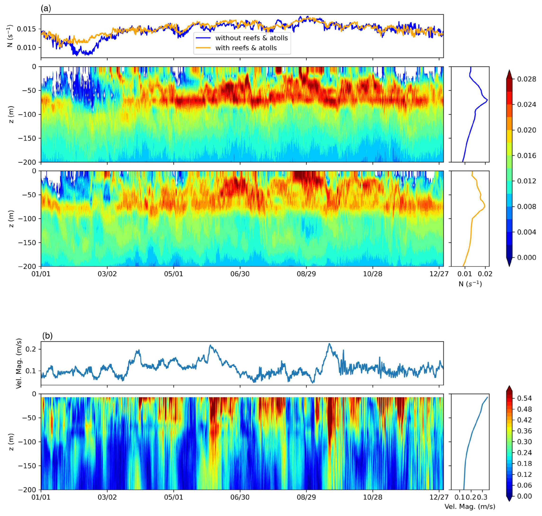
4.2. Effects of Reefs and Atolls

Compared with the simulations without reefs and atolls, we also found that, due to the lack of reefs (atolls), the weak anticyclonic dominance in the subsurface layer depicted in Figure 7 was rarely observed. We checked the time sequences for the skewness of the vorticity PDFs with and without reefs (atolls) and found that the background cyclonic dominance was present at 0∼200 m for most of the time when the reefs (atolls) did not appear (Figure 9). Thus, wake eddies and turbulence occurred when the reefs (atolls) were present, and the ICI induced selective destabilization of AWEs in different water layers. When superimposing the background cyclonic dominance, it indicated strong cyclonic dominance in the surface layer and weak anticyclonic dominance in the subsurface layer in the XA.
The presence of reefs and atolls not only leads to the appearance of turbulent wakes, but also greatly intensifies the vertical mixing. As a result, the vertical stratification was greatly weakened and the value of N was reduced (see Figure 8a). The sloping reefs (atolls) (see Figure 1) coupled with stratification also led to vertically decoupled shedding, which intensified the cyclone–anticyclone asymmetry. According to Perfect et al. [35], this decoupling exists in weak rotation (high Ro) and strong stratification. Thus, the Burger number written in another form as Bu = ( Ro Fr ) 2 was used to predict vertically decoupled eddies. In the XA, the mean Bu numbers of AWEs detected by the VGED were between 52.5 and 95.1 in different upper water layers. In general, the AWEs of the XA belonged to submesoscale eddies, and they had large Bu numbers, which are associated with barotropic flow (stronger stratification impedes the perturbation of isopycnals). Figure 4 shows the strong vertically decoupled shedding process coupled with a strong northeastward incoming flow during April 13 and 17 in our simulation. This type of incoming flow is very common in the XA area (see Figure 2b and Figure 8b), which suggests that vertical decoupling is also very common.
The above analyses clearly show a significant impact on the local ocean dynamics, especially the cyclone–anticyclone asymmetry, due to the presence of reefs and atolls in the XA. Interestingly, the latest research of Qin et al. [36] demonstrated that oceanographic currents have a control on the carbonate growth. As the XA is a reef–beach system developed on the isolated carbonate platforms, their study showed that differences in hydrodynamic energy related to currents and waves driven by East Asian monsoon winds were responsible for asymmetrical backstepping at the Xuande platform margins in the latest Miocene to the Early Pliocene [36]. According to our study, the cyclone–anticyclone asymmetry in different seasons deeply changed the local hydrodynamic environment (such as the uplift and downwelling of the isopycnal caused by CWEs and AWEs, respectively [13]). It may further control the carbonate growth in the XA. There seems to be some interaction between the formation of coral reefs (atolls) and the incoming currents, as well as their current wakes. In some extreme cases, the nutrient-rich waters caused by the upwelling can kill off isolated platforms on continental margins [48,49]. All these studies demonstrate the far-reaching effect of local hydrodynamics on the formation of reef and atoll topography, to a certain extent. Among them, the cyclone–anticyclone asymmetry may help interpret the asymmetry of carbonate growth. However, a carefully study is needed.

5. Conclusions

In this study, we demonstrated the cyclone–anticyclone asymmetry of the reef and atoll wakes in the XA using the high-resolution XA-FVCOM, which was validated by in situ, AVISO, AVHRR, and Argo data. Strong cyclonic dominance in the surface layer (above ∼35 m) and weak anticyclonic dominance in the subsurface layer (35∼160 m) for both eddies and filaments were observed in the XA. In the rotation and stratification processes, without considering the existence of reefs and atolls, the background cyclonic dominance was stronger for filaments than eddies in the upper layer from 0∼200 m. In addition, the larger vorticity amplitude in the cyclonic filaments greatly enhanced the CWEs. Furthermore, the ICI induced selective destabilization of the AWEs in different water layers. Considering the stratification and special reef and atoll topography in the XA, vertical decoupled shedding could also have intensified the asymmetry. All of these effects led to the strong cyclonic dominance in the surface layer and weak anticyclonic dominance in the subsurface layer. However, further studies such as in situ observations are needed to confirm these phenomena. Some interesting topics such as the interaction between the formation of coral reefs (atolls) and the current wakes, the different effects of AWEs and CWEs on nutrient or pollutant transport, and the biological effects of the reef (atoll) wakes are worth studying in the future.

Author Contributions

Formal analysis, Y.Y.; Investigation, S.Q. and S.L.; Project Administration, Z.Z.; Resources, J.Y.; Validation, Z.C.; Writing—Original Draft, Z.Z. All authors have read and agreed to the published version of the manuscript.

Funding

This research was funded by projects supported by the Ministry of Industry and Information Technology of the People’s Republic of China (Project No. [2019]357), the National Natural Science Foundation of China (Project No. 41506202), the Natural Science Foundation of Guangdong (Project No. 2018A030313316), and the Science and Technology Projects in Guangzhou (Project No. 202102020917).

Data Availability Statement

HYCOM/NCODA Global reanalysis data at https://www.hycom.org (accessed on 14 May 2022); sea surface height and geostrophic current data at http://www.aviso.oceanobs.com (accessed on 12 April 2021); South China Sea and Adjacent Seas Data Center, National Earth System Science Data Sharing Infrastructure, National Science & Technology Infrastructure of China, at http://ocean.geodata.cn (accessed on 7 October 2017).

Conflicts of Interest

The authors have no conflicts of interest to declare.

Abbreviations

The following abbreviations are used in this manuscript:
XAXisha Archipelago
SCSSouth China Sea
WBCWestern Boundary Current
CWEscyclonic wake eddies
AWEsanticyclonic wake eddies
VGEDvector-geometry-based eddy detection algorithm
ICIinertial–centrifugal instability
OWOkubo–Weiss
PDFprobability density function
MLDmixing layer depth

Appendix A

In the SCS, the following criterion is widely used to compute the MLD [37,50]:
MLD = z ( T 10 + Δ T ) ,
where ΔT = −0.8 °C and T 10 is the temperature at a depth of 10 m.

References

  1. Doty, M.; Oguri, M. The island mass effect. ICES J. Mar. Sci. 1956, 22, 33–37. [Google Scholar] [CrossRef]
  2. Arístegui, J.; Tett, P.; Hernández-Guerra, A.; Basterretxea, G.; Montero, M.; Wild, K.; Sangrá, P.; Hernández-Leon, S.; Canton, M.; García-Braun, J.; et al. The influence of island-generated eddies on chlorophyll distribution: A study of mesoscale variation around Gran Canaria. Deep Sea Res. Part I: Oceanogr. Res. Pap. 1997, 44, 71–96. [Google Scholar] [CrossRef]
  3. Caldeira, R.; Groom, S.; Miller, P.; Pilgrim, D.; Nezlin, N. Sea-surface signatures of the island mass effect phenomena around Madeira Island, Northeast Atlantic. Remote Sens. Environ. 2002, 80, 336–360. [Google Scholar] [CrossRef]
  4. Caldeira, R.; Marchesiello, P.; Nezlin, N.; DiGiacomo, P.; McWilliams, J. Island wakes in the Southern California Bight. J. Geophys. Res. Ocean. 2005, 110, 1–12. [Google Scholar] [CrossRef]
  5. Andrade, I.; Sangrà, P.; Hormazabal, S.; Correa-Ramirez, M. Island mass effect in the Juan Fernández Archipelago (33 °S), Southeastern Pacific. Deep Sea Res. Part I: Oceanogr. Res. Pap. 2014, 84, 86–99. [Google Scholar] [CrossRef]
  6. Stegner, A. Oceanic island wake flow in laboratory. Modelling Atmospheric and Oceanic Flows Insights from Laboratory Experiments and Numerical Simulations, 1st ed.; John Wiley & Sons: Hoboken, NJ, USA, 2014. [Google Scholar]
  7. McWilliams, J.C.; Weiss, J.B.; Yavneh, I. Anisotropy and coherent vortex structures in planetary turbulence. Science 1994, 264, 410–413. [Google Scholar] [CrossRef] [Green Version]
  8. Yavneh, I.; Shchepetkin, A.F.; Mcwilliams, J.C.; Graves, L.P. Multigrid solution of rotating, stably stratified flows. J. Comput. Phys. 1997, 136, 245–262. [Google Scholar] [CrossRef]
  9. Koszalka, I.; Bracco, A.; Mcwilliams, J.C.; Provenzale, A. Dynamics of wind-forced coherent anticyclones in the open ocean. J. Geophys. Res. Ocean. 2009, 114, C08011. [Google Scholar] [CrossRef] [Green Version]
  10. Raapoto, H.; Martinez, E.; Petrenko, A.; Doglioli, A.M.; Maes, C. Modeling the wake of the Marquesas Archipelago. J. Geophys. Res. Ocean. 2018, 123, 1213–1228. [Google Scholar] [CrossRef] [Green Version]
  11. Roullet, G.; Klein, P. Cyclone-anticyclone asymmetry in geophysical turbulence. Phys. Rev. Lett. 2010, 104, 218501. [Google Scholar] [CrossRef]
  12. Calil, P.H.; Richards, K.J.; Jia, Y.; Bidigare, R.R. Eddy activity in the lee of the Hawaiian Islands. Deep-Sea Res. Part II Top. Stud. Oceanogr. 2008, 55, 1179–1194. [Google Scholar] [CrossRef]
  13. Zhao, Z.; Li, J.; Zhao, W.; Yang, J.; Qi, S.; Xu, M. A numerical study of island wakes in the Xisha Archipelago associated with mesoscale eddies in the spring. Ocean Model. 2019, 139, 101406. [Google Scholar] [CrossRef]
  14. Cushman-Roisin, B. Frontal geostrophic dynamics. J. Phys. Oceanogr. 1986, 16, 132–143. [Google Scholar] [CrossRef]
  15. Perret, G.; Stegner, A.; Farge, M.; Pichon, T. Cyclone-anticyclone asymmetry of large-scale wakes in the laboratory. Phys. Fluids 2006, 18, 036603. [Google Scholar] [CrossRef] [Green Version]
  16. Lazar, A.; Stegner, A.; Heifetz, E. Inertial instability of intense and stratified anticyclones. Part I: Linear analysis and marginal stability criterion. J. Fluid Mech. 2013, 732, 457–484. [Google Scholar] [CrossRef] [Green Version]
  17. Lazar, A.; Stegner, A.; Caldeira, R.; Dong, C.; Didelle, H.; Vuiboud, S. Inertial instability of intense and stratified anticyclones. Part II: Laboratory experiments. J. Fluid Mech. 2013, 732, 485–509. [Google Scholar] [CrossRef]
  18. Ye, Z.; He, Q.; Zhang, M.; Han, C.; Li, H.; Ju, L.; Wu, J. Classification and characteristics of islands in the Xisha Archipelago. Mar. Geol. Quat. Geol. 1985, 5, 1–13. [Google Scholar]
  19. Dale, W. Wind and drift currents in the South China Sea. Malays. J. Trop. Geogr. 1956, 8, 1–31. [Google Scholar]
  20. Metzger, E. Upper ocean sensitivity to wind forcing in the South China Sea. J. Oceanogr. 2003, 59, 783–798. [Google Scholar] [CrossRef]
  21. Wang, G.; Su, J.; Chu, P. Mesoscale eddies in the South China Sea observed with altimeter data. Geophys. Res. Lett. 2003, 30, 2121. [Google Scholar] [CrossRef] [Green Version]
  22. Nan, F.; He, Z.; Zhou, H.; Wang, D. Three long-lived anticyclonic eddies in the northern South China Sea. J. Geophys. Res. Ocean. 2011, 116, 1–15. [Google Scholar] [CrossRef]
  23. Hou, H.; Xie, Q.; Xue, H.; Shu, Y.; Nan, F.; Yin, Y.; Yu, F. Formation of an anticyclonic eddy and the mechanism involved: A case study using cruise data from the northern South China Sea. J. Oceanol. Limnol. 2019, 37, 1481–1494. [Google Scholar] [CrossRef]
  24. Shu, Y.; Xue, H.; Wang, D.; Xie, Q.; Chen, J.; Li, J.; Chen, R.; He, Y.; Li, D. Observed evidence of the anomalous South China Sea western boundary current during the summers of 2010 and 2011. J. Geophys. Res. Ocean. 2016, 121, 1145–1159. [Google Scholar] [CrossRef]
  25. Wang, D.; Liu, Q.; Xie, Q.; He, Z.; Zhuang, W.; Shu, Y.; Xiao, X.; Hong, B.; Wu, X.; Sui, D. Progress of regional oceanography study associated with western boundary current in the South China Sea. Chin. Sci. Bull. 2013, 58, 1205–1215. [Google Scholar] [CrossRef] [Green Version]
  26. Li, L. Seasonal circulation in the South China Sea-a TOPEX/POSEIDON altimetry study. Acta Oceanol. Sin. 2000, 22, 13–26. [Google Scholar]
  27. Wang, G.; Wang, C.; Huang, R.X. Interdecadal variability of the eastward current in the South China Sea associated with the summer Asian monsoon. J. Clim. 2010, 23, 6115–6123. [Google Scholar] [CrossRef] [Green Version]
  28. Hwang, C.; Chen, S. Circulations and eddies over the South China Sea derived from TOPEX/POSEIDON altimetry. J. Geophys. Res. Ocean. 2000, 105, 23943–23965. [Google Scholar] [CrossRef]
  29. Hu, J.; Kawamura, H.; Hong, H.; Qi, Y. A review on the currents in the South China Sea: Seasonal circulation, South China Sea warm current and Kuroshio intrusion. J. Oceanogr. 2000, 56, 607–624. [Google Scholar] [CrossRef]
  30. Chi, P.C.; Chen, Y.; Lu, S. Wind-driven South China Sea deep basin warm-core/cool-core eddies. J. Oceanogr. 1998, 54, 347–360. [Google Scholar] [CrossRef]
  31. Chen, X. The basis of modern climatology. In The Basis of Modern Climatology; Nanjing University Press: Nanjing, China, 2014; pp. 53–56. [Google Scholar]
  32. Wang, D.; Zhou, F.; Li, Y. Annual cycle characteristics of surface water temperature and sea surface heat budget in the South China Sea. Acta Oceanol. Sin. 1997, 19, 33–44. [Google Scholar]
  33. Gao, R.; Zhou, F. Monsoonal characteristics revealed by intraseasonal variability of Sea Surface Temperature (SST) in the South China Sea (SCS). Geophys. Res. Lett. 2002, 29, 63-1–63-4. [Google Scholar] [CrossRef]
  34. Zhao, Z.; Li, J.; Zhao, W.; Yang, J.; Qi, S.; Xu, M. Features and dynamics of island wakes in the Xisha Archipelago associated with mesoscale eddies. In Proceedings of the International Workshop on Tropical-Subtropical Weather, Climate and Oceans, Guangzhou, China, 18 November 2017. [Google Scholar]
  35. Perfect, B.; Kumar, N.; Riley, J.J. Vortex structures in the wake of an idealized seamount in rotating, stratified flow. Geophys. Res. Lett. 2018, 45, 9098–9105. [Google Scholar] [CrossRef]
  36. Qin, Y.; Wu, S.; Betzler, C. Backstepping patterns of an isolated carbonate platform in the northern South China Sea and its implication for paleoceanography and paleoclimate. Mar. Pet. Geol. 2022, 146, 105927. [Google Scholar] [CrossRef]
  37. Wu, Y.; Cheng, G. Seasonal and inter-annual variations of the mixed layer depth in the South China Sea. Mar. Forecast. 2013, 30, 9–17. [Google Scholar]
  38. Yan, T.; Qi, Y.; Jing, Z.; Cai, S. Seasonal and spatial features of barotropic and baroclinic tides in the northwestern South China Sea. J. Geophys. Res. Ocean. 2020, 125, e2018JC014860. [Google Scholar] [CrossRef]
  39. Chen, C.; Liu, H.; Beardsley, R. An unstructured grid, finite-volume, three-dimensional, primitive equations ocean model: Application to coastal ocean and estuaries. J. Atmos. Ocean. Technol. 2003, 20, 159–186. [Google Scholar] [CrossRef]
  40. Chen, C.; Beardsley, R.; Cowles, G. An Unstructured Grid, Finite-Volume Coastal Ocean Model: FVCOM User Manual; SMAST/UMASSD; 2006; unpublished manual. [Google Scholar]
  41. Chen, C.; Beardsley, R.; Cowles, G.; Qi, J.; Lai, Z.; Gao, G.; Stuebe, D.; Xu, Q.; Xue, P.; Ge, J. An Unstructured-Grid, Finite-Volume Community Ocean Model: FVCOM User Manual; Sea Grant College Program, Massachusetts Institute of Technology: Cambridge, MA, USA, 2012. [Google Scholar]
  42. Chassignet, E.; Hurlburt, H.; Smedstad, O.; Halliwell, G.; Hogan, P.; Wallcraft, A.; Baraille, R.; Bleck, R. The HYCOM (HYbrid Coordinate Ocean Model) data assimilative system. J. Mar. Syst. 2007, 65, 60–83. [Google Scholar] [CrossRef]
  43. Chassignet, E.; Smith, L.; Halliwell, G.; Bleck, R. North Atlantic simulations with the Hybrid Coordinate Ocean Model (HYCOM): Impact of the vertical coordinate choice, reference pressure, and thermobaricity. J. Phys. Oceanogr. 2003, 33, 2504–2526. [Google Scholar] [CrossRef]
  44. McClain, E.; Pichel, W.; Walton, C. Comparative performance of AVHRR-based multichannel sea surface temperatures. J. Geophys. Res. Ocean. 1985, 90, 11587–11601. [Google Scholar] [CrossRef]
  45. Ye, H.; Sheng, J.; Tang, D.; Siswanto, E.; Kalhoro, M.A.; Sui, Y. Storm-induced changes in pCO2 at the sea surface over the northern South China Sea during Typhoon Wutip. J. Geophys. Res. Ocean. 2017, 122, 4761–4778. [Google Scholar] [CrossRef]
  46. Nencioli, F.; Dong, C.; Dickey, T.; Washburn, L.; Mcwilliams, J.C. A vector geometry-based eddy detection algorithm and its application to a high-resolution numerical model product and high-frequency radar surface velocities in the Southern California Bight. J. Atmos. Ocean. Technol. 2010, 27, 564–579. [Google Scholar] [CrossRef]
  47. Zhao, Z.; Zhao, W.; Chen, Z.; Yang, J. Study of island mass effect in the Xisha Archipelago based on the MODIS satellite data. In Proceedings of the SPIE 11529, Remote Sensing of the Ocean, Sea Ice, Coastal Waters, and Large Water Regions, Online, 20 September 2020. [Google Scholar]
  48. Van Tuyl, J.; Alves, T.M.; Cherns, L. Geometric and depositional responses of carbonate build-ups to Miocene sea level and regional tectonics offshore northwest Australia. Mar. Pet. Geol. 2018, 94, 144–165. [Google Scholar] [CrossRef]
  49. Van Tuyl, J.; Alves, T.; Cherns, L.; Antonatos, G.; Burgess, P.; Masiero, I. Geomorphological evidence of carbonate build-up demise on equatorial margins: A case study from offshore northwest Australia. Mar. Pet. Geol. 2019, 104, 125–149. [Google Scholar] [CrossRef]
  50. Liu, H.; Jiang, L.; Qi, Y.; Mao, Q.; Cheng, X. Seasonal variabilities in mixed layer depth in the Nansha Islands sea area. Adv. Mar. Sci. 2007, 25, 268–279. [Google Scholar]
Figure 1. Geometryof the Xisha Archipelago. Color codes are in units of m.
Atmosphere 13 01740 g001
Figure 2. Comparison of the modeled time sequences for: (a) surface elevations at Point A, (b) the XA regional mean current, and (c) velocity magnitudes (in cm/s) at Point B against in situ monitoring data and/or AVISO data during 2009; (d) modeled annual averaged surface elevation (in m) and geographic current (at a depth of 15 m) against AVISO in 2009. An annual mean northeastward geographic current can be observed in the XA. Points A and B are the tidal gauge station located at 16.84 ° N, 112.33 ° E and the Xisha subsurface buoy located at 17.10 ° N, 110.39 ° E, respectively. Point C is an upper layer velocity observation point, as mentioned in Section 4.
Atmosphere 13 01740 g002
Figure 3. Comparison of the modeled time sequences for: (a) the SST and (b) annual averaged SST against AVHRR during 2009 and (c) modeled means and standard deviations (shade) of vertical temperature and salinity against Argo data. The Argos were present in the XA from 9 August to 27 December 2009, and the trajectories are depicted in the figure on the left. Color codes are in °C.
Atmosphere 13 01740 g003
Figure 4. Sequential maps of vorticity at different depths (0∼200 m) downstream of reefs and atolls starting from 13 April. The duration is 5 days. Green rings denote the coherent eddy boundaries detected by the VGED.
Atmosphere 13 01740 g004
Figure 5. Locations of eddies generated with lifetimes longer than 12 h at depths from 0∼200 m in 2009. The size of the circle represents the maximal radius of the eddy.
Atmosphere 13 01740 g005
Figure 6. Distributions of the maximal radii (left) and lifetimes (right) of CWEs versus AWEs detected between 0 and 200 m in the XA in 2009.
Atmosphere 13 01740 g006
Figure 7. (a) Isocontours of log 10 p ( ζ / f , z ) for: (a) time-averaged total vorticity and (b,c) time-averaged relative vorticity related to the eddies (filaments), with p ( ζ / f , z ) as the PDF of ζ / f as a function of depth. The two superimposed curves are the skewness (black) multiplied by five and the kurtosis divided by six (red) for ζ / f , respectively.
Atmosphere 13 01740 g007
Figure 8. Time sequences for: (a) vertical distribution of the regional mean Brunt–Väisälä frequency N sampled in the XA area and (b) horizontal velocity magnitudes (in m/s) sampled at Point C (the location is depicted in Figure 2d) during 2009.
Atmosphere 13 01740 g008
Figure 9. Time sequences for the vertical distribution of the skewness for vorticity PDF (a) with and (b) without the reefs (atolls) obtained from XA-FVCOM during 2009.
Atmosphere 13 01740 g009
Table 1. Numbers of coherent CWEs and AWEs detected from water depths of 0 m to 200 m based on the VGED.
Eddy TypeWater Depth
0 m50 m100 m150 m200 m
CWE278400501497570
AWE73256431471431
Table 2. The statistical results for parameters related to coherent AWEs detected from water depths of 0 m to 200 m based on the VGED.
Depth (m) Parameters
RoBuCore Vort.r (km)Lifetime (day)
0Mean0.852.5−2.59.51.2
Range [0.2, 2.5] [2.8, 239.2] [−0.6, −6.3] [3.2, 29.7] [0.5, 3.6]
50Mean0.689.2−1.47.81.0
Range [0.1, 3.3] [4.0, 625.7] [−0.2, −8.1] [2.0, 25.1] [0.5, 3.9]
100Mean0.595.1−1.37.41.1
Range [0.1, 2.1] [4.7, 664.9] [−0.2, −4.6] [1.9, 23.1] [0.5, 7.4]
150Mean0.488.0−1.07.81.3
Range [0.1, 1.5] [3.4, 1371.1] [−0.1, −2.6] [1.4, 27.0] [0.5, 13.8]
200Mean0.490.9−1.07.41.4
Range [0.1, 1.8] [4.4, 613.4] [−0.2, −3.4] [2.0, 23.9] [0.5, 12.8]
Publisher’s Note: MDPI stays neutral with regard to jurisdictional claims in published maps and institutional affiliations.

