Article

Features and Evolution of Autumn Weather Regimes in the Southeast China

1
School of Remote Sensing and Geomatics Engineering, Nanjing University of Information Science and Technology, Nanjing 210044, China
2
Key Laboratory of Meteorological Disaster, Ministry of Education (KLME), Joint International Research Laboratory of Climate and Environment Change (ILCEC), Collaborative Innovation Center on Forecast and Evaluation of Meteorological Disasters (CIC-FEMD), Jiangsu Key Laboratory of Meteorological Observation and Information Processing, Jiangsu Technology & Engineering Center of Meteorological Sensor Network, School of Electronic & Information Engineering, Nanjing University of Information Science and Technology, Nanjing 210044, China
*
Author to whom correspondence should be addressed.
Atmosphere 2022, 13(10), 1734; https://doi.org/10.3390/atmos13101734
Submission received: 4 October 2022 / Revised: 15 October 2022 / Accepted: 18 October 2022 / Published: 21 October 2022

Abstract

:
Autumn is the transitional season when the atmospheric circulation pattern changes from summer to winter. The temperature and precipitation in Southeastern China in autumn are significantly influenced by the change in circulation patterns, and both show significant uniqueness. The clustering method can be used to observe the changes of circulation patterns in detail and to observe and analyze the transition from warm to cold seasons from a detailed view of the daily circulation pattern perspective. This method may have important research implications on how to study the generation and dissipation of extreme weather events. The Self-Organizing Maps (SOM) method is used to a 500 hPa geopotential height and 850 hPa wind and sea level pressure for 1981–2020 to identify the characteristic weather patterns (WTs) in autumn (September–November) over Southeastern China. Characteristics of the captured WTs are also analyzed in terms of the distribution characteristics of weather patterns, occurrence frequency, typical progression, precipitation and extreme precipitation (EP), temperature and extreme high temperature (EHT), and the relationship with atmospheric teleconnection. Nine WTs were identified in autumn, which represents a series of weather situations consisting of troughs and ridges. On this basis, these WTs were used to carry out the differentiation of seasonal differences between early and late autumn. The maximum mean and extreme precipitation occur in several early season patterns (WT1, WT2, WT4, and WT7). It is highly likely that extremely high temperatures occur in the WT1 and WT2 patterns. The most common progression between WTs is WT7−WT1−WT2−WT4 in the early season. This seasonality allows us to distinguish between early and late seasons based on daily weather types. A preliminary trend analysis suggests that patterns in the early season occur more frequently and last longer in the early season, and patterns in the late season occur less frequently and later. That is, the longer cool season pattern is shifting to the shorter warm season pattern. In addition, the persistence of both cool and warm patterns increased during 2001–2020 relative to 1981–2000, and the risk of both flooding and drought occurrence is on the rise.

1. Introduction

Autumn is the transition season of the atmospheric circulation pattern of summer to winter, and the atmospheric circulation of Southeast China will change significantly. The influence of the subtropical high returns to the region to the ocean, and the winter monsoon will gradually develop. In the process of these circulation changes, the autumn extreme weather and climate events in Southeast China showed significant uniqueness [1]. Although autumn is a season of less rain than spring and summer, it is necessary to discuss the extreme weather and climate events in autumn and their causes for this region in the face of the situation that the impact on autumn drought in this region is becoming more and more intense and extensive and its indicating role in summer rainfall in the next year, which is of great practical significance for disaster prevention and reduction [2,3,4].
However, the current research on extreme weather and climate events in Southeast China is mainly focused on spring and summer, while the research on extreme weather and climate events in autumn rarely involves the causes and physical processes of their interannual and interdecadal changes, which is far from meeting the requirements for forecasting extreme weather and climate events in autumn [1]. Extreme weather and climate events can come from different sources (for example, there may be convective precipitation and frontal precipitation), and the relationships between their frequencies and weather pattern anomalies are very complex, especially in East Asia. There may be a nonlinear correlation between many meteorological factors. The background condition of the weather scale is one of the main sources of extreme weather and climate events [5,6,7,8,9]. A cluster analysis of such weather-scale conditions may be effective in understanding the causes of extreme weather and climate events and improving the prediction effect. Identifying weather patterns closely related to extreme weather and climate events can enable us to determine the physical mechanism of extreme weather occurrence affected by global change signals. Therefore, the relationship between regional extreme weather climate events and large-scale weather phenomena has become the focus of scientific research [10,11]. In this case, the clustering of weather patterns can be used as a bridge to connect climate signals and extreme weather climate events.
Determining the characteristic weather patterns of a region is the purpose of a weather-type (WT) analysis. Based on this, we can further analyze their variability, impact, etc. [12,13,14,15]. Most previous studies have used methods such as the covariance analysis [16,17] and multichannel singular spectrum analysis [18]. However, these linear methods are too restrictive [19]. As a result, nonlinear analyses have recently gained popularity.
Weather pattern clustering in the field of meteorology can be implemented with the help of artificial neural networks because of their powerful learning mechanisms. There is a technology called Self-Organizing Mapping (SOM) that is perfect for solving this type of problem [20]. In the 21st century, SOM has been widely used in meteorology [21]. SOM plays an important role in synoptic climatology and weather patterns of atmospheric circulation. It can project high-dimensional data onto a visual and easy-to-understand two-dimensional graph [22,23,24,25,26,27].
The SOM method has been used in many fields, such as for oceanography studies [28,29,30], climate characterization over the Northern Hemisphere [31,32], the identification of spatially varying systematic numerical model errors [33], global climate model evaluations [34], rainfall predictions in the monsoon systems [35,36,37], and examining the connection between the circulation field and the weather element field [38,39,40,41].
In these studies, many scholars extracted visually clear weather patterns of complex nonlinear data. The weather patterns obtained by the traditional clustering method are independent of each other, and there is no specific relationship between weather patterns. As the SOM method takes into account the continuity of the atmospheric process of classification, it can better simulate the evolution process of circulation, which is helpful to discuss the relationship between the SOM method and precipitation climate characteristics in combination with the evolution of weather patterns [42]. Therefore, SOM may be useful in identifying the complex nonlinear relationship between meteorological factors and heavy precipitation events [43].
There are not many studies related to changes in the fall circulation. In North America, most of the results focus on the following aspects: for example, some studies deal with the timing of frost staging [44,45], some studies revolve around the definition of seasons [46], some studies analyze the circulation patterns in the Northern Hemisphere [47,48], and some studies address the effects of climate change [49,50]. In South America, [51] delineated the weather types for Northern Chile and analyzed the impact of these weather types on precipitation anomalies. Changes in the autumnal circulation patterns in China have also received little attention. Previous studies have mostly focused on the following aspects: the major atmospheric circulation systems affecting China′s autumn climate [52,53], important external forcing factors [54,55], and dynamical downscaling [56].
Among these studies, only a few scholars have examined weather modalities using clustering methods [47,49,51]. Roller et al. [57] analyzed the North American winter circulation and pointed out that cluster analysis is an effective tool for the identification of characteristic weather patterns on the daily time scale. Coe et al. [58] pointed out that WTs obtained using clustering methods can provide more information with a unique perspective during the transition from warm to cool seasons. Some scholars have found that summer is becoming longer as it starts earlier, and at the same time, autumn starts later [44,49]. It is still unclear how these changes are reflected in the local circulation field in Southeastern China.
In addition to several basic meteorological elements, we also explore some possible factors that influence changes in the climate patterns. Such as the characteristic daily weather patterns and their connection with large-scale atmospheric teleconnections. Some of these atmospheric teleconnections are mainly the following: Eurasian pattern (EU) [59], Western Pacific pattern (WP) [59], Western Atlantic pattern (WA) [59], Pacific/North American pattern (PNA) [59], North Atlantic Oscillation (NAO) [59], Antarctic Oscillation (AAO) [60], Arctic Oscillation (AO) [61], Madden–Julian Oscillation (MJO) [62], and El Niño/La Niña [63]. These are important predictable sources for climate predictions in Southeastern China and have been the focus of attention and research by a wide range of scholars.
In this study, we use the SOM method to study the well-known and complex relationship between weather modes and heavy rainfall events. We used nonlinear clustering of autumn weather patterns in Southeast China and identified the typical weather patterns (closely related to heavy rainfall events and hot wave events). This study analyzed the characteristic weather patterns in autumn based on the WT clustering results in autumn, focusing on intra-seasonal variations. The analysis was carried out in detail from various aspects, including frequency, transitions, persistence, etc.

2. Materials and Methods

2.1. Study Area

Southeastern China is economically developed and is an important base for tropical and subtropical crops and northern transportation of southern vegetables in China; the Indian Ocean to the southwest and the South China Sea and the Western Pacific Ocean to the east of the south, respectively, are influenced by the monsoon, typhoon, and subsurface systems in the summer half of the year and by the interaction of the middle and low latitudes; the winter half of the year is an important time of influence for the southward invasion of cold air and an important area influenced by the interaction of cold air and warm air masses of the ocean [1]. Autumn, as the transitional stage between summer and winter, a combination of summer and winter weather characteristics, is even more complicated in terms of weather changes. Therefore, the variability of weather in Southeastern China during autumn and the associated causes of drought and flooding deserve further study. In this study, we focus on the range of longitude from 100° to 130° E and latitude from 20° to 40° N (Figure 1).

2.2. Data

2.2.1. SOM Training Input Data (Reanalysis Data)

To better understand how circulation is affected by surface pressure, midlevel heights, and wind fields in low layers, we focus on the surface daily geopotential height and circulation fields in the lower and middle tropospheres. In this study, the National Center for Environmental Prediction (NCEP)—U.S. Department of Energy (DOE) AMIP-II (NCEP-2) [64] reanalysis of the daily gridded atmospheric data was used. This set of data was provided by the NOAA PSL, Boulder, CO, USA (https://psl.noaa.gov, accessed on 10 August 2021). Four variables we selected were used for the cluster procedure: daily mean sea level pressure (MSLP), 500-hPa geopotential height (H500), 850-hPa zonal component (U850), and meridional component (V850) winds. In general, the altitude at the 500 hPa level is about 5500 m, and the altitude at the 850 hPa level is about 1500 m. The resolution of the NCEP-2 reanalysis data is 2.5° × 2.5° (270 km × 240 km). We selected a 40-year period (1981–2020) for the analysis.

2.2.2. Analysis and Validation Data (Precipitation Grid Data and Temperature Grid Data)

In addition, there are two variables, precipitation and 2 m temperature, which do not participate in SOM training and are only used to observe and analyze the results of SOM clustering. These daily data were provided by the NOAA Climate Prediction Center (CPC; https://psl.noaa.gov/data/gridded/data.cpc.globalprecip.html, accessed on 10 August 2021). The resolution of the CPC data is 0.5° × 0.5° (55 km × 48 km). This spatial–temporal resolution is enough to analyze the occurrence days of extreme precipitation (EP) and extreme high temperature (EHT).

2.2.3. Teleconnection Indices

In this study, some atmospheric teleconnections that are relevant to the Chinese region were selected. Specifically, these included: Eurasian pattern (EU), Western Pacific Pattern (WP), Western Atlantic Pattern (WA), Pacific/North American Pattern (PNA), North Atlantic Oscillation (NAO), Antarctic Oscillation (AAO), and Arctic Oscillation (AO). Some of these atmospheric teleconnection data are available on the Climate Prediction Center′s website (CPC; ftp://ftp.cpc.ncep.noaa.gov/data/indices, accessed on 10 August 2021). Since the indices downloaded from the website are mostly monthly calculated results (daily data are not very comprehensive), we finally recalculated several telecorrelation indices (EA, PNA, WA, WP, and EU) closely related to China by using the NCEP-2 reanalysis daily 500 hPa geopotential height data following the methodology from Wallace and Gutzler [59].
In addition, MJO data information [62] is available on the Australian Meteorological Bureau′s website (http://www.bom.gov.au/climate/mjo/, accessed on 10 August 2021). Finally, the monthly Niño-3.4 index [65] was obtained from the Climate Prediction Center (https://www.cpc.ncep.noaa.gov/products/precip/CWlink/daily_ao_index/teleconnections.shtml, accessed on 10 August 2021).

2.3. Self-Organizing Maps Technique

Self-organizing mapping (SOM) is an unsupervised artificial neural network method. The method was proposed by Kohonen [20]. The method is able to repeatedly self-learn and train weather data based on the neural network principle and, finally, obtain the dominant circulation pattern of the weather system, called the winning neuron. The analysis of the daily evolution process of the weather system can be performed on this basis.
To initialize the reference vector, some random vectors are used. The first step is to define the neighborhood, i.e., the area around the winning node. In this study, the input vectors are processed as follows: MSLP, H500, U850, and V850 are all sorted into row vectors and standardized. Each column represents one day′s data. The goal of training is to find the winning neuron. The specific method is to repeatedly calculate and compare the Euclidean distance between the reference vector and the input vector. The node with the smallest Euclidean distance is the winning node. Then, update the other nodes in the winning node and its surrounding neighborhood. Keep repeating this process, and keep narrowing the neighborhood in the process of repeated calculations. For more specific schemes, refer to the literature [20]. After the training, each day′s data will have a corresponding category number. Each category can be called a weather pattern. The average value of all samples corresponding to the meteorological elements in each category is the value of the meteorological elements corresponding to each weather pattern. Reference vectors that are close to each other on the graph represent similar weather patterns, while reference vectors that are farther apart represent less similar weather patterns. In this way, SOM uses the similarity in the extracted patterns on the graph to visualize the data by implementing dimension reduction and dividing the input data onto a two-dimensional plane. The obtained clustering results are ordered, and similar classes are spatially close to each other. More details can be found in other related studies [20,22,42,66,67,68].
The SOM can realize the visualization of reduced dimension data, which is very effective for high-dimensional meteorological data. However, it is an objective clustering method, and the size of the clustering category cannot be determined by itself, so it needs to be specified manually. In addition, the weather modes close to each other in the clustering results will have a high similarity to each other, so there are some deficiencies in the physical interpretation. The purpose of determining the minimum number of types is so that the data can be considered well-divided. Therefore, the minimum number of types of clusters are determined before clustering.
The selection of the cluster number needs to consider several factors comprehensively: on the one hand, the proportional relationship between the sample size and the number of categories, and on the other hand, the complexity of weather types in the study area. The number of types is small, which cannot fully reflect all weather conditions in the region, especially the evolution process of the weather system. If the number of classifications is too large, the differences in the weather classification results will be small and unrepresentative. It would make the differences in the weather typing results small and not representative. If only 4 (2 rows by 2 columns) types were used, it would be unable to capture all the weather conditions in the area, so this solution is not used. Comparing several solutions, such as 4 (2 rows by 2 columns), 9 (3 rows by 3 columns), and 16 (4 rows by 4 columns), it was found that using more than 9 types will make the clustering results unrepresentative. Therefore, in this study, 9 types of schemes were finalized, and all 9 types were used in the following study.
Each SOM clustering result was considered as a weather type. Since this study used multiple variables for the combined analysis, the data had to be normalized before use. The goal was to make all variables equally weighted. Standardize distance-level fields were created on each grid point in the following manner: remove the long-term seasonal average, regional weights (latitude), and divide by the standard deviation.
We use these de-seasonalized averages so that the different modes can be more clearly defined and show greater similarity in the days within these patterns.

2.4. Validity of the Clustering Algorithm

To assess how representative the various types are for individual days and to further test the validity of the clustering method, following Coe et al. [58], we used spatial correlation (R) and the root mean square error (RMSE) analysis to perform a quantitative assessment. This calculation provides a quantitative assessment of the relationships and a comparison of their relationships outside of the categories. Spatial correlation (R) can measure the degree of aggregation and dispersion of samples in the same category. The root mean square error (RMSE) is used to measure the deviation between each sample and the true value in the same category. These two indicators were calculated between the weather modalities represented by the nine clustering results and each individual day. Since each day is assigned to a type and there are only 9 types, there may be considerable intra-class variations in the spatial modalities of the 4 variables.

2.5. Monte Carlo Analysis

To estimate the significance, i.e., the likelihood of a given WT occurring under given conditions (e.g., in a given month, given teleconnection, etc.), continuing to follow Coe et al. [58], we apply Monte Carlo methods to random resampling. It is used for comparisons with randomly occurring sampling. Its confidence level was set to 95% in this experiment.
Each day in the fall of 1981–2020 was assigned to a category. Then, on all days, each cluster value was reshuffled (keeping the monthly and annual frequencies of the observations). The monthly and annual frequencies of each WT are to be kept constant throughout the calculations. Reshuffle and resample the results and repeat 1000 times. Finally, the results are sorted, and the 2.5th percentile and 97.5th percentile values of the results are picked out, and these two values are set as the confidence interval thresholds (2.5% and 97.5%). These were then compared, and if the values fell outside of that interval, they were considered significant at the 95% level.

2.6. Markov Chain Analysis

A Markov chain is a stochastic process in which the transition between two states in the state space is memoryless. The probability of a state transfer at a given moment depends only on its previous state. None of the events preceding it in the time series are relevant. The transition patterns between different weather patterns in meteorology can also be analyzed using Markov chains [69]. In the clustering results, if the number of days in each WT is not equal, the conditional probability model needs to be used instead of the equal probability model. This conditional probability does not represent the absolute likelihood that a type will occur. The equal probability model implies the same likelihood of occurring on the next day for each pattern. It leads to a bias of the results in favor of the class of more elements. For example, in this study, WT2, WT4, and WT8 contain elements with >450 days, while WT1, 3, 5, 6, 7, and 9 all contain elements with <450 days. Therefore, the results of the equal probability model will be biased towards WT2, WT4, and WT8.
To perform this analysis, here, we follow the methodology from Coe et al. [58] and Vautard et al. [69], and the transfer matrix X of the original data is calculated. At the beginning of each calculation, a new transfer matrix is recalculated and recorded as Y. Then, compare Y with X. If Y < X, it means that conversion has occurred, and the M count increases by 1. On the contrary, if Y > X, it means that there is no conversion, and the N count increases by 1. In this way, the calculations are repeated 10,000 times to complete the Monte Carlo simulation. After all calculations are completed; if the value of M or N is less than or equal to 500, it can be considered significant (at the 95% level).

3. Results

3.1. Weather Types

3.1.1. Validation of Clustering Results

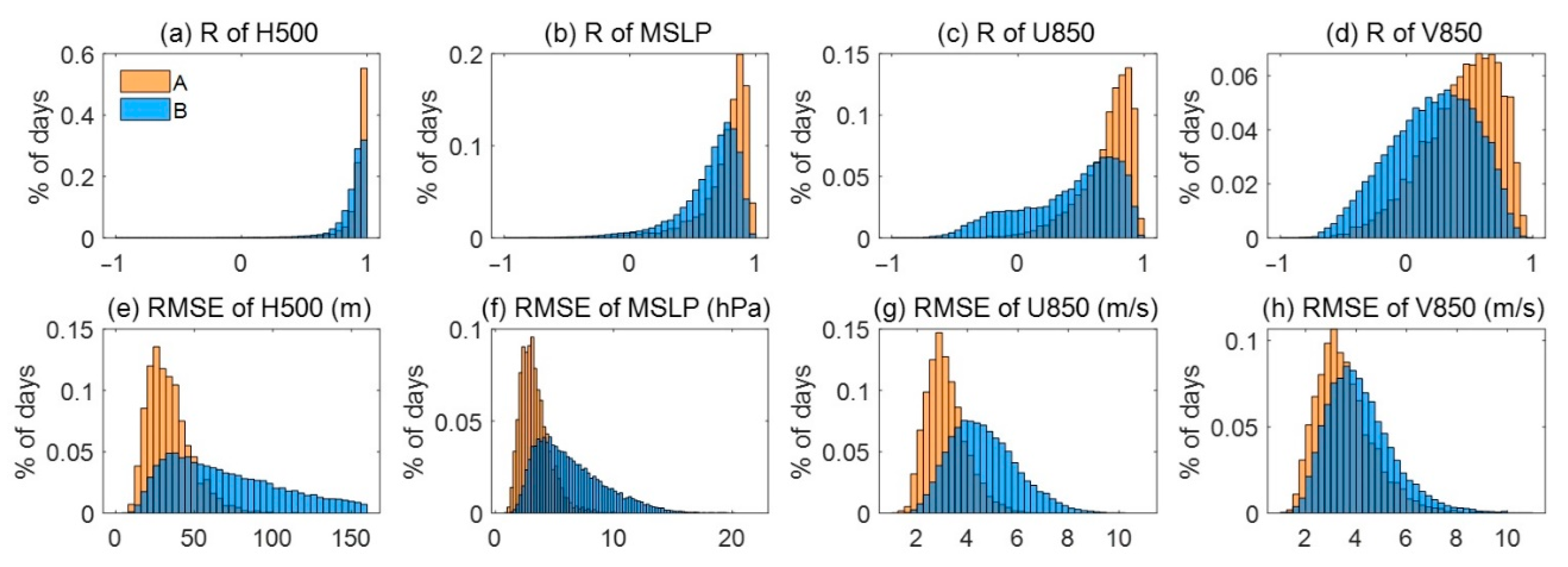
Figure 2 shows the calculated results of the R and RMSE analyses (histogram). The calculated results from the individual days and each type to which they were assigned is shown in yellow. The calculated results from the individual days and the types to which they were not assigned are shown in blue.
Between each individual day and the type to which they belong, a wide range of variations exist in the results of the calculations of the spatial correlation R for the four variable fields. For the different variables, the percentage of correlation coefficients greater than 0.5 that existed on the individual days and the types to which they belonged varied, being 98.6% (H500), 89.6% (MSLP), 84.1% (U850), and 47.2% (V850). Although the proportions of H500, MSLP, and U850 are all high; the lower proportion of V850 results in only about 40% of days when all four variables can have R greater than 0.5 at the same time. Between each individual day and the type to which they do not belong, the proportion of days with a correlation coefficient greater than 0.5 between the individual days and the category to which they belong differed from the different variables, being 97.3% (H500), 78.8% (MSLP), 50.9% (U850), and 22.1% (V850), respectively. However, the low percentage of U850 and V850 resulted in only 13.6% of days when the four variables could have R greater than 0.5 at the same time. The above results indicate that many days represented by the common state of the four variables can be represented by these types.
Similarly, the RMSE shows the affiliation minimum and the affiliation maximum. Between each individual day and the type to which they belong, the RMSE is generally smaller. Between each individual day and the type they do not belong to, the RMSE is generally larger.
In general, the highest R corresponds to the lowest RMSE. For H500, which is the variable field with the least spatial variation, the R is the highest and the RMSE is the lowest. The calculation results of the two wind field components are slightly poor. The above results show that it is reasonable and effective to use these two indicators to measure the quality of the clustering results.

3.1.2. Clustering Results

Before we go into any further analysis, the most basic thing to do was to identify a set of WTs to describe autumn weather in Southeastern China. In order to identify the WTs that can describe autumn weather in Southeastern China, we selected H500, MSLP, U850, and V850 of NCEP-2 reanalysis as the input data for SOM training. After SOM training, we obtained nine WTs.
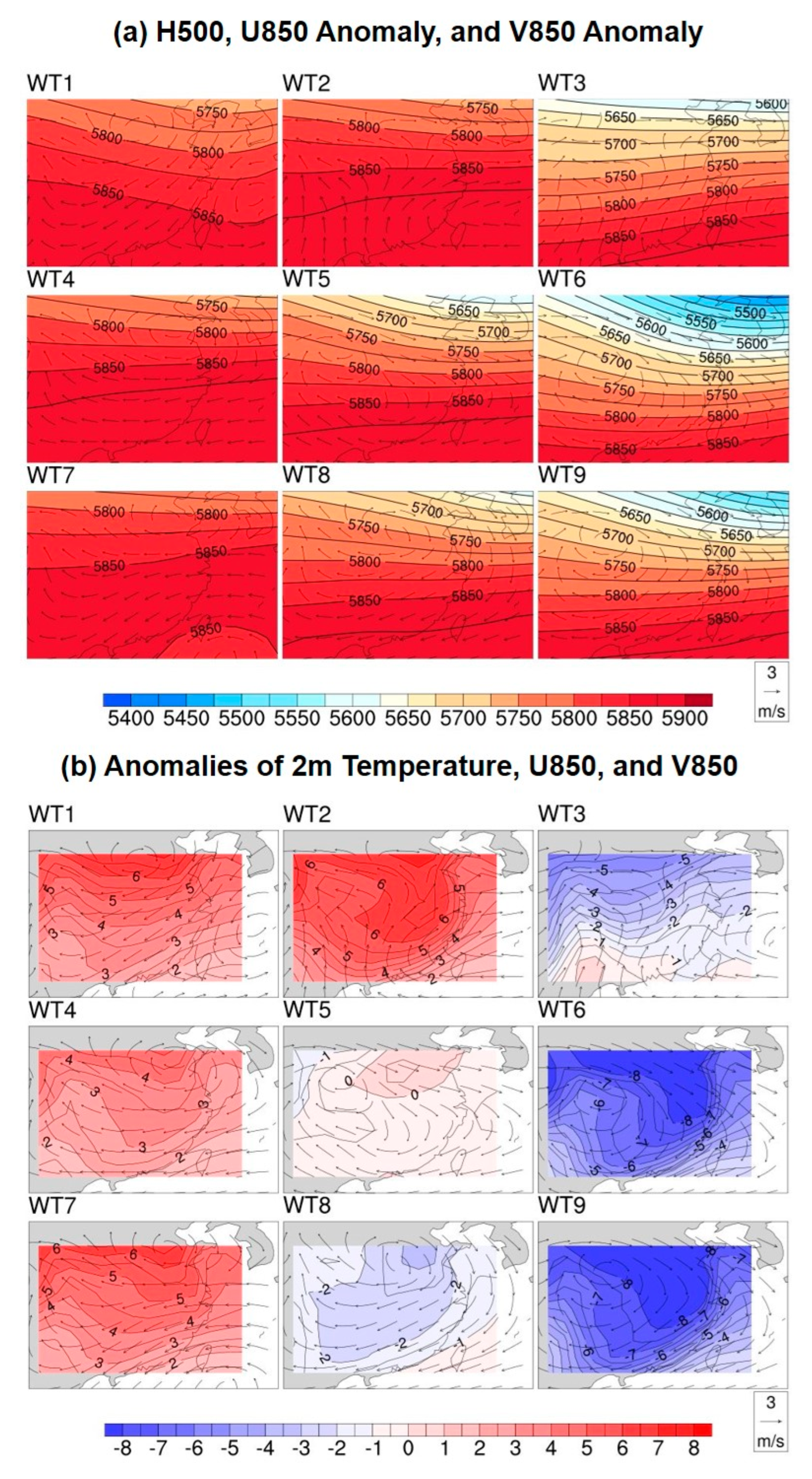
In order to display the SOM clustering results in detail, we plot MSLP and 850 hPa wind fields and H500 and 850 hPa wind fields, respectively, in Figure 3a,b. The temperature (2 m temperature) and precipitation corresponding to various WTs are, respectively, plotted in Figure 4a,b. The frequencies of all the WTs are 10.5%, 12.9%, 11.0%, 14.3%, 11.7%, 8.3%, 7.9%, 12.9%, and 10.4%, respectively. The frequency of occurrence of each weather type ranged from 7.9% (WT7) to 14.3% (WT4), with a mean value of 11.1%.
The distribution of the pressure distance-level field is similar for the neighboring weather patterns, and the distribution of the pressure distance-level field differs greatly for the distant weather patterns, which is mainly reflected in the strength and location differences of the high- and low-pressure systems. WT1, WT2, WT4, and WT7 are mainly dominated by trough, while WT9, WT8, and WT6 in the lower right corner and WT3 in the upper right corner differ greatly from the upper left corner, mainly dominated by high pressure. The middle WT5 is a transitional type with no obvious features.
In WT1, a trough is exhibited with higher land surface pressure, a low-pressure system from the southeastern ocean, the temperature and precipitation more than the average. On the one hand, low-pressure convergence tends to form updrafts. On the other hand, wind from the north and south directions converge in the region, which tends to bring sufficient rain. WT4 and WT7 are similar to WT1, except for the location and intensity of the fronts. WT2 has a different wind direction, with southerly winds prevailing and basically covering the whole region.
In WT9, a strong high-pressure system (Mongolian high pressure) is exhibited, with a high land surface pressure, and the high-pressure system comes from low-level winds from the northwest, with below-average temperatures and below-average precipitation over the whole area. In contrast to WT1, this type of high-pressure radiation dissipates, and sinking air flows are prevalent; on the other hand, there is no convergence of cold and warm air flows, and precipitation does not form easily. WT6 is similar to WT9. WT8 and WT3 are different in that the prevailing wind direction in these two types is different from WT9.

3.2. Temperature and Precipitation Distribution Characteristics in Each WT

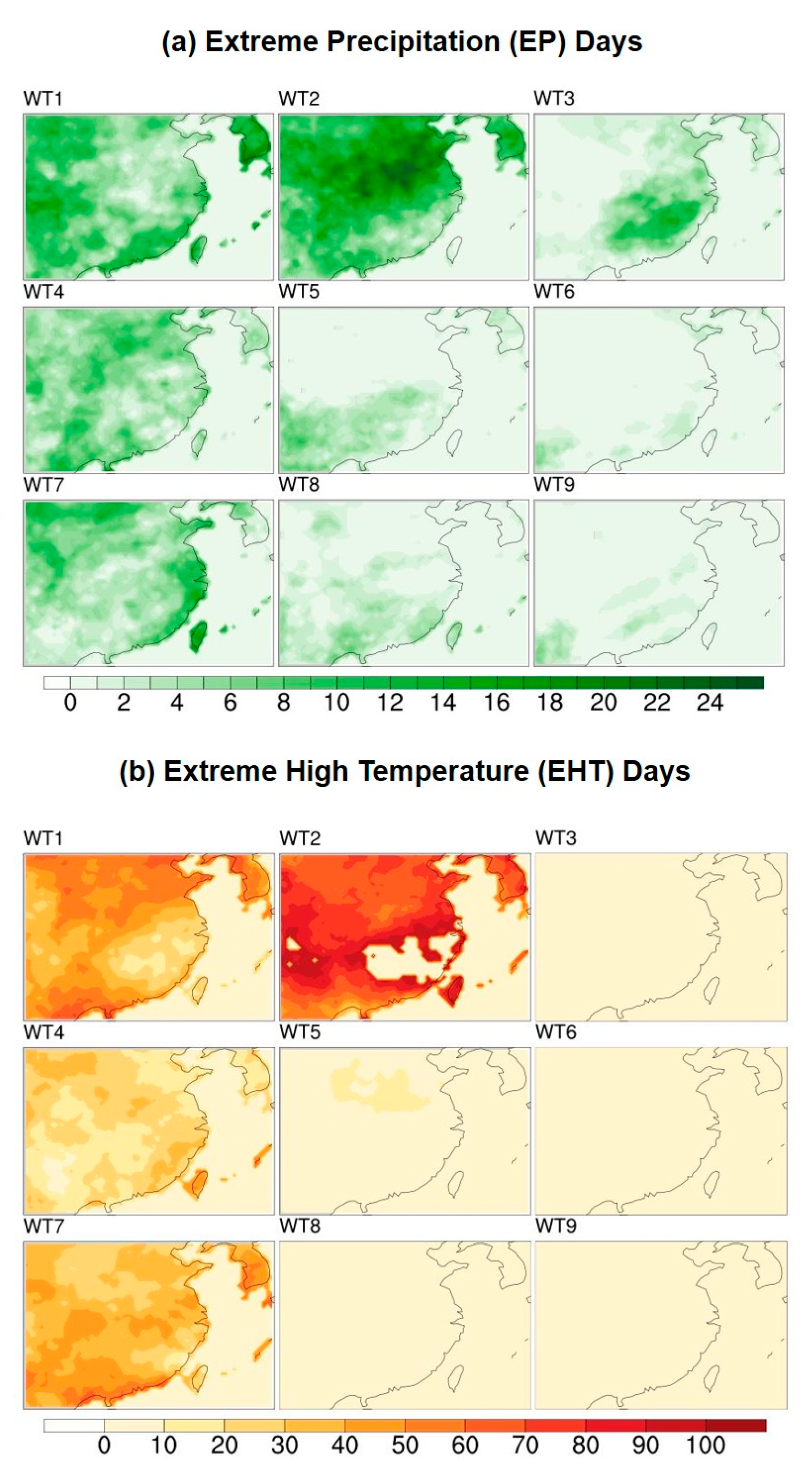
Temperature and precipitation are expressed in two forms, one in the form of the daily average distance level (Figure 3 and Figure 4) and the other in the case of extremes (Figure 5). EP is defined as precipitation above the 99th percentile of the grid point of any given day [70]. EHTs were analyzed for heat wave days. A heat wave day was defined as the highest grid point temperature above the 95th percentile [71].
For the average precipitation distance level (Figure 3a), WT1, WT7, and WT2 have the highest precipitation rates (3.7, 3.6, and 3.4 mm/day). WT6, WT9, and WT3 have the lowest precipitation rates (1.0, 1.1, and 1.3 mm/day). WT1, WT2, and WT7 have the largest positive precipitation anomalies, while WT3, WT6, and WT9 have the largest negative precipitation anomalies. WT1, WT7, and WT2 have positive precipitation anomalies over the entire region, spanning two-thirds of Southeastern China. The reason can be attributed to widespread and persistent frontal rain. WT6, WT9, and WT3 have mainly negative precipitation anomalies across the region. The cause can be attributed to the long-term control of Mongolian high pressure.
Regarding the average temperature of each WT (Figure 4), the hottest are WT1 and WT2, which appear early in the season. The coldest are WT9 and WT6, which appear late in the season.
For EP days, WT1 and WT2 contain the most (26% and 19%, respectively). EP is more likely to occur due to the occurrence of these two modes (Figure 5a), and EP is most likely to occur at inland grid points. WT1 is closer to the surrounding area, while WT2 is the whole area.
WT3, WT6, and WT9 have the least number of EP days (7%, 8%, and 1%, respectively). EP is less likely to occur when these patterns occur. Likewise, in these patterns, EP occurs mainly at coastal grid points. This depends on the location of the ridge.
Heat wave days mainly occur on WT1, WT2, WT4, and WT7. Among them, WT1 and WT2 are the most likely patterns of experiencing heat waves (Figure 5b). Heat wave days occur in most of the areas during the days experiencing WT1 and WT2. Heat wave days were rare in WT9, WT8, WT6, and WT3. Interestingly, although temperature variables are not considered in the clustering, the WT perspective view is able to capture the traditional heat wave patterns in Southeastern China (e.g., WT9 has strong ridges). This further confirms the SOM circulation-based WT clustering approach.

3.3. Teleconnection Relationship to WT Frequency

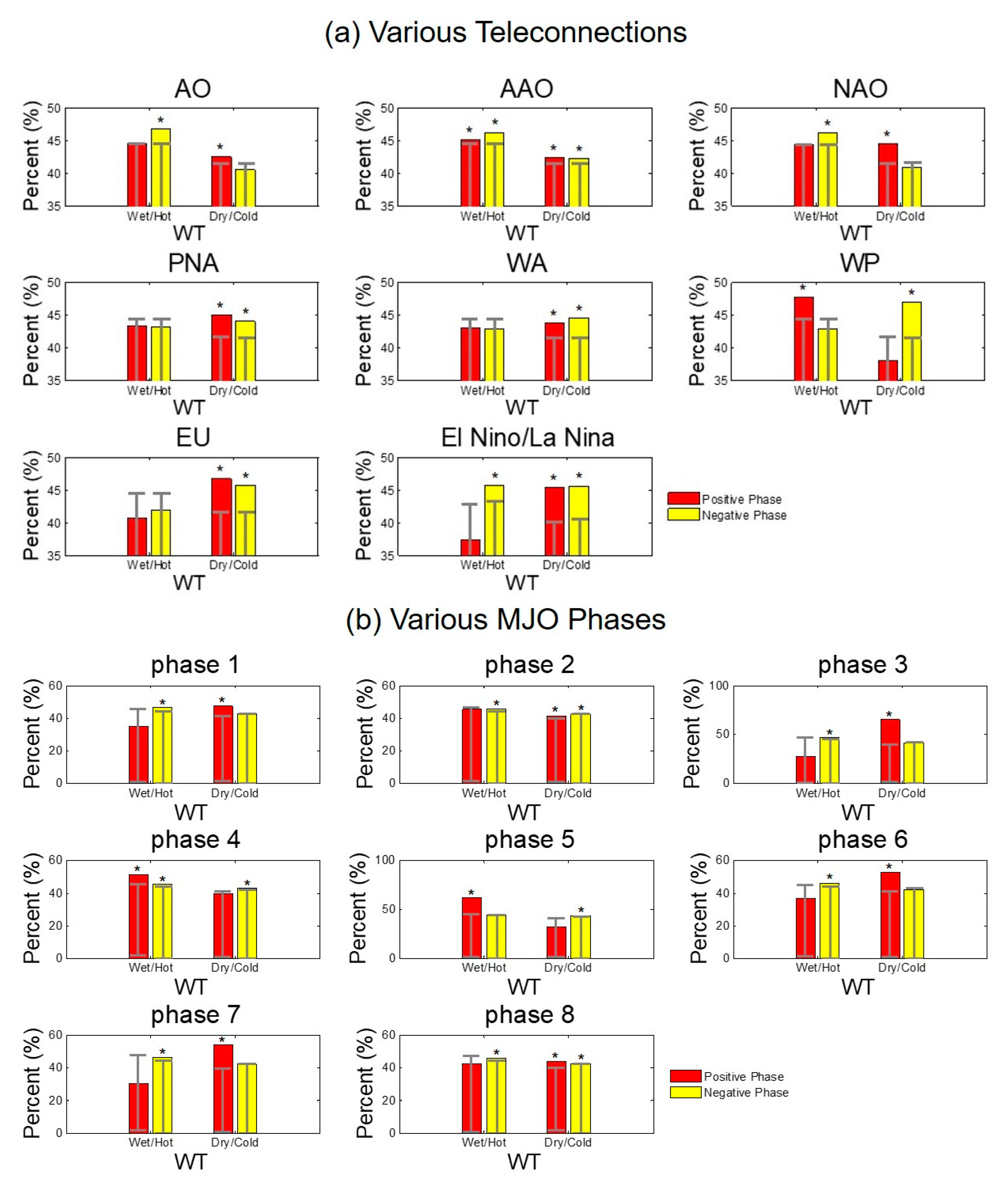
Perhaps there is an effect of various remotely correlated potential phase changes on the frequency variations of WTs [58]. For the qualitative analysis, we further merged the clustering results from two main categories: one is wet/hot (WT1, WT2, WT4, and WT7), which often occurs to the early fall (also called the early season pattern), has summer characteristics, and is prone to high temperatures and precipitation. The other category is the dry/cold (WT9, WT8, WT6, and WT3) pattern, which often occurs in the late fall (which can also be called the late season pattern) and possesses winter characteristics and is prone to causing low temperatures and droughts. In this way, the calculation results are clearer and more conducive to our qualitative analysis.
We selected several common atmospheric teleconnections. The main results are shown in Figure 6a. The monthly phase of El Niño/La Niña are also shown in Figure 6a. The threshold for the division of positive, neutral, and negative phases is [−1, 1], in which the neutral phases are neutral, greater than 1 are positive, and less than −1 are negative. Significance analysis was performed by the Monte Carlo method, and we did not care for all teleconnection neutral phases. Therefore, the results in the neutral phase are not shown. In addition, the MJO is also one of the important factors affecting the eastern part of China, and we analyzed the relationship between the eight different loci of the MJO and the WT frequency as well (as showed in Figure 6b).
In Figure 6a, we found that AO, AAO, and NAO have similar relationships with the WT frequency. This can be attributed to the close association with these three indicators [72]. Early season modalities (wet/hot) are more likely to occur in the negative phase (22% and 21% WT days) of the three indicators. Conversely, positive loci in two indicators are much less likely to occur (4% and 3%). The opposite also applies to the late season pattern (dry/cold) (5% and 8% for the negative phase and 15% and 13% for the positive phase). The early season pattern is typical of the negative phase circulation pattern of AO, AAO, and NAO, with a trough in Eastern China, below the mean H500. The temperatures are above average, and the precipitation is above average. Late season patterns have distinct positive phase features (AO, AAO, and NAO), accompanied by below-average precipitation and below-average air temperature. The correlation between PNA and WA is weaker than that of AO, AAO, and NAO (PNA has a similar pattern, while WA is the opposite). It may be because of their weaker correlation between the Chinese region.
It is important to note that the effect pattern is most pronounced for WP and EU. We can find that there is a law that different phases of WP and EU have opposite effects on the various patterns. That is, the same pattern corresponds to a positive (negative) phase of WP and a negative (positive) phase of EU. The pattern is reversed for the early season and late season patterns. In the positive (negative) phase of WP, the early (late) season patterns are often present. On the contrary, the late (early) season patterns occur frequently in the positive (negative) phase of EU.
WT frequencies were less correlated with ENSO than other teleconnections. Although all eight WTs are in phase with at least one ENSO locus of statistically significant changes (not shown), only one WT6 and WT9 have substantial but very insignificant changes. WT4 and WT8 are more likely to occur in a negative phase of ENSO (La Niña). When El Niño is in its positive phase, WT3 and WT5 are the two more common patterns. El Niño does not have a great impact on Eastern China. This less significant link between ÜWT frequencies is not surprising. Both the early season pattern and the late season pattern are likely to occur to both the positive and negative phases.
The relationship between the 8 bit phases of the MJO and WT frequencies is shown in Figure 6b. Among them, the fourth and fifth phases of the MJO are most likely to occur in the early season pattern, while the late season pattern is scattered among the remaining six phases of the MJO.

3.4. Progressions of Early and Late Season WTs

Differences between WTs throughout the fall were examined in the following forms: the monthly frequency, daily average evolution, and typical evolution. The evolution between WTs, individual WTs, and WTs was characterized in the early and late seasons based on the variations in frequency of occurrence over a 3-month-long season.

3.4.1. Monthly Frequency

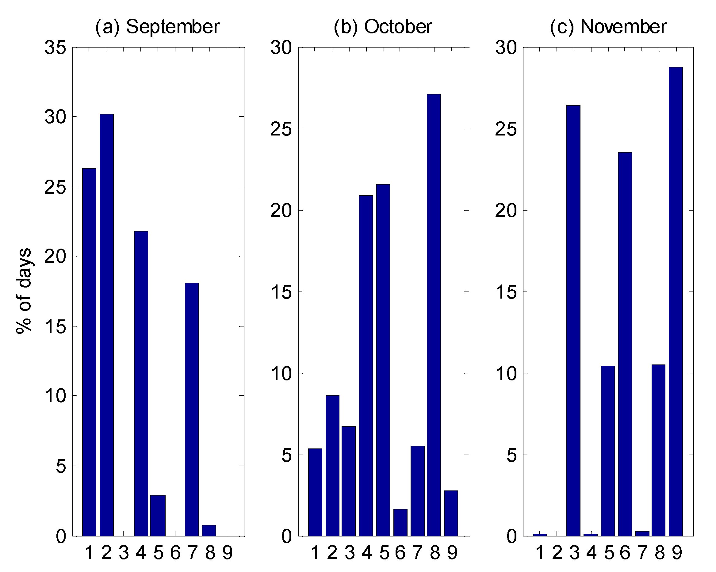
To measure the monthly rate of change of WT frequencies, monthly totals of WT frequencies were calculated for all years (Figure 7). On this basis, several WTs that occurred most frequently in each month were identified.
(1)
WT1, WT2, WT4, and WT7 in the month of September.
(2)
WT4, WT5, and WT8 in the month of October.
(3)
WT3, WT6, and WT9 in November.
WT2 and WT1 had the greatest incidence of decline. WT9, WT3, and WT6 had the largest rate of increase, from 0% in September to 28.8%, 26.4%, and 23.5% in November, respectively.

3.4.2. Daily Evolution

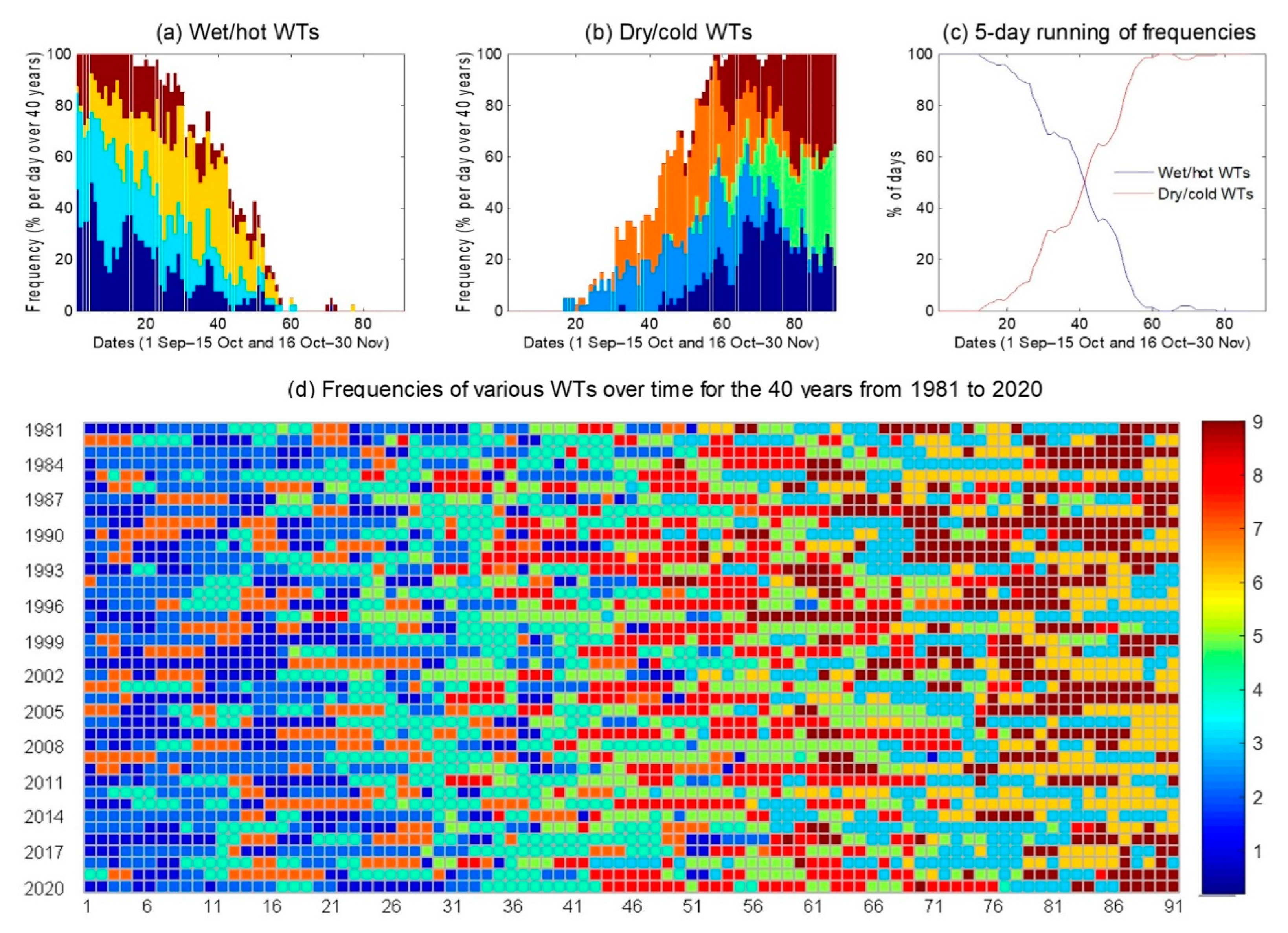
In order to more carefully observe the change of the occurrence frequency of each mode over all of autumn, we carried out a careful inspection, and the results are shown in Figure 8. All WTs are divided into two categories; one frequently appears in the early stage (Figure 8a), and the other frequently appears in the late stage (Figure 8b). Their respective trends are represented by their respective 5-day moving averages. The intersection of the two 5-day moving averages is considered to be the turning point of the trend (or the midpoint of autumn—specifically, 16 October). On this day, the probability of occurrence of the two types of WTs was equal at 50% (equal chance of occurrence.) October is a period of significant change, with dramatic changes in the frequency of occurrence of both types of WTs, the early and late season. Early season WTs often occur on days greater than 50% before October 16 and then rapidly drop to less than 25% of the remaining days of October, then less than 5% of the days in November (almost close to 0 at the latest). The frequency trend of the late season WTs shows that less than 5% of the days were in the early part of September, and greater than 50% of the days were in the late season after October 16. This pattern was evident throughout the 40-year period 1981–2020, with only slight variations in the specifics of each year (Figure 8d). The change of the early and late seasons is a gradual process, with no very clear cut-off point. A small fraction of late season WT also occurs before 16 October, and similarly, a small fraction of early season WT occurs after 16 October.

3.4.3. Typical Evolution

To further examine the development of WTs within seasons, we examined the WT progression (Table 1 and Table 2 and Figure 9). First, the dataset of the number of clusters was partitioned into a 40 × 91 matrix, with 40 representing 40 years and 91 representing a total of 91 days in the three months of autumn. Then, persistence was removed to enable counting the number of modalities. Those containing multiple consecutive class numbers (e.g., the forms “xyx” and “xxyyyxx” are equivalent) that occurred in each year with evolving numbers of lengths two, three, or four are counted. The sum of each year was also put together to obtain a total (Table 1). Note that, due to the length, only the top 10 results for each evolution are shown, while the evolution of lengths greater than four is not shown. This is because the highest counts of these evolutions are very few (less than 10) in the 40-year dataset.
From the table, we can find that, overall, the evolution appearing in the early season occupies the majority and has an absolute numerical advantage. In the evolution of length four, the first four are all early season, and only from the fifth place in the late season do modalities start to appear (3−8−9−6). Similarly, in the evolution of length three, the first five are all early season. In the evolution of length two, the top 10 are occupied by early season ones in 7 of the top 10. The above results indicate that inter-modal evolution is extremely common and frequent in the early autumn with a clear summer character. In contrast, modal evolution rarely occurred in the late autumn, and the evolutionary characteristics of the modalities are closer to those of the winter season.
Four frequently occurring evolutions of length four were found from September 1 to October 15 (Table 1). In the first half of the season, the four evolutions were specified as follows: 7−1−2−4 (E1), 4−7−1−2 (E2), 2−4−7−1 (E3), and 1−2−4−7 (E4). Late fall includes 3−8−9−6 (L1) and 5−3−8−9 (L2). Some subsets also appear frequently (Table 1). The most frequent occurrence of E1 in the early season was 13 times. The most frequent occurrence of L1 in the late season also occurred only seven times. In the evolution of length three and length two, the number of occurrences was significantly higher. For example, in the early season, the number of occurrences of 4−7−1 is 35, while the number of occurrences of 7−1 is 69. In the late season, although less frequent, a similar pattern is shown. For example, 8−5−3 appeared 18 times, and 8−5 appeared 65 times.
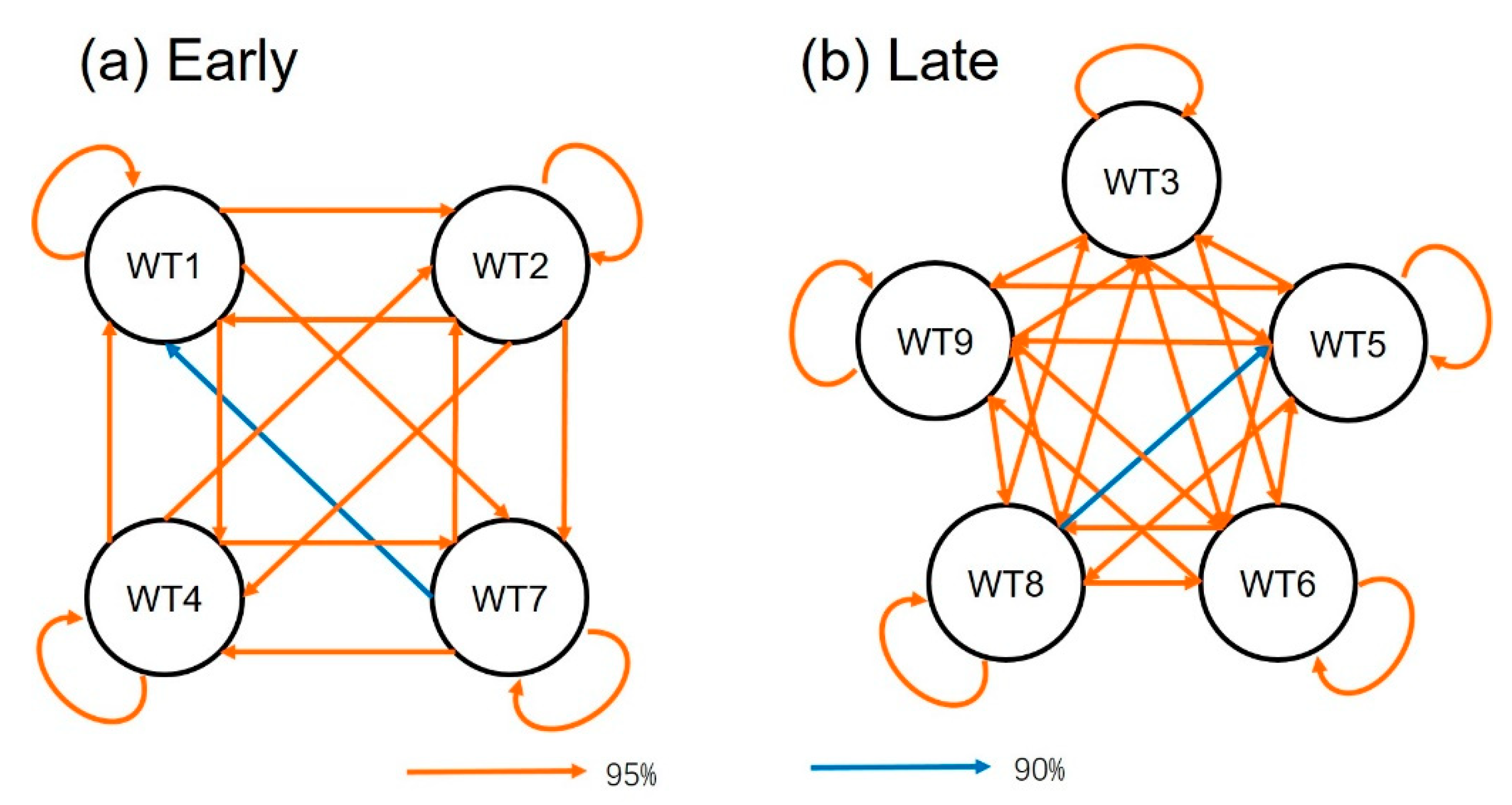
In the process of using Markov chains for analysis, a transition matrix is required. This was then run through a Monte Carlo method to find an evolution that made sense of the 95% confidence level. Initially, our analysis was built on the entire fall dataset. The evolutions “WT7−WT1” and “WT8−WT5” did not appear to be significant (at the 95% confidence level), although they occurred frequently (Table 1 and Figure 9). It is one of the features of this study to analyze and study the evolution of the alternating cold and warm autumn processes in the form of circulation modal transitions. The month-by-month analysis failed to capture this transition (not significant at the 95% level), so the entire fall season was analyzed by dividing it into two halves (1 September–15 October and 16 October–30 November). This could be seen at the 95% significance level (Table 2). We divided autumn into two parts on October 16 (Figure 8c, with a 50% probability of occurrence for both the early and late WT modes). It is reasonable to divide autumn into two halves in this way.
In Figure 9, we plotted the conversion relationships of the four WTs in the early season and the five WTs in the late season separately. The transitions to two of the various WTs are basically significant at the 95% level. Only individual transitions are significant at the 90% level (e.g., WT7−WT1 in Figure 9a and WT8−WT5 in Figure 9b).

3.4.4. Continuity of WT

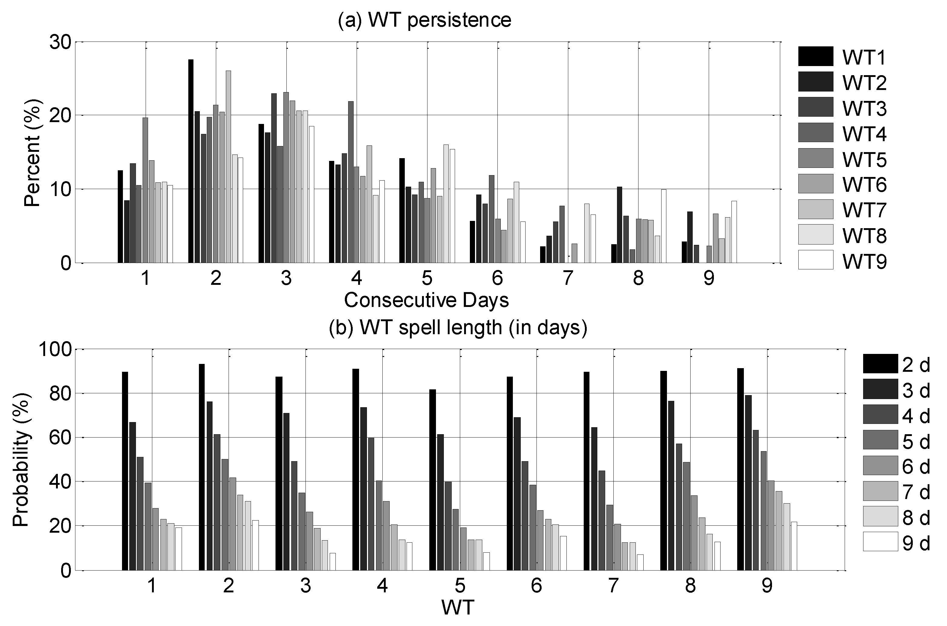
Persistence is shown in the clustering results as multiple consecutive occurrences of the same class number. From Figure 10a, it can be found that all WTs show the same pattern: the longer the duration days, the lower the frequency of occurrence. However, the ones with only 1 day of duration are not the ones with the highest proportion. It indicates that all kinds of patterns will have some persistence, but the duration is generally not too long. As can be seen in Figure 10b, the longer the duration, the lower the likelihood of occurrence of each type of WT. The proportion lasting 2 days is the highest, with most modalities lasting at least 2−3 days after their appearance. The proportion lasting 9 days is the lowest, and the proportion lasting more than 9 days is very low. It is unlikely that a particular modality will keep appearing continuously and will always switch to other modalities after a long period of time.

3.5. Characterization of Two Typical Progressions (One Representative from Each of the Front and Back Halves of the Fall)

The progressions of the WTs shown in Figure 11 and Figure 12 are synthesized from the days that occur in these evolutions. The synthetic fields of these modes have been redrawn for ease of observation. Evolutions between weather types reflect the movement of the weather system in the region. The more persistent they are, the slower they move (one weather type followed by the same weather type). The transition between patterns can be understood as a change in the troughs and ridges in the circulation field. This change can be manifested both as a change in the strengthening or weakening of the intensity and as a change in the position of the same circulating field as it appears in space.
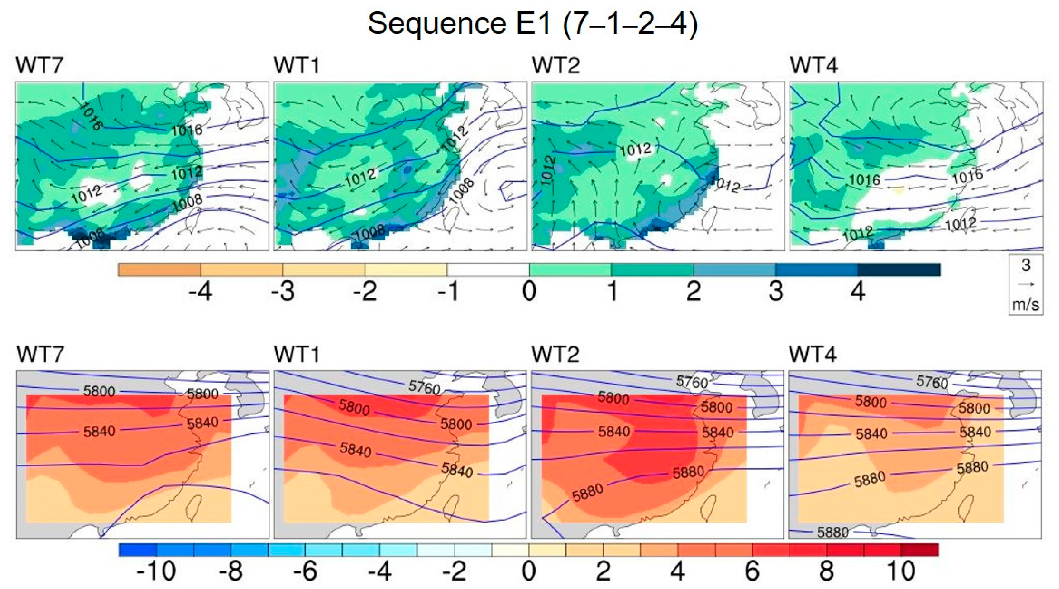
E1 is characterized by the convergence of high and low pressures here (Figure 11). This process causes the transition zone of two different natural air masses to fall in the southeastern part of China. It starts from WT7 and moves northward and eastward to WT2 and then retreats southwestward to WT4. This is a reciprocal movement. This process brings positive precipitation and positive temperature anomalies to the region. This is one of the wettest and warmest progressions, and the precipitation brought by this evolutionary process is extensive and persistent, because the fronts included in this process are large-scale weather systems in the coastal areas of Guangdong and Guangxi Provinces, where the highest anomalies were observed. Almost the whole region has above-average temperatures. Thus, this progression represents a shift in the circulation patterns and weather in the early season (the first half of autumn).
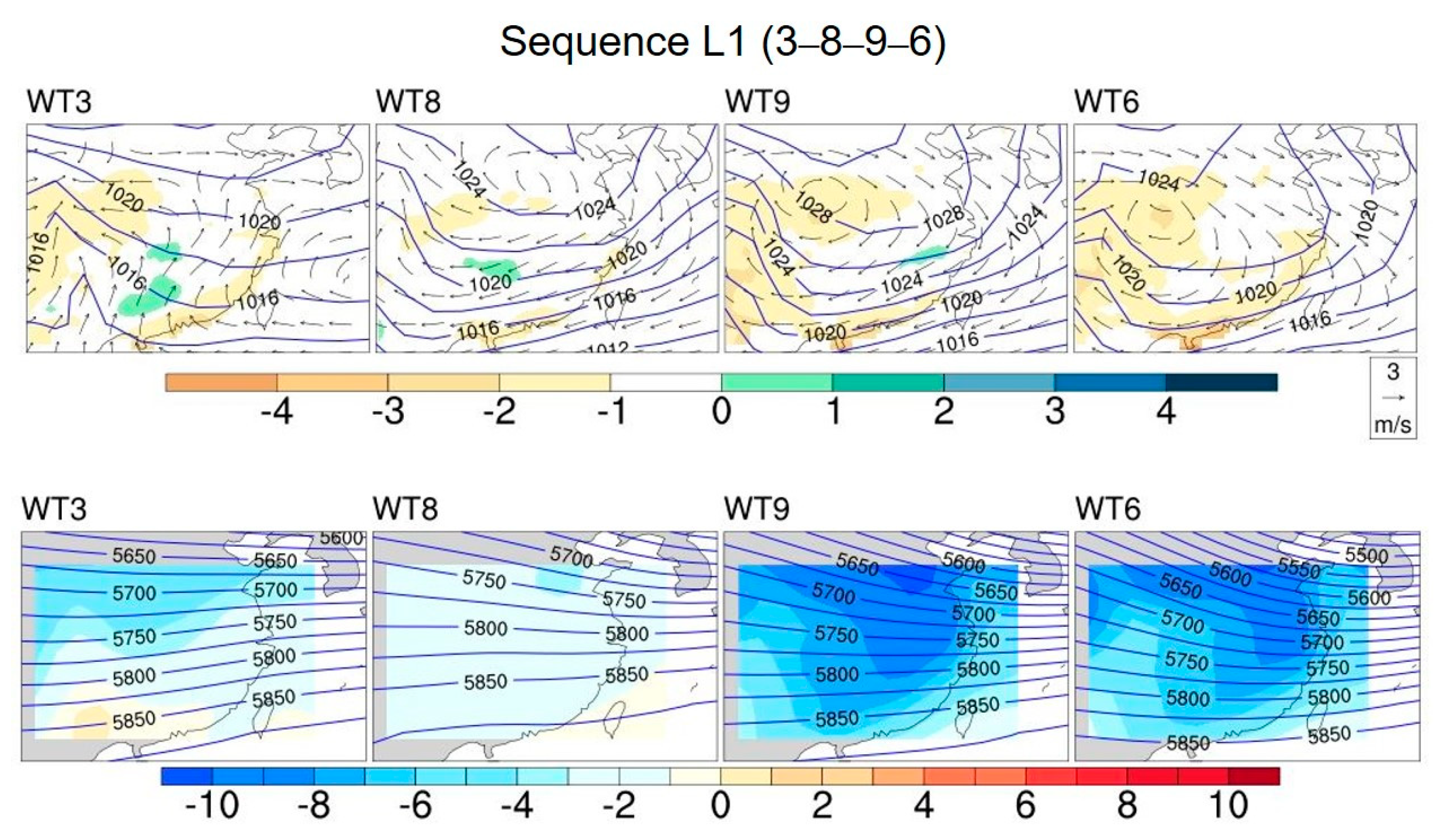
L1 is characterized by the southeastern part of China being controlled by the Mongolian high pressure (Figure 12). The circulation situation is characterized by a clockwise anticyclone. Its evolution is characterized by a process starting from WT3 that first intensifies, reaches its maximum strength at WT9, and then weakens (WT6). This leads to negative precipitation and temperature anomalies across Southeastern China, where dry and cold weather is prevalent, and several patterns are relatively similar. The change in the position of the high-pressure ridge is not very pronounced, but only the intensity alternates regularly in strength and weakness. Thus, this progression represents a shift in the circulation patterns and weather in the late season (second half of autumn).

3.6. Comparison of the Frequency of WT Occurrence in the Anterior and Posterior 20 Years of the Last 40 Years (1981–2020) between the Anterior and Posterior Halves of the Autumn

The clustering results provide a basis on which we can study the trend of seasonal variability in the form of daily circulation patterns for different periods. Differences in the occurrence frequency of the anterior and posterior seasons (between the anterior 20 and posterior 20 years of the 1981–2020 record) are considered.
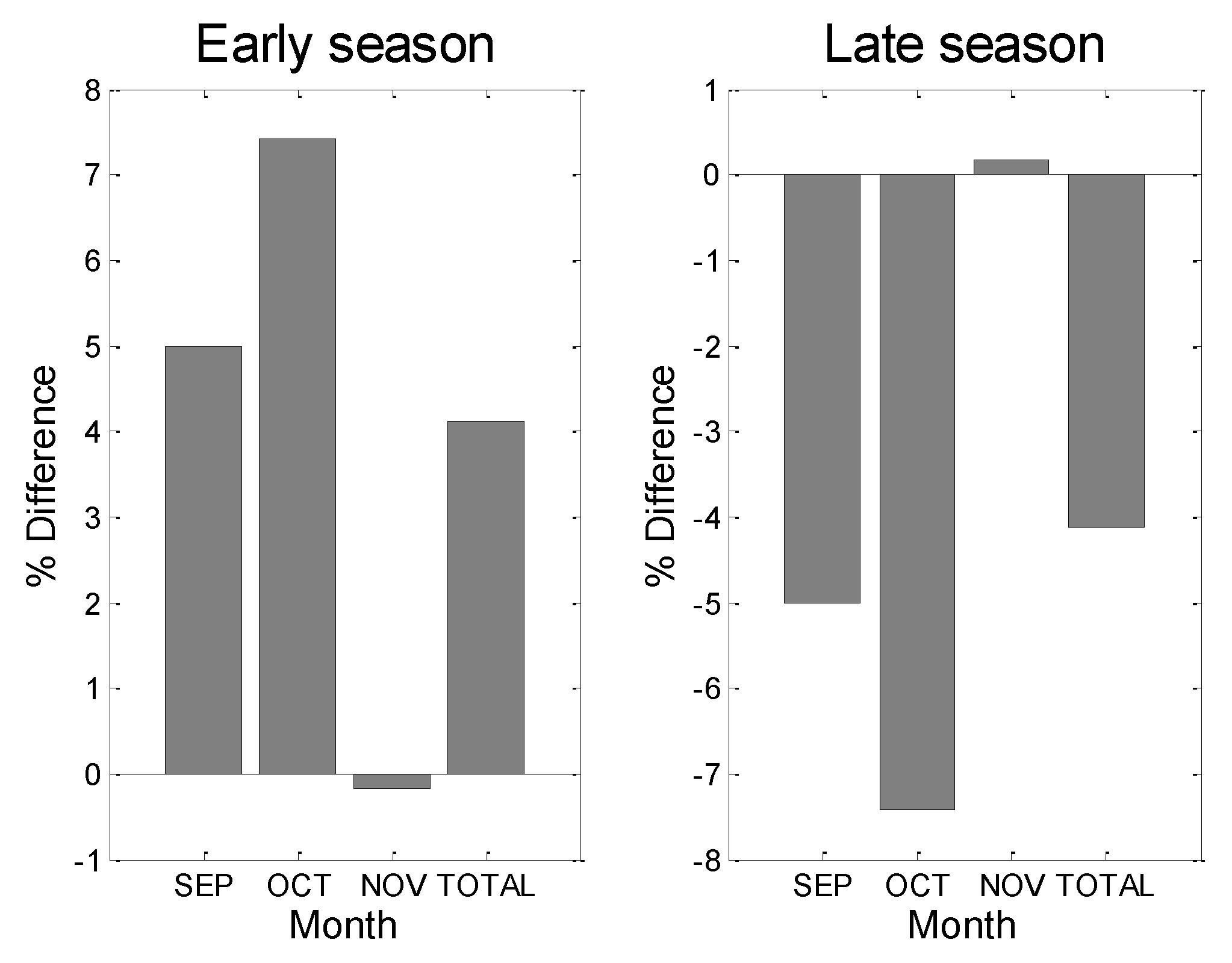
In Figure 13, the difference between the average monthly frequencies in the first and second halves of fall is plotted. In the first half of fall, the frequency increased significantly in the first two months and decreased slightly in the last month. In the second half of fall, the situation was completely opposite, with a significant decrease in the first two months and a slight increase in the last month. This result implies a clear interdecadal variation in the frequency of the circulation patterns. The warm and wet patterns are more frequent and persistent, while the dry and cold patterns are less frequent and occur later.
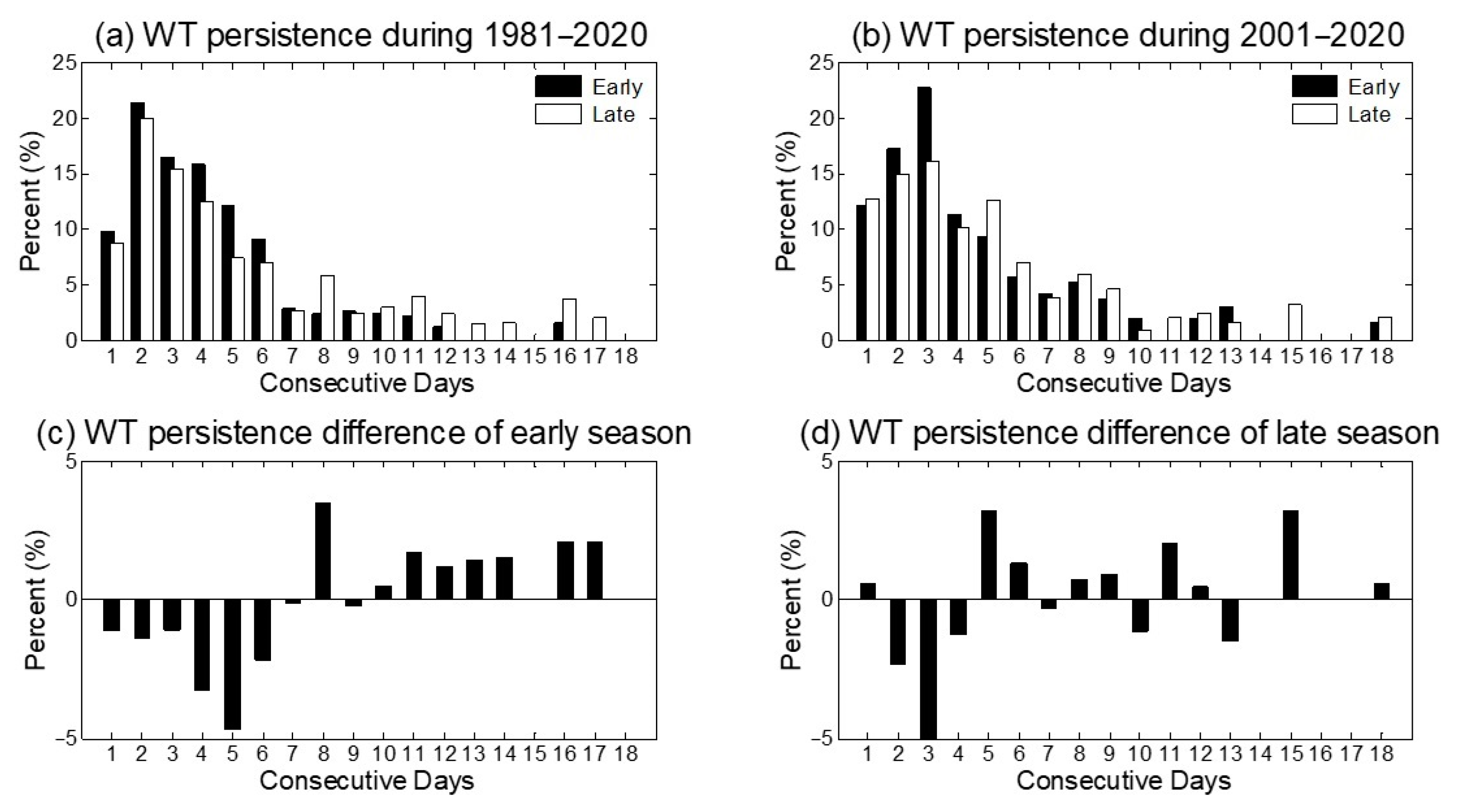
The change in the persistence of WTs within the two periods was further observed (Figure 14). Overall, the frequency of occurrence was higher for the shorter duration and lower for the longer duration of both periods. The highest frequency of occurrence in the period 1981–2000 was not for WTs of 1-day duration, but the highest frequency of occurrence of those of 2-days duration. Similarly, the most frequent occurrence in the period 2001–2020 was the one lasting 3 days, reflecting that the persistence of WT has intensified in the latter 20 years.
Next, we look at the difference in persistence of the two different patterns of the early and late seasons in the two preceding and following 20 years (Figure 14c,d). In general, the frequency of shorter persistence decreased, while the frequency of longer persistence increased. The specific performance of the two different patterns differed slightly from the early and late seasons. The frequency of occurrence of those with a duration of 7 days or less decreased significantly in the early season, and the frequency of occurrence of those with a duration of 8 days or more increased significantly. The frequency of those with a duration of less than 4 days decreased significantly in the late season, and the frequency of most of those with a duration of 5 days or more increased significantly. It reflects that the persistence of different types of patterns increased in the period 2001–2020. It means that the risk of occurrence of flooding and occurrence of drought are both on an increasing trend.

4. Summary and Discussion

By using the SOM clustering algorithm, nine different WTs were determined for daily time scales of Southeastern China during 1981–2020 using wind field information on NCEP2 data of four variables: 500 hPa geopotential high, MSLP, and 850 hPa zonal and meridional (u and v) component winds. The occurrence of WTs was analyzed for each month of the calendar. The results show that there are two different groups of WTs during the period 1981–2020. Four WTs (1, 2, 4, and 7) occurred more frequently in September than in November. Five WTs (3, 5, 6, 8, and 9) were more likely to occur in November than in September. These WTs showed a progression of priority to each other. The Markov chain analysis played an important role in our analysis. Applying this method, we successfully captured two different occurrence sequences that occurred in autumn. These two sequences represented the different weather characteristics in the early and late phases of autumn. The earlier sequence is closer to the summer season and is more likely to produce extreme weather. The late season weather is characterized by systems with longer single pattern durations and higher intensities, similar to winter weather characteristics. The analytical methods of the WTs also show some value in the analysis of extreme weather based on their relationship with standard teleconnection indices. Their seasonal variations are further discussed. The apparent seasonality of weather types on the daily scale of autumn shown here suggests that there may be additional value not only in terms of mean temperature [46].
In our clustering results, the closer the modalities are to each other, the more similar they are, and the more distant the modalities differ from each other. This is due to the characteristics of the SOM clustering method. Therefore, two sets of modes with opposite properties are located at the farthest distance, e.g., WT1 and WT9 are two modes with exactly opposite properties, and they are located at opposite ends of the diagonal. Among them, the modalities in the upper-left corner (WT1, WT2, and WT4) exhibit high temperatures and rainfall in nature and often occur in early autumn (early season pattern). In contrast to the upper-left corner, the lower-right patterns (WT9, WT8, WT6) are cold and dry in nature and often occur in late autumn (late season pattern). The middle WT5 is a transitional type of no distinct characteristics.
The early season pattern is clearly characterized by above-average surface temperatures and above-average precipitation. WT4 and WT7 are similar to WT1, except for the location and intensity of the fronts. WT2 has a different wind direction, with southerly winds prevailing and basically covering the entire region. The early season pattern is clearly characterized by below-average temperatures and below-average precipitation over the entire region. Represented by WT9, the land surface pressure is high and is controlled by the Mongolian high pressure. WT6 is similar to WT9. WT8 and WT3 are different in that the prevailing wind direction in these two categories is different from WT9.
Next, the incidence of EP and heat waves associated with WTs was analyzed. WT1 and WT2 contained the most, and WT3, WT6, and WT9 had the least number of EP days. EP can occur to any of the WTs, and the distribution of heat wave days is more dispersed. WT1, WT2, WT4, and WT7 cover most heat wave days, not WT3, WT6, WT8, and WT9. WT1 and WT2 have the most frequent heat wave days.
The relationship between AO, AAO, NAO, PNA, WA, WP, EU, ESNO, and MJO teleocorrelations and the frequency of WTs was examined next. The pattern of influence was the most evident for WP and EU, with the early season pattern (wet/hot) more likely to occur in the positive phase of WP, and the negative phase of the EU. AO, AAO, and NAO has similar relationships with the WT frequencies, and the wet/hot pattern is more likely to occur in the negative phase of all three atmospheric teleconnections. In addition, wet/hot patterns are most likely to occur to the fourth and fifth phases of the MJO, while dry/cold patterns are scattered among the remaining six phases of the MJO.
The transformation law between WTs can be analyzed by Markov chains. The transformation law shows a certain seasonality. Some progress occurs easily in the early autumn, while others occur frequently in the late season. The transformation between patterns is essentially a periodic change in the position and strength of the grooves and ridges. One of the most frequent early season evolutions (processes) contains four WTs (7, 1, 2, and 4). All four WTs are likely to occur in September, while they are very unlikely to occur in November. One of the most frequent late season evolutions also contains four WTs (3, 6, 8, and 9), in contrast to the early season; they are less likely to occur in September and more likely to occur in November. Something equally important to note is that each WT has the potential to transition back into itself the next day, i.e., for two days.
We compared the characteristics of two decades in the 40 years from 1981 to 2020. Patterns of the early season appear more frequently and last longer in the early season, and those in the late season appear less frequently and later. That is, the longer cool season pattern shifts to the shorter warm season mode. In addition, the persistence of both cool and warm types of patterns increased from 2001 to 2020 relative to 1981 to 2000, with an increasing trend in the risk of both the occurrence of floods and the occurrence of droughts. This suggests that the observed changes in temperature are associated with significant changes in the daily circulation in regional seasonal variations. This provides a new perspective in considering seasonal changes.
This study still does not fully address the problem, and there are still some questions that need to be further explored. For example, the frequency of weather patterns occurring in the early and late seasons has changed, and whether their internal structure also changes over time. This issue also needs to be further investigated.
The relationship between regional circulation patterns and large-scale circulation changes still needs to be further explored and studied. We plan to further address these outstanding questions in our future work. In addition, similar to autumn, spring is also a season of alternating warm and cold conditions. Our concerns include: what is the same or similar between spring and fall, what are the characteristics of the regional weather patterns in the spring, etc. What are the characteristics of changes of different modes throughout the year and whether the weather mode itself will change when the season changes; these issues are to be discussed in our next work. For the prediction of future climate scenarios, we also hope that these findings will be applied and can be successfully extended to the rest of the world.

Author Contributions

Conceptualization, Y.W.; project administration, Y.W.; supervision, X.S.; validation, Y.W.; writing–original draft, X.S.; and writing—review and editing, Y.W. All authors have read and agreed to the published version of the manuscript.

Funding

This research was funded by the China Postdoctoral Science Foundation, Grant No. 2018M632334.

Institutional Review Board Statement

Not applicable.

Informed Consent Statement

Not applicable.

Data Availability Statement

The codes and datasets generated during and/or analyzed during the current study are available from the corresponding author on reasonable request. The National Center for Environmental Prediction (NCEP)-U.S. Department of Energy (DOE) AMIP-II (NCEP-2) reanalysis of daily gridded atmospheric data were used. This set of data was provided by the NOAA PSL, Boulder, CO, USA (https://psl.noaa.gov, accessed on 10 August 2021) and the NOAA Climate Prediction Center (CPC; https://psl.noaa.gov/data/gridded/data.cpc.globalprecip.html, accessed on 10 August 2021). The MJO index developed by Wheeler et al. can be downloaded from the Australia Meteorological Bureau (http://www.bom.gov.au/climate/mjo/, accessed on 10 August 2021). The monthly Niño-3.4 index was obtained from the Climate Prediction Center (https://www.cpc.ncep.noaa.gov/products/precip/CWlink/daily_ao_index/teleconnections.shtml, accessed on 10 August 2021).

Acknowledgments

We acknowledge the National Center for Environmental Prediction (NCEP)-U.S. Department of Energy (DOE) AMIP-II (NCEP-2) reanalysis of daily gridded atmospheric data we used. This set of data was provided by the NOAA PSL, Boulder, CO, USA (https://psl.noaa.gov, accessed on 10 August 2021). We acknowledge the NOAA Climate Prediction Center (CPC; https://psl.noaa.gov/data/gridded/data.cpc.globalprecip.html, accessed on 10 August 2021). We acknowledge the MJO index developed by Wheeler et al. that can be downloaded from the Australia Meteorological Bureau (http://www.bom.gov.au/climate/mjo/, accessed on 10 August 2021). The monthly Niño-3.4 index was obtained from the Climate Prediction Center (https://www.cpc.ncep.noaa.gov/products/precip/CWlink/daily_ao_index/teleconnections.shtml, accessed on 10 August 2021). We acknowledge the helpful comments of three anonymous reviewers and the editor, who helped in improving this manuscript.

Conflicts of Interest

The authors declare no conflict of interest. The funders had no role in the design of the study; in the collection, analyses, or interpretation of the data; in the writing of the manuscript; or in the decision to publish the results.

References

  1. Liu, K. The Variation of Autumn Rainfall in Southeast China and Its Association with Sea Surface Temperature in the Tropical Pacifil Sea. Ph.D. Thesis, Yunnan University, Kunming, China, 2018. [Google Scholar]
  2. Jian, M.Q.; Qiao, Y.T. Characteristics of general circulation anomalies related to the drought events in fall in south China. Chin. J. Atmos. Sci. 2012, 36, 204–214. [Google Scholar]
  3. Jiang, Z.Y.; Xu, H.M.; Ma, J. Atmospheric circulation characteristics of heavy precipitation events and impact of sea surface temperature over the southern China in the autumn of 2016. Chin. J. Atmos. Sci. 2021, 45, 1023–1038. (In Chinese) [Google Scholar] [CrossRef]
  4. Sha, T.Y.; Xu, H.M.; Zou, S.Z. Atmospheric circulation characteristics and cause analysis for autumn drought in the eastern region of southwest China. Trans. Atmos. Sci. 2013, 36, 593–603. (In Chinese) [Google Scholar] [CrossRef]
  5. Ohba, M.; Ueda, H. A role of zonal gradient of SST between the Indian ocean and the western pacific in localized convection around the Philippines. SOLA 2006, 2, 176–179. [Google Scholar] [CrossRef] [Green Version]
  6. Xie, S.-P.; Hu, K.; Hafner, J.; Tokinaga, H.; Du, Y.; Huang, G.; Sampe, T. Indian ocean capacitor effect on Indo—Western pacific climate during the summer following El Niño. J. Clim. 2009, 22, 730–747. [Google Scholar] [CrossRef]
  7. Kosaka, Y.; Xie, S.-P.; Lau, N.-C.; Vecchi, G.A. Origin of seasonal predictability for summer climate over the northwestern Pacific. Proc. Natl. Acad. Sci. USA 2013, 110, 7574–7579. [Google Scholar] [CrossRef] [Green Version]
  8. Du, Y.; Yang, L.; Xie, S.-P. Tropical Indian ocean influence on northwest pacific tropical cyclones in summer following strong El Niño. J. Clim. 2011, 24, 315–322. [Google Scholar] [CrossRef]
  9. Yonekura, E.; Hall, T.M. ENSO effect on east Asian tropical cyclone landfall via changes in tracks and genesis in a statistical model. J. Appl. Meteorol. Clim. 2014, 53, 406–420. [Google Scholar] [CrossRef] [Green Version]
  10. Wu, R.; Hu, Z.Z.; Kirtman, B.P. Evolution of ENSO-related rainfall anomalies in east Asia. J. Clim. 2003, 16, 3742–3758. [Google Scholar] [CrossRef]
  11. Yamaura, T.; Tomita, T. Covariability between the baiu precipitation and tropical cyclone activity through large-scale atmospheric circulations. J. Meteorol. Soc. Jpn. 2012, 90, 449–465. [Google Scholar] [CrossRef] [Green Version]
  12. El-Kadi, A.K.A.; Smithson, P.A. Atmospheric classifications and synoptic climatology. Prog. Phys. Geogr. 1992, 16, 432–455. [Google Scholar] [CrossRef]
  13. Huth, R.; Beck, C.; Philipp, A.; Demuzere, M.; Ustrnul, Z.; Cahynová, M.; Kyselý, J.; Tveito, O.E. Classifications of atmospheric circulation patterns. Ann. N. Y. Acad. Sci. 2008, 1146, 105–152. [Google Scholar] [CrossRef]
  14. Ramos, A.M.; Barriopedro, D.; Dutra, E. Circulation weather types as a tool in atmospheric, climate, and environmental research. Front. Environ. Sci. 2015, 3, 44. [Google Scholar] [CrossRef] [Green Version]
  15. Muñoz, Á.G.; Yang, X.; Vecchi, G.A.; Robertson, A.W.; Cooke, W.F. A weather-type-based cross-time-scale diagnostic framework for coupled circulation models. J. Clim. 2017, 30, 8951–8972. [Google Scholar] [CrossRef]
  16. Kang, I.-S.; Ho, C.-H.; Lim, Y.-K. Principal modes of climatological seasonal and intraseasonal variations of the asian summer monsoon. Mon. Weather Rev. 1999, 127, 322–340. [Google Scholar] [CrossRef]
  17. Lau, K.-M.; Chan, P.H. Aspects of the 40–50 day oscillation during the northern summer as inferred from outgoing longwave radiation. Mon. Weather Rev. 1986, 114, 1354–1367. [Google Scholar] [CrossRef]
  18. Krishnamurthy, V.; Shukla, J. Intraseasonal and seasonally persisting patterns of Indian monsoon rainfall. J. Clim. 2007, 20, 3–20. [Google Scholar] [CrossRef] [Green Version]
  19. Yoo, J.H.; Robertson, A.W.; Kang, I.-S. Analysis of intraseasonal and interannual variability of the asian summer monsoon using a hidden Markov model. J. Clim. 2010, 23, 5498–5516. [Google Scholar] [CrossRef]
  20. Kohonen, T. Self-organized formation of topologically correct feature maps. Biol. Cybern. 1982, 43, 59–69. [Google Scholar] [CrossRef]
  21. Ohba, M.; Kadokura, S.; Yoshida, Y.; Nohara, D.; Toyoda, Y. Anomalous weather patterns in relation to heavy precipitation events in Japan during the baiu season. J. Hydrometeorol. 2015, 16, 688–701. [Google Scholar] [CrossRef]
  22. Hewitson, B.C.; Crane, R.G. Self-organizing maps: Applications to synoptic climatology. Clim. Res. 2002, 22, 13–26. [Google Scholar] [CrossRef]
  23. Reusch, D.B.; Hewitson, B.C.; Alley, R.B. Towards ice-core-based synoptic reconstructions of west antarctic climate with artificial neural networks. Int. J. Clim. 2005, 25, 581–610. [Google Scholar] [CrossRef]
  24. Hope, P.K.; Drosdowsky, W.; Nicholls, N. Shifts in the synoptic systems influencing southwest western Australia. Clim. Dyn. 2006, 26, 751–764. [Google Scholar] [CrossRef]
  25. Verdon-Kidd, D.C.; Kiem, A.S. On the relationship between large-scale climate modes and regional synoptic patterns that drive Victorian rainfall. Hydrol. Earth Syst. Sci. 2009, 13, 467–479. [Google Scholar] [CrossRef] [Green Version]
  26. Reusch, D.B. Nonlinear climatology and paleoclimatology: Capturing patterns of variability and change with self-organizing maps. Phys. Chem. Earth Parts A/B/C 2010, 35, 329–340. [Google Scholar] [CrossRef]
  27. Hosking, J.S.; Fogt, R.; Thomas, E.R.; Moosavi, V.; Phillips, T.; Coggins, J.; Reusch, D. Accumulation in coastal west Antarctic ice core records and the role of cyclone activity. Geophys. Res. Lett. 2017, 44, 9084–9092. [Google Scholar] [CrossRef] [Green Version]
  28. Leloup, J.A.; Lachkar, Z.; Boulanger, J.-P.; Thiria, S. Detecting decadal changes in ENSO using neural networks. Clim. Dyn. 2007, 28, 147–162. [Google Scholar] [CrossRef]
  29. Tozuka, T.; Luo, J.-J.; Masson, S.; Yamagata, T. Tropical Indian ocean variability revealed by self-organizing maps. Clim. Dyn. 2008, 31, 333–343. [Google Scholar] [CrossRef]
  30. Johnson, N.C. How many ENSO flavors can we distinguish? J. Clim. 2013, 26, 4816–4827. [Google Scholar] [CrossRef]
  31. Reusch, D.B.; Alley, R.B.; Hewitson, B.C. North Atlantic climate variability from a self-organizing map perspective. J. Geophys. Res. Earth Surf. 2017, 112, 7460. [Google Scholar] [CrossRef]
  32. Johnson, N.C.; Feldstein, S.B. The continuum of north Pacific sea level pressure patterns: Intraseasonal, interannual, and interdecadal variability. J. Clim. 2010, 23, 851–867. [Google Scholar] [CrossRef] [Green Version]
  33. Kolczynski, W.C.; Hacker, J.P. The potential for self-organizing maps to identify model error structures. Mon. Weather Rev. 2014, 142, 1688–1696. [Google Scholar] [CrossRef]
  34. Radić, V.; Clarke, G. Evaluation of IPCC models’ performance in simulating late-twentieth-century climatologies and weather patterns over north America. J. Clim. 2011, 24, 5257–5274. [Google Scholar] [CrossRef] [Green Version]
  35. Cavazos, T.; Comrie, A.C.; Liverman, D.M. Intraseasonal variability associated with wet monsoons in southeast Arizona. J. Clim. 2002, 15, 2477–2490. [Google Scholar] [CrossRef]
  36. Chattopadhyay, R.; Sahai, A.K.; Goswami, B.N. Objective identification of nonlinear convectively coupled phases of monsoon intraseasonal oscillation: Implications for prediction. J. Atmos. Sci. 2008, 65, 1549–1569. [Google Scholar] [CrossRef]
  37. Chu, J.-E.; Hameed, S.N.; Ha, K.-J. Nonlinear, intraseasonal phases of the east asian summer monsoon: Extraction and analysis using self-organizing maps. J. Clim. 2012, 25, 6975–6988. [Google Scholar] [CrossRef] [Green Version]
  38. Cavazos, T. Large-scale circulation anomalies conducive to extreme precipitation events and deviation of daily rainfall in northeastern Mexico and southeastern Texas. J. Clim. 1999, 12, 1506–1523. [Google Scholar] [CrossRef]
  39. Nishiyama, K.; Endo, S.; Jinno, K.; Uvo, C.B.; Olsson, J.; Berndtsson, R. Identification of typical synoptic patterns causing heavy rainfall in the rainy season in Japan by a self-organizing map. Atmos. Res. 2007, 83, 185–200. [Google Scholar] [CrossRef]
  40. Cassano, J.; Uotila, P.; Lynch, A.H.; Cassano, E.N. Predicted changes in synoptic forcing of net precipitation in large Arctic river basins during the 21st century. J. Geophys. Res. Earth Surf. 2007, 112, 332. [Google Scholar] [CrossRef] [Green Version]
  41. Polo, I.; Ullmann, A.; Roucou, P.; Fontaine, B. Weather regimes in the euro-atlantic and mediterranean sector, and relationship with west African rainfall over the 1989–2008 period from a self-organizing maps approach. J. Clim. 2011, 24, 3423–3432. [Google Scholar] [CrossRef] [Green Version]
  42. Cassano, J.J.; Uotila, P.; Lynch, A. Changes in synoptic weather patterns in the polar regions in the twentieth and twenty-first centuries, part 1: Arctic. Int. J. Clim. 2006, 26, 1027–1049. [Google Scholar] [CrossRef]
  43. Lee, C.C. The development of a gridded weather typing classification scheme. Int. J. Clim. 2015, 35, 641–659. [Google Scholar] [CrossRef] [Green Version]
  44. Easterling, D.R. Recent changes in frost days and the frost-free season in the United States. Bull. Am. Meteorol. Soc. 2002, 83, 1327–1332. [Google Scholar] [CrossRef]
  45. Cooter, E.J.; Leduc, S.K. Recent frost date trends in the north-eastern USA. Int. J. Clim. 1995, 15, 65–75. [Google Scholar] [CrossRef]
  46. Trenberth, K.E. What are the seasons? Bull. Am. Meteorol. Soc. 1983, 64, 1276–1282. [Google Scholar] [CrossRef]
  47. Sheridan, S.C. The redevelopment of a weather-type classification scheme for north America. Int. J. Clim. 2002, 22, 51–68. [Google Scholar] [CrossRef]
  48. Fleming, E.L.; Lim, G.; Wallace, J.M. 1987: Differences between the spring and autumn circulation of the northern hemi-sphere. J. Atmos. Sci. 1987, 44, 1266–1286. [Google Scholar] [CrossRef]
  49. Allen, M.J.; Sheridan, S.C. Evaluating changes in season length, onset, and end dates across the United States (1948–2012). Int. J. Clim. 2016, 36, 1268–1277. [Google Scholar] [CrossRef]
  50. Park, B.-J.; Kim, Y.-H.; Min, S.-K.; Lim, E.-P. Anthropogenic and natural contributions to the lengthening of the summer season in the northern hemisphere. J. Clim. 2018, 31, 6803–6819. [Google Scholar] [CrossRef]
  51. Meseguer-Ruiz, O.; Cortesi, N.; Guijarro, J.A.; Sarricolea, P. Weather regimes linked to daily precipitation anomalies in Northern Chile. Atmos. Res. 2019, 236, 104802. [Google Scholar] [CrossRef]
  52. Niu, N.; Li, J.P. The features of the heavy drought occurring to the south of the Yangtze River in China as well as the anomalies of atmospheric circulation in autumn 2004. Chin. J. Atmos. Sci. 2007, 31, 255–264. (In Chinese) [Google Scholar]
  53. Wang, Z.Y.; Zhou, B.T. Observed decadal transition in trend of autumn rainfall over central China in the late 1990s. J. Clim. 2019, 32, 1395–1409. [Google Scholar] [CrossRef]
  54. Gong, D.Y.; Wang, S.W. Impact of ENSO on global land and precipitation in China in the last 100 years. Chin. Sci. Bull. 1999, 44, 315–320. (In Chinese) [Google Scholar] [CrossRef]
  55. Zhou, B.T.; Xu, M.L.; Sun, B.; Han, T.T.; Cheng, Z.G. Possible role of southern hemispheric sea ice in the variability of west China autumn rain. Atmos. Res. 2021, 249, 105329. [Google Scholar] [CrossRef]
  56. Zhu, J.X.; Huang, G.; Wang, X.Q.; Cheng, G.H. Investigation of changes in extreme temperature and humidity over China through a dynamical downscaling approach. Earth’s Futur. 2017, 5, 1136–1155. [Google Scholar] [CrossRef]
  57. Roller, C.D.; Qian, J.-H.; Agel, L.; Barlow, M.; Moron, V. Winter weather regimes in the northeast United States. J. Clim. 2016, 29, 2963–2980. [Google Scholar] [CrossRef]
  58. Coe, D.; Barlow, M.; Agel, L.; Colby, F.; Skinner, C.; Qian, J.-H. Clustering analysis of autumn weather regimes in the northeast United States. J. Clim. 2021, 34, 7587–7605. [Google Scholar] [CrossRef]
  59. Wallace, J.M.; Gutzler, D.S. Teleconnections in the geopotential height field during the northern hemisphere winter. Mon. Weather Rev. 1981, 109, 784–812. [Google Scholar] [CrossRef]
  60. Thompson, D.W.J.; Wallace, J.M. The arctic oscillation signature in the wintertime geopotential height and temperature fields. Geophys. Res. Lett. 1998, 25, 1297–1300. [Google Scholar] [CrossRef] [Green Version]
  61. Thompson, D.W.J.; Wallace, J.M. Annular modes in the extratropical circulation. Part I: Month-to-month variability. J. Climate. 2000, 13, 1000–1016. [Google Scholar] [CrossRef]
  62. Wheeler, M.C.; Hendon, H.H. An all-season real-time multivariate MJO index: Development of an index for monitoring and prediction. Mon. Weather Rev. 2004, 132, 1917–1932. [Google Scholar] [CrossRef]
  63. Bjerknes, J. Atmospheric teleconnections from the equatorial Pacific. Mon. Wea. Rev. 1969, 97, 163–172. [Google Scholar] [CrossRef]
  64. Kanamitsu, M.; Ebisuzaki, W.; Woollen, J.; Yang, S.K.; Hnilo, J.J.; Fiorino, M.; Potter, G.L. NCEP–DOE AMIP-II reanalysis (R-2). Bull. Am. Meteorol. Soc. 2002, 83, 1631–1643. [Google Scholar] [CrossRef] [Green Version]
  65. Reynolds, R.W.; Rayner, N.A.; Smith, T.M.; Stokes, D.C.; Wang, W. An improved in situ and satellite SST analysis for climate. J. Clim. 2002, 15, 1609–1625. [Google Scholar] [CrossRef]
  66. Richardson, A.; Risien, C.; Shillington, F. Using self-organizing maps to identify patterns in satellite imagery. Prog. Oceanogr. 2003, 59, 223–239. [Google Scholar] [CrossRef]
  67. Liu, Y.; Weisberg, R.H.; Mooers, C.N.K. Performance evaluation of the self-organizing map for feature extraction. J. Geophys. Res. Earth Surf. 2006, 111, 3117. [Google Scholar] [CrossRef]
  68. Johnson, N.C.; Feldstein, S.B.; Tremblay, B. The continuum of northern hemisphere teleconnection patterns and a description of the NAO shift with the use of self-organizing maps. J. Clim. 2008, 21, 6354–6371. [Google Scholar] [CrossRef] [Green Version]
  69. Vautard, R.; Mo, K.C.; Ghil, M. Statistical significance test for transition matrices of atmospheric Markov chains. J. Atmos. Sci. 1990, 47, 1926–1931. [Google Scholar] [CrossRef]
  70. Agel, L.; Barlow, M.; Qian, J.; Colby, F.; Douglas, E.; Eichler, T. Climatology of daily precipitation and extreme precipitation events in the northeast United States. J. Hydrometeorol. 2015, 16, 2537–2557. [Google Scholar] [CrossRef]
  71. Agel, L.; Barlow, M.; Skinner, C.; Colby, F.; Cohen, J. Four distinct northeast US heat wave circulation patterns and associated mechanisms, trends, and electric usage. npj Clim. Atmos. Sci. 2021, 4, 1–11. [Google Scholar] [CrossRef]
  72. Deser, C. On the teleconnectivity of the “arctic oscillation”. Geophys. Res. Lett. 2000, 27, 779–782. [Google Scholar] [CrossRef]
Figure 1. Study area in this study. The black rectangular box in the figure is the specific study area chosen for this study (the range of longitude from 100° to 130° E and latitude from 20° to 40° N).
Atmosphere 13 01734 g001
Figure 2. Two different metrics: spatial correlation (R) and root mean square error (RMSE). The two metrics were calculated between the WTs and each day. (a–d) Correlation coefficient (R) and (e–h) root mean square error (RMSE). Orange and blue colors indicate the intra-cluster and inter-cluster, respectively.
Atmosphere 13 01734 g002
Figure 3. Nine different weather patterns obtained using SOM clustering. (a) MSLP (hPa; contour), U850, and V850 (m/s) and (b) PR (mm; shaded), U850, and V850 (m/s). The input data used for the SOM training was NCEP2. The time frame chosen for the study was 1981–2020 (40 years in total).
Atmosphere 13 01734 g003
Figure 4. Nine different weather patterns obtained using SOM clustering. (a) H500 (m; contour), U850, and V850 (m/s) and (b) 2-m temp anomalies (°C; shaded), U850, and V850 (m/s). Both the input data of the SOM and the time range of the study are consistent with Figure 3.
Atmosphere 13 01734 g004
Figure 5. Extreme weather conditions with different meteorological elements. (a) Extreme precipitation (EP) days (shaded) and (b) extreme high-temperature (EHT) days (shaded). Both EP and EHT data were obtained using CPC grid data.
Atmosphere 13 01734 g005
Figure 6. Autumn season WT frequency during various teleconnections (AO, AAO, NAO, PNA, WA, WP, EU, El Niño/La Niña, and MJO). (a) Various Teleconnections (AO, AAO, NAO, PNA, WA, WP, EU, El Niño/La Niña), (b) Various MJO Phases (phase 1–8). Red indicates a positive phase, and yellow indicates a negative phase. Asterisks indicate significance at the 95% level.
Atmosphere 13 01734 g006
Figure 7. Frequency statistics for each weather modality during the three months of autumn. (a) September, (b) October, and (c) November. This figure helps to observe the intra-seasonal variations in the frequency of occurrence of the WTs.
Atmosphere 13 01734 g007
Figure 8. The distribution characteristics of the frequency of various weather patterns. (a) Wet/hot patterns generally occur in the first half of autumn. (b) Dry/cold patterns generally occur in the second half of autumn. (c) Five-day moving average of the frequencies is used to find the threshold of the alternation of warm and cold in autumn. (d) Frequencies of various WTs over time for the 40 years from 1981 to 2020. The figure helps to understand the transition from the warm to cool season in the fall in Southeastern China.
Atmosphere 13 01734 g008
Figure 9. Autumn season WT progressions of the (a) early season (1 Sep–15 Oct) and (b) late season (16 Oct–30 Nov). The direction of the arrow in the figure indicates the evolution order of the WTs. Different colors represent different confidence levels.
Atmosphere 13 01734 g009
Figure 10. Autumn season WT persistence. (a) WT persistence, (b) WT spell length. The results of this figure mean that the shorter the duration, the higher the frequency, and the longer the duration, the lower the frequency. Similar results are obtained for any WT. The duration is from 2 to 9 days.
Atmosphere 13 01734 g010
Figure 11. Autumn early season progression (E1: 7–1–2–4). This figure corresponds to the WTs in Figure 3 and Figure 4. Drawing them together is helpful to understand the mutual evolution between WTs. Characteristics of each WT in this progression: (top row) U850 and V850 (arrow; m/s), MSLP (contour; hPa), and precipitation anomalies (shading; mm). (Bottom row) H500 (contour; m) and 2 m temperature anomalies (shaded; °C).
Atmosphere 13 01734 g011
Figure 12. Autumn late season progression (L1: 3–8–9–6). This figure corresponds to the WTs in Figure 3 and Figure 4. Drawing them together is helpful to understand the mutual evolution between WTs. Characteristics of each WT in this progression: (top row) U850 and V850 (arrow; m/s), MSLP (contour; hPa), and precipitation anomalies (shading; mm). (Bottom row) H500 (contour; m) and 2 m temperature anomalies (shaded; °C).
Atmosphere 13 01734 g012
Figure 13. Changes in the monthly occurrence frequencies (differences in the monthly occurrence frequencies from 1981–2000 to 2001–2020).
Atmosphere 13 01734 g013
Figure 14. Consecutive days and their differences between the first and second halves of the 1981–2020 period. (a) WT persistence during 1981–2000, (b) WT persistence during 2001–2020, (c) WT persistence difference of the early season, and (d) WT persistence difference of the late season.
Atmosphere 13 01734 g014
Table 1. Statistical results for the progression sequences of length two, three, and four, respectively (top 10 are listed separately).
Top 10
Statistics Results
Progression (Length 2)AmountProgression (Length 3)AmountProgression (Length 4)Amount
17−1694−7−1357−1−2−413
28−5651−2−4264−7−1−212
35−8617−1−2252−4−7−112
42−4607−1−4181−2−4−77
51−2562−4−7183−8−9−67
63−6518−5−3187−1−2−56
74−7494−8−5182−4−8−56
85−3463−6−9165−3−8−96
94−2442−7−1151−2−4−55
106−3425−3−8145−8−7−15
Table 2. Markov chain was used to analyze possible versus impossible transitions, and the results are shown in the top and bottom halves, respectively. Values below 500 are shown in bold, indicating that they are significant at the 95% level.
123456789
Likelihood of Transition
1 Sep–15 Oct110,000056880010,0000010,000
2010,00013410010,0000010,000
32061139610,0004290998710,0003402607310,000
400126110,00023910,000539710,000
5009852410,00010,0000997610,000
610,00010,00010,00010,00010,00010,00010,00010,00010,000
79266033610010,00010,000010,000
800921710838410,000910,00010,000
910,00010,00010,00010,00010,00010,00010,00010,00010,000
16 Oct–30 Nov110,0009715401053151812152075708698110
2969610,00056999066280959436103723
3190115610,0001021112100
487499888010,0001447099988630
536140732674210,000037242650
637035638189010,00046202
710,00068421294381149010,000219216
81933201634114024210,0000
9150188010418010,000
Likelihood of no transition
1 Sep–15 Oct1010,00010,00010,00010,00010,00010,00010,0000
210,0000873915310,00010,00010,00010,00010,000
310,00010,0000986210,0009996975410,00010,000
410,00010129998010,00010,0006310,00010,000
510,00010,00010,00010,00010,00010,00010,00010,00010,000
610,00010,00010,00010,00010,000010,00010,00010,000
710,00039669994256310,0009998010,00010,000
810,00010,00010,00010,00010,00010,00010,00010,00010,000
9010,00010,00010,00010,00010,00010,00010,0000
16 Oct–30 Nov102312806410,0009625967910,000283410,000
2233309848485584610,0003191970910,000
393739976010,00010,0009878998910,00010,000
4465950610,0000927110,00016958610,000
510,000794499849699010,0008150983110,000
610,00082549996995710,0000993110,0009999
7010,00010,000226510,00010,0000908910,000
810,00010,00010,0009937654210,0009973010,000
910,000997710,00010,00010,000999710,00010,0000
Publisher’s Note: MDPI stays neutral with regard to jurisdictional claims in published maps and institutional affiliations.