Article

Interactions of Biosphere and Atmosphere within Longleaf Pine Restoration Areas

1
Department of Biological & Environmental Sciences, Alabama A & M University, Normal, AL 35762, USA
2
USDA Forest Service, Southern Research Station, 521 Devall Drive, Auburn, AL 36849, USA
*
Author to whom correspondence should be addressed.
Atmosphere 2022, 13(10), 1733; https://doi.org/10.3390/atmos13101733
Submission received: 15 September 2022 / Revised: 17 October 2022 / Accepted: 20 October 2022 / Published: 21 October 2022
(This article belongs to the Special Issue Forests and Climate Interactions)

Abstract

:
Longleaf pine forests are economically and culturally valued ecosystems in the southeastern United States. Efforts to restore the longleaf pine ecosystem have risen dramatically over the past three decades. Longleaf pine restoration generally involves varying degrees of forest harvesting and frequent applications of prescribed fire. Thus, it is important to understand their interactions with the atmosphere on a large scale. In this study, we analyzed 14 parameters of aerosols, gasses, and energy from three areas with longleaf pine restoration (named Bladen in eastern NC, Escambia in southern AL and northern FL, and Kisatchie in central LA, USA) from 2000 to 2021 using multiple satellites. Averaged across the areas, the monthly aerosol optical depth at 483.5 nm was about 0.022, and the monthly aerosol single scattering albedo was 0.97. Black carbon column mass density averaged 7.46 × 10⁻⁷ kg cm−2 across these areas, but Kisatchie had a higher monthly dust column mass density (2.35 × 10⁻⁴ kg cm−2) than Bladen or Escambia. The monthly total column ozone and CO concentration averaged about 285 DU and 135 ppbv across the three areas. Monthly SO2 column mass density was significantly higher in Bladen (4.42 × 10⁻⁶ kg cm−2) than in Escambia and Kisatchie. The monthly surface albedo in Escambia (0.116) was significantly lower than in the other areas. The monthly total cloud area fraction averaged about 0.456 across the three areas. Sensible and latent heat net flux and Bowen ratios significantly differed among the three areas. Bowen ratio and total cloud area fraction were not significantly correlated. Net shortwave of the forest surface averaged about 182.62 W m−2 across the three areas. The monthly net longwave was much lower in Bladen (−90.46 W m−2) than in Escambia and Kisatchie. These results provide the baseline information on the spatial and temporal patterns of interactions between longleaf pine forests under restoration and the atmosphere and can be incorporated into models of climate change.

1. Introduction

Longleaf pine (Pinus palustris L.) forests are among the most economically and culturally valued ecosystems in the southeastern United States [1,2]. Prior to European settlement, longleaf pine forests occupied 37 million hectares ranging from eastern Texas to southeastern Virginia [3]. Currently, the longleaf pine ecosystem is fragmented across 1.9 million ha after decades of timber exploitation, fire suppression, and forest conversion [4,5]. Since the longleaf pine ecosystem is an important regional cover type, its interactions with the atmosphere at a large scale need to be studied under the background of regional development and climate change because effective management strategies can influence the fire regime, reduce carbon emissions and enable sustainable development [6].
Longleaf pine forests were historically valued for their abundant, high-quality timber. While still economically valued, longleaf pine forests are more often recognized as important refugia for biodiversity since their discontinuous canopy, and frequent surface fire regimes create valuable habitat for many threatened and endangered species including the red-cockaded woodpecker (Picoides borealis), gopher tortoise (Gopherus polyphemus), and black pine snake (Pituophis melanoleucus) [7,8,9]. In addition, longleaf pine forests may serve as long-term carbon sequestration due to the long lifespan potential (450 years) and belowground carbon allocation [10,11].
Interest in restoration and financial support from government agencies have helped stabilize and increase longleaf pine acreage in the region [12]. These efforts, however, often involve intensive restoration depending on the degree of habitat degradation that has occurred. Under heavily degraded conditions, restoration involves clearcutting the existing woody vegetation, replanting longleaf pine, and establishing a frequent, low-intensity prescribed fire regime [13]. In situations where the forest cover type is convertible, undesirable species are removed from the overstory through thinning or harvesting, longleaf pine seedlings are planted, and prescribed fire is regularly applied [14]. While these treatments will improve habitat quality for several threatened or endangered species, what remains unclear is how this effort will affect climatic or atmospheric conditions since forests and the atmosphere interact with each other [15]. Understanding this interaction at a range (or biome) level is important for improving climate forecasting.
Forests and the atmosphere exchange energy, matter, and momentum [16], because forests affect fluxes in carbon dioxide (CO2), water, and latent or sensible heat. Greenhouse gases and aerosols emitted from prescribed burning can be dispersed away from burning areas due to local and regional atmospheric circulations. Furthermore, heat, water, and aerosols (including black carbon and others) emitted from forests and fires influence atmospheric thermal, chemical, and hydrological processes [17,18]. Black carbon has a warming impact on climate which is 460–1500 times stronger than CO2 per unit of mass [19]. Elevated atmospheric CO2 and O3 affect plant photosynthesis and growth to varying degrees [20] and may modify community species composition and soil ecological processes [21]. However, the depletion of ozone in springtime is found to cause surface temperature and precipitation anomalies [22]. Monoterpene flux was increased tenfold during a thinning practice in a ponderosa pine plantation [23]. Previous studies found that biogenic or forest-produced volatile organic compounds contributed about 40–70% of total ozone production. Most of these studies used eddy covariance-based flux to observe the forest ecosystem responses to atmospheric changes (e.g., air temperature and humidity, CO2 concentrations, soil moisture, wildfire, and insect disturbances). However, due to the high cost of eddy covariance flux towers, this method is limited in its application. For example, measurements cannot be acquired far above forest canopies due to the height of the eddy covariance tower. However, long-term observations over a great range of environmental conditions are necessary to study the complex interactions between prescribed burning, climate, and energy dynamics in the longleaf pine ecosystem [24].
This study aims to examine the effects of longleaf pine restoration on the atmosphere in energy, matter, and momentum from integrated remote sensing data obtained from three geographically distinct areas where longleaf pine restoration has occurred over the past two decades. Our hypotheses include (i) interactions exist between longleaf pine forests and the atmosphere, and (ii) these three areas with the restoration of longleaf pine forests would feature similar dynamics of atmospheric conditions. The detailed objectives include characterizing the spatial and temporal patterns of (i) aerosol and black carbon conditions, such as aerosol optical depth and scattering; (ii) gasses emission, such as O3, SO2, and CO; (iii) albedo and radiative cloud fraction; and (iv) energetic processes, such as sensible and latent heat, longwave and shortwave radiation. These results will provide information on the interactions of longleaf pine forests and the atmosphere in the southeastern USA and help understand the effect of longleaf pine restoration on atmospheric conditions.

2. Materials and Methods

2.1. Study Areas

The longleaf pine ecosystem occupies most of the southeastern coastal plain. However, within this range, intact longleaf pine acreage is currently found interspersed among different forest cover types (e.g., loblolly pine plantations mixed pine-hardwood stands), agricultural land, and human development. In this study, we selected three areas with relatively concentrated longleaf pine forests that are actively managed with prescribed fire. These areas were Bladen Lakes State Forest (NC) and the surrounding (hereafter the short name Bladen) as the eastern area, Escambia Experimental Forest (AL)—Blackwater River State Forest (FL) (Escambia) as the southern area, and Kisatchie National Forest (LA) and the surrounding (Kisatchie) as the western area. The detailed site information is listed in Table 1. In this region, the distance of half-degree latitude or longitude is about 50 km.

2.2. Remote Sensing Data

Remote sensing data can provide continuous measurements of biophysical information for a region at different temporal scales (e.g., hours, days, months, and years). Modeling is still necessary to derive or estimate some parameters. The Moderate-resolution imaging spectroradiometer (MODIS) data can provide day-scale information on Earth’s surface and atmosphere with a spatial resolution of 0.5–1.0 km [25]. In this study, some parameters related to aerosols and gases were retrieved from MODIS data. These data have been broadly tested with ground monitoring data [26,27]. By combing satellite data and local meteorological data, land assimilation systems (e.g., North American Land Data Assimilation System, NALDAS) produced land surface information, such as heat flux based on the balance of water and energy distribution. The derived data were of good accuracy at a large scale [28,29]. The parameters used in this study are from 2000 to 2021, and the relevant information is listed in Table 2. Each physical index was calculated on an area-based average of the monthly and yearly values in the study areas, although some indices were from each day. All data in this study were downloaded from multiple satellites and derived from products at NASA EarthData (https://www.earthdata.nasa.gov/ accessed on 20 October 2022). Similar techniques were conducted to study the effects of forests on the local environmental processes [30,31]. The specific meaning of each parameter is as follows. (1) Aerosol optical depth: The degree to which aerosols prevent the transmission of light by absorption or scattering of light or is defined as the integrated extinction coefficient over a vertical column of a unit cross-section. (2) Single scattering albedo: The ratio of scattering optical depth to the total optical depth of the atmosphere. (3) Black carbon column mass density: The mass of black carbon atoms or molecules per square cm (cm2) along the line of the vertical direction from the satellite to the earth’s surface. (4) Dust column mass density: The mass of dust atoms or molecules per square cm (cm2) along the line of the vertical direction. (5) Total column ozone: The total amount of ozone in a column extends vertically from the earth’s surface to the satellite. The Dobson Unit (DU) is the common unit for measuring ozone concentration. One DU is the number of molecules of ozone that would be required to create a layer of pure ozone 0.01 mm thick at a temperature of 0 degrees Celsius and a pressure of 1 atmosphere (the air pressure at the surface of the Earth). (6) CO mole fraction in the air: it is the number of molecules of CO in an atmospheric column from the Earth’s surface to the satellite. As a profile or layer measurement, it is the volume mixing ratio in parts per billion (ppbv). (7) SO2 column mass density: The mass of SO2 atoms or molecules per square cm (cm2) along the line of sight in a particular direction. (8) Albedo: Albedo is the ratio of the incident solar radiation that is reflected by a surface to that incident on it. (9) Total cloud area fraction: The fraction of the area covered by clouds. (10) Sensible heat net flux: Heat energy is transferred from the land surface to the atmosphere by conduction and convection. (11) Latent heat net flux: The flux of heat from the land surface to the atmosphere. It is associated with the evaporation of water at the surface. (12) Bowen ratio: Sensible heat/latent heat. (13) Net shortwave of surface: The amount of incident solar shortwave radiation absorbed on the land surface per unit of area. (14) Net longwave of surface: The amount of incident solar longwave radiation absorbed on the land surface per unit of area.

2.3. Statistical Analysis

We used a two-way analysis of variance (ANOVA) (e.g., site and time) to test for statistical differences among areas for each biophysical index from 2000 to 2021 at varying timescales (e.g., month and year). The monthly value of each index was based on the value from each day (or days) in that month. Monthly and yearly values were used because (i) most indices have valid values at these timescales, and (ii) these timescales are suitable for distinguishing among three regions. The time series of each biophysical index were compared on month and year timescales in the past 22 years (e.g., 264 months). For better visualization, some long-term data were presented by the average monthly values across years in the graphs. Spearman’s correlation analysis was conducted between some parameters. Differences were considered significant at α = 0.05. Normal distribution was checked before going to the procedures. All analyses were conducted with SAS version 9.4 (e.g., ANOVA and CORR) (SAS Institute, Cary, NC, USA).

3. Results

3.1. Aerosol Optical Depth (AOD)

The average monthly AOD at 483.5 nm over the past 22 years was 0.022 (±0.007), 0.022 (±0.007), and 0.014 (±0.029) for the longleaf pine restoration areas at Escambia, Bladen, and Kisatchie, respectively. Differences in AOD among areas were not statistically significant (p > 0.05). However, there were high variations in Kisatchie (Figure 1a). Escambia and Bladen had very similar monthly AOD and its dynamics (lines overlapped). In terms of seasonal dynamics, except in August, there was a lower AOD in Kisatchie compared to the other two areas (Figure 1b).

3.2. Aerosol Single Scattering Albedo

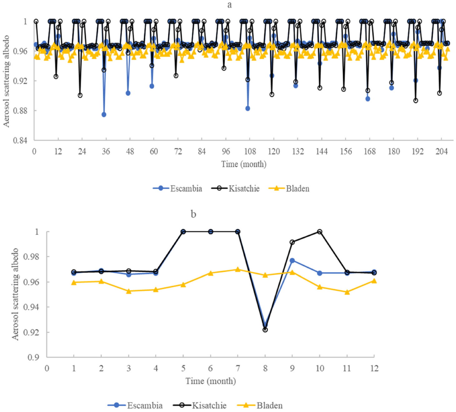
The monthly aerosol single scattering albedo at 483.5 nm was 0.97 (±0.001) in Escambia, 0.96 (±0.007) in Bladen, and 0.97 (±0.02) in Kisatchie and did not statistically differ (p > 0.05) (Figure 2a). Seasonal dynamics of aerosol single scattering albedo at 483.5 nm were similar between Escambia and Kisatchie (Figure 2b). Aerosol scattering decreased dramatically in August, however, it was relatively stable in Bladen and increased slightly during the growing season (May to September).

3.3. Black Carbon Column Mass Density

There was no significant difference in the monthly black carbon column mass density among the three areas (Figure 3a). Average black carbon column mass density was 7.46 ± 1.30 × 10⁻⁷ kg cm−2, 8.42 ± 0.81 × 10⁻⁷ kg cm−2, and 7.46 ± 1.30 × 10⁻⁷ kg cm−2 for Escambia, Bladen, and Kisatchie, respectively. Seasonal dynamics of monthly black carbon column mass density were similar among the three areas (Figure 3b). Values of black carbon column mass density increased during the springtime (March, April, and May) in the three areas and then gradually decreased.

3.4. Dust Column Mass Density

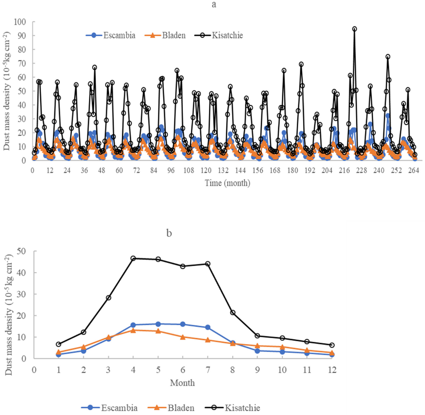
Monthly dust column mass density was significantly higher in Kisatchie (23.49 ± 1.03 × 10⁻⁵ kg cm−2) than in Escambia (7.99 ± 0.27 × 10⁻⁵ kg cm−2) or Bladen (7.41 ± 0.04 × 10⁻⁵ kg cm−2) (p < 0.05) (Figure 4a). Escambia and Bladen had no significant difference in monthly dust column mass density. Regarding seasonality, the monthly dust column mass density increased from March to July and then decreased across the three areas (Figure 4b).

3.5. Ozone Amount

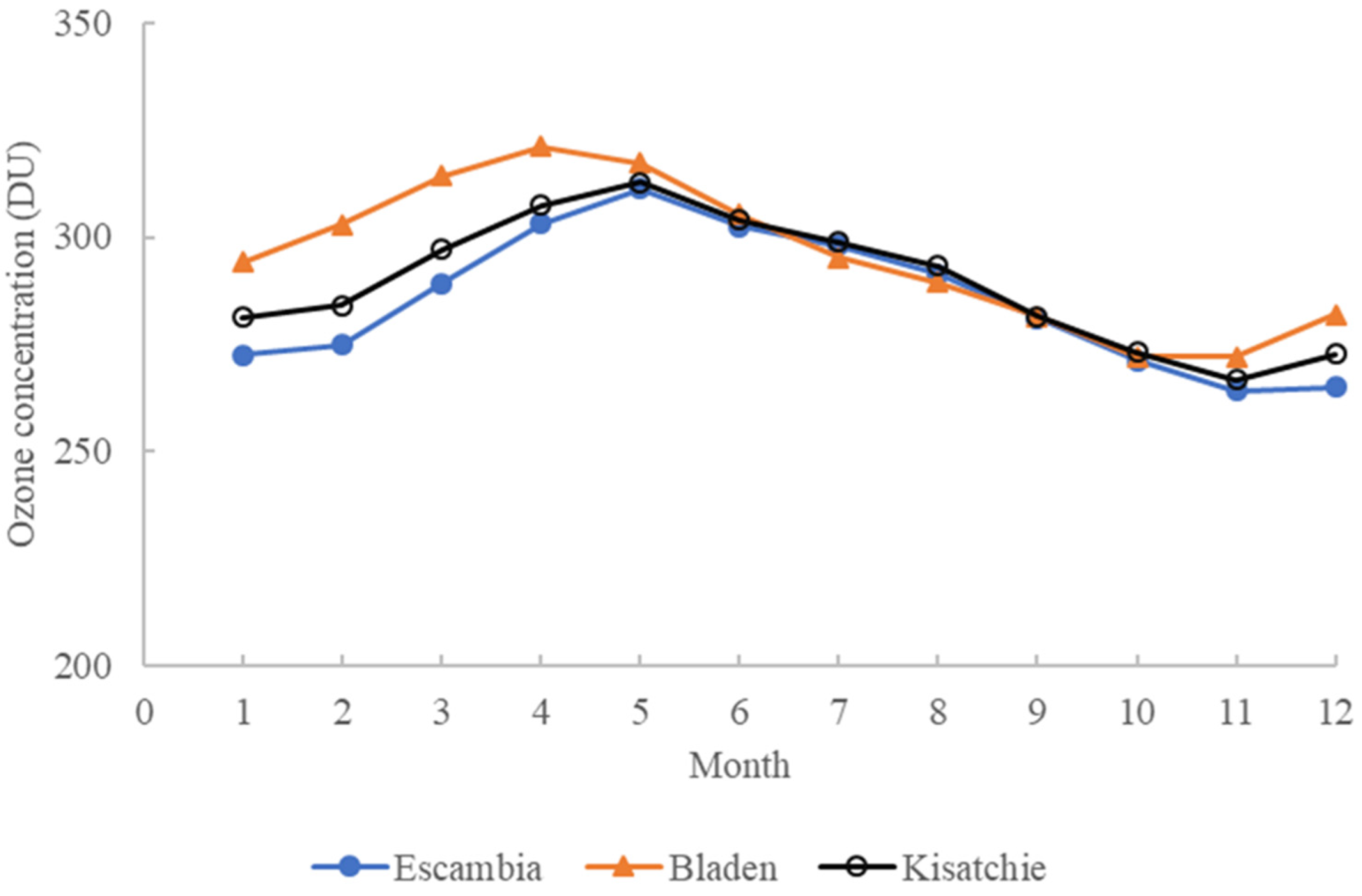
Monthly total column ozone did not statistically differ among areas (p > 0.05). Values ranged from 285.43 ± 9.57 DU in Escambia, 295.61 ± 13.72 DU in Bladen, and 289.40 ± 11.41 DU in Kisatchie. The seasonal dynamics of the monthly total column ozone were relatively stable across the three areas (Figure 5).

3.6. CO Concentration

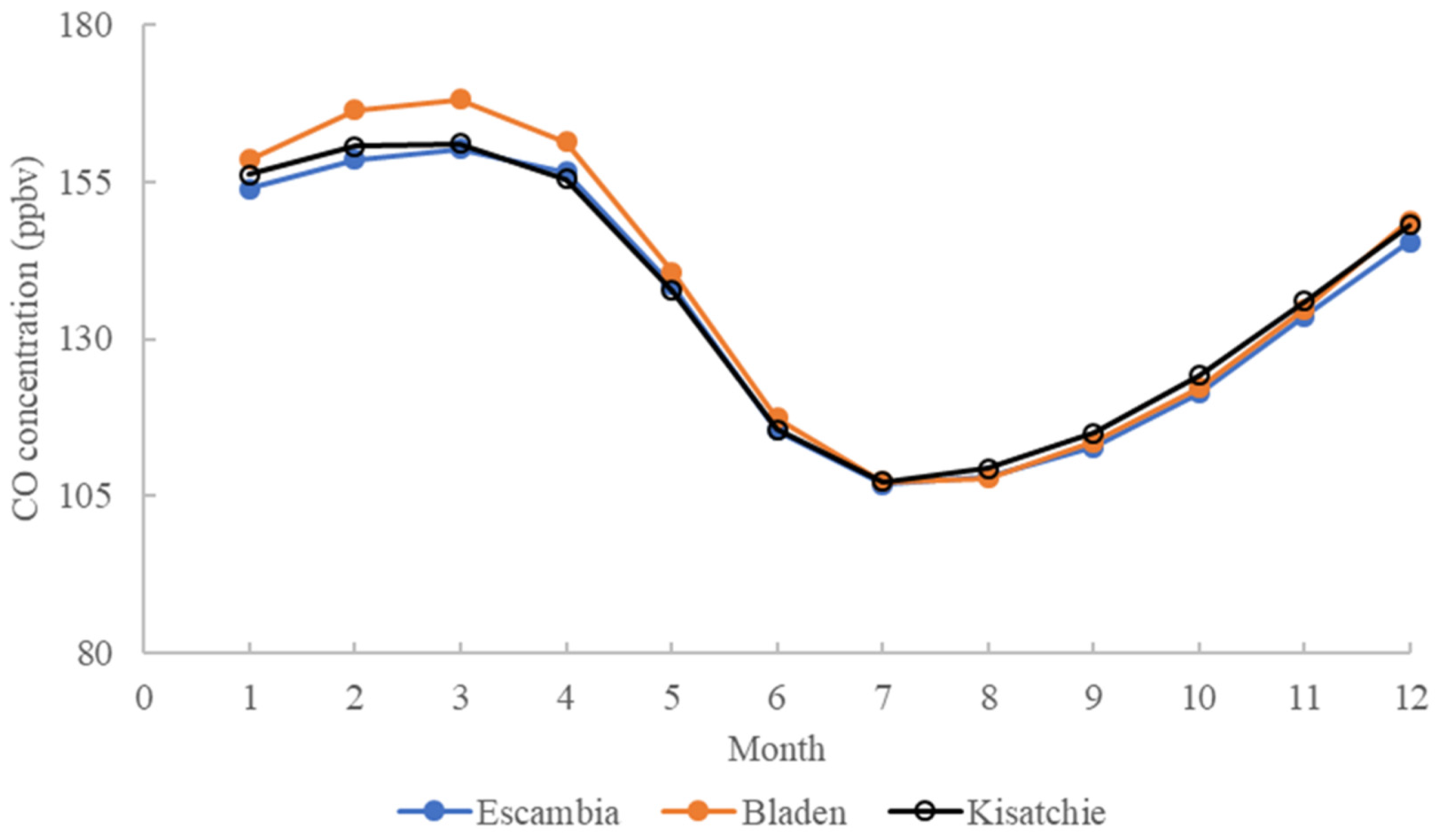
The monthly CO concentration in the air (mole fraction in the air at night time) was not statistically different among the areas. Values ranged from 134.14 ± 3.55 ppbv in Escambia, 137.02 ± 6.41 ppbv in Bladen, and 135.42 ± 2.26 ppbv in Kisatchie. CO concentration was slightly high in January, February, and March and low in June, July, and August across the three areas (Figure 6).

3.7. SO2 Density

Monthly SO2 column mass density was significantly higher in Bladen (4.42 ± 0.77 × 10⁻⁶ kg cm−2) than in Escambia (3.20 ± 1.21 × 10⁻⁶ kg cm−2) or Kisatchie (3.48 ± 1.48 × 10⁻⁶ kg cm−2) (p < 0.05) (Figure 7a). Seasonal dynamics of SO2 column mass density varied inversely in Bladen compared to Escambia and Kisatchie (Figure 7b). Seasonal SO2 column mass density varied across the areas. SO2 column mass density decreased with time until August in Bladen but increased in Escambia and Kisatchie during July, August, and September.

3.8. Albedo

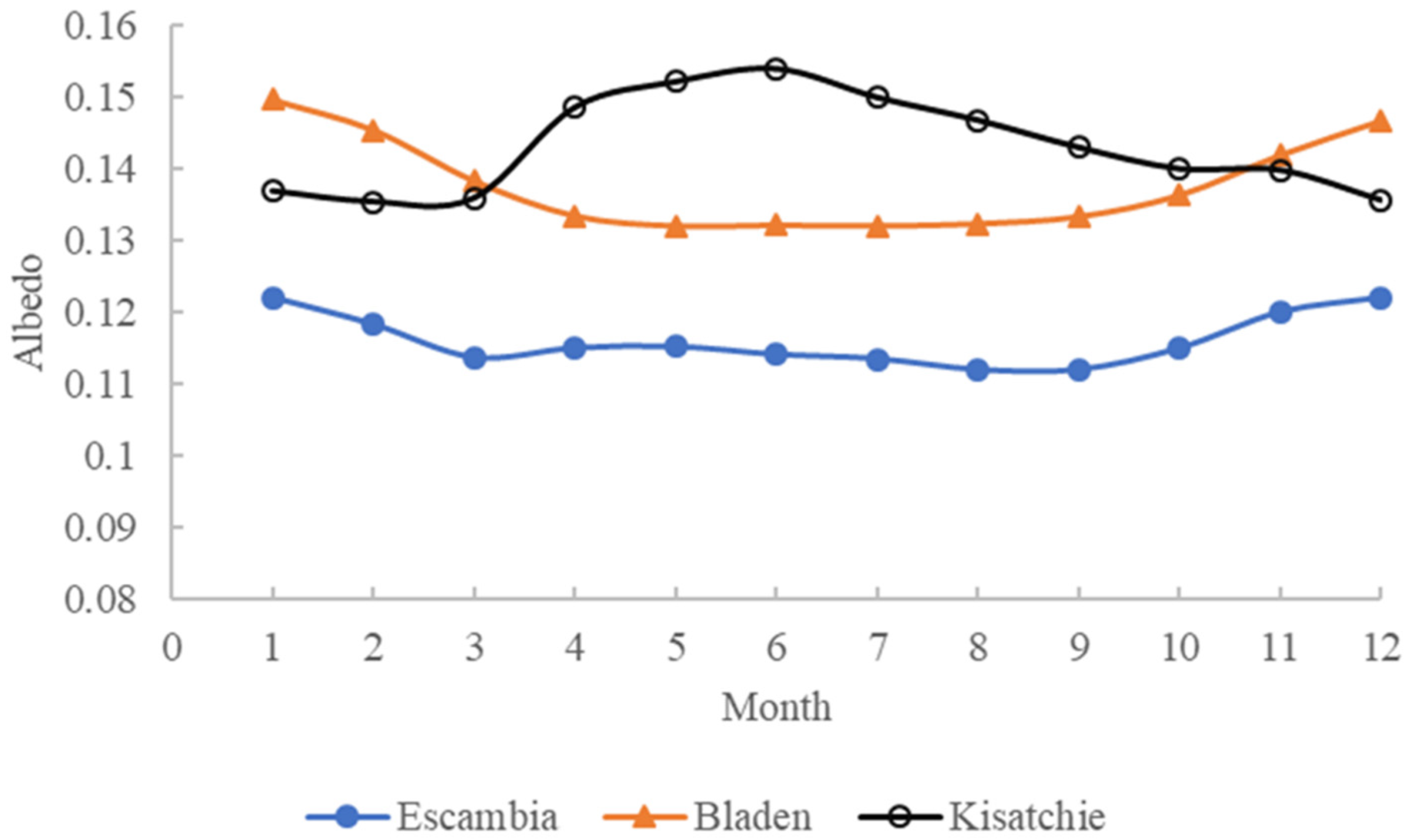
The monthly surface albedo in Escambia (0.116 ± 0.003) was significantly lower than in Bladen (0.137 ± 0.0003) or Kisatchie (0.143 ± 0.007) (p < 0.05). Seasonal dynamics of monthly surface albedo were relatively stable in Escambia and Bladen (Figure 8) but increased slightly in Kisatchie during summer.

3.9. Cloud Area Fraction

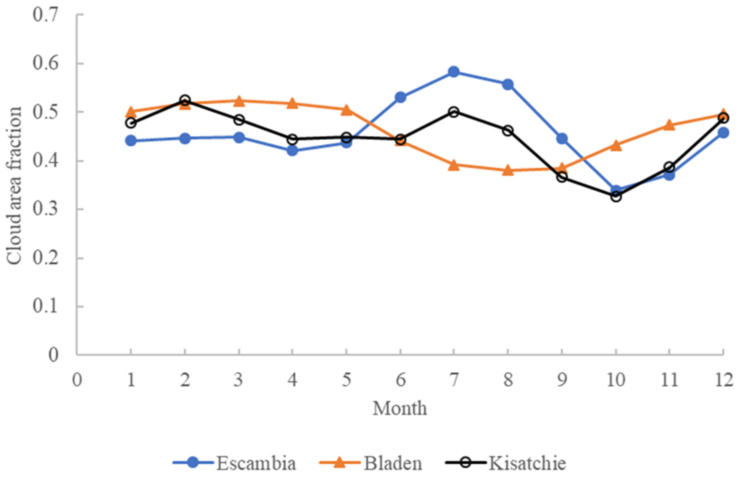
The monthly total cloud area fraction ranged from 0.456 ± 0.064 in Escambia, 0.464 ± 0.014 in Bladen, and 0.446 ± 0.049 in Kisatchie and did not statistically differ (p > 0.05). The total cloud area fraction decreased during summer and increased during fall in Bladen (Figure 9) but decreased in Escambia and Kisatchie.

3.10. Sensible Heat Net Flux

Monthly sensible heat net flux was significantly different among the three areas (p < 0.01) (Figure 10a). Bladen (46.24 ± 3.35 W m−2) had the highest net flux followed by Escambia (38.61 ± 4.94 W m−2) and Kisatchie (20.96 ± 3.86 W m−2). Seasonal dynamics of sensible heat net flux also differed across the areas (Figure 10b). Sensible heat net flux was highest during August in Bladen, while high during March-June in Escambia. In contrast, sensible heat net flux decreased slightly during April in Kisatchie.

3.11. Latent Heat Net Flux

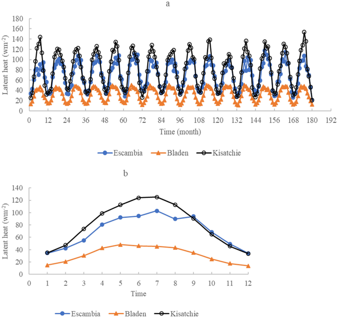
Monthly latent heat net flux was significantly different among the three areas (p < 0.01) (Figure 11a), but the pattern opposed that of sensible heat net flux (Figure 11a). Kisatchie (80.34 ± 3.33 W m−2) had the highest latent heat net flux followed by Escambia (69.88 ± 6.11 W m−2) and Bladen (31.87 ± 0.37 W m−2). Seasonal dynamics were similar across the three areas (Figure 11b) when latent heat net flux increased during the summer (e.g., April to September).

3.12. Bowen Ratio

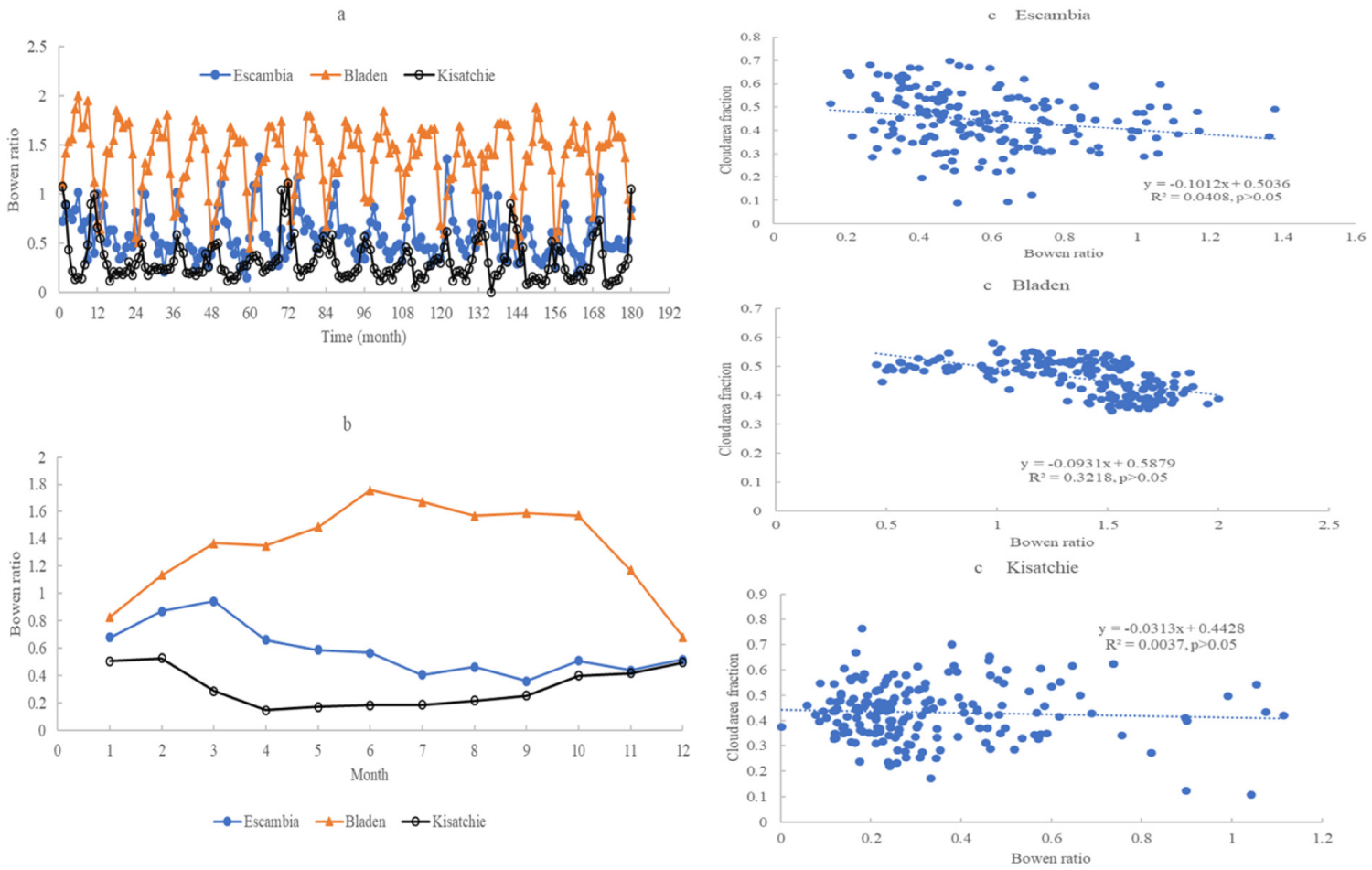
The Bowen ratio varied significantly among areas (p < 0.01) (Figure 12a). Bladen (1.35 ± 0.23) had the highest Bowen ratio, followed by Escambia (0.59 ± 0.08) and Kisatchie (0.33 ± 0.01). Bowen ratio seasonal dynamics differed among areas (Figure 12b). The Bowen ratio was high in Bladen during the growing season (April to October), while it decreased in Escambia and Kisatchie. There was no significant correlation between the monthly Bowen ratio and the total cloud area fraction in any area (Figure 12c).

3.13. Net Shortwave

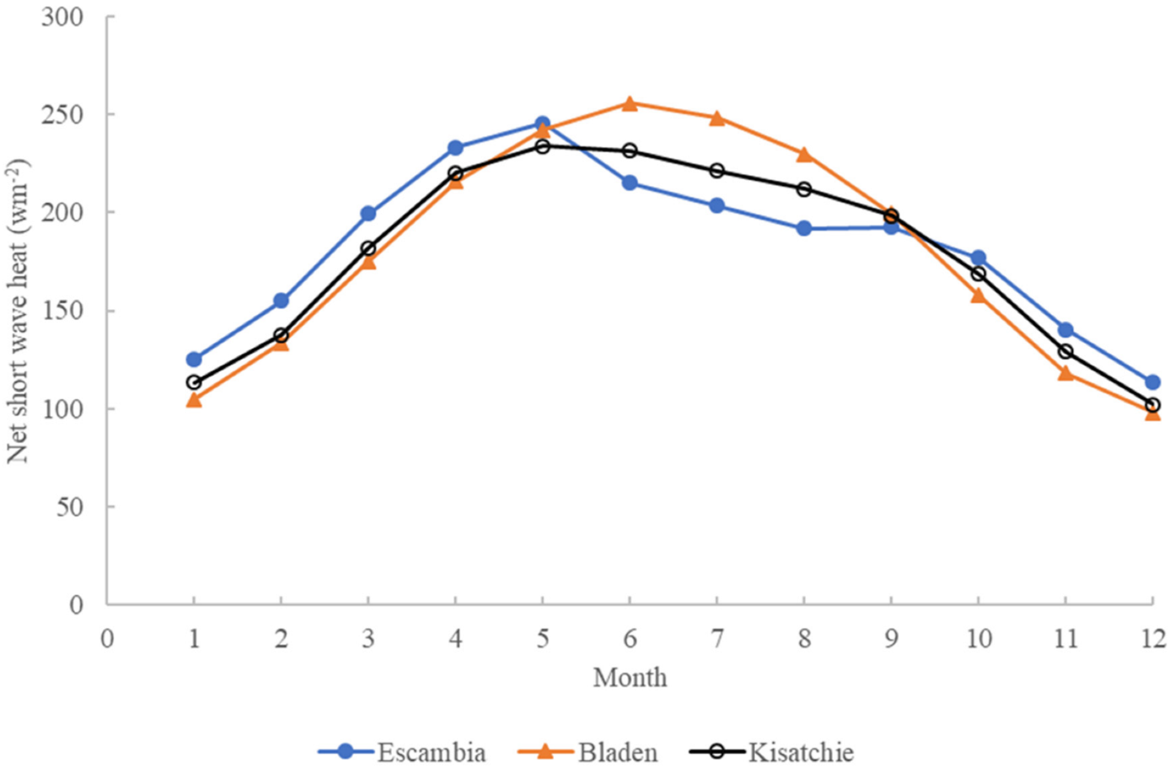
The monthly net shortwave of forest surface averaged 182.62 ± 13.05 W m−2 in Escambia, 181.43 ± 5.14 W m−2 in Bladen, and 179.13 ± 9.84 W m−2 in Kisatchie and was not statistically different among areas. Seasonal patterns of the monthly net shortwave of the forest surface were similar among areas and peaked in May or June in all areas (Figure 13).

3.14. Net Longwave

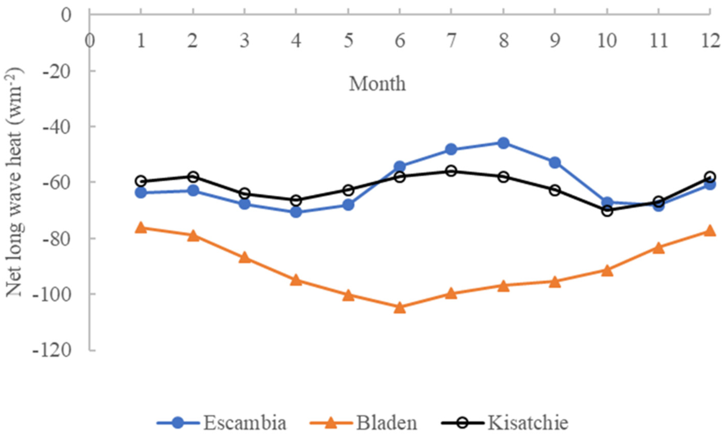
The monthly net longwave of forest surface was significantly lower in Bladen (−90.46 ± 0.65 W m−2) compared to Escambia (−60.83 ± 11.10 W m−2) and Kisatchie (−61.74 ± 6.68 W m−2) (p < 0.01). Seasonal dynamics of the net longwave of forest surface were similar between Escambia and Kisatchie but inverse in Bladen (Figure 14).

4. Discussion

Longleaf pine forests and the atmosphere can interact through particles, gases, water, and energy. The coupling in the biophysical processes contributes to the long-term variability of atmospheric processes [32]. Interactions between forests and the atmosphere are considered to be responsible for regional climate disasters (e.g., extreme drought) [33]. Therefore, understanding the interactions between forests and the atmosphere may help identify the mechanisms of the existence (or resilience) of the longleaf pine forest ecosystem under climate change in the southeastern region [34]. Remote sensing data (e.g., MODIS) from different satellites could be used as benchmarks to monitor these biophysical processes from different perspectives at a regional level.

4.1. Aerosol Optical Depth

There are different wavelengths to measure AOD, such as 342.5 nm, 442 nm, and others. In this study, we only selected the wavelength of 483.5 nm because the measurements from other wavelengths are either too small or contained invalid data. However, the wavelength of 483.5 nm provided suitable AOD measurements for the three areas.
The composition of atmospheric aerosols is complex and may include various trace metals, inorganic oxides, sulfates, nitrates, fire plumes, and organic compounds from plants [35]. AOD has been broadly used as an essential index of air quality in the atmosphere [36]. The smaller the AOD, the cleaner the atmosphere, and vice versa. The effects of aerosol on plants can (i) direct influence plant stomatal conductance, respiration, and photosynthesis, and (ii) indirectly affect rainfall and scatter sunlight [37]. In this study, the average monthly AOD at 483.5 nm in the three areas over the past 22 years was around 0.02, and the aerosol single scattering albedo was about 0.97. With the exception of August, Kisatchie had a low AOD. This result corresponds with the decreased aerosol single scattering albedo in Kisatchie during August. This pattern frequently occurred and might be related to local human activities, such as agricultural practices (e.g., rice harvesting and burning). Furthermore, this result is consistent with trends in monthly dust column mass density, which was significantly higher in Kisatchie than in Escambia or Bladen. The possible causes for this pattern may be also related to agricultural practices as Louisiana is a major producer of sugarcane, soybeans, corn, cotton, and rice. Crop harvesting and burning residual biomass in a large area can increase atmospheric dust. Additionally, this study area is close to the urban areas (Alexandria and Pineville, LA, USA). The pollutants and dust from urban and agricultural areas could be dispersed to the surrounding forest area.

4.2. Black Carbon

The monthly black carbon column mass density was similar among areas. The measurement was high during the springtime (February to May). This result is consistent with the prescribed burning, which is broadly used to control broadleaved tree species in longleaf pine forests [38]. Black carbon in the atmosphere can affect human health and climate [39,40]. Increases in black carbon have been linked with health problems, including respiratory and cardiovascular disease and congenital disabilities. Moreover, black carbon can absorb light as heat, warm the air, and rapidly change rain and cloud patterns. Further research should be conducted to explore the relationship between prescribed burning, black carbon production, and health and environmental effects.

4.3. Trace Gases

Forests can also influence the emissions of trace gases. In this study, both ozone and CO are relatively stable. The monthly total column ozone is about 290 DU across the three areas, and the monthly CO concentration is about 135 ppbv. However, the monthly SO2 column mass density was significantly higher in Bladen than in Escambia and Kisatchie. The seasonal dynamics of SO2 column mass density in Bladen were the opposite of that observed in Escambia and Kisatchie. Since atmospheric SO2 is mainly derived from fossil burning, this might be related to the local industrial facilities due to the high local population.

4.4. Albedo

Surface albedo, which changes solar radiation and energy allocation, can be modified by changes in forest cover and tree species composition [30]. In this study, the monthly surface albedo in Escambia was significantly lower than that in Bladen and Kisatchie. Additionally, seasonal albedo dynamics were relatively stable in Escambia and Bladen, while albedo increased slightly in Kisatchie during the summer months. This pattern may be related to the broadleaved trees in each area. Deciduous trees could increase surface albedo due to the growth of leaves during summertime. Thus, restoration prescriptions that remove hardwood species from longleaf pine forests at a large scale may decrease the surface albedo and potentially increase local air temperature.

4.5. Heat Net Flux

Remote sensing data can be used to study the water and energy exchanges above the forest canopy-atmosphere interface [41,42]. Our results indicate that the monthly heat net flux (sensible and latent) was significantly different among the three areas, which led to different Bowen ratios. Variations in the Bowen ratio may be an indicator of longleaf pine resilience to environmental stress. For example, the Bowen ratio doubled under drought conditions [24]. The biophysical effects (e.g., albedo) of forest cover not only influence air temperature above the forest canopies, but also the understory energy budget through shading, air mixing, and evapotranspiration processes which ultimately influences the air and soil temperature conditions at ground level [43]. Our results suggest that the Bowen ratio and total cloud area fraction are not significantly correlated. This point differs from the findings of previous reports [44]. One possible reason for this discrepancy might be the complicated landscape, such as pine forests of different ages (e.g., young and mature) or structures in these areas. Additionally, all kinds of clouds (convection and cumuli) were included each month during the growing and nongrowing seasons. Cloud formation in a large area is not only related to water vapor but also to aerosols, wind, and other factors.

4.6. Net Shortwave and Longwave Heat

The monthly net shortwave of the forest surface and its seasonal dynamics were not significantly different among the three areas. However, the net longwave of the forest surface was lower (high negative) in Bladen than in Escambia and Kisatchie, meaning that longleaf pine forests emitted more longwave energy to the atmosphere and surroundings. This point may be related to solar radiation utilization, disturbances, and forest canopy structure under biological processes [45,46]. The previously mentioned high sensible heat and Bowen ratio may be related to this high longwave emission. Since our study covers a large geographical area, more detailed data should be collected to explain the differences in the three areas. However, the differences in energic processes may provide implications to include an energetic perspective while managing longleaf pine forests on a large scale with multiple objectives (e.g., timber, biodiversity, environment, and climate) [47].

5. Conclusions

Longleaf pine forests require frequent burning to prevent their successional replacement on most sites. While the re-establishment of a frequent burning regime will help sustain critical flora and fauna, it is uncertain what impacts frequent fire will have on atmospheric conditions. One critical step in answering this question is to study its current interactions with the atmosphere on a large scale. Multiple satellite data from NASA EarthData have provided continuous and quantitative measurements on the earth’s surface (above forest canopies) at different spatial and temporal scales, which cannot be achieved from other methods. We explored remote sensing data over the past 22 years to document and compare the complex interactions of particles, gasses, and energy with the atmosphere in three areas with active longleaf pine restoration programs. This study indicates there are spatial and temporal homogeneities (e.g., AOD and black carbon) and heterogeneities (e.g., albedo and Bowen ratio) in these interactions. Studying these biophysical interactions will be helpful for the large-scale longleaf pine forest restoration and management under climate change with multiple objectives (e.g., timber, biodiversity, air quality, climate, and public health). Our findings provide insight into how forest restoration practices influence air quality and greenhouse gas emissions. Further research to integrate the necessary ground information is needed to clarify underlying mechanisms.

Author Contributions

X.C. and J.L.W.: conceptualization; data analysis; investigation; methodology; visualization; writing; reviewing. All authors have read and agreed to the published version of the manuscript.

Funding

This research was supported by the USDA National Institute of Food and Agriculture Capacity Building Program (2021-38821-34596), the McIntire Stennis project, AAMU-RISE with Raytheon, and the USDA Forest Service.

Data Availability Statement

The data presented in this study are available at NASA Earthdata.

Acknowledgments

This paper was written and prepared in part by a U.S. Government employee on official time, and therefore it is in the public domain and not subject to copyright. The findings and conclusions in this publication are those of the author(s) and should not be construed to represent an official USDA, Forest Service, or United States Government determination or policy.

Conflicts of Interest

The authors declare that there is no conflict of interest.

References

  1. Hodges, A.W. The naval stores industry. In The Longleaf Pine Ecosystem: Ecology, Silviculture, and Restoration; Jose, S., Jokela, E.J., Miller, D.L., Eds.; Springer: Berlin/Heidelberg, Germany, 2006; pp. 43–48. [Google Scholar]
  2. Jose, S.; Jokela, E.J.; Miller, D.L. The Longleaf Pine Ecosystem: An overview. In The Longleaf Pine Ecosystem: Ecology, Silviculture, and Restoration; Jose, S., Jokela, E.J., Miller, D.L., Eds.; Springer: Berlin/Heidelberg, Germany, 2006; pp. 3–8. [Google Scholar]
  3. Frost, C.C. History and future of the longleaf pine ecosystem. In The Longleaf Pine Ecosystem: Ecology, Silviculture, and Restoration; Jose, S., Jokela, E.J., Miller, D.L., Eds.; Springer: Berlin/Heidelberg, Germany, 2006; pp. 9–42. [Google Scholar]
  4. Carter, M.C.; Kellison, R.C.; Wallinger, R.S. Forestry in the US South: A history; Louisiana State University Press: Baton Rouge, LA, USA, 2015. [Google Scholar]
  5. Matthews, J.M.; Hinchee, J.; Guldin, J.M. Restoration of Longleaf Pine in the Southern Region of the US Forest Service: An Overview of the Million-Acre Challenge; e–Gen. Tech. Rep. SRS–253; US Department of Agriculture, Forest Service, Southern Research Station: Asheville, NC, USA, 2020; Volume 253, pp. 112–119.
  6. Horton, A.J.; Lehtinen, J.; Kummu, M. Targeted land management strategies could halve peatland fire occurrences in Central Kalimantan, Indonesia. Commun. Earth Environ. 2022, 3, 204. [Google Scholar] [CrossRef]
  7. Platt, W.J.; Carr, S.M.; Reilly, M.; Fahr, J. Pine savanna overstorey influences on ground-cover biodiversity. Appl. Veg. Sci. 2016, 9, 37–50. [Google Scholar] [CrossRef]
  8. Rother, M.T.; Huffman, J.M.; Guiterman, C.H.; Robertson, K.M.; Jones, N. A history of recurrent, low-severity fire without fire exclusion in southeastern pine savannas, USA. For. Ecol. Manag. 2020, 475, 118406. [Google Scholar] [CrossRef]
  9. Natural Resource Conservation Service (NRCS); USDA. Longleaf Pine Ecosystem Restoration. FY20-24 Implementation Strategy; USDA: Washington, DC, USA, 2020.
  10. Platt, W.J.; Evans, G.W.; Rathbun, S.L. The population dynamics of a long-lived conifer (Pinus palustris). Am. Nat. 1988, 131, 491–525. [Google Scholar] [CrossRef]
  11. Samuelson, L.J.; Stokes, T.A.; Butnor, J.R.; Johnsen, K.H.; Gonzalez-Benecke, C.A.; Martin, T.A.; Cropper, W.P., Jr.; Anderson, P.H.; Ramirez, M.R.; Lewis, J.C. Ecosystem carbon density and allocation across a chronosequence of longleaf pine forests. Ecol. Appl. 2017, 27, 244–259. [Google Scholar] [CrossRef]
  12. Guldin, J.M. Restoration of native fire-adapted southern pine-dominated forest ecosystems: Diversifying the tools in the silvicultural toolbox. For. Sci. 2019, 65, 508–518. [Google Scholar] [CrossRef] [Green Version]
  13. Johnson, R.; Gjerstad, D. Restoring the overstory of longleaf pine ecosystems. In The Longleaf Pine Ecosystem: Ecology, Silviculture, and Restoration; Jose, S., Jokela, E.J., Miller, D.L., Eds.; Springer: Berlin/Heidelberg, Germany, 2006; pp. 271–295. [Google Scholar]
  14. Hu, H.; Wang, G.G.; Walke, J.L.; Knapp, B.O. Silvicultural treatments for converting loblolly pine to longleaf pine dominance: Effects on planted longleaf pine seedlings. For. Ecol. Manag. 2012, 276, 209–216. [Google Scholar] [CrossRef]
  15. Upchurch, G.E., Jr.; Otto-Bliesner, B.L.; Scotese, C. Vegetation-atmosphere interactions and their role in global warming during the latest Cretaceous. Philos. Trans. R. Soc. London. Ser. B 1998, 353, 97–112. [Google Scholar] [CrossRef] [Green Version]
  16. Baldocchi, D.D.; Hincks, B.B.; Meyers, T.P. Measuring biosphere-atmosphere exchanges of biologically related gases with micrometeorological methods. Ecology 1988, 69, 1331–1340. [Google Scholar] [CrossRef]
  17. Liu, Y.-Q.; Goodrick, S.; Heilman, W. Wildland fire emissions, carbon, and climate: Wildfire-climate interactions. For. Ecol. Manag. 2014, 317, 80–96. [Google Scholar] [CrossRef]
  18. Heilman, W.E.; Liu, Y.; Urbanski, S.; Kovalev, V.; Mickler, R. Wildland fire emissions, carbon, and climate: Plume rise, atmospheric transport, and chemistry processes. For. Ecol. Manag. 2014, 317, 70–79. [Google Scholar] [CrossRef]
  19. United Nations Economic and Social Council, Working Group on Strategies and Review. Prioritizing Reductions of Particulate Matter from Sources that are also Significant Sources of Black Carbon-Analysis and Guidance. In Proceedings of the Fifty-Ninth Session, Geneva, Switzerland, 18–21 May 2021; Available online: https://unece.org/sites/default/files/2021-04/ECE_EB.AIR_WG.5_2021_8-2102625E.pdf (accessed on 20 October 2022).
  20. Ainsworth, E.A.; Long, S.P. What have we learned from 15 years of free-air CO2 enrichment (FACE)? A meta-analytic review of the responses of photosynthesis, canopy properties and plant production to rising CO2. New Phytol. 2005, 165, 351–372. [Google Scholar] [CrossRef] [PubMed]
  21. Zak, D.R.; Kubiske, M.E.; Pregitzer, K.S.; Burton, A.J. Atmospheric CO2 and O3 alter competition for soil nitrogen in developing forests. Glob. Chang. Biol. 2012, 18, 1480–1488. [Google Scholar] [CrossRef]
  22. Friedel, M.; Chiodo, G.; Stenke, A.; Domeisen, D.I.V.; Fueglistaler, S.; Anet, J.G.; Peter, T. Springtime arctic ozone depletion forces northern hemisphere climate anomalies. Nat. Geosci. 2022, 15, 541–547. [Google Scholar] [CrossRef]
  23. Goldstein, A.H. Biosphere and Atmosphere Interactions in Sierra Nevada Forests. In Proceedings of the Sierra Nevada Science Symposium, Kings Beach, CA, USA, 7–10 October 2002. [Google Scholar]
  24. Whelan, A.; Starr, G.; Staudhammer, C.L.; Loescher, H.W.; Mitchell, R.J. Effects of drought and prescribed fire on energy exchange in longleaf pine ecosystems. Ecosphere 2015, 6, 128. [Google Scholar] [CrossRef]
  25. Salomonson, V.V.; Barnes, W.L.; Maymon, W.P.; Montgomery, H.; Ostrow, H. MODIS: Advanced facility instrument for studies of the Earth as a system. IEEE Trans. Geosci. Remote Sens. 1989, 27, 145–153. [Google Scholar] [CrossRef]
  26. Velpuri, N.M.; Senay, G.B.; Singh, R.K.; Bohms, S.; Verdin, J.P. A comprehensive evaluation of two MODIS evapotranspiration products over the conterminous United States: Using point and gridded FLUXNET and water balance ET. Remote Sens. Environ. 2013, 139, 35–49. [Google Scholar] [CrossRef]
  27. Famiglietti, C.A.; Fisher, J.B.; Halverson, G.; Borbas, E.E. Global validation of MODIS near-surface air and dew point temperatures. Geophys. Res. Lett. 2018, 45, 7772–7780. [Google Scholar] [CrossRef] [Green Version]
  28. Luo, L.; Robock, A.; Mitchell, K.E.; Houser, P.R.; Wood, E.F.; Schaake, J.C.; Lohmann, D.; Cosgrove, B.; Wen, F.; Sheffield, J.; et al. Validation of the North American Land Data Assimilation System (NLDAS) retrospective forcing over the southern Great Plains. J. Geophys. Res. 2003, 108, 8843. [Google Scholar] [CrossRef]
  29. Mitchell, K.E.; Lohmann, D.; Houser, P.R.; Wood, E.F.; Schaake, J.C.; Robock, A.; Cosgrove, B.A.; Sheffield, J.; Duan, Q.; Luo, L.; et al. The multi-institution North American Land Data Assimilation System (NLDAS): Utilizing multiple GCIP products and partners in a continental distributed hydrological modeling system. J. Geophys. Res. 2004, 109, D07S90. [Google Scholar] [CrossRef]
  30. Chen, X. A case study of using remote sensing data to compare biophysical properties of a forest and an urban area in northern Alabama, USA. J. Sustain. For. 2016, 35, 261–279. [Google Scholar] [CrossRef]
  31. Chen, X.; Chen, H. Comparing environmental impacts of Chinese Torreya plantations and regular forests using remote sensing. Environ. Dev. Sustain. 2021, 23, 133–150. [Google Scholar] [CrossRef]
  32. Liu, Y.-Q. Monthly and seasonal variability of the land-atmosphere system. World Sci. Ser. Meteorol. East Asia 2004, 3, 73–91. [Google Scholar]
  33. Xue, Y.; Shukla, J. The influence of land surface properties on Sahel climate. Part 1: Desertification. J. Clim. 1993, 6, 2232–2245. [Google Scholar] [CrossRef]
  34. Chen, X.; Guo, Q.; Bowman, K.A. Climate variation within the range of longleaf pine forests during the past century. Atmosphere 2022, 13, 465. [Google Scholar] [CrossRef]
  35. Dubovik, O.; Holben, B.; Eck, T.F.; Smirov, A.; Kaufman, Y.J.; King, M.D.; Tanre, D.; Slutsker, I. Variability of absorption and optical properties of key aerosol types observed in worldwide locations. J. Atmos. Sci. 2002, 59, 590–608. [Google Scholar] [CrossRef]
  36. Eck, T.F.; Holben, B.N.; Reid, J.S.; Dubovik, O.; Smirnov, A.; O’Neill, N.T.; Slutsker, I.; Kinne, S. Wavelength dependence of the optical depth of biomass burning, urban, and desert dust aerosols. J. Geophys. Res. Atmos. 1999, 104, 31333–31349. [Google Scholar] [CrossRef]
  37. Cohan, D.S.; Xu, J.; Greenwald, R.; Bergin, M.H.; Chameides, W.L. Impact of atmospheric aerosol light scattering and absorption on terrestrial net primary productivity. Glob. Biogeochem. Cycles 2002, 16, 37-1–37-12. [Google Scholar] [CrossRef]
  38. Boyer, W.D. Growing-Season Burns for Control of Hardwoods in Longleaf Pine Stands; US Department of Agriculture, Forest Service, Southern Forest Experiment Station: New Orleans, LA, USA, 1990.
  39. Bond, T.C.; Doherty, S.J.; Fahey, D.W.; Forster, P.M.; Berntsen, T.; DeAngelo, B.J.; Flanner, M.G.; Ghan, S.; Kärcher, B.; Koch, D.; et al. Bounding the role of black carbon in the climate system: A scientific assessment. J. Geophys. Res. Atmos. 2013, 118, 5380–5552. [Google Scholar] [CrossRef]
  40. Anenberg, S.C.; Schwartz, J.; Shindell, D.; Amann, M.; Faluvegi, G.; Klimont, Z.; Janssens-Maenhout, G.; Pozzoli, L.; Van Dingenen, R.; Vignati, E.; et al. Global air quality and health co-benefits of mitigating near-term climate change through methane and black carbon emission controls. Environ. Health Perspect. 2012, 120, 831–839. [Google Scholar] [CrossRef] [Green Version]
  41. Baldocchi, D.; Falge, E.; Gu, L.; Olson, R.; Hollinger, D.; Running, S.; Wofsy, S. FLUXNET: A new tool to study the temporal and spatial variability of ecosystem-scale carbon dioxide, water vapor, and energy flux densities. Bull. Am. Meteorol. Soc. 2001, 82, 2415–2434. [Google Scholar] [CrossRef]
  42. Li, Y.; Zhao, M.; Motesharrei, S.; Mu, Q.; Kalnay, E.; Li, S. Local cooling and warming effects of forests based on satellite observations. Nat. Commun. 2015, 6, 6603. [Google Scholar] [CrossRef] [PubMed] [Green Version]
  43. Zellweger, F.; Coomes, D.; Lenoir, J.; Depauw, L.; Maes, S.L.; Wulf, M.; De Frenne, P. Seasonal drivers of understorey temperature buffering in temperate deciduous forests across Europe. Glob. Ecol. Biogeogr. 2019, 28, 1774–1786. [Google Scholar] [CrossRef] [PubMed] [Green Version]
  44. Manoli, G.; Demec, J.-C.; Novick, K.; Oishi, A.C.; Noormets, A.; Marani, M.; Katual, G. Soil–plant–atmosphere conditions regulating convective cloud formation above southeastern US pine plantations. Glob. Chang. Biol. 2016, 22, 2238–2254. [Google Scholar] [CrossRef] [PubMed]
  45. Müller, F.; Kroll, F. Integrating ecosystem theories-Gradients and orientors as outcomes of self-organized processes. Int. J. Des. Nat. Ecodynamics 2011, 6, 318–341. [Google Scholar] [CrossRef]
  46. Marín, D.; Martín, M.; Serrot, P.H.; Sabater, B. Thermodynamic balance of photosynthesis and transpiration at increasing CO2 concentrations and rapid light fluctuations. BioSystems 2014, 116, 21–26. [Google Scholar] [CrossRef] [PubMed]
  47. Chen, X. Energetics of forest biomes. Funct. Commun. Ecosys. 2007, 1, 49–55. [Google Scholar]
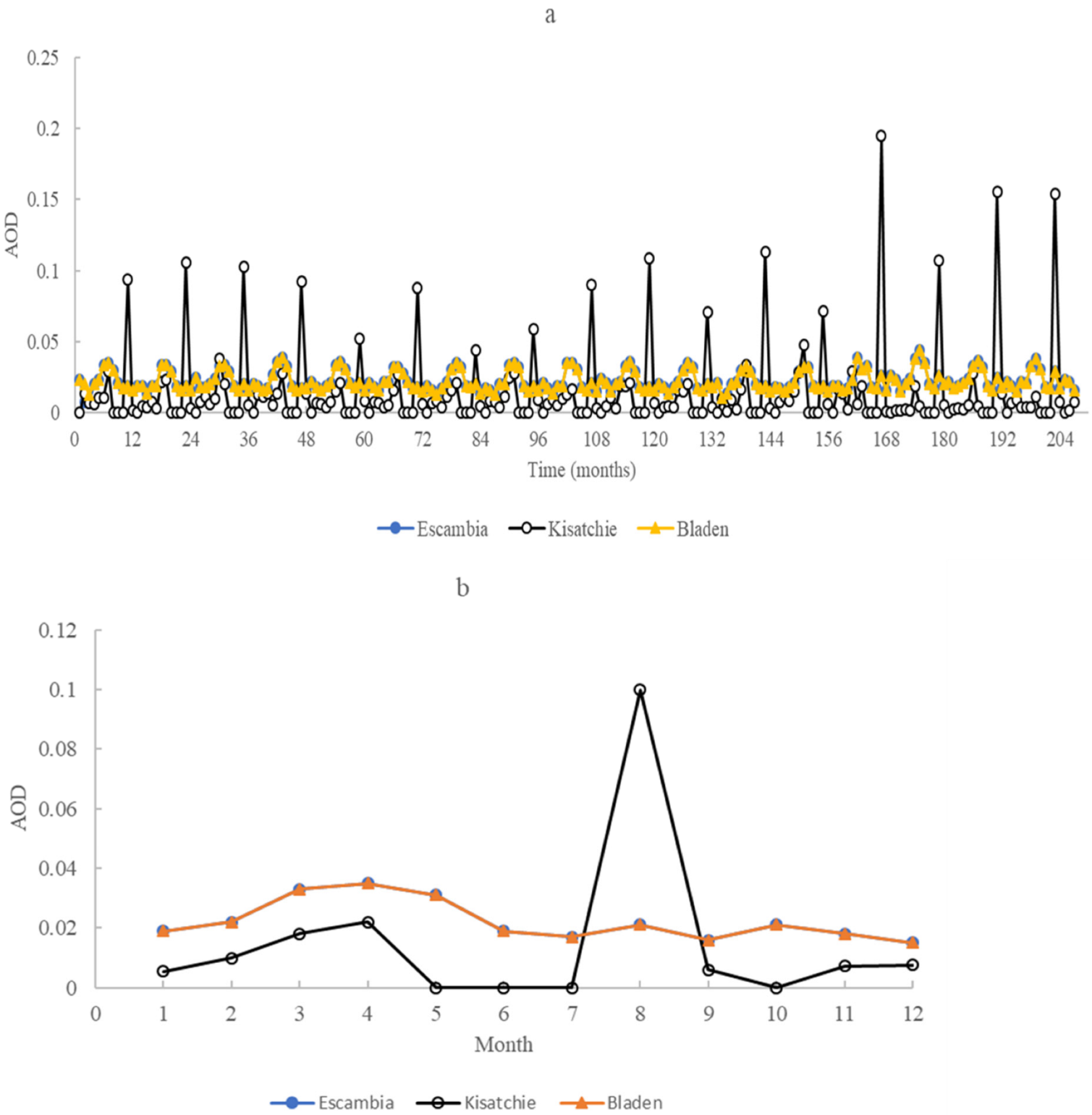
Figure 1. Dynamics of aerosol optical depth (AOD) at 483.5 nm in Escambia, Bladen, and Kisatchie (a) Monthly and yearly dynamics of AOD from October 2004; (b) The integrated monthly average of AOD.
Atmosphere 13 01733 g001
Figure 2. Dynamics of aerosol single scattering albedo at 483.5 nm in Escambia, Bladen, and Kisatchie. (a) Monthly and yearly dynamics of aerosol single scattering from October 2004; (b) The integrated monthly average of aerosol single scattering.
Atmosphere 13 01733 g002
Figure 3. Dynamics of black carbon column mass density in Escambia, Bladen, and Kisatchie. (a) Monthly and yearly dynamics of black carbon column mass density in the three areas from January 2000. (b) The integrated monthly average of black carbon column mass density.
Atmosphere 13 01733 g003
Figure 4. Dynamics of dust column mass density in Escambia, Bladen, and Kisatchie. (a) Monthly and yearly dynamics of dust column mass density from January 2000. (b) The integrated monthly average of dust column mass density.
Atmosphere 13 01733 g004
Figure 5. The integrated monthly average of total column ozone in the three areas.
Atmosphere 13 01733 g005
Figure 6. The integrated monthly CO concentration in air at night time in the three areas.
Atmosphere 13 01733 g006
Figure 7. Dynamics of SO2 column mass density in Escambia, Bladen, and Kisatchie. (a) Monthly and yearly SO2 column mass density from January 2000. (b) The integrated monthly average SO2 column mass density.
Atmosphere 13 01733 g007
Figure 8. The integrated monthly average of albedo in Escambia, Bladen, and Kisatchie.
Atmosphere 13 01733 g008
Figure 9. The integrated monthly total cloud area fraction in Escambia, Bladen, and Kisatchie.
Atmosphere 13 01733 g009
Figure 10. Dynamics of sensible heat net flux in Escambia, Bladen, and Kisatchie. (a) The monthly and yearly sensible heat net flux from January 2000. (b) The integrated monthly average of sensible heat net flux.
Atmosphere 13 01733 g010
Figure 11. Dynamics of latent heat net flux in Escambia, Bladen, and Kisatchie. (a) Monthly and yearly latent heat net flux from January 2000. (b) The integrated monthly average of latent heat net flux.
Atmosphere 13 01733 g011
Figure 12. Dynamics of Bowen ratio in the three areas. (a) Monthly and yearly Bowen ratio in the three areas from January 2000. (b) The integrated monthly average of Bowen ratio. (c) The relationship between Bowen ratio and total cloud area fraction in the three areas.
Atmosphere 13 01733 g012
Figure 13. Dynamics of the integrated monthly net shortwave in the three areas.
Atmosphere 13 01733 g013
Figure 14. Dynamics of the integrated monthly net longwave in the three areas.
Atmosphere 13 01733 g014
Table 1. The basic information of three areas with active restoration of longleaf pine forests.
AreasLatitude (N) and Longitude (E)Annual PrecipitationMean Annual Air TemperatureAverage ElevationSoil TypeProximity to Urban Area
EscambiaN 30.5°–31°
E 86.4°–87.1°
156 cm18 °C27 mUltisolsNo
BladenN 34.5°–35°
E 78°–78.7°
120 cm17 °C20 mUltisolsSmall towns
KisatchieN 31.5°–32°
E 91.5°–92.2°
146 cm16 °C80 mUltisols,
Entisols
Alexandria
Table 2. The measurement information from satellites and the derived.
IndicesUnitTimeScale
Aerosol optical depthunitlessOctober 2004–December 2021Daily, 0.25°
Single scattering albedom m−1October 2004–December 2021Daily, 0.25°
Black carbon column mass densitykg cm−2January 2000–December 2021Monthly, 0.5° × 0.625°
Dust column mass densitykg cm−2January 2000–December 2021Monthly, 0.5° × 0.625°
Total column ozoneDUOctober 2004–December 2021Daily, 0.25°
CO mole fraction in the airppbvSeptember 2002–September 2016Daily, 1°
SO2 column mass densitykg cm−2January 2000–December 2021Monthly, 0.5° × 0.625°
AlbedoW W−1January 2000–December 2021Daily, 0.25°
Total cloud area fractionm2 m−2January 2000–December 2021Monthly, 0.5° × 0.625°
Sensible heat net fluxW m−2January 2000–December 2014Monthly, 0.25°
Latent heat net fluxW m−2January 2000–December 2014Monthly, 0.25°
Bowen ratioW W−1January 2000–December 2014Monthly, 0.25°
Net shortwave of surfaceW m−2January 2000–December 2021Monthly, 0.25°
Net longwave of surfaceW m−2January 2000–December 2021Monthly, 0.25°
Publisher’s Note: MDPI stays neutral with regard to jurisdictional claims in published maps and institutional affiliations.