Abstract
In order to focus on pentad-scale precipitation forecasts, we investigated the coupling relationship between 500 hPa geopotential height (Z500) anomalies and precipitation anomalies using the China Meteorological Administration Global Land Surface ReAnalysis Interim (CRA40/Land) gridded precipitation dataset from 1999 to 2018 and the National Centers for Environmental Prediction 1 reanalysis dataset for Z500. We obtained a dynamical–statistical downscaling model (DSDM) on the pentad scale and used the daily Z500 forecast product for sub-seasonal to seasonal forecasts (15–60 days) of the FGOALS-f2 model as the predictor. Our results showed that pentad-scale prediction of precipitation is the key to bridging the current deficiencies in sub-seasonal forecasts. Compared with the FGOALS-f2 model, the pentad DSDM had a higher skill for prediction of precipitation in China at lead times longer than four pentads throughout the year and of two pentads in the summer months. FGOALS-f2 had excellent precipitation predictability at lead times less than three pentads (15 days), so the proposed pentad DSDM could not perform better than FGOALS-f2 in this period. However, at lead times greater than four pentads, the precipitation prediction scores (such as the anomaly correlation coefficient (ACC), the temporal correlation coefficient (TCC) and the mean square skill score (MSSS)) of the pentad DSDM for the whole of China were higher than those of the FGOALS-f2 model. With the rate of increase ranging from 76% to 520%, the mean ACC scores of pentad DSDM were basically greater than 0.04 after a lead time of five pentads, whereas those of the FGOALS-f2 were less than 0.04. An analysis of the Zhengzhou “720” super heavy rainstorm event showed that the pentad DSDM also had better predictability for the distribution of precipitation at lead times of three pentads than the FGOALS-f2 model for the extreme precipitation event.
1. Introduction
Extended range predictability (with forecast times of 10–30 days) is limited in dynamic forecast models as a result of the chaotic nature of the Earth’s atmosphere and the computational errors in numerical simulations [1]. For model forecasts with lead times longer than four weeks, the predictability contribution of the boundary conditions is larger than that of the initial conditions, although the initial conditions cannot be ignored when the boundary forcing is weak [2]. Sub-seasonal to seasonal (S2S) forecasts (15–60 days) have an important role in linking weather forecasts with climate predictions [3]. Driven by the World Meteorological Organization’s S2S forecasting program, many countries have been advancing seamless prediction techniques from weather forecasts to climate predictions. For example, the European Centre for Medium-Range Weather Forecasting and the National Centers for Environmental Prediction (NCEP) provide global ensemble forecasts of up to 46 and 44 days, respectively. However, the large systematic biases in coupled atmosphere–ocean models and Earth system models can lead to biases in the subtropical high and low clouds, which results in poor predictability of precipitation. The systematic biases show a strong relationship with the results in the seasonal prediction model [4,5]. At present, the predictability of the 500 hPa geopotential height (Z500) can reach four weeks in advance (about six pentads), but the predictability for precipitation is limited to lead times of 5–11 days (two pentads) [6]. Therefore, how to improve the predictability for precipitation after three pentads has always been an extremely urgent issue.
Previous studies have shown that the predictability of the atmospheric circulation does not automatically translate to the predictability of precipitation or, with increasing lead times, the amplitudes of the changes in rainfall decrease [6,7,8]. Using a bias correction scheme based on singular value decomposition (SVD) analysis, the temporal and spatial correlation coefficients between the bias-corrected prediction and observation data over eastern China were increased for forecasts with lead times of 0–10, 11–20 and 21–30 days [9]. The predictability of the statistical downscaling model could also reach more than 30 days (six pentads). Hence, the predictability of the rainfall could be prolonged via a statistical downscaling model.
Generally, the transfer functions in the statistical downscaling method mainly consist of multiple linear regression, SVD and canonical correlation analysis [10]. The statistical downscaling model had been used for seven meteorological stations in Iraq, and the downscaling results showed good agreement with the observed temperature data and were used to evaluate global warming via CanESM2 and HadCM3 [11,12,13]. Similarly, statistical downscaling model has always been used in climate prediction. A statistical downscaling model at a seasonal scale, using the sea-level pressure and the sea surface temperature to predict the precipitation index over south China, has been proposed by Liu Ying et al. [14]. A statistical downscaling model at a monthly scale, the winter sea level pressure (SLP) from the CFSv2 and the previous autumn sea-ice concentration (SIC) obtained from observations were used as predictors to predict winter precipitation in China [15]. However, most previous studies have focused on monthly and seasonal scales and studies rarely focus on the pentad scale. The dynamical–statistical downscaling model (DSDM) on the pentad scale, as developed in this work, is thus a forecast method that improves precipitation predictability after three pentads with a more refined timescale.
2. Data and Methods
2.1. Datasets
2.1.1. Forecasting Data
FGOALS-f2 is a climate system model developed by the State Key Laboratory of Numerical Modeling for Atmospheric Sciences and Geophysical Fluid Dynamics of the Institute of Atmospheric Physics at the Chinese Academy of Sciences. We adopted FAMIL2 as the atmospheric module. FAMIL2 has a horizontal resolution of C96 (about 1° × 1°), 32 vertical levels and hybrid vertical coordinates. POP2, which has a horizontal resolution of about 1° × 1°and 60 vertical layers, was chosen as the ocean module. We used the daily precipitation and Z500 outputs of FGOALS-f2 (reforecast data from 1999 to 2020 and real-time forecast data from September 2021). The forecast range of daily precipitation was 65 days, processed to 12 pentads. The resolution of the initial field was 1.5° × 1.5°. We calculated the climatological Z500 and precipitation from the following reanalysis data (see Section 2.1.2) via the nine-pentad moving average. The nine pentads consisted of four pentads before the forecast pentad and the following four pentads. Each pentad therefore had its respective climatological state.
2.1.2. Reanalysis Data
The CRA40 40-year global reanalysis gridded dataset, which has a spatial resolution of 0.312° × 0.312°, was released by the China Meteorological Administration (CMA). The atmospheric model of the CRA40 reanalysis system uses a global forecast system model with a horizontal resolution of T574 (about 34 km) and 64 vertical layers. The CRA40 model provides various global land surface products dating from 1979, including the ground temperature, soil moisture and precipitation [16,17]. The CMA Global Land Surface ReAnalysis Interim dataset (CRA40/Land) is a land surface reanalysis dataset providing high-quality land element information. We therefore used the observed precipitation data from CRA40/Land [18].
We used the NCEP-1 (the original NCEP/National Center for Atmospheric Research Reanalysis Project) reanalysis dataset as the historical data during the fitting period of the DSDM. The horizontal resolution of the NCEP-1 reanalysis data was 2.5° × 2.5° and we used the reanalysis data from 1999 to 2020 to establish our model.
2.1.3. Study Area
The selection of the prediction area has a crucial impact on the accuracy of forecasts. The extraction of coupled modes from an unmatched projection domain leads to a loss of useful signals or introduces noise [19]. Taking into consideration the impact of mid- to high latitudes and tropical regions on precipitation in China, we selected the key area for Z500 (40–140° E, 0–60° N), and the area within the Chinese mainland at 72.25–135.75° E, 18.25–53.75° N was selected as the precipitation forecast area [19]. The study area therefore included China and its upstream areas.
2.2. Correction Methods
2.2.1. Dynamical–Statistical Downscaling Model
The SVD method is generally used in meteorology to extract the coupled signal of two meteorological elements and to establish a multivariate linear statistical climate prediction model through its spatial modes and time coefficients [13]. Liu and Fan [20] established a downscaling method based on SVD and used the large-scale circulation element to predict autumn precipitation in China through the coupling relationship between them.
Previous research has shown that precipitation is influenced by Z500 at different timescales. The variations in the summer rainfall patterns in China are closely connected to Z500 anomalies [21]. Blockings over the Sea of Okhotsk and the Ural Mountains trigger extreme precipitation in the middle and lower reaches of the Yangtze River valley during the summer months [22]. Variations in the Western North Pacific Subtropical High, an important modulator of the weather in East Asia on daily and intra-seasonal timescales, is an important meteorological factor in summer rainfall [23]. For all the S2S models, the correlation (Pearson’s correlation coefficient) between the predicted S2S precipitation (ensemble mean) and the Global Precipitation Climatology Project are highest at a lead time of one week and decrease as the lead time increases. The predictability of extratropical precipitation is low in weeks 3–4, especially over continental Asia [24].
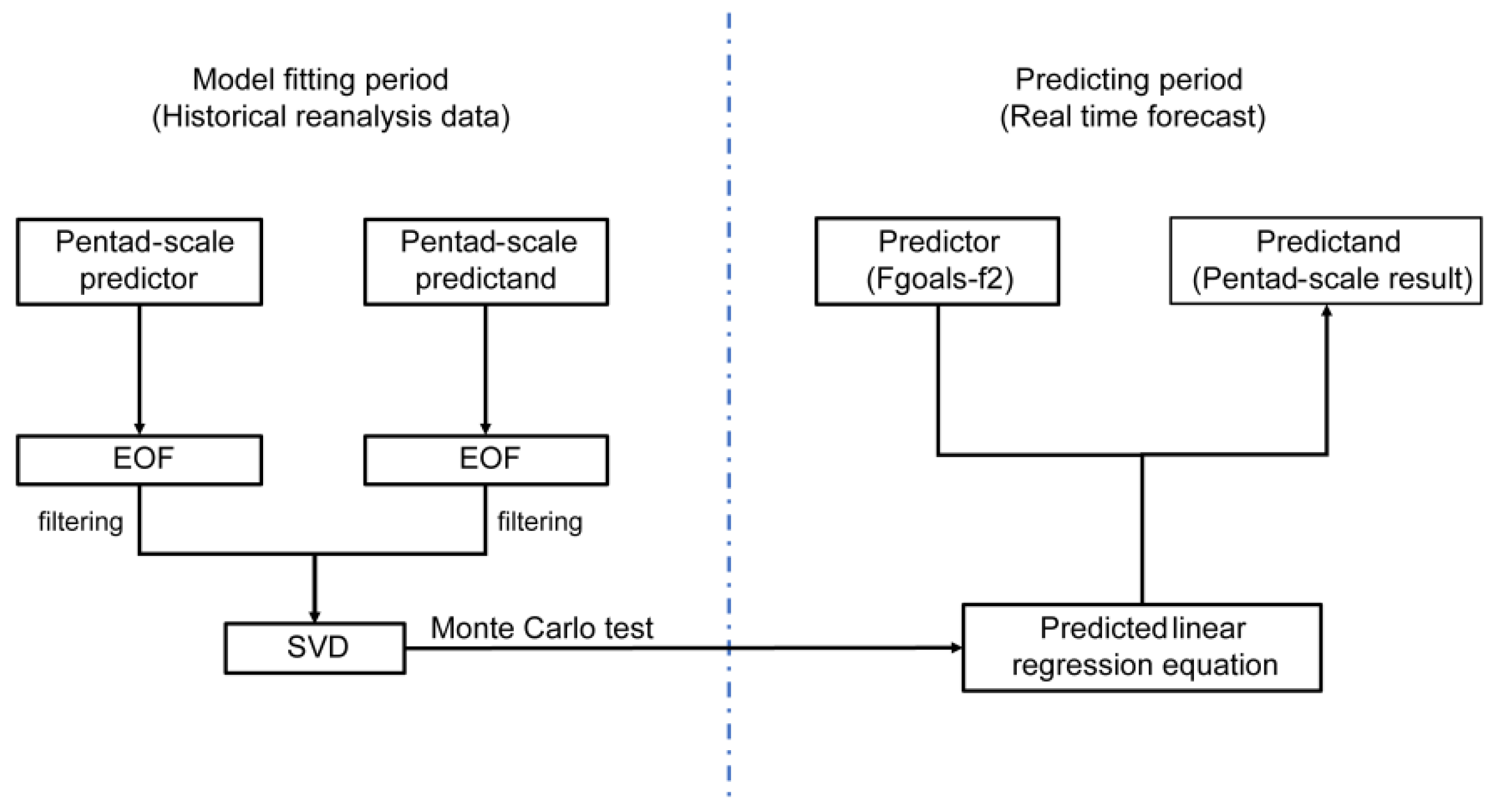
A downscaling method for monthly precipitation prediction was established by Liu and Fan [20]. In order to focus on the pentad-scale precipitation forecast, we established a dynamical–statistical downscaling forecast method on the pentad scale (referred to as a pentad DSDM) for precipitation anomalies via the Z500 anomaly to improve the pentad predictability of precipitation over an extended range (Figure 1). In the pentad DSDM, the SVD downscaling method was used to improve the pentad precipitation forecast based on Z500 from the FGOALS-f2 system and provide a new method for pentad-scale prediction of precipitation. However, only 30 samples were available for each pentad in the 30 years of observed data. We therefore obtained more reanalysis data in the model-fitting period via the moving nine-pentad method (see Section 2.1.1), which resulted in up to 270 available samples for each pentad.

Figure 1.
Flowchart for the pentad DSDM.
The specific steps in the model-fitting period were as follows (Figure 1, left-hand side):
- (1)
- Empirical orthogonal function (EOF) analysis was performed on the historical reanalysis data in the fitting period for each pentad (including precipitation and Z500). For each pentad, the time series of precipitation was reconstructed with its EOF principal components to filter any spatial noise. Only those time series and principal components of the first 90% of contribution variance were retained in the variable reconstruction. The Z500 field was reconstructed in the same way as the precipitation field;
- (2)
- SVD was used to obtain the coupled mode between the predictands and predictors. The coupled SVD modes, the singular values of which were above the noise level, were extracted for each pentad. It is noteworthy that all the singular values of these SVD modes passed the Monte Carlo test [25];
- (3)
- For each pentad, a linear regression equation was established via the coupled SVD time coefficients of the predictands and predictors and then a downscaling prediction model was established for each pentad. A 72 pentad DSDM was therefore established. The SVD of the model-fitting period is shown as Equations (1)–(4).
In the predicting period, after the establishment of the model, the Z500 anomaly predictions of the following 12 pentads were calculated from the FGOALS-f2 model and each initial pentad was used to predict the following 12 pentad precipitation anomalies. For the ith pentad (the initial pentad), the (i + 1)th to the (i + 12)th pentad (the target pentad) could be predicted by the pentad DSDM. For example, taking the pentad of the last pentad of June as the initial pentad, the pentad prediction of the Z500 anomalies was calculated from all the daily Z500 predictions in this pentad (from 26 June to 30 June). The pentad DSDM of the second pentad in July, calculated by the model-fitting period, was then used to predict the precipitation anomalies for the first target pentad and the model of the second pentad in July was used to predict the second target pentad.
In the pentad DSDM, the statistical method was used to establish the relationship between the observed meteorological elements, develop a dynamical–statistical downscaling precipitation forecast model for the extended range and form a set of gridded forecast products with a resolution of 0.5° × 0.5°. As a result of the different resolutions of the datasets used in this study, it was necessary to unify the resolutions of these data to facilitate our calculations. The resolutions of the predictands and predictors were interpolated to 0.5° × 0.5° and 2.5° × 2.5°, respectively, using a bilinear interpolation method.
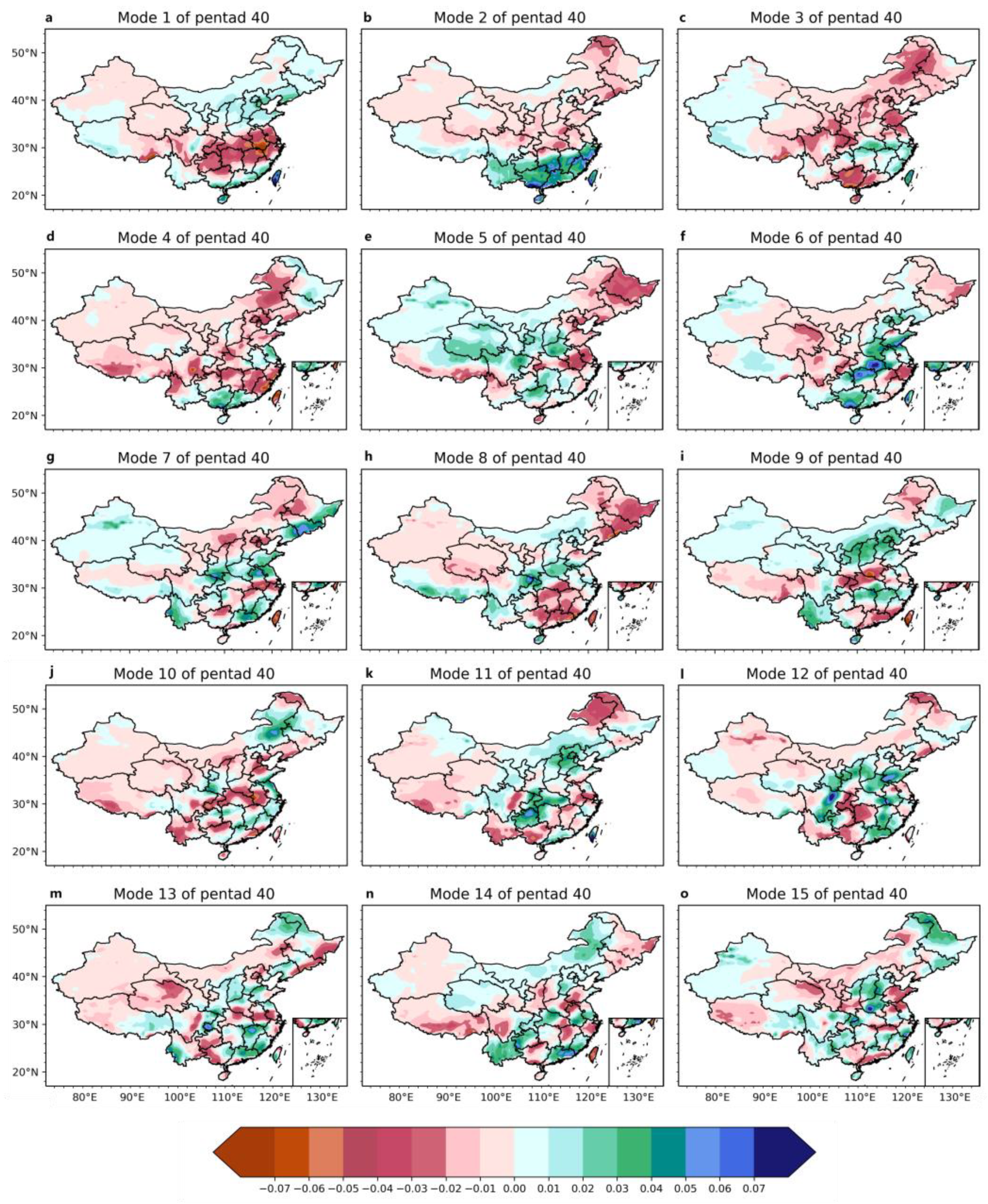
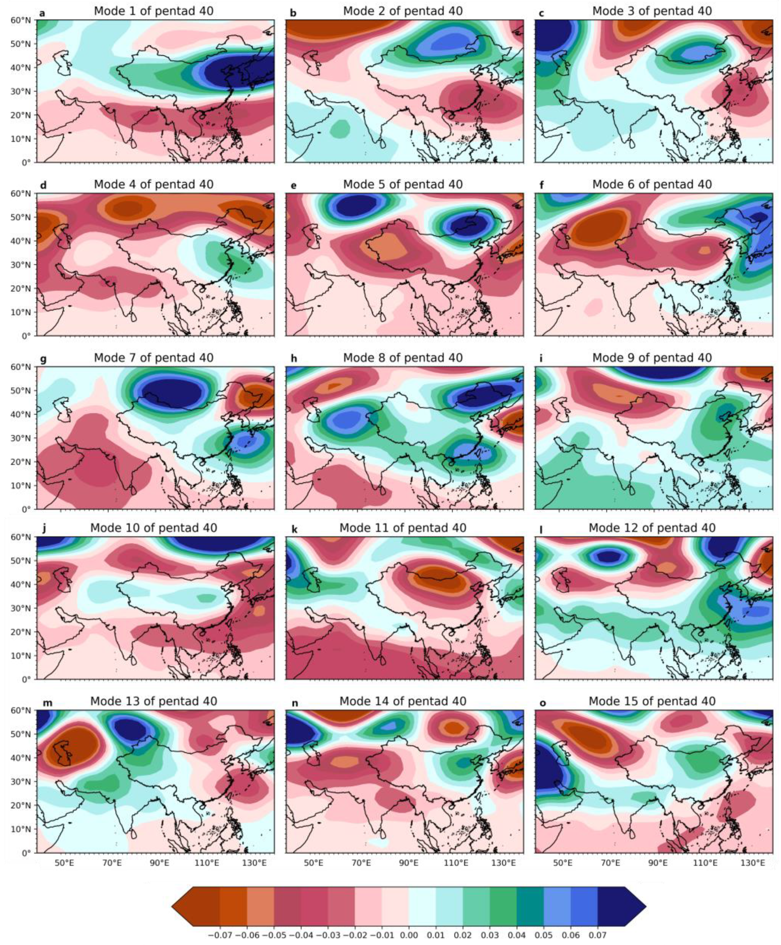
Figure 2 and Figure 3 show the different phase distributions of the Z500 anomalies and the precipitation anomalies in China. For the first mode, when the Z500 anomaly was negative in the area south of 30° N and positive in the area south of 30° N, the precipitation in the areas south of the Yangtze River was lower than the climatological state and vice versa. The rain belt (positive precipitation anomalies) moved northward with the eastward movement of the Z500 anomaly field from the first to the third pentads. The first three coupled patterns, nearly 50% of the total contribution variance, were the dominant patterns in this pentad.
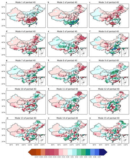
Figure 2.
Left field of the 15 modes (a–o, respectively) of the SVD decomposition (anomaly distribution of the pentad precipitation in the fourth pentad of July).
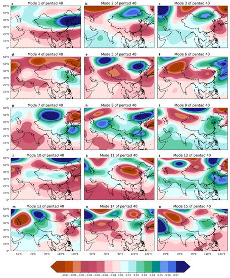
Figure 3.
Right field of the first 15 modes (a–o, respectively) of the SVD decomposition corresponding to Figure 2 (anomaly distribution of the pentad Z500 in the fourth pentad of July).
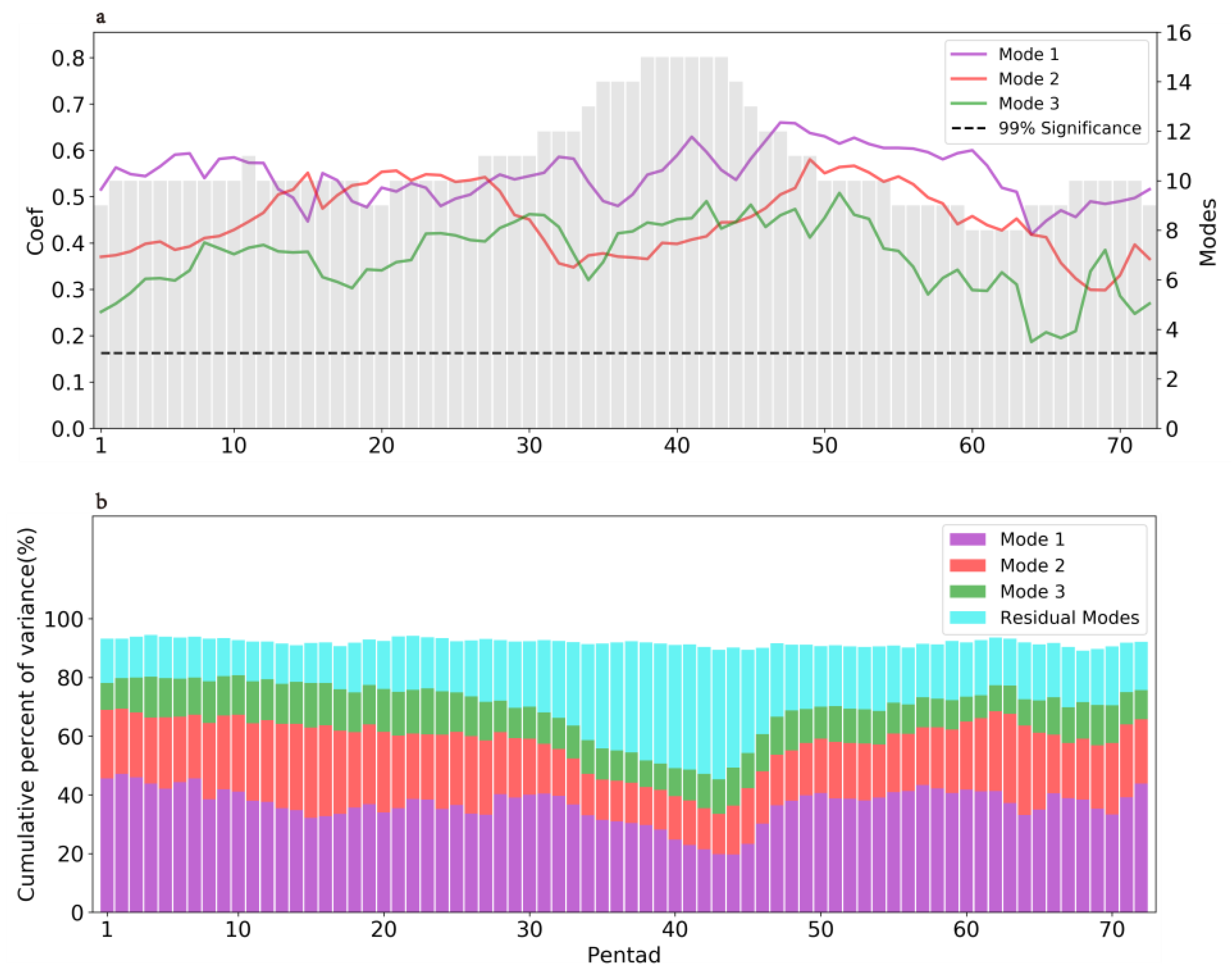
Figure 4 shows the linear regression coefficients () and cumulative percentages of variance for each pentad. All the linear regression coefficients that passed the r-test of 99% significance (the first three modes are shown but the image of the residual modes is omitted) and the number of modes retained via the Monte Carlo test are both shown in Figure 4a. To distinguish statistically significant patterns from random noise, the significant singular value was tested by the Monte Carlo test. Experiments with Gaussian-distributed random data were repeated 100 times and the singular values at a significance level of 99% were obtained using the method developed by Overland and Preisendorfer [25,26]. The cumulative percentages of variance (Figure 4b) showed that most of the variance was about 80% in the first three modes but that, in the summertime, it was relatively lower, about 60%. However, in the DSDM, the modes of each pentad (including the residual modes) are used to predict precipitation. Therefore, more details on the modes can be transferred to make precipitation predictability available in the DSDM.
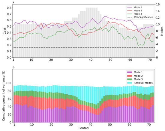
Figure 4.
(a) Linear regression coefficients ( in Equation (3), lines) of the available modes in DSDM (gray bars) and (b) cumulative percentage of variance (%) of the first three SVD modes and the residual modes in the DSDM (the black dotted line denotes the 99% significance test in (a).
2.2.2. Ensemble Average of the Numerical Prediction Model
The ensemble average generally adopts the arithmetic mean of all members under the same weight. The lagged average forecast method can be used to enlarge the ensemble member sample. The ensemble forecast system can reduce the calculation error in chaotic systems (such as the variables of the atmospheric system) [27]. It has been shown that the lagged average forecast method can improve forecasting skills compared to the Monte Carlo method [28]. We applied the lagged average forecast method to the pentad-average anomaly product preprocessed by FGOALS-f2. This product takes the data of the current day and the previous four days as the ensemble members to expand the reforecast ensemble members of the FGOALS-f2 model. The ensemble member samples are therefore enlarged, the algorithm errors caused by some outlier ensemble members are reduced and the stability and predictability of the forecast are improved.
2.3. Evaluation Methods
We used the anomaly correlation coefficient (ACC), the temporal correlation coefficient (TCC) and the mean square skill score (MSSS) as evaluation indices, following the World Meteorological Organization [29].
2.3.1. Anomaly Correlation Coefficient
The ACC reflects the spatial consistency of the model forecast and observations. A time series of the forecast skills for grid points (or stations) can be obtained by calculating the ACC. The value of the ACC ranges from −1 to 1; the larger the value of the ACC, the more consistent the spatial pattern between the forecast and the observations (see Equation (5)).
2.3.2. Temporal Correlation Coefficient
The TCC reflects the model predictability of the anomalies for each grid point (or station) statistically. The value of the TCC ranges from −1 to 1; the larger the value of the TCC, the better the forecast ability of the model under the same forecast time period (see Equation (6)).
2.3.3. Mean Square Skill Score Index
The MSSS index is the ratio of the forecast error to the “climate” forecast error. The closer the MSSS value is to 1, the more accurate the prediction of the model. An MSSS greater than zero indicates that the model forecast is meaningful. We focus here on the prediction of anomalies rather than the deviation of the climatological state in the forecast, so the drift of the climatological state is not considered when calculating the forecast error. The formula of the forecast mean squared error is shown in Equations (7)–(10).
2.3.4. Regional Average
The effects of latitude should be considered when calculating the evaluation score of an area. The grid points at different latitudes therefore have different weights; for example, the regional mean TCC is defined in Equation (11).
2.4. Formatting of Mathematical Components
For each pentad:
where M is the pattern number passing the Monte Carlo test. and are the time expansion coefficients of ith SVD mode for the predictand and predictor, respectively, and and are their singular vectors. is the linear regression coefficient for the ith coupled pattern.
For the target pentad (the pth pentad), the precipitation prediction can be expressed as:
where
The mean squared error of the climatological forecast is:
and, therefore, the MSSS is defined as:
where wi is the weight of different latitudes. The calculation method for the regional mean MSSS is the same as that for the TCC.
3. Evaluation of the Pentad DSDM
3.1. Evaluation of the Pentad DSDM Precipitation Reforecast
Based on the Z500 data from FGOALS-f2, we predicted the precipitation pentad anomaly using pentad DSDM. We used the statistical verification index of the ACC, TCC and MSSS to compare the predictability of the FGOALS-f2 model and the pentad DSDM for whole years and for summertime from 2000 to 2018.
3.1.1. ACCs for Precipitation Forecast
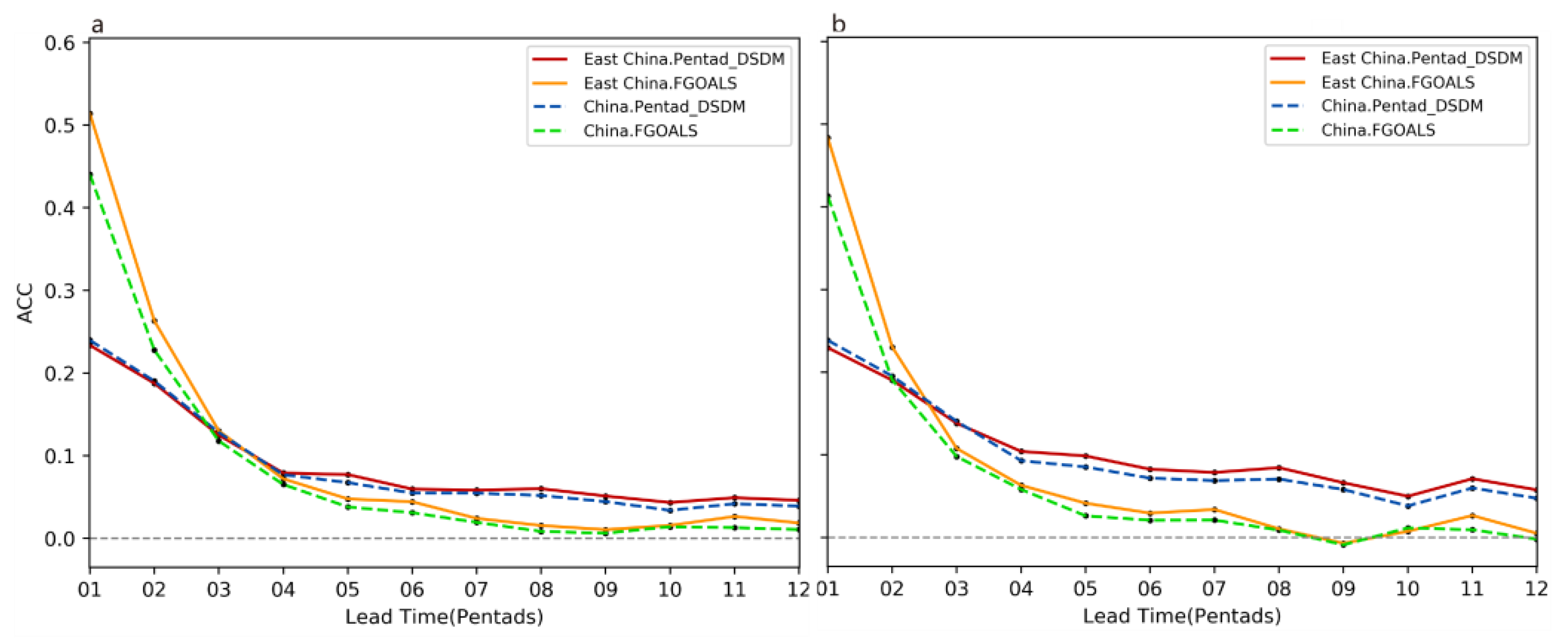
The ACC values of the FGOALS-f2 model and the pentad DSDM for the precipitation forecast at lead times of 1 to 12 pentads were both greater than zero, which indicates that these two models are both capable of predicting the distribution of precipitation in China. The FGOALS-f2 model has higher forecasting skills than the pentad DSDM for forecasting pentads 1 to 2. At a lead time of one pentad, the ACC values of the FGOALS-f2 model were twice those of the pentad DSDM for forecasting precipitation in China. With an increase in the lead time, the ACCs of both these two models for the forecast of precipitation decreased significantly, but the ACCs of the pentad DSDM decreased more slowly than the ACCs of the FGOALS-f2 model (Figure 5a, blue and green dotted lines).
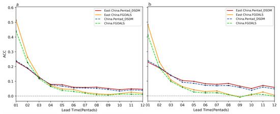
Figure 5.
ACCs of the precipitation anomalies forecast from 2000 to 2018 for the pentad DSDM and FGOALS-f2 model. (a) The annual average (from the first pentad in January to the sixth pentad in December) and (b) the summer average (from the first pentad in June to the sixth pentad in August).
The ACC values of the FGOALS-f2 model and the pentad DSDM for precipitation forecast were close at a lead time of four pentads. The forecasting skill of the pentad DSDM gradually became higher than that of the FGOALS-f2 model as the lead time increased. The ACCs of the pentad DSDM remained almost unchanged with an increase in the lead time, whereas the forecasting skill of the FGOALS-f2 model continued to decrease, which indicates that the pentad DSDM has a higher forecasting skill than the FGOALS-f2 model. The ACC scores show that the precipitation of the FGOALS-f2 model was more meaningful than the pentad DSDM at a lead time of two pentads and the ACC scores decreased rapidly with the lead time. The pentad DSDM gave a better prediction for forecasts with a lead time longer than four pentads. Table A1 (see Appendix A) shows that the mean ACC scores of FGOALS-f2 were less than 0.04 after a lead time of five pentads, whereas those of the pentad DSDM were about 0.04.
In the comparison of the ACCs at different lead times (Figure 5), the FGOALS-f2 model showed poorer predictability during the summer than over the whole year. The ACC scores of both models were negative at lead times of nine pentads in summer and the ACCs of the FGOALS-f2 model were smaller than those of the pentad DSDM. In contrast, the pentad DSDM, based on Z500, showed a higher predictability in summer than over the whole year. The precipitation prediction ACC scores of the pentad DSDM were greater than those of FGOALS-f2 at leads time longer than four pentads averaged over the whole year (Figure 5a) and at lead times longer than three pentads for the summer average (Figure 5b). This indicates that the downscaling model can improve the poor predictability of FGOALS-f2 at lead times longer than three pentads. The pentad DSDM therefore shows a higher predictability than FGOALS-f2 for the prediction of precipitation at lead times from 3 to 12 pentads, which further suggests that the pentad DSDM is more suitable for forecasts of summer precipitation.
3.1.2. TCCs for Precipitation Forecasts
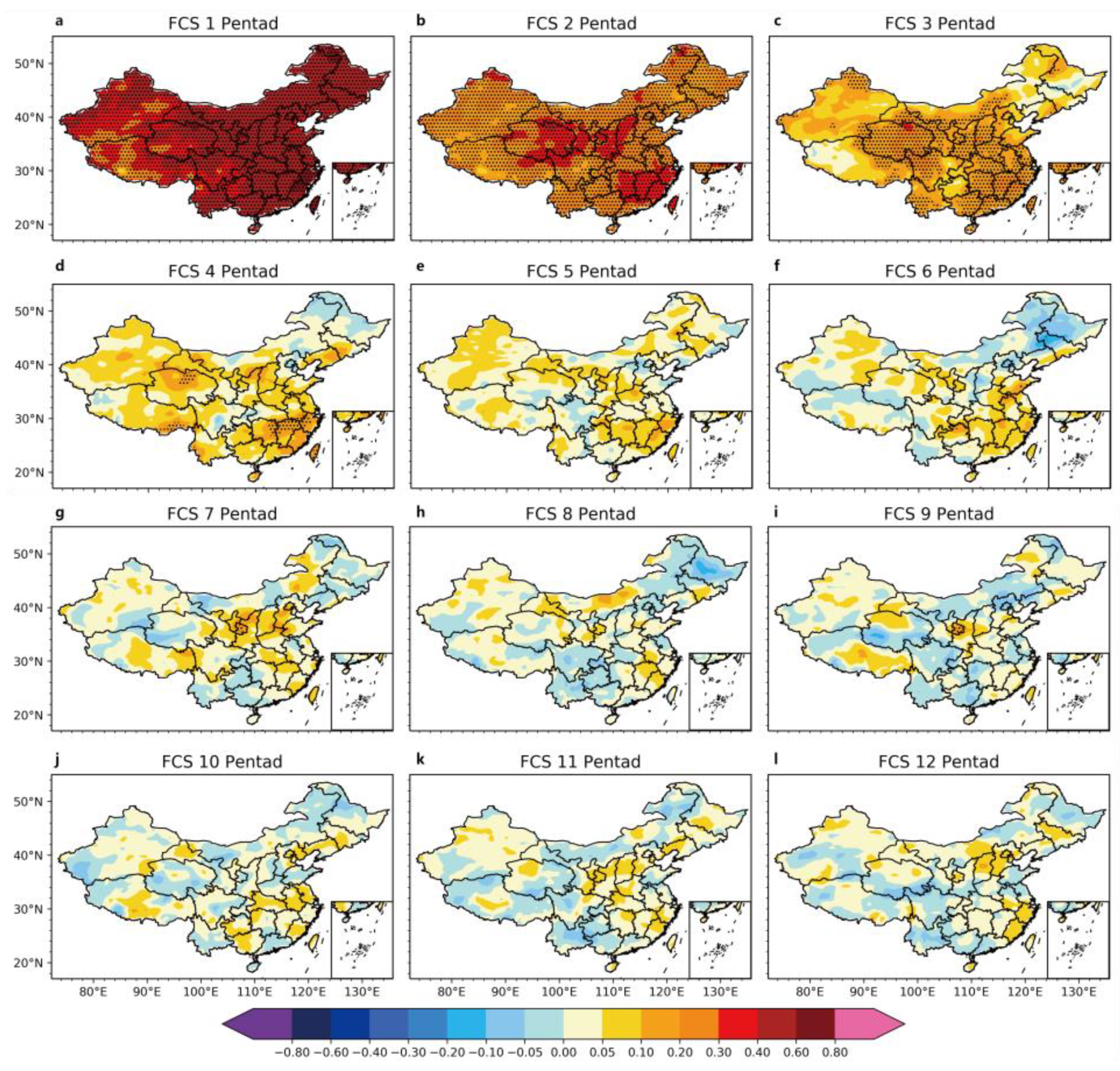
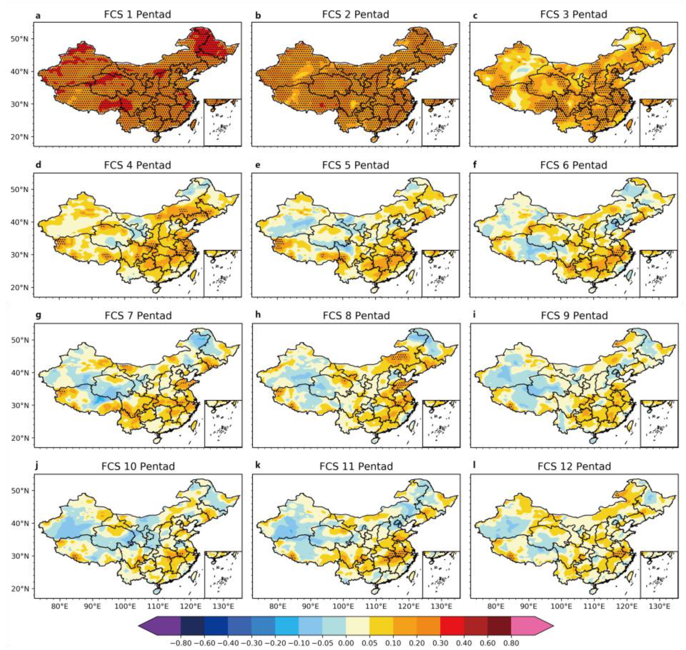
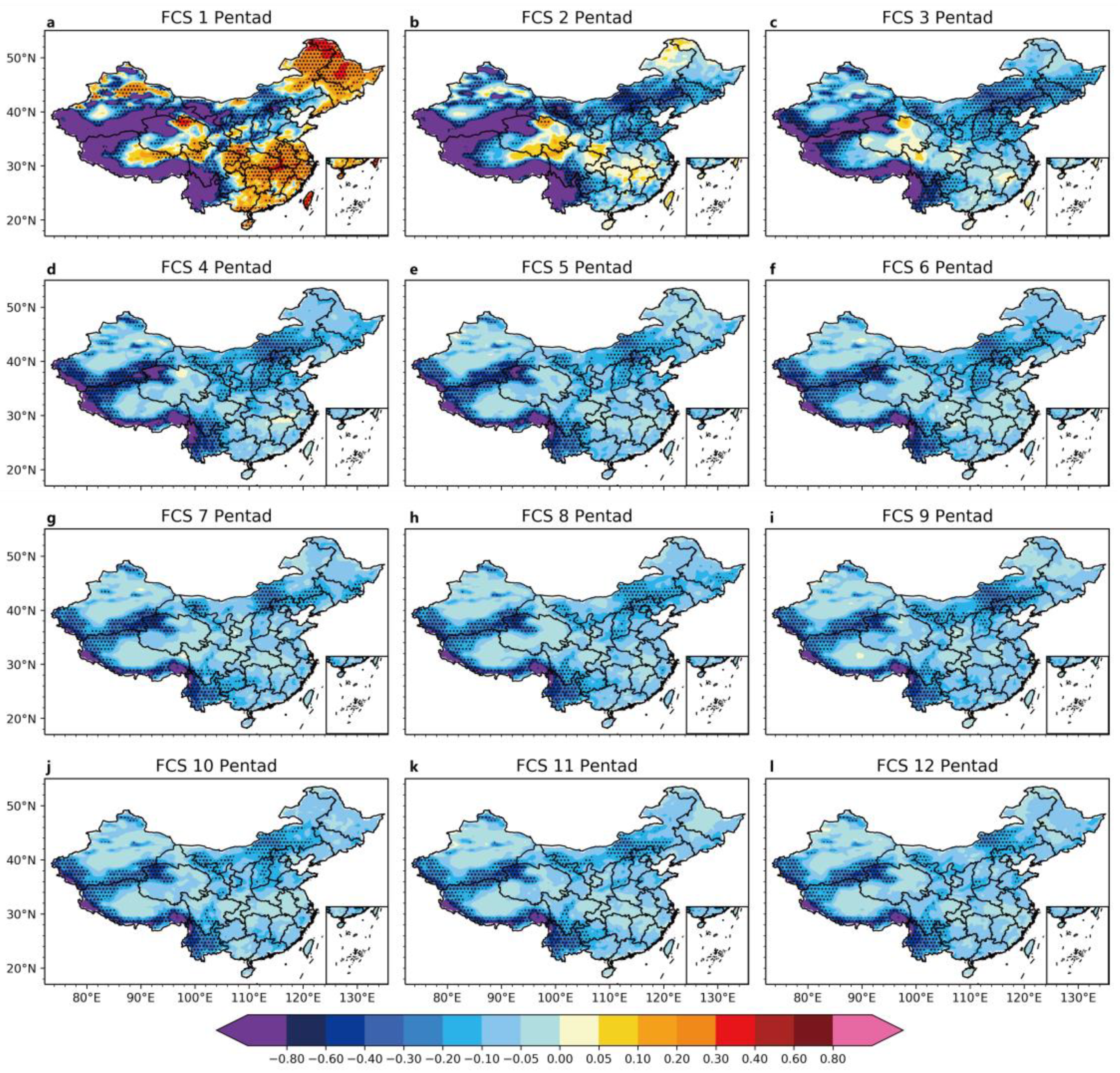
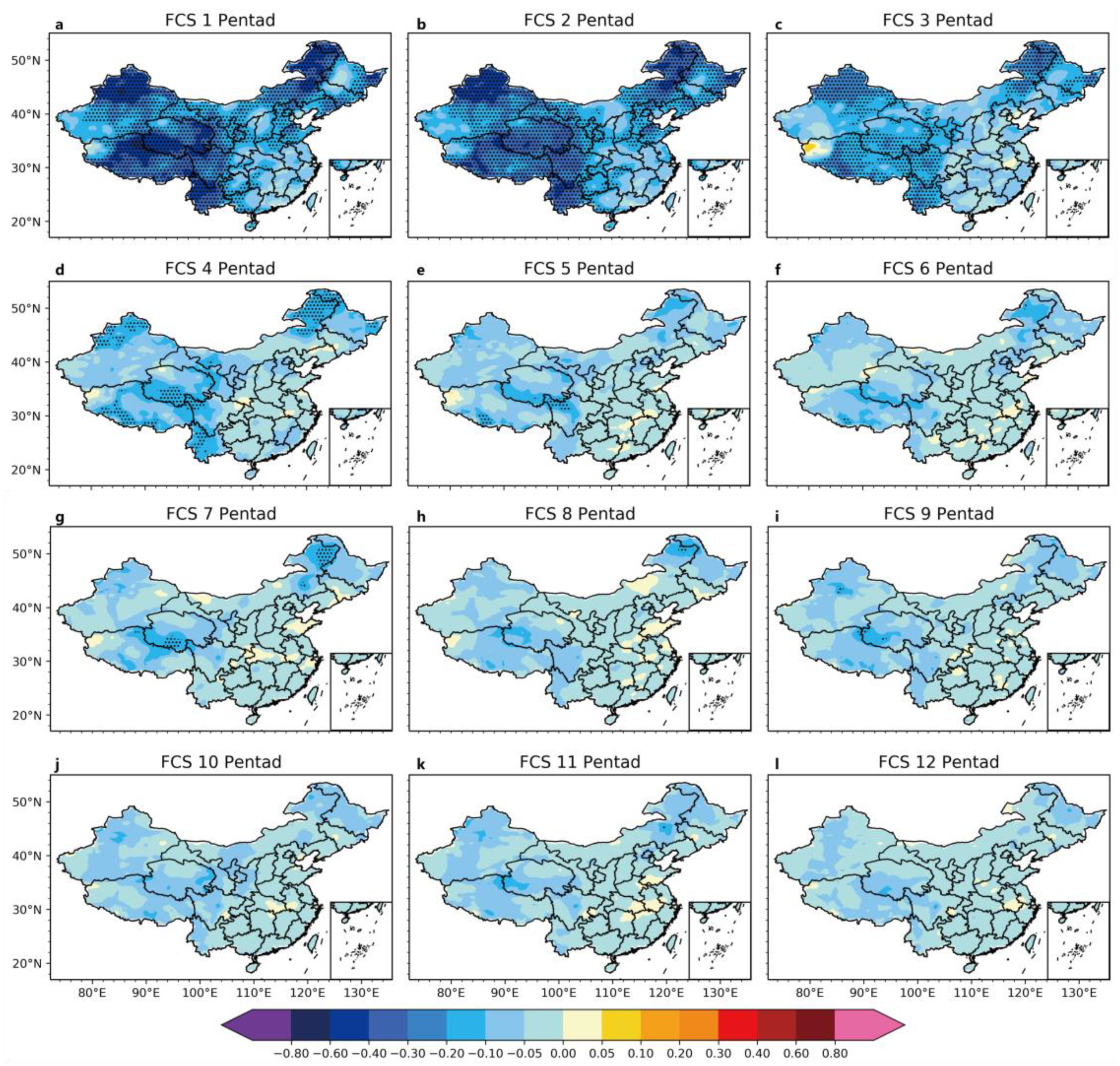
The TCCs of the pentad DSDM decreased significantly with the increase in the lead time compared with the one- to six-pentad precipitation forecasts in China (Figure 6 and Figure 7). The TCC values of the pentad DSDM were lower than those of the FGOALS-f2 model at lead times of one to three pentads. However, the advantages of the precipitation forecasts using the pentad DSDM gradually emerged for forecasts at lead times longer than four pentads in most areas of China, especially in south China, the Yangtze River basin and southwest China. The precipitation prediction TCCs of the pentad DSDM showed a clear decreasing trend with increasing lead time in northwest China, the plateau regions and northeast China, with TCC values less than zero at lead times greater than three pentads. Considering the similarity with the historical precipitation, the areas where the TCCs passed the 95% significance test with a degree of freedom of 216 (but not the 19 year degree of freedom of 1368) are shown as dotted regions in Figure 6 and Figure 7. These results demonstrate the more significant achieved with the pentad DSDM. The MSSS skill scores used the same significant r-test.
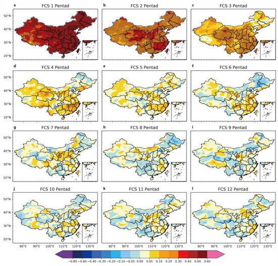
Figure 6.
Spatial pattern of the annual average TCC for the leading 1–12 (a–l, respectively) pentad precipitation forecast of the FGOALS-f2 model from 2000 to 2018. The dotted regions are where the TCC passed the 95% significance test.
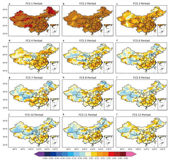
Figure 7.
Spatial pattern of the annual average TCC for the 1–12 (a–l, respectively) pentad precipitation forecast of the pentad DSDM from 2000 to 2018. The dotted regions are where the TCC passed the 95% significance test.
Figure 6g–l show that the changes in the TCC values were not significant with increasing lead times, which means that the pentad DSDM had a better forecast stability at lead times of 7 to 12 pentads. For the forecasts at lead times of one to six pentads, the TCCs decreased significantly with the lead time over northwest China, the plateau region and northeast China. The TCC values were between 0 and −0.1 for lead times from 7 to 12 pentads. The downward trend at lead times of 7 to 12 pentads was less obvious than that at lead times from one to six pentads. Compared to the FGOALS-f2 model, the pentad DSDM showed a significant improvement in forecasting skill at lead times of 7 to 12 pentads, especially in the important region of east China.
The precipitation forecast at lead times of one and two pentads passed the significance test nationwide, indicating that the FGOALS-f2 model gave a credible forecast during the first two pentads. The TCC values in the area where the models results passed the significance test began to decrease at lead times of three and four pentads. However, for precipitation forecasts with a lead time longer than five pentads, the TCCs of the areas passing the significance test in the pentad DSDM were larger than in the FGOALS-f2 model. These areas were mainly located in the eastern coastal areas of China and the downstream areas of the Yangtze and Yellow rivers. It is therefore necessary to use the dynamical–statistical downscaling model for the correction of precipitation forecasts in the eastern coastal area for forecasts longer than five pentads.
The average forecast skill in China of both the pentad DSDM and the FGOALS-f2 model decreased with increasing lead times (pentads), which reflects the relationship between the forecast time and the predictability of current model forecasts. However, the average TCCs and ACCs of the FGOALS-f2 model decreased rapidly with the increase in the lead time, and the forecasting skill scores of the FGOALS-f2 model were lower than those of the pentad DSDM at lead times longer than four pentads. The pentad DSDM therefore showed an improvement in precipitation forecast skill at lead times longer than four pentads (Table 1).

Table 1.
Skill scores averaged over the whole of mainland China.
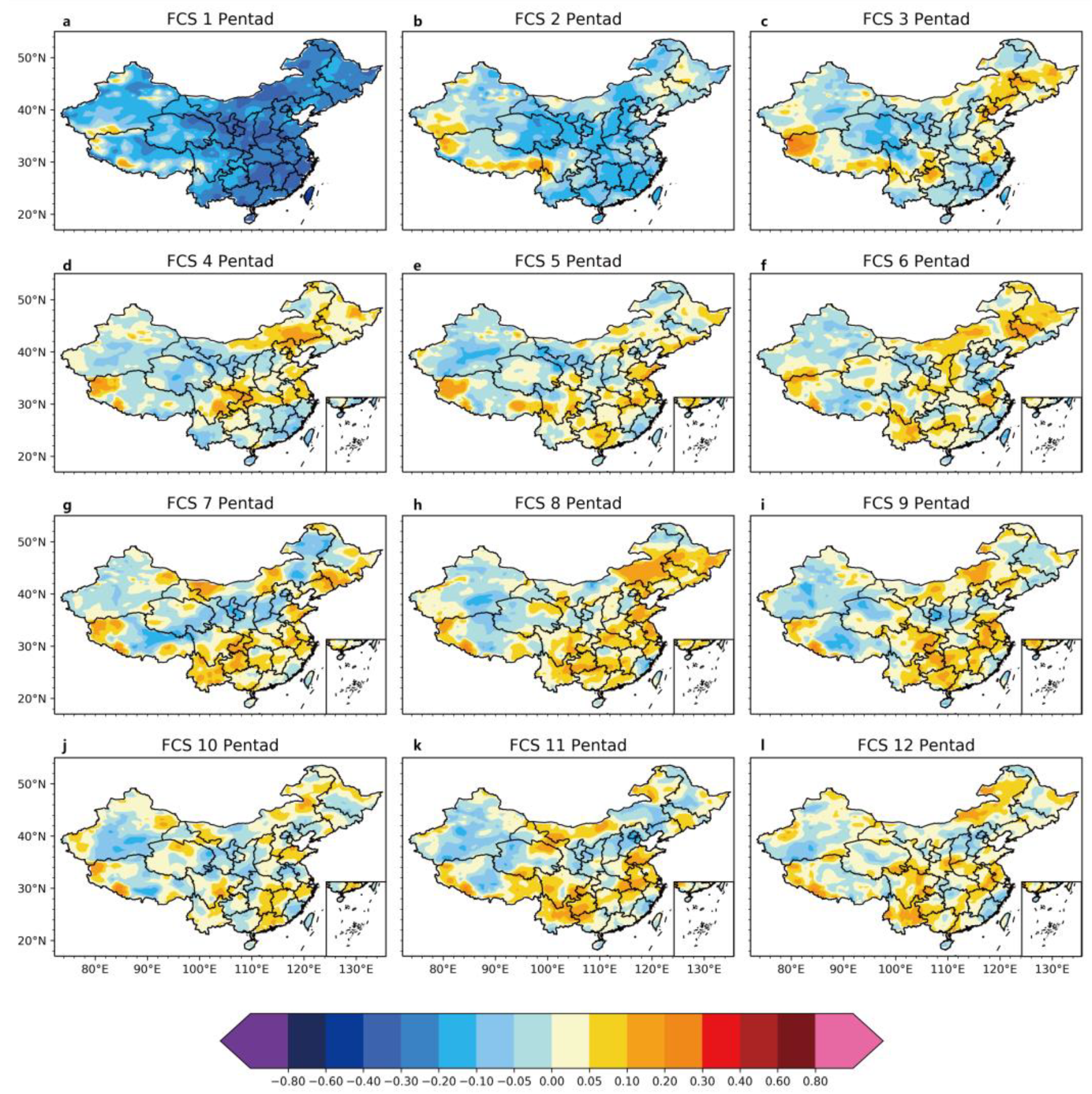
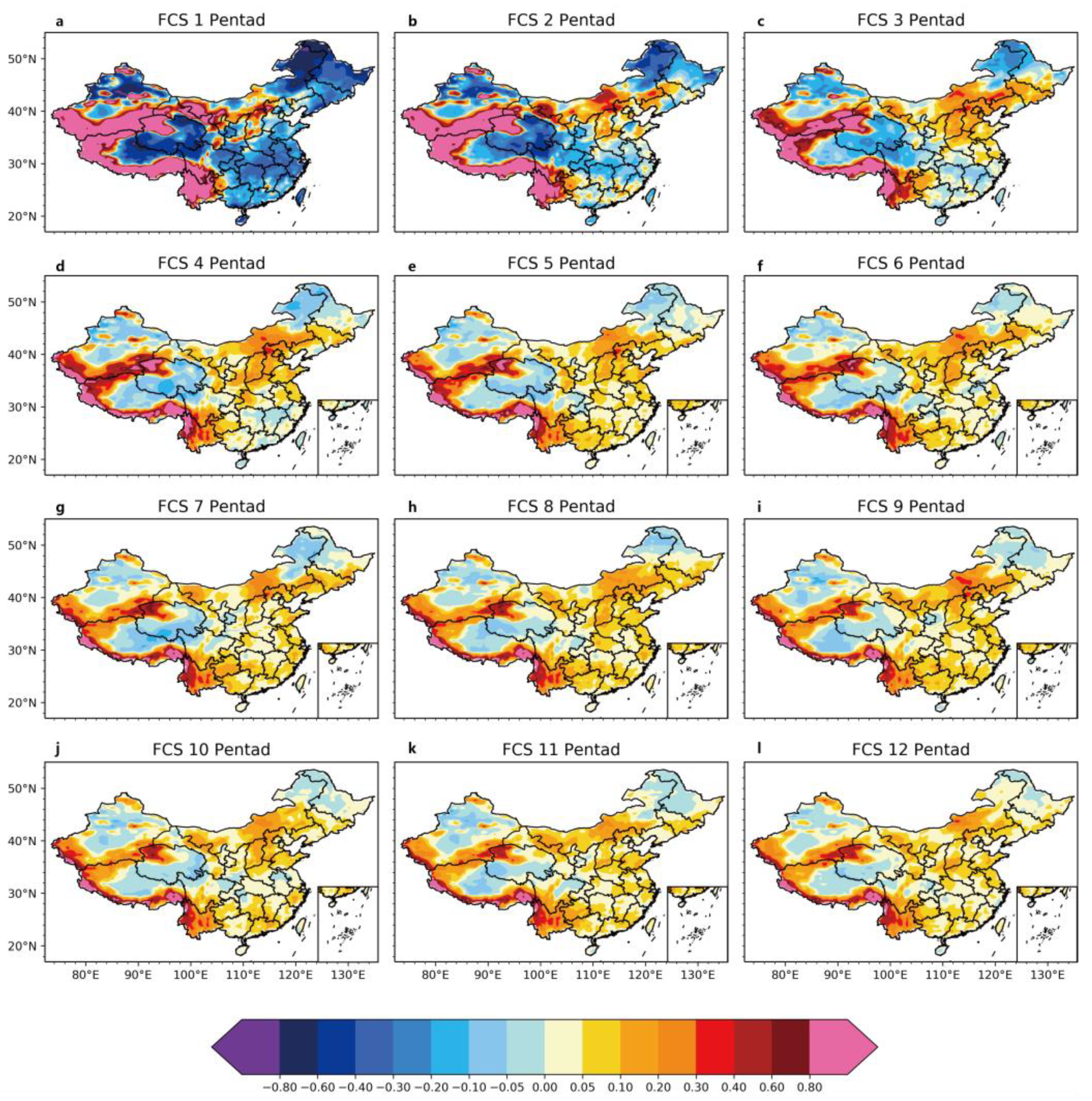
The differences in the TCCs (the pentad DSDM minus the FGOALS-f2 model) (see Figure 8) reflected the differences in the spatial predictability of precipitation between the FGOALS-f2 model and the pentad DSDM. The positive values indicate where the pentad DSDM was better than the FGOALS-f2 model and vice versa. In the first two lead pentads, the TCC differences were almost negative for the whole of China, meaning that the FGOALS-f2 model had a higher forecasting skill than the pentad DSDM, which was also reflected in the ACC scores. For forecasts at lead times longer than three pentads, the area of positive TCC differences increased with the lead pentads. The positive area in eastern China was larger than that in western China, which means that better prediction of precipitation at lead times longer than three pentads can be obtained with the pentad DSDM.

Figure 8.
Spatial pattern of the annual average TCC differences (pentad DSDM minus FGOALS-f2) between the pentad DSDM and the FGOALS-f2 model for the 1–12 (a–l, respectively) pentad precipitation forecast from 2000 to 2018.
3.1.3. MSSSs for Precipitation Forecasts
Compared with the MSSSs of the pentad DSDM for precipitation forecasts over China at lead times of one to six pentads (Figure 9), the MSSSs decreased significantly with increasing lead times. Although the forecast skill of the pentad DSDM was not as good as that of the FGOALS-f2 model at lead times of one to three pentads, the MSSSs of the FGOALS-f2 model showed a significant downward trend with increasing lead times. The advantage of the pentad DSDM prediction gradually appeared at lead times longer than four pentads. In addition, the MSSSs of the four- to six-pentad precipitation forecasts of the pentad DSDM were higher than those of the FGOALS-f2 model in most areas of China, especially in south China, the Yangtze River basin and southwest China, which are greatly affected by precipitation.
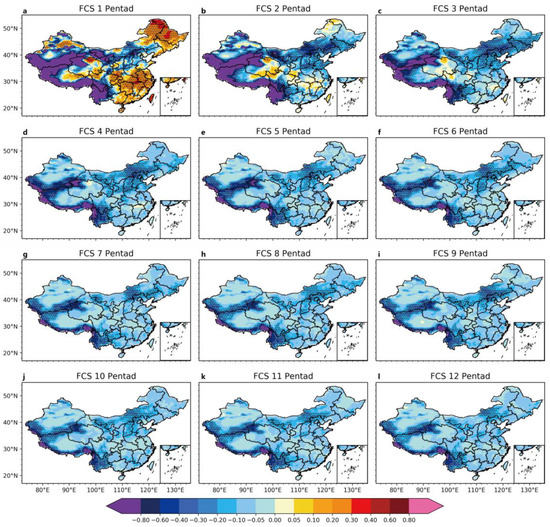
Figure 9.
Spatial pattern of annual average MSSS for the 1–12 pentad (a–l, respectively) precipitation forecast of the FGOALS-f2 model from 2000 to 2018. The dotted regions are where the MSSS passed the 95% significance test.
However, Figure 10 shows that the MSSSs did not change significantly with the lead time, which means that pentad DSDM had a better forecast stability at lead times of 7 to 12 pentads. For one- to six-pentad prediction, in the area where the MSSSs decreased significantly with the lead time (e.g., northwest China, the plateau regions and the northern part of northeast China), the MSSSs were less than zero and the changes were not significant with increasing lead times. Compared with the MSSSs of the FGOALS-f2 model, the pentad DSDM showed a more significant improvement at lead times of 7 to 12 pentads and the forecast skills were more stable.

Figure 10.
Spatial pattern of annual average MSSS for the 1–12 (a–l, respectively) pentad precipitation forecast of the pentad DSDM from 2000 to 2018. The dotted regions are where the MSSS passed the 95% significance test.
The MSSS differences (the pentad DSDM minus the FGOALS-f2 model) (Figure 11) indicated similar conclusions as the TCC differences. In addition, the pentad DSDM showed better performance in eastern China after a lead time of five pentads. However, the precipitation in the Tibetan Plateau was difficult to predict with both the FGOALS-f2 model and the pentad DSDM.
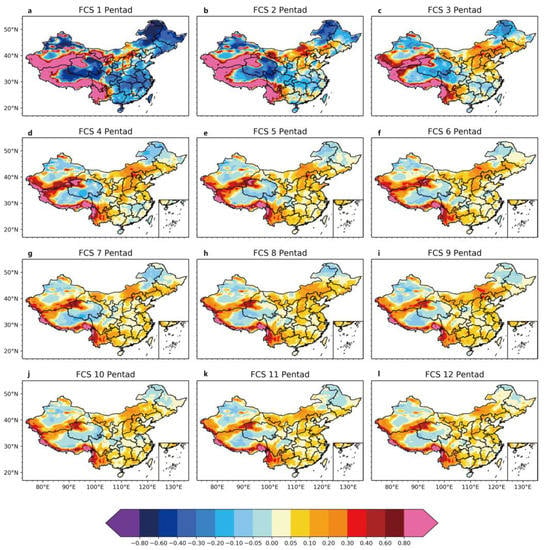
Figure 11.
Spatial pattern of the annual average MSSS differences (pentad DSDM minus FGOALS-f2) between the pentad DSDM and the FGOALS-f2 model for the 1–12 (a–l, respectively) pentad precipitation forecast from 2000 to 2018.
4. Reforecast Analysis of the Zhengzhou “720” Super Heavy Rainstorm Event
The torrential rainstorm from 18 to 22 July 2021 was one of the heaviest rainfall events ever recorded in Zhengzhou. The rain caused many dangerous dike collapses in urban areas, affected more than 1.88 million people and led to economic losses of 5.32 million yuan. Figure 12a shows that the precipitation at the third pentad of July 2021 was lower in the southern area (south of 30° N) than in the north (north of 30° N). In addition, there were two centers of positive precipitation anomalies: one in northeastern Sichuan and southern Gansu and the other in the Huaihe–Haihe river basin. Figure 12b shows that the center of the negative precipitation anomaly moved to the southwestern area in the fourth pentad of July. The rain belt then moved northward and another center of positive precipitation anomalies appeared in Zhejiang in the fifth pentad of July (Figure 12c).

Figure 12.
Precipitation anomalies in China for the (a) third pentad of July 2021 (11–15 July), (b) fourth pentad of July 2021 (16–20 July) and (c) fifth pentad of July 2021 (21–25 July).
Comparison between Observations and Model Forecasts
The spatial distribution of precipitation in the third pentad of July 2021 (initial pentad: the last pentad of June; Figure 13a,d) in the FGOALS-f2 precipitation forecast was consistent with that from the observations south of 30° N but did not capture the center of the negative precipitation anomaly north of 30° N. This is consistent with a previous study of the S2S forecast (the significant correlation in the forecast skill is limited to week 1, about two pentads) [7]. The pentad DSDM was more consistent with the observations than the FGOALS-f2 model, especially in eastern China. The FGOALS-f2 model showed the opposite precipitation anomalies to the observations in the fourth pentad of July 2021 and also had poor predictability in the fifth pentad of July 2021 (Figure 13b,c). In contrast, with the same lead times of four and five pentads, respectively, the centers of the positive precipitation anomalies via the pentad DSDM were consistent with the observations (Figure 13e,f). Although the occurrence of extreme precipitation events cannot be well predicted by the pentad DSDM, the area and migration of rain belts in extreme rainfall events can be well predicted at lead times from three to five pentads. The pentad DSDM can therefore capture more signals by steadily predicting Z500, and it turns the signals into better predictions than FGOALS-f2 precipitation prediction (three or more pentads).
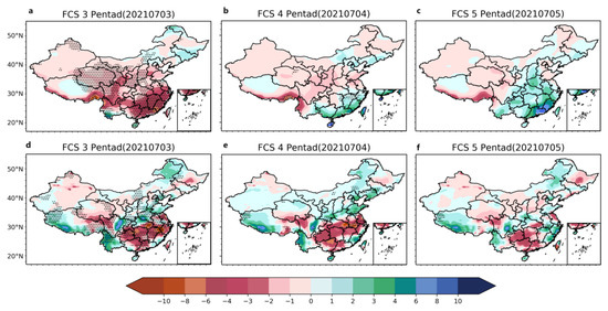
Figure 13.
Spatial patterns of the (a–c) FGOALS-f2 and (d–f) pentad DSDM forecasts from the third to fifth pentads of July 2021 (the initial pentad was the last pentad of June 2021 (26–30 June). The dotted areas indicate that the TCC passed the 95% significance test.
Table 2 analyzes the mechanism of the pentad DSDM using projection coefficients. In the fourth pentad of July 2021, predicted by the last pentad of June 2021, the projection coefficients of the 1st, 4th, 8th and 11th patterns were much larger than other coefficients. The fourth and first precipitation patterns were both consistent with the results of the pentad DSDM (Figure 13e). The Z500 anomalies (Appendix A, Figure A1b) prove that the Z500 anomalies were consistent with the first pattern, although the fourth pattern with a positive projection coefficient and the 8th and 11th patterns with negative projection coefficients are difficult to explain. Hence, a better result was obtained when there was no significant difference in the magnitudes of the multiple projection coefficients, which means that multiple coupled patterns work together, but this is difficult to explain. Surprisingly, when we used the patterns that passed the Monte Carlo test, they were not only able to capture the large-scale Z500 signals (such as the fourth and first coupled patterns mentioned above) but also obtained better results than the other signals with a low contribution to the variance.

Table 2.
Projection coefficient of the fourth pentad of July 2021 predicted by pentad DSDM in the predicting period (initial pentad: last pentad of June 2021).
The pentad DSDM captured the variable relationship between Z500 and the precipitation anomalies in summer via the spatial modes of the SVD decomposition and it showed better results than the FGOALS-f2 model. Likewise, the relationship between the precipitation in east China (east of 110° E) and the Z500 anomaly was captured better by the pentad DSDM. The pentad DSDM was therefore more accurate than the FGOALS-f2 model in predicting precipitation anomalies at lead times longer than four pentads (and even three pentads in summer). In addition, in east China, where the precipitation patterns are complex and changeable, the changes in the circulation and precipitation could be captured by the pentad DSDM, which provided more accurate information for pentad-scale precipitation forecasting than the FGOALS-f2 model.
5. Discussion and Conclusions
We established a pentad DSDM based on the relationship between the Z500 anomaly and precipitation anomalies in China. We evaluated the statistical downscaling model using the ACC, TCC and MSSS and carried out a qualitative analysis of the model through event analysis. Our conclusions are as follows:
- (1)
- At lead times longer than four pentads (three pentads in summer), the pentad DSDM could effectively make up for the rapid decrease in the sub-seasonal precipitation predictability of the FGOALS-f2 model at increased lead times. With lead times greater than four pentads, the ACCs, TCCs and MSSSs of the pentad DSDM for the whole of China were higher than those of the FGOALS-f2 model;
- (2)
- In the reforecast analysis of the Zhengzhou “720” super heavy rainstorm event, the area and migration of the rain belts were predicted well by the pentad DSDM at lead times of three pentads;
- (3)
- The pentad DSDM could better predict summer precipitation in the eastern coastal areas of China at lead times of three pentads or longer by capturing the changes in the Z500 circulation of the FGOALS-f2 model;
- (4)
- The coupling signals between the Z500 anomalies and the precipitation anomalies could be retained by taking all the coupled SVD patterns that passed the Monte Carlo test to construct the pentad DSDM for each pentad. This led to better predictability in the extended range.
Daily forecasts are not feasible for periods of six to ten days and the skill of the model system is limited to two weeks. Some studies have therefore tried to improve the S2S forecast in the corrected model [9,30]. Zheng Lu [15] applied the statistical downscaling model to the Climate Forecast System version 2 (CFSv2) and the CFSv2 model improved the forecast of station rainfall in south China, with the average TCCs increasing from 0.14 to 0.31. This was also shown in the statistical downscaling model with lead times greater than four pentads in our study (Figure 6 and Figure 7). In addition, the TCCs increased to >0.1 and even 0.2 in most of eastern China using multiple patterns. Our study therefore shows the ability and potential of pentad prediction of anomalous precipitation (Figure 8). Pentad-scale prediction can keep the daily forecast as accurate as possible and has a higher time resolution than monthly prediction.
The pentad DSDM based on the Z500 circulation of the FGOALS-f2 model had better predictability of precipitation than the FGOALS-f2 model at lead times of three or more pentads, especially in summer. However, in other seasons, the increasing skill score was not as significant as in summer. It is therefore necessary to find more suitable predictors for the pentad-scale precipitation and the optimum combination of predictors to construct a multi-factor model; this is the key to future research. The pentad DSDM can capture more features for precipitation prediction by incorporating more predictors, thereby increasing the predictive ability of pentad precipitation and filling the gap between traditional weather forecasting and short-term climate prediction. In addition, the daily scale of weather forecasts, the pentad scale of S2S or extended range forecasts and the monthly scale of short-term climate prediction may fill the prediction gaps at different timescales.
Author Contributions
Conceptualization, H.C. and J.Z.; methodology, Z.Z.; software, Z.Z. and H.C.; validation H.L., J.Z. and H.C.; formal analysis, W.L. and J.Z.; investigation, H.C. and W.L.; resources, W.L., J.Z. and H.L.; data curation, H.C.; writing—original draft preparation, H.C. and W.L.; writing—review and editing, H.C. and H.L.; visualization, H.C. and Z.Z.; supervision, H.C. and J.Z.; project administration, H.L. and W.L.; funding acquisition, H.L., W.L. and J.Z. All authors have read and agreed to the published version of the manuscript.
Funding
This study was jointly supported by the National Key Research and Development Program of China (2021YFC3000902), the National Natural Science Foundation of China (42075087, U20A2097) and Guangzhou Meteorological Society Science and Technology Research Project (M202105).
Institutional Review Board Statement
Not applicable.
Informed Consent Statement
Not applicable.
Data Availability Statement
Data sets for this research are publicly available. Archives of meteorological parameter data are available at: S2S data of IAP-CAS (FGOALS-f2). https://apps.ecmwf.int/datasets/data/s2s-reforecasts-instantaneous-accum-anso/levtype=sfc/type=cf (accessed on 20 March 2022). NCEP/NCAR Reanalysis 1. https://psl.noaa.gov/data/gridded/data.ncep.reanalysis.html (accessed on 12 December 2021). CRA-40 from National Meteorological Information Centre. http://www.nmic.cn (accessed on 25 December 2021).
Acknowledgments
Not applicable.
Conflicts of Interest
The authors declare no conflict of interest.
Appendix A

Table A1.
ACC scores for each leading pentad over China (the rate of increase was calculated using Equation (A1)).
Table A1.
ACC scores for each leading pentad over China (the rate of increase was calculated using Equation (A1)).
| Lead Time (Pentad) | Pentad DSDM (ACC) | FGOALS-f2 (ACC) | Rate of Increase (%) |
|---|---|---|---|
| 1 | 0.240 | 0.440 | −45.6 |
| 2 | 0.190 | 0.228 | −16.5 |
| 3 | 0.128 | 0.118 | 8.6 |
| 4 | 0.077 | 0.065 | 18.3 |
| 5 | 0.068 | 0.038 | 77.8 |
| 6 | 0.055 | 0.031 | 76.2 |
| 7 | 0.054 | 0.019 | 181.8 |
| 8 | 0.052 | 0.008 | 520.3 |
| 9 | 0.045 | 0.006 | 633.7 |
| 10 | 0.034 | 0.014 | 142.2 |
| 11 | 0.042 | 0.013 | 227.0 |
| 12 | 0.039 | 0.011 | 269.0 |

Figure A1.
Prediction of the Z500 anomalies using the (a) third pentad of July 2021 (11–15 July), (b) fourth pentad of July 2021 (16–20 July) and (c) fifth pentad of July 2021 (21–25 July).
Figure A1.
Prediction of the Z500 anomalies using the (a) third pentad of July 2021 (11–15 July), (b) fourth pentad of July 2021 (16–20 July) and (c) fifth pentad of July 2021 (21–25 July).

References
- Zheng, Z.; Huang, J.; Feng, G.; Chou, J. Forecast scheme and strategy for extended-range predictable components. Sci. China Earth Sci. 2012, 56, 878–889. [Google Scholar] [CrossRef]
- Reichler, T.J.; Roads, J.O. The role of boundary and initial conditions for dynamical seasonal predictability. Nonlinear Process. Geophys. 2003, 10, 211–232. [Google Scholar] [CrossRef]
- Jie, W.; Vitart, F.; Wu, T.; Liu, X. Simulations of the Asian summer monsoon in the sub-seasonal to seasonal prediction project (S2S) database. Q. J. R. Meteorol. Soc. 2017, 143, 2282–2295. [Google Scholar] [CrossRef]
- Ma, J.; Wang, H. Design and testing of a global climate prediction system based on a coupled climate model. Sci. China Earth Sci. 2014, 57, 2417–2427. [Google Scholar] [CrossRef]
- Lin, R.; Zhu, J.; Zheng, F. The Application of the SVD Method to Reduce Coupled Model Biases in Seasonal Predictions of Rainfall. J. Geophys. Res. Atmos. 2019, 124, 11837–11849. [Google Scholar] [CrossRef]
- Liang, P.; Lin, H. Sub-seasonal prediction over East Asia during boreal summer using the ECCC monthly forecasting system. Clim. Dyn. 2017, 50, 1007–1022. [Google Scholar] [CrossRef]
- Zhang, T.; Yang, S.; Jiang, X.; Dong, S. Sub-Seasonal Prediction of the Maritime Continent Rainfall of Wet-Dry Transitional Seasons in the NCEP Climate Forecast Version 2. Atmosphere 2016, 7, 28. [Google Scholar] [CrossRef]
- Olaniyan, E.; Adefisan, E.A.; Oni, F.; Afiesimama, E.; Balogun, A.A.; Lawal, K.A. Evaluation of the ECMWF Sub-seasonal to Seasonal Precipitation Forecasts during the Peak of West Africa Monsoon in Nigeria. Front. Environ. Sci. 2018, 6, 4. [Google Scholar] [CrossRef]
- Epstein, E.S.; Barnston, A.G. A Precipitation Climatology of 5-Day Periods. J. Clim. 1990, 3, 218–236. [Google Scholar] [CrossRef]
- Lu, Z.; Guo, Y.; Zhu, J.; Kang, N. Seasonal Forecast of Early Summer Rainfall at Stations in South China Using a Statistical Downscaling Model. Weather Forecast. 2020, 35, 1633–1643. [Google Scholar] [CrossRef]
- Hassan, W.H.; Nile, B.K. Climate change and predicting future temperature in Iraq using CanESM2 and HadCM3 modeling. Model. Earth Syst. Environ. 2020, 7, 737–748. [Google Scholar] [CrossRef]
- Hassan, W. Climate change projections of maximum temperatures for southwest Iraq using statistical downscaling. Clim. Res. 2021, 83, 187–200. [Google Scholar] [CrossRef]
- Hassan, W.H.; Hussein, H.H.; Nile, B.K. The effect of climate change on groundwater recharge in unconfined aquifers in the western desert of Iraq. Groundw. Sustain. Dev. 2022, 16, 100700. [Google Scholar] [CrossRef]
- Liu, Y.; Ren, H.-L.; Klingaman, N.P.; Liu, J.; Zhang, P. Improving long-lead seasonal forecasts of precipitation over Southern China based on statistical downscaling using BCC_CSM1.1m. Dyn. Atmos. Ocean. 2021, 94, 101222. [Google Scholar] [CrossRef]
- Liu, Y.; Ren, H.-L. A hybrid statistical downscaling model for prediction of winter precipitation in China. Int. J. Clim. 2014, 35, 1309–1321. [Google Scholar] [CrossRef]
- Li, C.; Zhao, T.; Shi, C.; Liu, Z. Assessment of precipitation from the CRA40 dataset and new generation reanalysis datasets in the global domain. Int. J. Clim. 2021, 41, 5243–5263. [Google Scholar] [CrossRef]
- Yu, X.; Zhang, L.; Zhou, T.; Liu, J. The Asian Subtropical Westerly Jet Stream in CRA-40, ERA5, and CFSR Reanalysis Data: Comparative Assessment. J. Meteorol. Res. 2021, 35, 46–63. [Google Scholar] [CrossRef]
- Liu, Z.Q.; Shi, C.X.; Zhou, Z.J.; Jiang, L.P.; Liang, X.; Zhang, T.; Liao, J.; Liu, J.W.; Wang, M.Y.; Yao, S. CMA global reanalysis (CRA-40): Status and plans. In Proceedings of the 5th International Conference on Reanalysis, Rome, Italy, 13–17 November 2017; pp. 13–17. [Google Scholar]
- Zhu, Z.; Li, T. The statistical extended-range (10–30-day) forecast of summer rainfall anomalies over the entire China. Clim. Dyn. 2016, 48, 209–224. [Google Scholar] [CrossRef]
- Liu, Y.; Fan, K. A new statistical downscaling model for autumn precipitation in China. Int. J. Clim. 2012, 33, 1321–1336. [Google Scholar] [CrossRef]
- Nitta, T.; Hu, Z.-Z. Summer Climate Variability in China and Its Association with 500 hPa Height and Tropical Convection. J. Meteorol. Soc. Jpn. Ser. II 1996, 74, 425–445. [Google Scholar] [CrossRef]
- Tian, B.-Q.; Fan, K. Relationship between the Late Spring NAO and Summer Extreme Precipitation Frequency in the Middle and Lower Reaches of the Yangtze River. Atmos. Ocean. Sci. Lett. 2015, 5, 455–460. [Google Scholar]
- Choi, W.; Kim, K.-Y. Summertime variability of the western North Pacific subtropical high and its synoptic influences on the East Asian weather. Sci. Rep. 2019, 9, 7865. [Google Scholar] [CrossRef] [PubMed]
- De Andrade, F.M.; Coelho, C.A.S.; Cavalcanti, I.F.A. Global precipitation hindcast quality assessment of the Subseasonal to Seasonal (S2S) prediction project models. Clim. Dyn. 2018, 52, 5451–5475. [Google Scholar] [CrossRef]
- Wallace, J.M.; Smith, C.; Bretherton, C.S. Singular Value Decomposition of Wintertime Sea Surface Temperature and 500-mb Height Anomalies. J. Clim. 1992, 5, 561–576. [Google Scholar] [CrossRef]
- Overland, J.E.; Preisendorfer, R.W. A significance test for principal components applied to a cyclone climatology. Mon. Weather Rev. 1982, 110, 1–4. [Google Scholar] [CrossRef]
- Toth, Z.; Kalnay, E. Ensemble forecasting at NMC: The generation of perturbations. Bull. Am. Meteorol. Soc. 1993, 74, 2317–2330. [Google Scholar] [CrossRef]
- Hoffman, R.N.; Kalnay, E. Lagged average forecasting, an alternative to Monte Carlo forecasting. Tellus A 1983, 35, 100–118. [Google Scholar] [CrossRef]
- WMO. Standardised Verification System (SVS) for Long-Range Forecasts (LRF): New Attachment II-8 to the Manual on the GDPFS (WMO-No. 485). 2006; Volume I, 28p. [Google Scholar]
- Sahai, A.K.; Kaur, M.; Joseph, S.; Dey, A.; Phani, R.; Mandal, R.; Chattopadhyay, R. Multi-Model Multi-Physics Ensemble: A Futuristic Way to Extended Range Prediction System. Front. Clim. 2021, 3, 655919. [Google Scholar] [CrossRef]
Publisher’s Note: MDPI stays neutral with regard to jurisdictional claims in published maps and institutional affiliations. |
© 2022 by the authors. Licensee MDPI, Basel, Switzerland. This article is an open access article distributed under the terms and conditions of the Creative Commons Attribution (CC BY) license (https://creativecommons.org/licenses/by/4.0/).

