Article

Optimizing Analog Ensembles for Sub-Daily Precipitation Forecasts

1
Department of Earth, Ocean and Atmospheric Sciences, University of British Columbia, Vancouver, BC V6T 1Z4, Canada
2
BC Hydro, Vancouver, BC V3N 4X8, Canada
*
Author to whom correspondence should be addressed.
Atmosphere 2022, 13(10), 1662; https://doi.org/10.3390/atmos13101662
Submission received: 26 August 2022 / Revised: 1 October 2022 / Accepted: 9 October 2022 / Published: 12 October 2022

Abstract

:
This study systematically explores existing and new optimization techniques for analog ensemble (AnEn) post-processing of hourly to daily precipitation forecasts over the complex terrain of southwest British Columbia, Canada. An AnEn bias-corrects a target model forecast by searching for past dates with similar model forecasts (i.e., analogs), and using the verifying observations as ensemble members. The weather variables (i.e., predictors) that select the best past analogs vary among stations and seasons. First, different predictor selection techniques are evaluated and we propose an adjustment in the forward selection procedure that considerably improves computational efficiency while preserving optimization skill. Second, temporal trends of predictors are used to further enhance predictive skill, especially at shorter accumulation windows and longer forecast horizons. Finally, this study introduces a modification in the analog search that allows for selection of analogs within a time window surrounding the target lead time. These supplemental lead times effectively expand the training sample size, which significantly improves all performance metrics—even more than the predictor weighting and temporal-trend optimization steps combined. This study optimizes AnEns for moderate precipitation intensities but also shows good performance for the ensemble median and heavier precipitation rates. Precipitation is most challenging to predict at finer temporal resolutions and longer lead times, yet those forecasts see the largest enhancement in predictive skill from AnEn post-processing. This study shows that optimization of AnEn post-processing, including new techniques developed herein, can significantly improve computational efficiency and forecast performance.

1. Introduction

Numerical weather prediction (NWP) models are impaired by imperfect initial conditions and simplified approximations of physical concepts. Statistical post-processing can improve forecast quality by reducing systematic model errors [1]. Common bias-correction procedures include regression methods [2,3,4], model output statistics [1,5,6,7,8], Kalman-filtering [9], moving- and weighted-average techniques [10], Bayesian model averaging [11,12], machine learning [13,14,15], and analog ensembles (AnEns; [16,17]); many of these categories have overlapping techniques. Previous research has demonstrated successful applications of AnEns to temperature [17,18], wind speed [17,19,20,21,22,23], wind power [24,25,26], solar radiation [24,27], air quality [28,29,30], precipitation [16,31,32,33], and streamflow predictions [34].
Originally, analog methods were based on the assumption that atmospheric conditions tend to follow recurring patterns and hence could estimate future weather from similar past developments. More successful recent versions of the technique operate on the assumption that past similar conditions will have similar model errors. In an operational framework, the AnEn technique post-processes a target model forecast by searching for similar (i.e., “analog”) model forecasts in the past and using their corresponding observations to compose an ensemble [9,16,17,18]. Since the AnEn samples the observed distribution without assuming a target distribution, this nonparametric method directly corrects systematic model error. The analog procedure constructs probabilistic ensemble forecasts from a history of raw deterministic model forecasts from only one NWP model run. Hence, they require a fraction of the computational expense of a traditional multi-model or multi-run NWP ensemble.
The success of AnEns has two main requirements: (a) the availability of a consistent high-quality meteorological archive of model forecasts and concurrent observations—the longer the archive the better; and (b) a definition of “similarity”, which measures the degree of analogy of past forecasts with a target forecast to identify a set of best analogs that construct the AnEn.
Similarity is assessed primarily using predictors, for instance via a multivariate Euclidean-distance measure. Usually predictor variables have varying degrees of importance (for example, related to location and season [35]) and can be weighted accordingly. Some studies neglect these dependencies and utilize equal [9,17,18,36,37] or arbitrary weights [16,22,38] for a subjectively reasonable selection of predictors. Other studies use domain knowledge to design “levels of analogy” [32,39,40,41,42,43], where sequential selection levels sort successive subsets of analog candidates from the meteorological archive. More recent studies derive predictor weights objectively from correlation coefficients with the predictand [30], or obtain them directly from a predictor selection procedure, such as brute force (BF; [35]), forward selection (FS; [44]), principal component analysis (PCA; [24,26,45,46]), or genetic algorithms [42,47].
BF is a popular optimization approach as it identifies optimal weights by testing all possible combinations. However, the computational expense of running and evaluating AnEns in numerous variations becomes infeasible for a large number of predictors. Therefore many studies [14,21,33,48] pre-select a reduced number of predictor candidates before BF optimization. The pre-selection is sometimes based on domain knowledge [19,21] or an efficient filter method (such as correlation analysis; [33]), however it may limit the BF predictor optimization by unintentionally disregarding useful predictors to begin with. References [44,49] developed a more efficient BF approach, the stepwise FS (also used in [33,50]), which iteratively tests the AnEn performance by adding any of the predictor candidates to the previously selected predictors one step at a time. This approach resembles BF results closely [33], while the computational savings enable the exploration of more predictor variables. However, compared to filter methods, the FS approach still requires significant time and resources to train and analyse the predictor optimization. Despite the known advantage of optimized predictor weights [35], the computational effort continues to represent an obstacle.
The similarity measure for the analog search can also account for the temporal trend of the predictors across sequential forecast lead times [17]. This consideration has been shown to improve AnEns [9]. A few studies [9,17,25] investigate the impact of the time window length, while others use an arbitrary window length of +/−1 forecast steps [21,29,35,44,50], which can result in different total window widths depending on the forecast interval. Moreover, different physical variables can have different autocorrelation characteristics and hence the ideal time window to match the temporal predictor trends may vary accordingly.
Real-time AnEns require operational NWP with a long and consistent data history. Reforecast datasets therefore have a great potential for data-driven methods like AnEns [38,51], especially if the same model configuration is tuned for local characteristics and is still used operationally in real time. However, many studies [31,32,33,43,52] train the AnEn on long reanalysis datasets targeting the development of statistically downscaled data products, or serve as proof of concept for an operational framework (i.e., perfect prognosis). References [43,53] showed that the quality of reanalyses affects the AnEn skill significantly—sometimes even more than the choice of predictors. Since reanalyses includes more data assimilation of atmospheric measurements, operational forecasts have faster (and possibly different) error growth and NWP quality is likely to have a similar or larger impact on AnEns than the reanalyses.
Compared to other meteorological variables, precipitation has high spatial and temporal variability, making post-processing particularly challenging. Precipitation distributions are also skewed towards zero and can be represented with a discrete distribution regarding event thresholds (e.g., rain vs. no-rain), or a continuous distribution when considering quantitative amounts.
The decreasing number of precipitation events with increasing intensity represents a statistical disadvantage for post-processing high-impact events with data-driven methods, such as AnEns. A long data history is required to ensure sufficient sampling when searching for analogs of relatively rare events. For the purpose of expanding the analog search data pool, ref. [38] introduced the concept of supplemental locations, which uses additional grid points or stations with similar climatology and terrain characteristics. This technique significantly improves heavy precipitation forecast calibration [38] but requires a relatively large domain with numerous stations. Instead of expanding the sample size using spatial supplements, ref. [54] suggested a moving-time-window approach to inflate the meteorological archive using temporal supplements. When searching for analogs for a daily-precipitation target, ref. [54] considered not only the same lead times, but also 24-h totals that result from sub-daily offsets to the target lead time.
Most precipitation AnEn studies investigate daily accumulation totals [16,32,40,42,43,52,55,56,57], which exhibit better predictability than sub-daily amounts [58]. However, resolving the sub-daily variability of precipitation has value to many weather forecast applications, such as flood management, infrastructure maintenance (e.g., transportation and construction), agriculture (e.g., soil erosion and crop damage), and smaller hydroelectric operations where flows are managed at sub-daily time steps. Reference [59] temporally disaggregated daily precipitation analog forecasts to hourly time steps. Other AnEn studies directly derive 12-hourly [38,60] or 6-hourly precipitation amounts [33,36,41,61,62], whereas NWP forecasts are commonly considered at hourly intervals.
Our study domain is southwest British Columbia (BC), Canada. BC’s complex terrain amplifies a variety of forecasting challenges, such as imperfect numerical and physical approximations in NWP and the high spatial variability of the surface conditions. For example, the prediction of orographic precipitation enhancement on windward slopes and lee-side rain-shadow requires adequate representation of topography (e.g., slope steepness), initial state (e.g., upstream conditions over the Pacific Ocean), dynamics (e.g., flow and stability), and physics (e.g., mixed-phase microphysical processes). Inaccuracies in any NWP components cumulatively contribute to model errors and make post-processing a crucial factor in improving precipitation forecast quality over regions of complex terrain such as BC. Southwest BC sees copious precipitation during the cool season, which, among other impacts, has led to catastrophic flooding events [63,64,65]. Additionally, skillful precipitation forecasts are crucial because hydropower contributes the bulk of the total electricity production in BC, and precipitation forecasts are used to plan generation system operations and mitigate flood risk.
This study demonstrates the optimization of AnEn forecasts for sub-daily precipitation in southwest BC by post-processing one of the regionally best performing configurations following [58]. As described in Section 2, we apply the AnEn method as a station-based post-processing tool to statistically downscale the deterministic model forecasts—an approach that is suitable for real-time operational model post-processing. This paper builds on existing methods to optimize AnEn parameters and explores new variations in the AnEn methodology that either improve forecast performance or computational efficiency.
In Section 3, we first compare predictor selection techniques and suggest a more efficient FS approach. Next, we investigate the impact of the temporal trend similarity, while assessing accumulations from daily to hourly intervals. As such, to our knowledge, this is the first paper demonstrating successful AnEns for hourly precipitation forecasts in this form. Finally, we redesign [54]’s moving-time-window approach for shorter accumulation windows to make the best use of a limited meteorological archive in finding the best available analogs. Our verification shows the improvement in each optimization step and reveals the trade-off between temporal resolution and precipitation predictive skill following AnEn post-processing. Section 4 gives the summary and conclusions.

2. Materials and Methods
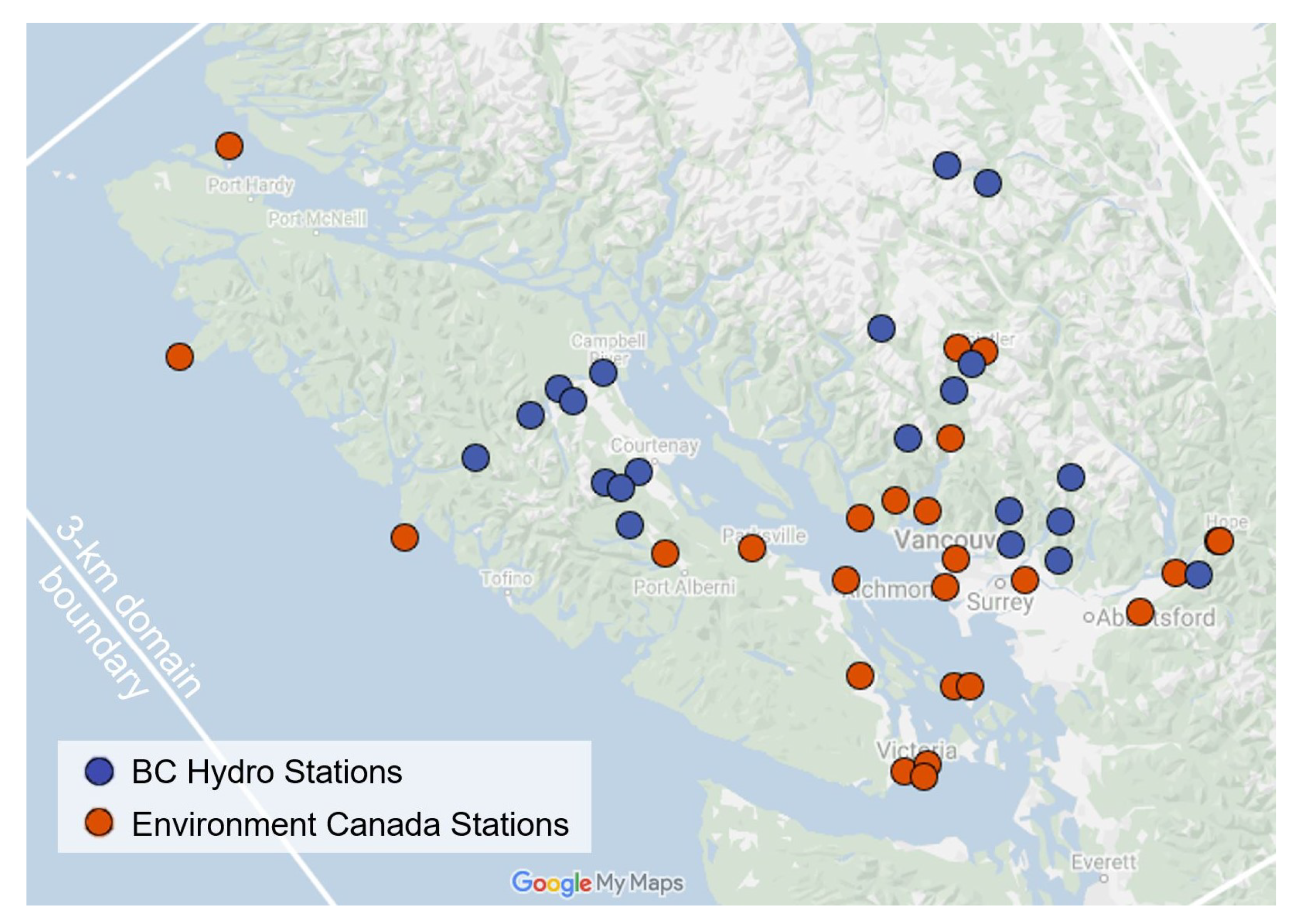
2.1. Data

The NWP data for this study are from the Weather Research and Forecasting (WRF) model [66] version 3.8.1 with the Advanced Research WRF (ARW) dynamical core, initialized with the Global Deterministic Prediction System (GDPS) model [67,68] from Environment and Climate Change Canada (ECCC). The model setup, including initialization, domains, and physics, was chosen based on [58]—a study that evaluated precipitation forecasts from over 100 systematically varied model configurations. We use the WRF configuration from that study that performed above average across verification scores and performed best for 75th-percentile (75p) equitable threat score (ETS) and probability of detection (POD)—namely, the WRF single-moment 5-class microphysics scheme (WSM5; [69]), the Kain-Fritsch cumulus scheme (KF; [70]), the Yonsei University turbulence scheme (YSU; [71]), and the multiphysics Noah land surface model (Noah-MP; [72,73]).
Since [58] found smaller raw forecast errors for coarser grid spacings, but finer grid spacings are assumed to better resolve the spatial variability over complex terrain, this study focuses on the mid-size domain with Δ x = 9-km. WRF runs are initialized daily at 00 UTC and provide 3 days (72 h) of hourly forecast data after 9 h of spinup. Hence, each forecast day starts at 0900 UTC (0100 Local Standard Time). For further details on other WRF settings and the verification results, see [58].
Utilizing this regionally optimized WRF configuration, we generated a 5.75-year reforecast dataset from January 2016 through September 2021. Table 1 lists 22 physical variables that were extracted or derived from the WRF output, some at different vertical levels, resulting in 41 variables total. The list includes general atmospheric parameters that characterize moisture, thermal, stability, and wind conditions. Some variables like MI1 and MI2 were inspired by other precipitation AnEn studies [43,52,54] that used these as predictors.
The model variable “PCP” includes precipitation in all forms (i.e., rainfall, snow, sleet, etc.) and is represented as liquid equivalent. However, BC’s South Coast has a mild climate year-around and freezing temperatures and snowfall are rarely observed at lower elevations.
The original temporal resolution of WRF output is hourly. When assessing longer accumulation windows in this study (i.e., 3-, 6-, 12-hourly, and daily intervals), the sum of hourly PCP is calculated, whereas all other model variables are estimated by their time average. This study considers discrete (non-overlapping) and rolling (overlapping) windows for the accumulated datasets. Discrete-window results are useful for comparison with other studies that use such windows. However, they can split precipitation events unfavorably, making them seem longer and weaker.
Rolling windows, on the other hand, sample the same precipitation events in hourly offsets and ensure the capture of maximum rates for any event and accumulation interval. Therefore they provide a more complete picture in assessing the impact of temporal resolution on predictability. The hourly time step of rolling windows can further benefit temporal trend similarities and supplemental lead times (described below), for which longer-accumulation discrete windows often have too large of a time step. However, it is important to remember that rolling windows possess overlap from one time step to another, which makes them temporally correlated.
46 stations from two networks (ECCC and BC Hydro) provide hourly precipitation observations within the domain of interest, shown in Figure 1. BC Hydro station observations are manually quality controlled at BC Hydro [74]. Additional quality control checks on both observational networks ensure that
  • each station has at least 90% of data available, and missing data is not systematically distributed (e.g., in the same season, at the same time of day, or over a large consecutive period); and
  • outliers are reasonable considering the synoptic situation (e.g., convection), nearby stations, and the available station climatology.
The gridded model data is spatially interpolated to the station locations using the nearest-neighbor approach. The matched station and model dataset is split into 4.75 years (January 2016 through September 2020) for training/optimization using a leave-one-out approach, and one year (the 2021 water year: October 2020 through September 2021) for independent testing/verification. The optimization and verification process both search for analogs from the same 4.75-year training dataset. However, to ensure data independence during optimization, the leave-one-out approach excludes a buffer of ±15 days surrounding the targeted initialization.
Since higher precipitation rates have larger impact and are more challenging to forecast, this study optimizes for performance on “moderate” or heavier precipitation intensities—specifically, 75th percentiles (75p). Section 3.4 provides additional verification results for 90th-percentile (90p) events, i.e., “heavy” precipitation rates. The thresholds are calculated at each station based on observations after excluding values <0.25 mm (which for many rain gauges is the smallest measurable amount). Percentile values vary with accumulation window; examples of frequency distributions are shown in Appendix A.

2.2. Analog Ensemble Methodology

Analog model forecasts (AnFcsts) are a set of past model forecasts (PaFcsts) that, in regard to selected variables and similarity metrics, are most similar to the target model forecast (TaFcst) at a given lead time and location. The past verifying station measurements that correspond to the AnFcsts—the analog observations (AnObs)—are used as ensemble members to compose the AnEn (see Figure 2). The AnEn is considered to be the post-processed version of the deterministic raw TaFcst, and hence should provide a better forecast for the verifying observation (VerifObs) at the target time. Thus, the analog selection is determined solely from the model space, whereas the AnEn is composed solely of samples from the observation space.
Although this study investigates univariate AnEn forecasts for precipitation (i.e., the predictand), a distance measure assesses the multivariate similarity between the TaFcst and all PaFcsts. The best ranking PaFcsts are chosen to be the AnFcsts and are determined independently for each station location and forecast lead time. We use a popular similarity metric developed by [9] that calculates similarity scores
TaFcst t , PaFcsts t = v = 1 N v w v σ v , t j = τ τ ( TaFcst v , t + j PaFcsts v , t + j ) 2 ,
for each PaFcst with the TaFcst at lead-time t relative to model initialization. N v is the number of physical variables v (i.e., predictors) for which closeness between AnFcsts and the TaFcst is desired. The variable weights w v can assign larger importance to variables with stronger predictor relationships. The division by each variable’s standard deviation σ v , t in the model training dataset at lead time t standardizes the variables and makes the similarity scores dimensionless. τ defines a lead-time window that centers the target lead time t and includes additional lead times over which the similarity in the temporal trends of the predictors is computed.
The physical variables that are used for the analog search should exhibit good predictor relationships with the predictand. Precipitation AnEn studies often use model PCP and IWV as predictors [14,16,38] with weights 0.7 and 0.3, respectively, [16,38]. We use these variables as reference when evaluating the predictors that we obtain from other predictor selection techniques (presented in Section 2.2.1). The control run further uses τ = 0, thus only matching the predictor values of TaFcst and PaFcsts at lead time t. The AnEn sensitivity to τ is investigated in Section 3.2. With these reference settings, the optimal AnEn size was found using approximately 30 AnFcst members on average (not shown), which agrees with [33], and is therefore used throughout this study.
To prioritize forecast performance for significant events that are more critical for decision makers, in this study the AnEn parameters are optimized using the 75p threshold-weighted continuous ranked probability score (twCRPS; [7], see Appendix B.1).

2.2.1. Predictor Selection Procedures

The predictor selection procedure objectively assesses which of the 41 model variables in Table 1 are the best predictors for precipitation. Initial investigation of predictor relationships between all variables and observed precipitation using filter methods (e.g., correlation analysis) reveals variability in predictor importance across stations and months (see Appendix C). This is expected since locations and seasons in southwest BC can exhibit different characteristics due to topography and climate. Therefore, we investigate optimal predictors and their weights independently at each station location and meteorological season.
A brute force (BF) approach [35] is a method that runs the AnEn optimization on all combinations of predictor weights (to a defined precision), and determines the best predictor combination according to an evaluation score. Since this method is computationally very expensive, [44] suggested a step-wise forward selection (FS) method, which sequentially selects one predictor at a time by BF testing all weighting options only among the step-wise selected predictors. The first step tests all N v variables as single predictors with w v = 1 (see Equation (1)), and the variable resulting in the best evaluation score is chosen as the first predictor. The next step selects the second predictor by testing the remaining N v 1 variables in combination with the already selected first predictor. The weights applied to each variable are tested by BF, i.e., all possible combinations. For instance, using weight increments of 0.1 in the interval [0, 1] with the constraint that the sum of weights is always 1, results in 9 options for two variables. Selecting the third predictor has ( N v 2 ) 84 , and the fourth predictor has ( N v 3 ) 126 options, etc. Predictors are selected if they improve the evaluation score by a chosen increment compared to the score in the previous FS step (e.g., mean absolute error of 3% in [44]). This way, different stations can receive different numbers of predictors. Although this FS approach is considerably faster than BF, the computational cost is still significant for large N v and high weight precision (i.e., smaller increments).
As a further computational reduction of [44]’s FS, we propose an “efficient FS” (EFS) as follows. Assuming that those variables first selected as predictors have larger importance, we constrain the weighting options to w P r e d i c t o r 1 w P r e d i c t o r 2 . . . w P r e d i c t o r N v . This way the second predictor has ( N v 1 ) 5 , the third predictor has ( N v 2 ) 8 , the third predictor has ( N v 3 ) 9 , and the fourth predictor has only ( N v 4 ) 7 options. We further define the first predictor to be PCP without testing. We proceed to optimize predictors for twCRPS until the improvement drops below 1%.
We investigate four variants of FS to determine predictor weights:
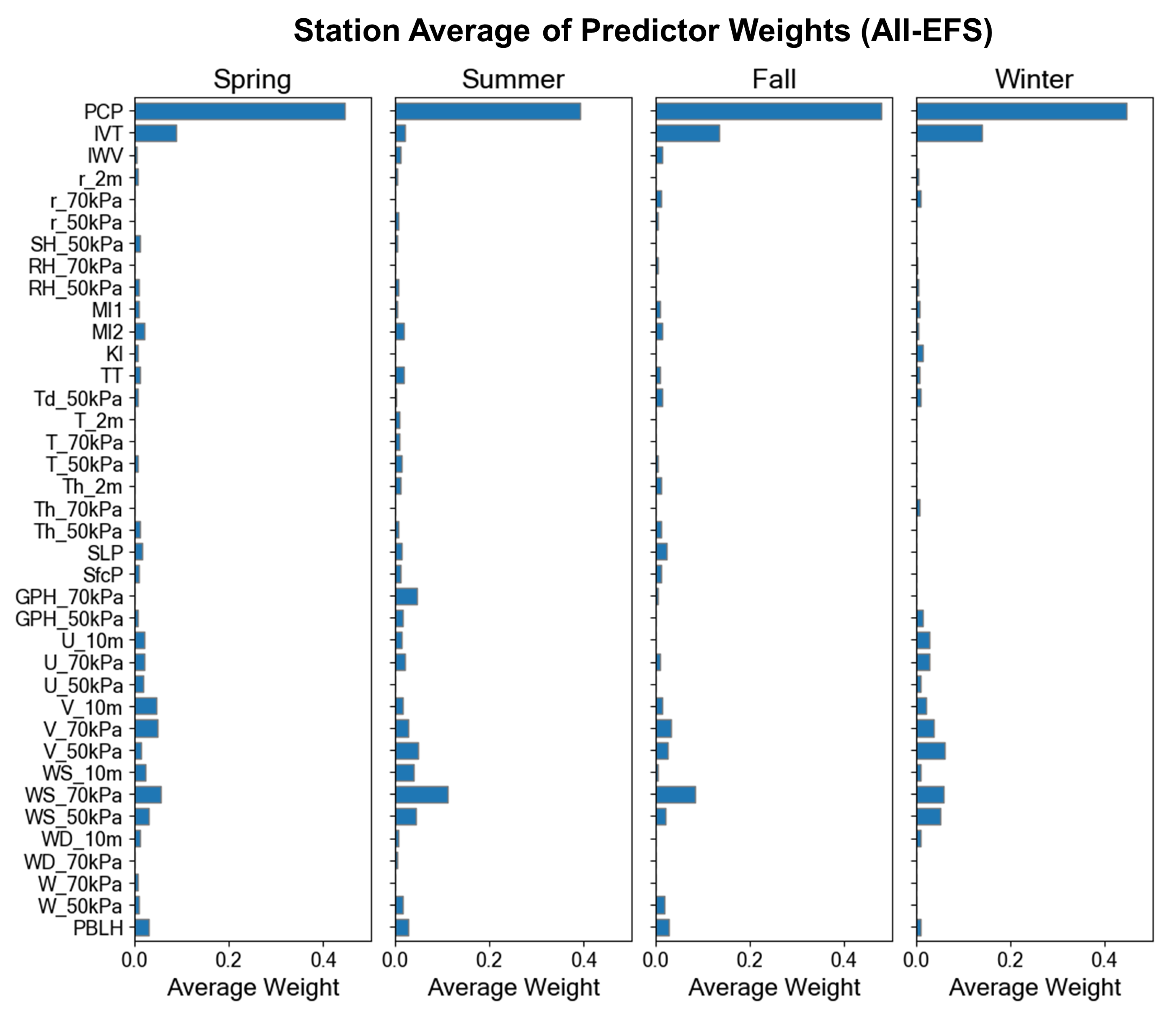
  • All-EFS: Using the EFS to test all 40 variables in addition to PCP as predictors.
  • DC-FS: Using [44]’s FS to test a subset of 10 variables as predictors. The 10 predictor candidates are pre-selected based on the highest distance correlation coefficient (DCorr; a measure that identifies both linear and non-linear relationships [75]) with observed precipitation.
  • DC-EFS: Using the EFS to test the same subset of 10 predictor candidates as in DC-FS.
  • DCV-EFS: Using the EFS to test a subset of 10 variables as predictors, except here, the predictor candidates are based on the best DCorr, as well as the variance inflation factor (VIF, a measure of multicollinearity among variables). Specifically, we grow a set of 10 predictor candidates by sequentially adding one variable at a time, starting from the best ranking DCorr, provided the VIF among the growing set of predictor candidates stays below a threshold value of 10. If this threshold is exceeded it means that the variable exhibits strong correlation with other variables that were already selected and we assume that this variable contributes no additional value as a predictor for the AnEn. Since some of our 41 variables are related (e.g., the same variables at different vertical levels), the VIF check limits the use of correlated and presumably redundant variables in the FS.
These experiments aim to investigate (a) whether the EFS is competitive with [44]’s FS, and (b) whether DCorr or DCorr and VIF can effectively pre-filter meaningful predictor candidates, reducing computational expense compared to testing all variables in EFS. For the feasibility of testing all these methods, we conducted this optimization of predictor weights only for 3-hourly discrete accumulation windows and day-1 forecasts.
We further conducted principal component analysis (PCA) on the standardized datasets of all variables and the 10-variable subsets resulting from DCorr and DCorr-VIF analyses. Different experiments with the principal components (PC) as predictors and their weights either using the eigenvalues or from EFS on the PCs, were not competitive with the (E)FS methods described above and are therefore not shown in this paper. Ref. [35] obtained similar results comparing BF and PCA predictor-selection methods.

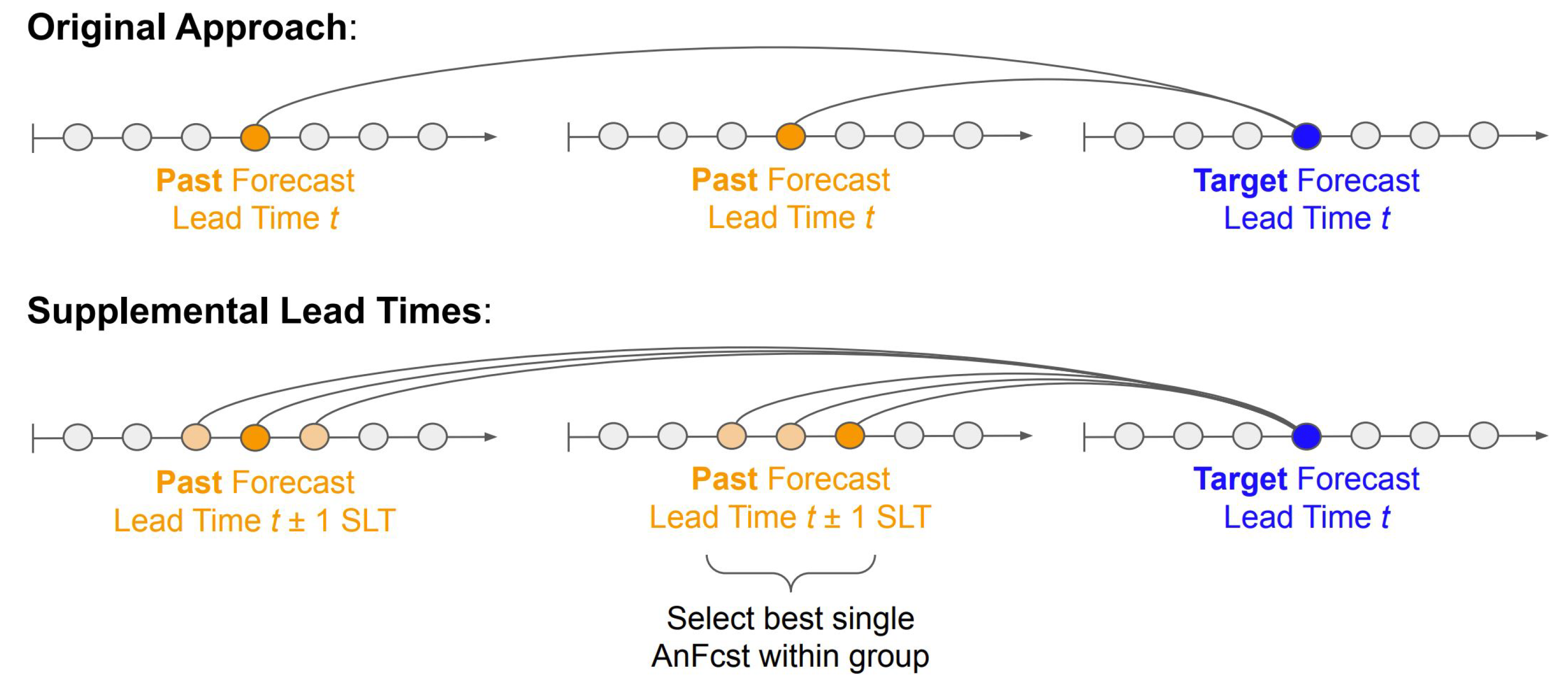
2.2.2. The Supplemental-Lead-Time (SLT) Approach

The original AnEn approach, as described above, searches AnFcsts only across those lead times in the training period that match the target lead time of the TaFcst. The aim of matching lead times is to detect AnFcst candidates with error characteristics similar to the TaFcst. It further ensures that the AnFcsts are sampled from the same time of day, which is particularly important for predictands like temperature and wind that exhibit diurnal cycles. However, precipitation in southwest BC has no significant diurnal cycle in the cool-season when most precipitation occurs; and it is plausible that better AnFcst candidates are available at other lead times surrounding the target lead time, for which model errors are still similar.
Thus, we explore the use of “supplemental lead times” (SLTs) in Section 3.3. As exemplified in Figure 3, AnFcst candidates are considered over a range of offsets from the target lead time. Since AnFcsts from the same past model initialization would be temporally correlated, we only select the best single PaFcst among SLTs from each initialization. Hence, this method selects the AnFcst from a SLT (different from the target lead time) only when the score resulting from Equation (1) indicates closer similarity (i.e., a better analogy).
Accumulation-window treatment must be considered when using SLTs. For instance, ±2 SLTs applied to hourly forecasts selects the best out of five PaFcst options over a lead-time window width of five hours; ±2 SLTs applied to 3-hourly rolling forecasts considers five PaFcst options over a window width of eight hours; and ±2 SLTs applied to 3-hourly discrete forecasts considers five PaFcst options over a total window width of 15 h. Since SLT consideration for longer discrete windows quickly inflates the effective lead-time window width over which model error growth can be significant, we examine SLTs only for short and rolling accumulation windows.
This method differs from [54], who inspected 12-, 6-, and 3-hourly offsets of 24-h accumulations for daily precipitation targets by including all offsets within the 24-h period. For example, [54]’s best-performing 3-hourly offsets result in 8 times as many AnFcst candidates as the original AnEn approach, hereby artificially inflating the meteorological archive with temporally correlated PaFcsts. Our SLT approach, on the other hand, increases the number of AnFcst candidates indirectly by choosing only the single best candidate in the SLT window centering the target lead time, without risking the selection of multiple correlated PaFcsts.

3. Results and Discussion

3.1. Predictor Selection Optimization

The four iterative FS and EFS approaches described in Section 2.2.1 determine predictor weights from the training dataset only. Following optimization for 75p twCRPS, all methods require that the resulting predictors yield better or equal twCRPS compared to the control predictors over the training period. Because the set of 10 predictor candidates used in DC-EFS or DCV-EFS are each a subset of the variables used in All-EFS, it is also required that All-EFS yields better or equal twCRPS during training. It is further required that DC-FS is better than DC-EFS during training, since both methods are preconditioned by the same predictor candidates and the FS approach has more weighting options than EFS. However, running the AnEn over the testing period with the predictor weights determined from the training period reveals whether the selection procedure actually led to the required improvement or whether it overfitted the training dataset.
Figure 4 compares twCRPSS among the four methods, segregated by training and testing. Recall that predictor weights are optimized independently for each station and meteorological season. Therefore, Figure 4 summarizes the twCRPSS of all 46 stations in boxplots and panels for each season.
For all seasons the majority of stations see improvement in twCRPS following predictor optimization with any method. This is true for both training and testing, which indicates that all methods are beneficial. However, the consistent shift between training and testing scores suggests some overfitting; namely, the best predictors during training are still good—but potentially not the best—predictors during testing.
Since summer in BC is by far the driest season, differences in small values of twCRPS between control and optimized predictors are amplified in twCRPSS, hence the larger improvement on average and the large spread. Warm-season dry periods can extend into spring and fall months. The winter season contains the most consistent precipitation pattern.
All methods significantly (see Appendix B.2 for significance testing) improve twCRPS compared to the control during training and testing. However, the differences in twCRPSS among methods are relatively small. Compared to the training, the testing score distributions across stations are less often significantly different among methods. However, winter All-EFS scores are still significantly better than DC-FS and DCV-EFS during testing. Although not always significant, All-EFS is consistently best during training and continues to be best on average (not shown) during testing in summer, fall, and winter. Therefore, we use the predictors resulting from the All-EFS method (see Appendix D) hereinafter. DC-EFS and DCV-EFS are competitive with All-EFS but require considerably less optimization time by assessing only a quarter of the variables. Therefore, they would be viable alternatives for predictor optimization in other studies.
These results show that the EFS approach is capable of effectively reducing the computational effort of predictor tuning compared to [44]’s FS method, while maintaining similar (and sometimes even better) improvements compared to static control predictors.

3.2. Temporal Trend Similarity

In addition to predictor-variable choice and their relative weights, the temporal trends of predictors can also help to better identify AnFcsts. Temporal trend similarity (TTS) is assessed over a time window centered on the target lead time, and window width results from the definition of τ ranging over a number of time steps. The total window width depends on the accumulation window and steps. For instance, a TTS window using ±2 time steps (i.e., τ = 2 in Equation (1)) covers a 5-h period for hourly precipitation, or a 7-h period for 3-hourly rolling windows, whereas it covers an effective 15-h period for 3-hourly discrete windows.
We investigate the impact of TTS with τ ranging from 1 to 5 time steps on twCRPS relative to using no TTS ( τ = 0 ). Since autocorrelation between the predictors and the predictand is unlikely to exceed half a day, for long discrete accumulation windows we discard TTS calculations that would result in effective window widths >36 h. Therefore, 24-hourly discrete windows are not considered for TTS, and 12-hourly discrete windows are assessed only for a TTS with τ = 1 . Note also that there are no forecast values available preceding (following) the first (last) lead time in a forecast series from one initialization; therefore, a few lead times at the beginning and end of a forecast series do not experience the full effect of TTS.
Figure 5 and Figure 6 show that hourly and rolling windows, all of which have hourly time steps, benefit most from TTS. Discrete windows with longer accumulations, and hence larger time steps, cover longer total lead-time widths over which TTS is often less effective—here only on days 2 and 3 is twCRPSS sometimes positive (better) for τ > 0 .
Longer forecast horizons generally obtain better twCRPSS for longer time windows. Due to error growth with lead time, day-1 forecasts exhibit better predictability than day-3 forecasts and thus, day-3 forecasts have greater total potential for improvement. At longer forecast horizons it appears that the added temporal dimension in the similarity consideration somewhat balances the abating quality of the predictor variables, whereas at shorter forecast horizons the instant predictor values preserve higher predictability.
The magnitude of improvement is slightly larger in spring and summer seasons, likely because warm-season precipitation is often convective and has more of a diurnal pattern. However, despite the differences in predictor variables among seasons, the best value of τ is relatively similar across seasons.
Since we determined the optimal values for τ as a function of season, forecast day, and accumulation window, we apply the best significant τ value according to Figure 5 and Figure 6 in the following parts of this study.

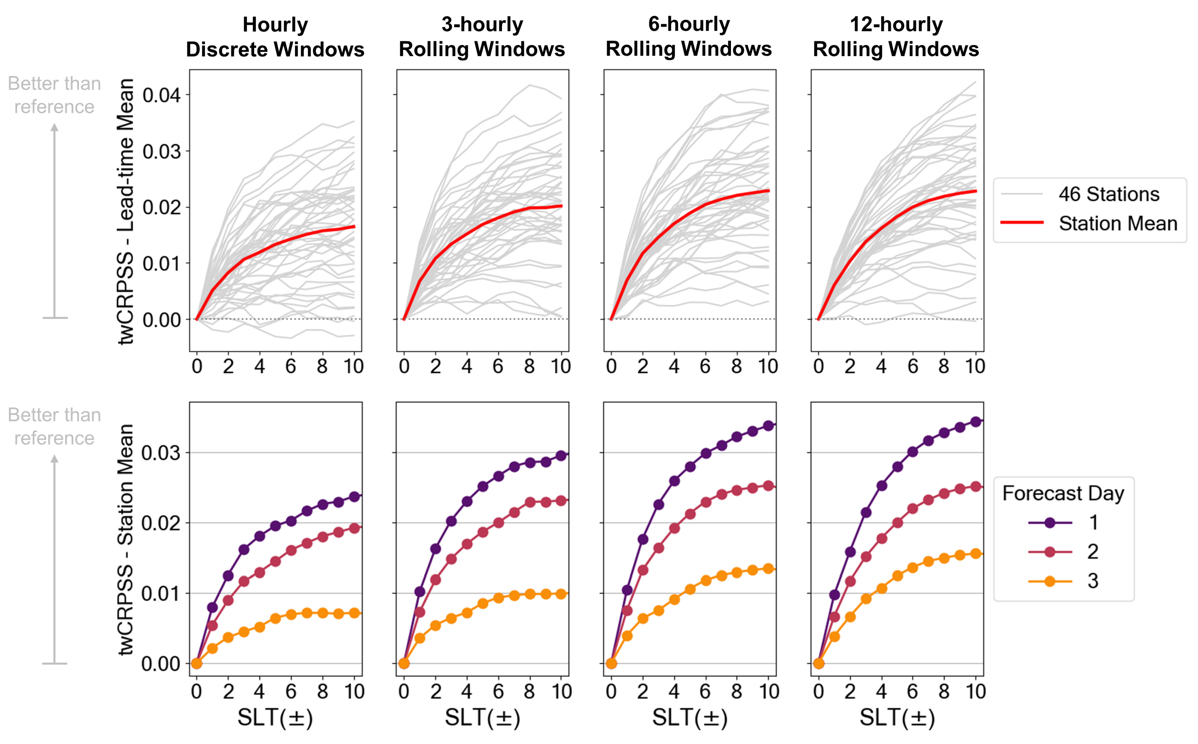
3.3. Supplemental Lead Times (SLTs)
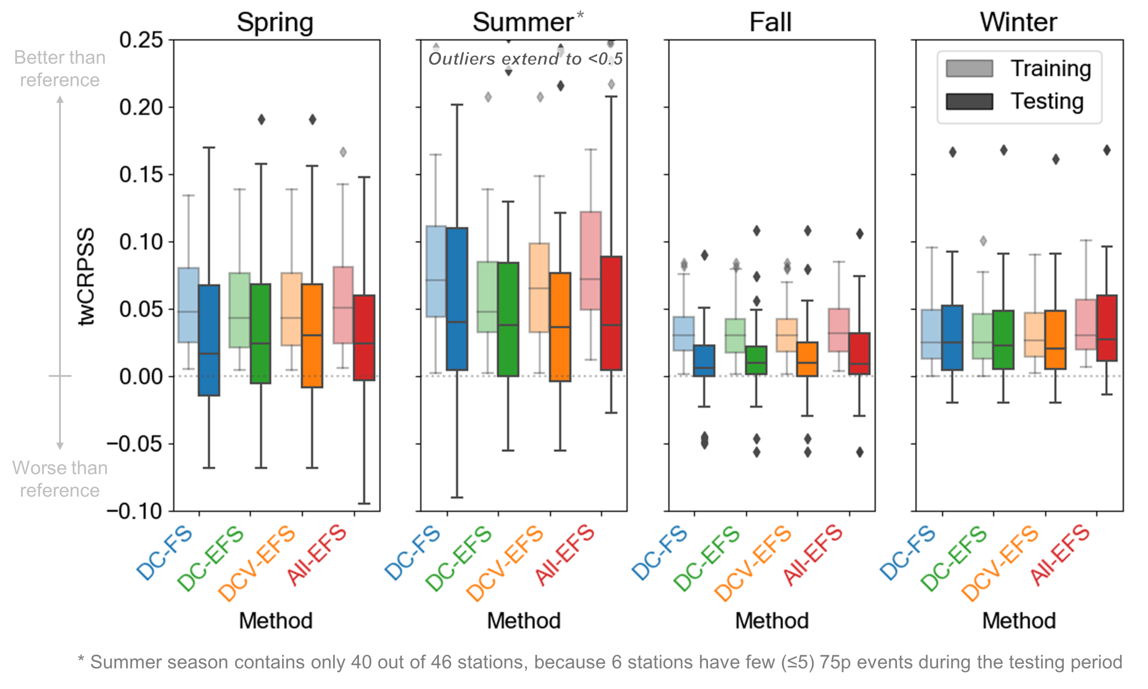
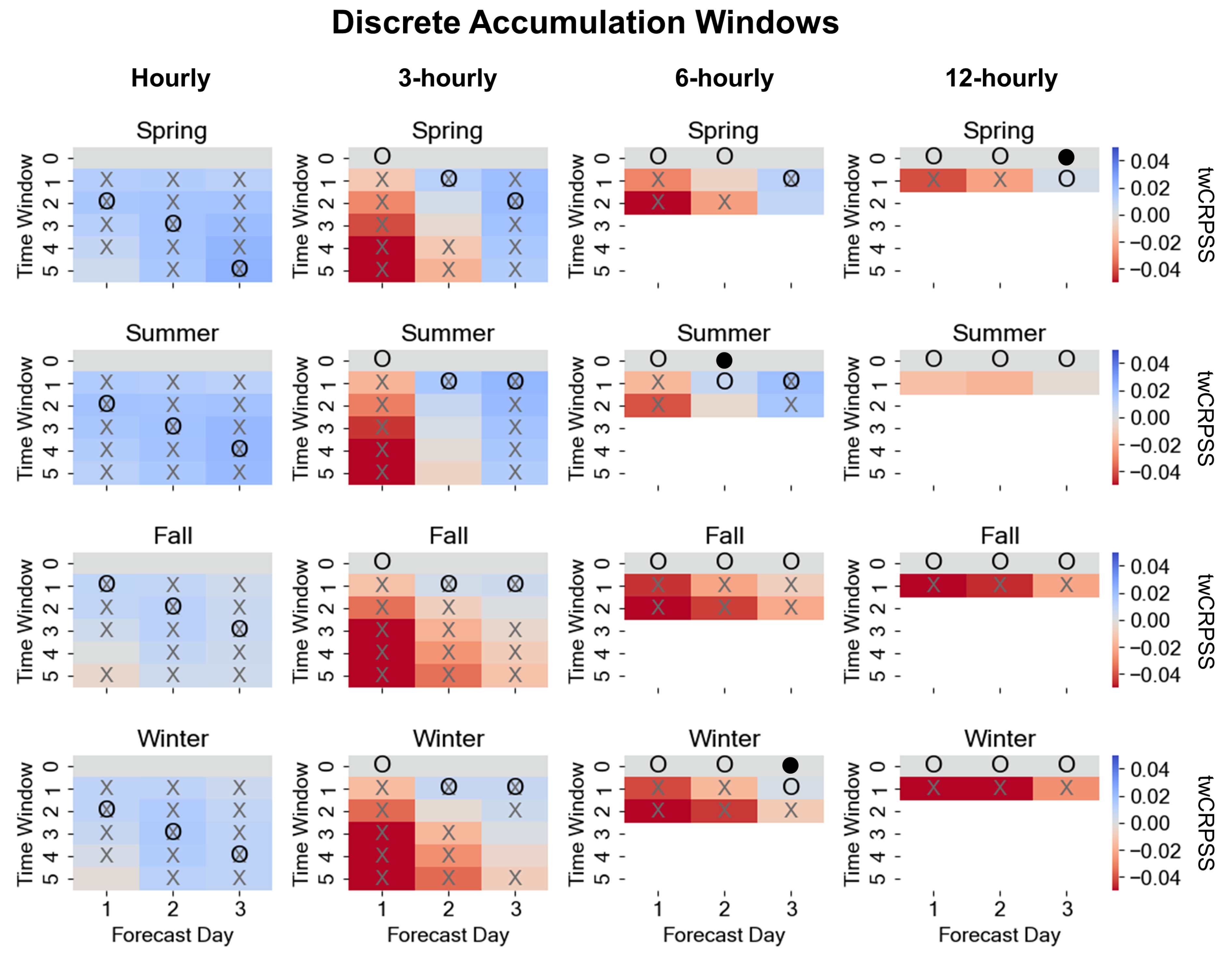
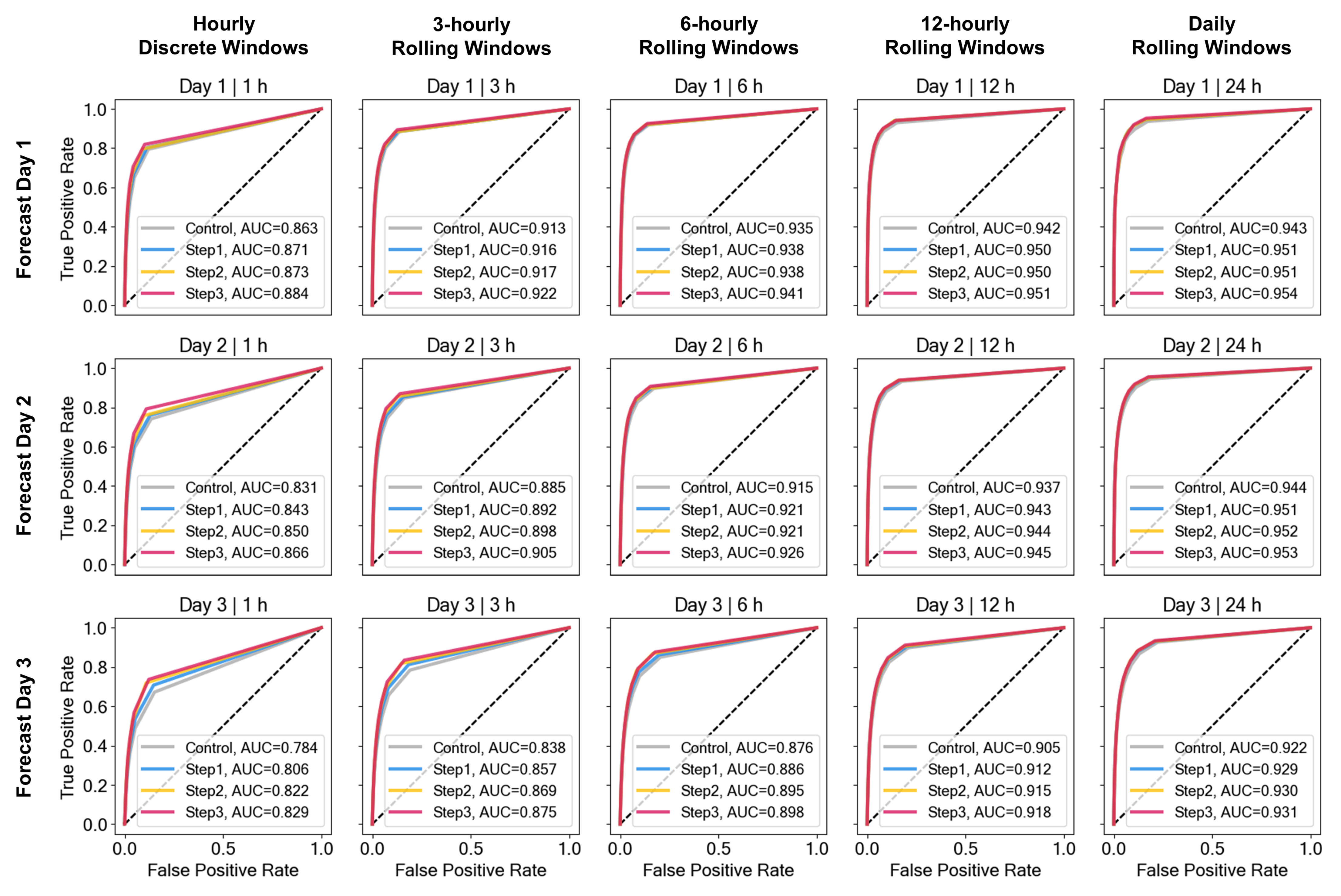
The SLT approach (described in Section 2.2.2) is tested using windows with up to ± 10 SLTs. At this window width the best out of 21 AnFcst candidates is considered, rather than only the one PaFcst at the target lead time as in the original approach. Since we wish to retain error characteristics from similar lead times, we do not assess the effect of SLTs on discrete windows, nor beyond a lead-time offset of 10 h.
Across stations and forecast days, there is a clear tendency that twCRPSS values improve with increasing SLT window (Figure 7). The steepest improvement occurs within ± 3 SLTs and levels out at ± 6 SLTs on forecast day 3, but day-1 and day-2 average scores keep improving at a decreasing rate until our maximum of ± 10 SLTs. Both, twCRPS and twCRPSS changes are significant in every step of growing SLT windows.
While TTS considerations yield best improvements for longer forecast horizons, the SLT approach benefits shorter forecast horizons most. A reason for this could be that on forecast day 1, the limiting factor in AnEn performance is the availability of good analogs from the provided sample size, whereas on day 3, the limiting factor is the quality of the forecast itself.

3.4. Verification

Not all methods could be performed on the discrete accumulations due to their larger time steps, and the predictor selection was in part already evaluated in Section 3.1; therefore, this verification section focuses on hourly and rolling windows only. Verification is conducted by running the AnEn over the independent 1-year testing period with the best tuning parameters determined in Section 3.1, Section 3.2 and Section 3.3. We show the stepwise improvement by comparing:
  • the control AnEn using reference predictors, no TTS, and no SLTs (Control),
  • the AnEn with optimized predictors, but no TTS, and no SLTs (Step 1),
  • the AnEn with optimized predictors and optimized TTS consideration, but no SLT (Step 2), and
  • the AnEn with optimized predictors and optimized TTS consideration, and using SLTs in a window of ± 6 (Step 3).
First, the performance improvement over the raw WRF forecasts is assessed. For comparison we transform the probabilistic AnEn into a deterministic forecast by taking the ensemble median and calculate the mean absolute error (MAE) with the verifying observations. Analogous to Equation (A2) for twCRPSS, the MAE skill score (MAESS) is computed, where positive values represent improvement over the MAE of the raw WRF forecasts.
As seen in Figure 8, all of the AnEn post-processing methods generally have higher rates of improvement for shorter accumulation windows and longer lead times. Even the Control AnEn significantly improves the raw WRF forecasts, and the additional steps further enhance the AnEn performance. For example, the Control AnEn improves WRF MAEs by about 13.3% for hourly forecasts (averaged over forecast days) and about 5.5% for daily forecasts, while the Step 3 AnEn reduces WRF MAEs by an additional 2.9% and 2.0%, respectively. Compared to the Control, our Step 3 AnEn improves hourly-precipitation MAESS by 30.6% on day 1, 26.3% on day 2, and 9.6% on day 3; whereas 12-hourly MAESS are improved by 83.8%, 74.0%, and 41.6%, respectively.
The optimization steps show step-wise improvement, except Step 2 shows a slight drop in MAESS compared to Step 1 for accumulations larger than 3 h. This indicates that the TTS does not always yield the expected improvement as seen during training. The largest improvement is consistently seen in Step 3 from using SLTs.
Recall that the predictor selection was optimized on only forecast day 1 using 3-hourly windows. Yet across accumulation windows and forecast days the same predictors improve the Step 1 MAE, except for daily precipitation on forecast day 1. This study shows results up to daily intervals only for reference, however, users who desire daily-precipitation AnEn forecasts are advised to re-trained the predictor selection to assess whether different variables and weights would make better predictors.
To date, in this paper, we have focused on AnEn improvements for 75p events. Figure 9 and Figure 10 show 90p results to assess if the AnEn forecasts remain skillful for the heavier precipitation events.
The reliability diagrams in Figure 9 show that AnEn probabilities compare well to observed relative frequency across forecast days and accumulation windows; i.e., the AnEns are calibrated and reliable. Relative to the dashed line that represents perfect reliability, most points in the calibration functions have a small deviation towards the left side. This means that the AnEns have a small dry bias for 90p events. This is a common property of AnEns, especially for high-impact events for which only a smaller number of good AnFcsts are available [22,38,48].
Compared to the Control, Step 1 and Step 2 slightly worsen this bias, however, Step 3 moves the calibration function back closer to the line of perfect reliability. This is particularly meaningful because the SLT approach further improves sharpness. Sharper AnEn forecasts were expected as a result of SLTs, because the larger number of considered PaFcsts provides a better chance for the selection of closer AnFcst. These results agree with [54], and they also agree with [38]’s supplemental-locations approach, which uses spatial rather than temporal supplements to inflate the PaFcst sample size.
The receiver operating characteristic (ROC) diagram in Figure 10 shows the discrimination between 90p events and non-events. Larger values of the area under the curve (AUC) score are better, corresponding to a higher true-positive rate (i.e., POD or hit rate) and a lower false-positive rate (i.e., false-alarm rate).
The AnEn AUC scores increase with each optimization step, however, the improvement is larger for shorter accumulations and longer forecast horizons, both of which exhibit worse discrimination to begin with. Although in Figure 8 and Figure 9 Step 2 (TTS) showed smaller improvements or sometimes even worse performance in comparison, TTS contributes considerable improvement with regard to AUC, in particular on forecast day 3 for shorter accumulation windows.

4. Summary and Conclusions

This study demonstrates the benefits of existing and new optimization techniques for AnEn post-processing on sub-daily precipitation forecasts over southwest BC. Lower precipitation rates are easier to predict and have less impact, but since they are far more common they are likely to dominate optimization procedures. Therefore, this study tuned the AnEn parameters for moderate and heavier events based on the 75p twCRPS, instead of the full CRPS as in most other studies.
First, we objectively optimized the choice of predictor variables and their weights by evaluating four variants of forward selection (FS). Since common predictor optimization techniques come at significant computational expense, we suggested the efficient FS (EFS)–an adaptation of [44]’s FS. Limiting the weighting options in sequence with the selected predictors significantly reduces computational cost while maintaining similar optimization performance. Predictor tuning is beneficial even if trained on a portion of the dataset (i.e., only one forecast day instead of the full forecast horizon) and even if the initial set of variables on which the (E)FS is conducted is pre-selected by filter methods such as DCorr. However, EFS on a larger number of meteorological variables can result in minor additional improvements and could be considered in other studies if the computational capacity exists.
Next, we explored the impact of the time-window width over which the temporal predictor trends are matched. This investigation revealed that longer time windows are most beneficial for longer forecast horizons and shorter accumulation windows—a relationship that is often neglected in other studies. Although TTS was shown in the verification Section 3.4 to increase the unconditional dry bias, it improves discrimination of high-impact events. Perhaps the method described in Section 3.2 to assess optimal time windows could be generalized across seasons, such as a staggered implementation for forecast days 1, 2, and 3 using τ equal to 1 or 2, 2 or 3, and 3 or 4, respectively. Caution is advised when using TTS for discrete windows of accumulations that are longer than hourly, because we obtained mixed results dependent on lead time.
Finally, we implemented a new methodology that uses the concept of supplemental lead times (SLTs). It enhances the chance of finding better AnFcsts by allowing the algorithm to choose from forecast lead times within a time window around the target lead time, that should maintain similar error characteristics. This approach is similar to the idea in [54], but it is suitable for shorter accumulations and prevents the selection of temporally dependent AnFcsts. SLTs could be used in addition to [38]’s supplemental locations, or as an alternative if the domain or station sample size is not sufficient (as in this study).
The use of SLTs had the largest impact on AnEn performance, often exceeding the effects of predictor and TTS optimization, especially for verification statistics including the ensemble-median MAE and 90p reliability and sharpness. The time window width for which SLTs showed performance increase is relatively wide in this study, likely because precipitation in BC has no pronounced diurnal cycle in its cool/wet season. Other predictands with more pronounced diurnal cycle would likely require shorter SLT windows and may experience smaller relative improvements. It is conceivable that a longer dataset history would result in similar improvements, dampening the impact of SLTs. However, when relatively short training periods are available (<5 years in this study), the SLT approach somewhat compensates for the small sample size. This opens up opportunities for AnEn applications on shorter but locally optimized and operational data products.
One NWP model forecast produces three-dimensional multivariate deterministic predictions, whereas the AnEn method in this study creates a univariate probabilistic point forecast by post-processing NWP. Compared to NWP ensembles, AnEns are extremely efficient in creating reliable probabilistic point forecasts—that is, if a sufficiently long reforecast dataset is available. Although our algorithm was not optimized for efficiency, a single 3-day forecast at one point location takes on average only 0.5 s to create the Control or Step 1 AnEn on a macOS computer (with 3.2 GHz Intel Core i5 processor), 1 s to create the Step 2 AnEn (with TTS), and <10 s to create the Step 3 AnEn (with TTS and ± 6 SLTs). This computational time applies to the AnFcst search and AnEn composition only (i.e., excluding time for running the NWP TaFcst and interpolation to station locations) and would have to be multiplied by the number of point locations at which forecasts are desired (if not run simultaneously in parallel). In comparison, the three-domain WRF runs used in this study took on average 80 min run time using 48 cores (Intel-compiled WRF code run on an HPC cluster using Open MPI and no hyperthreading on Intel Xeon Processor E5–2683 v4 compute nodes with 2.10 GHz). While at least one NWP run is required to make an AnEn forecast, running an equivalent-sized 30-member WRF ensemble would require 10 runs, which would take approximately 27 core days of run time in serial mode using configurations (e.g., domain setup) as in [58].
In this study, we improved the computational efficiency of AnEn optimization, while also significantly improving AnEn forecast performance by up to 83.8% compared to a reference AnEn. This increase in AnEn performance can be attributed mainly to a new SLT technique. Temporal variability and forecast-error growth cause finer-temporal-resolution and longer-lead-time forecasts to have inherently worse performance, especially over the complex terrain of southwest BC—yet those forecasts benefit the most from the optimized AnEn post-processing. This is an important result in a world where end users desire evermore accurate predictions at finer resolutions and longer outlooks.

Author Contributions

Conceptualization, J.J., G.W. and R.S.; methodology, J.J.; software, J.J.; validation, J.J., G.W. and R.S.; formal analysis, J.J.; investigation, J.J.; resources, R.S. and J.J.; data curation, J.J.; writing—original draft preparation, J.J.; writing—review and editing, G.W. and R.S.; visualization, J.J.; supervision, G.W. and R.S.; project administration, J.J., G.W. and R.S.; funding acquisition, R.S. and G.W. All authors have read and agreed to the published version of the manuscript.

Funding

Computational and storage resources to create the re-forecast dataset and to optimize the AnEns were provided by WestGrid (westgrid.ca) and the Digital Research Alliance of Canada (alliancecan.ca) through the Resource Allocation Competition (RAC) awards 2019–2022. The research was enabled by funding support provided by Mitacs (Grants IT07224 and IT28208), BC Hydro (Contracts 00089063 and 00091424), the Natural Science and Engineering Research Council (NSERC; Discovery Grant RGPIN-2017-03849), and the University of British Columbia (UBC). We thank William Wei Hsieh for supporting this research through the Chih-Chuang and Yien-Ying Wang Hsieh Memorial Scholarship (#5357).

Institutional Review Board Statement

Not applicable.

Informed Consent Statement

Not applicable.

Data Availability Statement

WRF model point forecasts are not publicly archived, but can be reproduced following [58] or made available upon request [contact Roland Stull ([email protected])]. ECCC station data used for verification are available at https://climate.weather.gc.ca/historical_data/search_historic_data_e.html (accessed on 2 November 2021), whereas BC Hydro station data may be obtained by contacting Gregory West ([email protected]).

Acknowledgments

We thank Timothy Chun-Yiu Chui, Yingkai Sha, Henryk Modzelewski, and Roland Schigas for their technical support with this study.

Conflicts of Interest

The authors declare no conflict of interest.

Abbreviations

The following abbreviations are used in this manuscript:
AnEn(s)Analog Ensemble(s)
AnFcst(s)Analog Forecast(s)
AnObsAnalog Observation(s)
TaFcst(s)Target Forecast(s)
VerifObsVerifying Observation(s)
TTSTemporal Trend Similarity
SLT(s)Supplemental Lead Time(s)
FSForward Selection
EFSEfficient Forward Selection

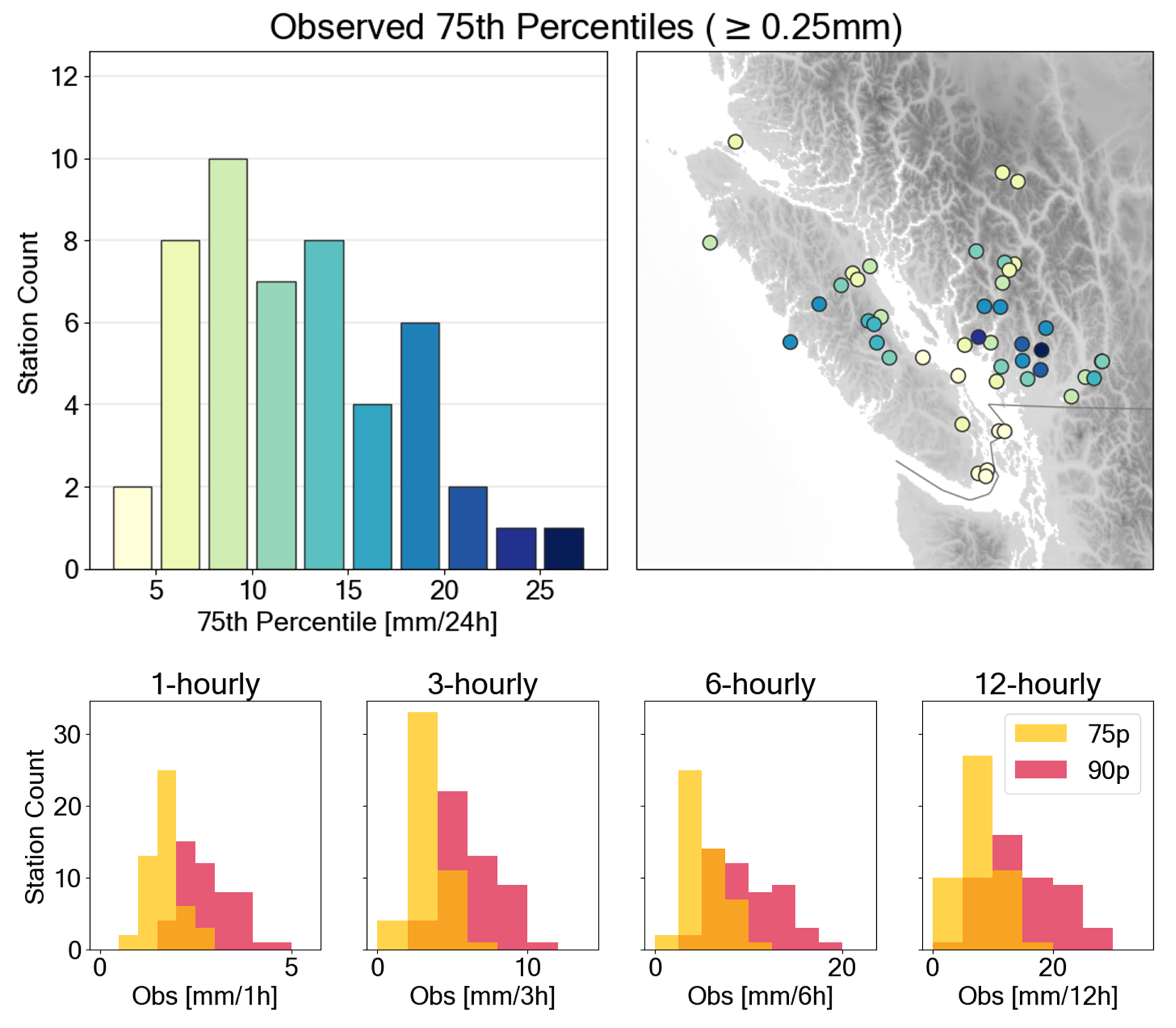
Appendix A. Percentiles

Figure A1. Top row: Histogram of binned daily observed 75th percentiles (75p) at all stations (top left), and corresponding geographic distribution of the 75p relative to topography (top right); Bottom row: Histograms of 75p and 90p for other accumulations. Although not plotted here, these frequency distributions show similar geographic variations to the top right panel.
Atmosphere 13 01662 g0a1

Appendix B. Evaluation

Appendix B.1. Threshold-Weighted Continuous Ranked Probability Score

The 75th-percentile (75p) threshold-weighted continuous ranked probability score [7] across forecasts j is defined as
twCRPS ( AnEn j , VerifObs j ) = 𝟙 { x 75 p } ( AnEn j ( x ) 𝟙 { VerifObs j x } ) 2 d x ,
where 𝟙 denotes an indicator function, which is 1 under the sub-scripted condition, and 0 otherwise, while the conventional CRPS can be interpreted as the integral of the Brier scores over the range of possible thresholds [50,76], the twCRPS with the additional 𝟙 { x 75 p } can be interpreted as the integral of the Brier scores over the thresholds larger than a desired value–75p in our study. In other words, the twCRPS is the fraction of the conventional CRPS that assesses events above the given threshold (the right tail of the distribution).
The relative performance between methods and optimization steps is compared using the threshold-weighted continuous ranked probability skill score
twCRPSS = 1 ( twCRPS ¯ / twCRPS ref ¯ ) ,
which yields positive values when skill is improved compared to the reference.

Appendix B.2. Statistical Tests

If the Shapiro–Wilk test for normality [77] is rejected over the distributions of results across stations, we use the non-parametric two-sided Wilcoxon signed-rank test [78] to assess whether the paired station-result samples from different methods originate from the same distribution at the α = 0.05 level. Otherwise, we use the paired t-test.

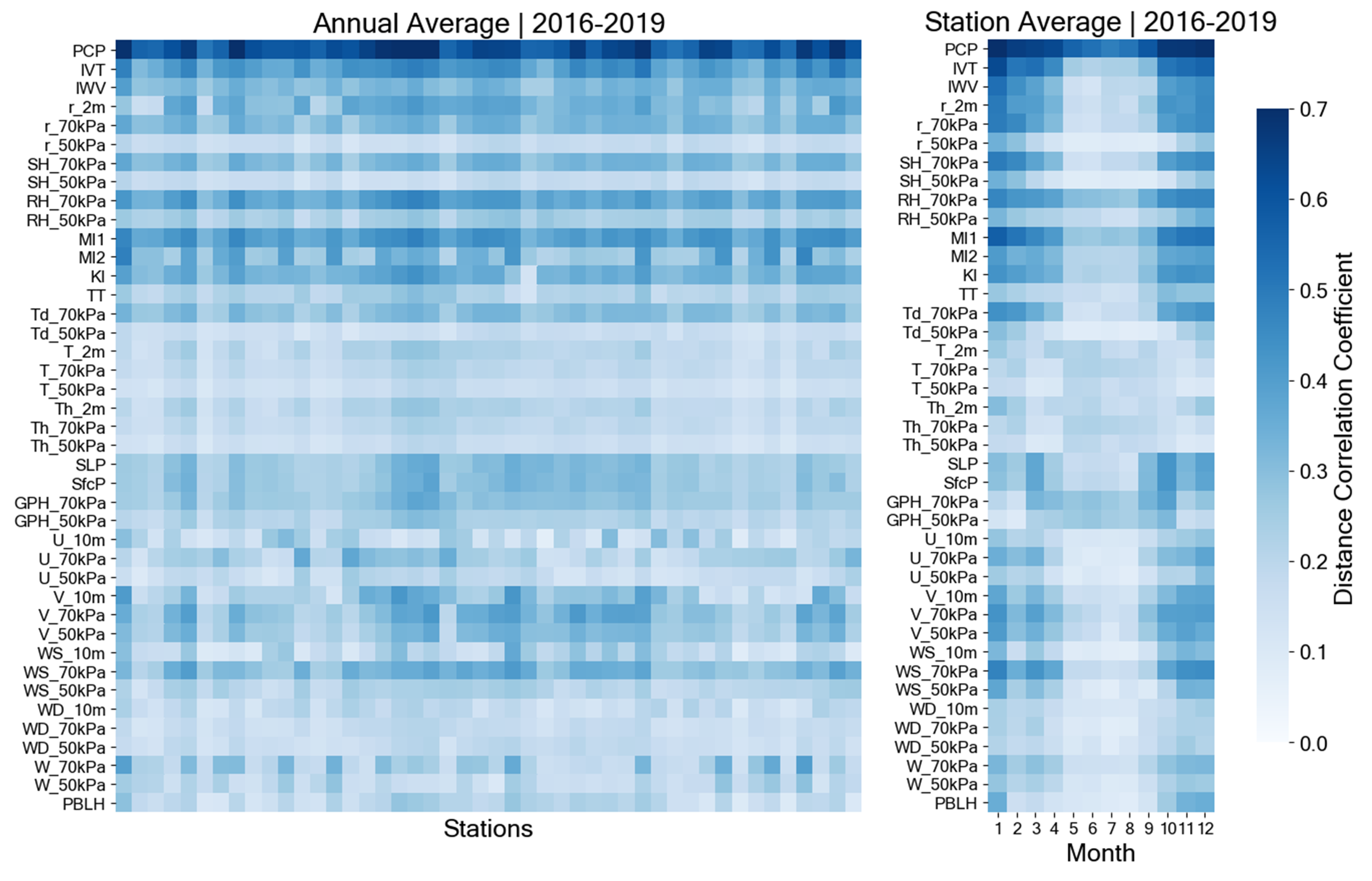
Appendix C. Correlation Analysis

Figure A2. Distance Correlation coefficients (DCorr) of all model variables (see Table 1) with observed precipitation. Variability across 46 stations aggregated over time (left), and variability across months aggregated over stations (right). The time period covers four complete years from the optimization period (rather than the full 4.75-year period) to ensure similar sample size across months.
Atmosphere 13 01662 g0a2

Appendix D. Predictor Weights

Figure A3. Station average of the final predictor weights resulting from the All-EFS method (see Section 2.2.1) for each season. Variables that are in Table 1 but not in the x-axis were never selected by any station at any season.
Atmosphere 13 01662 g0a3

References

  1. Wilks, D.S. Statistical Methods in the Atmospheric Sciences; Elsevier/Academic Press: Cambridge, MA, USA, 2011; p. 676. [Google Scholar]
  2. Wilks, D.S. Extending logistic regression to provide full-probability-distribution MOS forecasts. Meteorol. Appl. 2009, 16, 361–368. [Google Scholar] [CrossRef]
  3. Roulin, E.; Vannitsem, S. Postprocessing of Ensemble Precipitation Predictions with Extended Logistic Regression Based on Hindcasts. Mon. Weather Rev. 2012, 140, 874–888. [Google Scholar] [CrossRef]
  4. Bakker, K.; Whan, K.; Knap, W.; Schmeits, M. Comparison of statistical post-processing methods for probabilistic NWP forecasts of solar radiation. Sol. Energy 2019, 191, 138–150. [Google Scholar] [CrossRef]
  5. Carter, G.M.; Dallavalle, J.P.; Glahn, H.R. Statistical Forecasts Based on the National Meteorological Center’s Numerical Weather Prediction System. Weather Forecast. 1989, 4, 401–412. [Google Scholar] [CrossRef]
  6. Stensrud, D.J.; Yussouf, N. Short-range ensemble predictions of 2-m temperature and dewpoint temperature over New England. Mon. Weather Rev. 2003, 131, 2510–2524. [Google Scholar] [CrossRef]
  7. Gneiting, T.; Ranjan, R. Comparing density forecasts using threshold and quantile-weighted scoring rules. J. Bus. Econ. Stat. 2011, 29, 411–422. [Google Scholar] [CrossRef] [Green Version]
  8. Scheuerer, M. Probabilistic quantitative precipitation forecasting using Ensemble Model Output Statistics. Q. J. R. Meteorol. Soc. 2014, 140, 1086–1096. [Google Scholar] [CrossRef] [Green Version]
  9. Delle Monache, L.; Nipen, T.; Liu, Y.; Roux, G.; Stull, R. Kalman Filter and Analog Schemes to Postprocess Numerical Weather Predictions. Mon. Weather Rev. 2011, 139, 3554–3570. [Google Scholar] [CrossRef] [Green Version]
  10. McCollor, D.; Stull, R. Hydrometeorological accuracy enhancement via postprocessing of numerical weather forecasts in complex terrain. Weather Forecast. 2008, 23, 131–144. [Google Scholar] [CrossRef]
  11. Raftery, A.E.; Gneiting, T.; Balabdaoui, F.; Polakowski, M. Using Bayesian Model Averaging to Calibrate Forecast Ensembles. Mon. Weather Rev. 2005, 133, 1155–1174. [Google Scholar] [CrossRef]
  12. Faidah, D.Y.; Kuswanto, H.; Suhartono. The comparison of Bayesian model averaging with gaussian and gamma components for probabilistic precipitation forecasting. AIP Conf. Proc. 2019, 2192, 090003. [Google Scholar] [CrossRef]
  13. Yuan, H.; Gao, X.; Mullen, S.L.; Sorooshian, S.; Du, J.; Juang, H.M.H. Calibration of Probabilistic Quantitative Precipitation Forecasts with an Artificial Neural Network. Weather Forecast. 2007, 22, 1287–1303. [Google Scholar] [CrossRef]
  14. Sha, Y.; Gagne, D.J., II; West, G.; Stull, R. A hybrid analog-ensemble, convolutional-neural-network method for post-processing precipitation forecasts. Mon. Weather. Rev. 2022, 150, 1495–1515. [Google Scholar] [CrossRef]
  15. Cho, D.; Yoo, C.; Son, B.; Im, J.; Yoon, D.; Cha, D.H. A novel ensemble learning for post-processing of NWP Model’s next-day maximum air temperature forecast in summer using deep learning and statistical approaches. Weather Clim. Extrem. 2022, 35, 100410. [Google Scholar] [CrossRef]
  16. Hamill, T.M.; Whitaker, J.S. Probabilistic Quantitative Precipitation Forecasts Based on Reforecast Analogs: Theory and Application. Mon. Weather Rev. 2006, 134, 3209–3229. [Google Scholar] [CrossRef]
  17. Delle Monache, L.; Eckel, F.A.; Rife, D.L.; Nagarajan, B.; Searight, K. Probabilistic Weather Prediction with an Analog Ensemble. Mon. Weather Rev. 2013, 141, 3498–3516. [Google Scholar] [CrossRef] [Green Version]
  18. Eckel, F.A.; Delle Monache, L. A Hybrid NWP–Analog Ensemble. Mon. Weather Rev. 2016, 144, 897–911. [Google Scholar] [CrossRef]
  19. Junk, C.; Monache, L.D.; Alessandrini, S. Analog-Based Ensemble Model Output Statistics. Mon. Weather Rev. 2015, 143, 2909–2917. [Google Scholar] [CrossRef]
  20. Frediani, M.E.B.; Hopson, T.M.; Hacker, J.P.; Anagnostou, E.N.; Delle Monache, L.; Vandenberghe, F. Object-Based Analog Forecasts for Surface Wind Speed. Mon. Weather Rev. 2017, 145, 5083–5102. [Google Scholar] [CrossRef]
  21. Sperati, S.; Alessandrini, S.; Delle Monache, L. Gridded probabilistic weather forecasts with an analog ensemble. Q. J. R. Meteorol. Soc. 2017, 143, 2874–2885. [Google Scholar] [CrossRef]
  22. Odak Plenković, I.; Delle Monache, L.; Horvath, K.; Hrastinski, M. Deterministic Wind Speed Predictions with Analog-Based Methods over Complex Topography. J. Appl. Meteorol. Climatol. 2018, 57, 2047–2070. [Google Scholar] [CrossRef]
  23. Yang, J.; Astitha, M.; Monache, L.D.; Alessandrini, S. An Analog Technique to Improve Storm Wind Speed Prediction Using a Dual NWP Model Approach. Mon. Weather Rev. 2018, 146, 4057–4077. [Google Scholar] [CrossRef]
  24. Davò, F.; Alessandrini, S.; Sperati, S.; Delle Monache, L.; Airoldi, D.; Vespucci, M.T. Post-processing techniques and principal component analysis for regional wind power and solar irradiance forecasting. Sol. Energy 2016, 134, 327–338. [Google Scholar] [CrossRef] [Green Version]
  25. Alessandrini, S.; Delle Monache, L.; Sperati, S.; Nissen, J. A novel application of an analog ensemble for short-term wind power forecasting. Renew. Energy 2015, 76, 768–781. [Google Scholar] [CrossRef]
  26. Martín, M.; Valero, F.; Pascual, A.; Sanz, J.; Frias, L. Analysis of wind power productions by means of an analog model. Atmos. Res. 2014, 143, 238–249. [Google Scholar] [CrossRef]
  27. Alessandrini, S.; Delle Monache, L.; Sperati, S.; Cervone, G. An analog ensemble for short-term probabilistic solar power forecast. Appl. Energy 2015, 157, 95–110. [Google Scholar] [CrossRef] [Green Version]
  28. Djalalova, I.; Delle Monache, L.; Wilczak, J. PM2.5 analog forecast and Kalman filter post-processing for the Community Multiscale Air Quality (CMAQ) model. Atmos. Environ. 2015, 108, 76–87. [Google Scholar] [CrossRef]
  29. Delle Monache, L.; Alessandrini, S.; Djalalova, I.; Wilczak, J.; Knievel, J.C.; Kumar, R. Improving Air Quality Predictions over the United States with an Analog Ensemble. Weather Forecast. 2020, 35, 2145–2162. [Google Scholar] [CrossRef] [Green Version]
  30. Raman, A.; Arellano, A.F.; Delle Monache, L.; Alessandrini, S.; Kumar, R. Exploring analog-based schemes for aerosol optical depth forecasting with WRF-Chem. Atmos. Environ. 2021, 246, 118134. [Google Scholar] [CrossRef]
  31. Horton, P.; Jaboyedoff, M.; Metzger, R.; Obled, C.; Marty, R. Spatial relationship between the atmospheric circulation and the precipitation measured in the western Swiss Alps by means of the analogue method. Nat. Hazards Earth Syst. Sci. 2012, 12, 777–784. [Google Scholar] [CrossRef]
  32. Ben Daoud, A.; Sauquet, E.; Bontron, G.; Obled, C.; Lang, M. Daily quantitative precipitation forecasts based on the analogue method: Improvements and application to a French large river basin. Atmos. Res. 2016, 169, 147–159. [Google Scholar] [CrossRef] [Green Version]
  33. Keller, J.D.; Monache, L.D.; Alessandrini, S. Statistical Downscaling of a High-Resolution Precipitation Reanalysis Using the Analog Ensemble Method. J. Appl. Meteorol. Climatol. 2017, 56, 2081–2095. [Google Scholar] [CrossRef]
  34. Yang, C.; Yuan, H.; Su, X. Bias correction of ensemble precipitation forecasts in the improvement of summer streamflow prediction skill. J. Hydrol. 2020, 588, 124955. [Google Scholar] [CrossRef]
  35. Junk, C.; Delle Monache, L.; Alessandrini, S.; Cervone, G.; von Bremen, L. Predictor-weighting strategies for probabilistic wind power forecasting with an analog ensemble. Meteorol. Z. 2015, 24, 361–379. [Google Scholar] [CrossRef]
  36. Li, N.; Ran, L.; Jiao, B. An analogy-based method for strong convection forecasts in China using GFS forecast data. Atmos. Ocean. Sci. Lett. 2020, 13, 97–106. [Google Scholar] [CrossRef] [Green Version]
  37. Liu, Y.Y.; Li, L.; Liu, Y.S.; Chan, P.W.; Zhang, W.H.; Zhang, L. Estimation of precipitation induced by tropical cyclones based on machine-learning-enhanced analogue identification of numerical prediction. Meteorol. Appl. 2021, 28, e1978. [Google Scholar] [CrossRef]
  38. Hamill, T.M.; Scheuerer, M.; Bates, G.T. Analog Probabilistic Precipitation Forecasts Using GEFS Reforecasts and Climatology-Calibrated Precipitation Analyses. Mon. Weather Rev. 2015, 143, 3300–3309. [Google Scholar] [CrossRef] [Green Version]
  39. Obled, C.; Bontron, G.; Garçon, R. Quantitative precipitation forecasts: A statistical adaptation of model outputs through an analogues sorting approach. Atmos. Res. 2002, 63, 303–324. [Google Scholar] [CrossRef]
  40. Marty, R.; Zin, I.; Obled, C.; Bontron, G.; Djerboua, A. Toward Real-Time Daily PQPF by an Analog Sorting Approach: Application to Flash-Flood Catchments. J. Appl. Meteorol. Climatol. 2012, 51, 505–520. [Google Scholar] [CrossRef]
  41. Bellier, J.; Zin, I.; Siblot, S.; Bontron, G. Probabilistic flood forecasting on the Rhone River: Evaluation with ensemble and analogue-based precipitation forecasts. E3S Web Conf. 2016, 7, 18011. [Google Scholar] [CrossRef]
  42. Horton, P.; Jaboyedoff, M.; Obled, C. Global Optimization of an Analog Method by Means of Genetic Algorithms. Mon. Weather Rev. 2017, 145, 1275–1294. [Google Scholar] [CrossRef] [Green Version]
  43. Horton, P.; Brönnimann, S. Impact of global atmospheric reanalyses on statistical precipitation downscaling. Clim. Dyn. 2019, 52, 5189–5211. [Google Scholar] [CrossRef]
  44. Alessandrini, S.; Delle Monache, L.; Rozoff, C.M.; Lewis, W.E. Probabilistic Prediction of Tropical Cyclone Intensity with an Analog Ensemble. Mon. Weather Rev. 2018, 146, 1723–1744. [Google Scholar] [CrossRef]
  45. Fernández, J.; Sáenz, J. Improved field reconstruction with the analog method: Searching the CCA space. Clim. Res. 2003, 24, 199–213. [Google Scholar] [CrossRef]
  46. Cannon, A.J. Nonlinear analog predictor analysis: A coupled neural network/analog model for climate downscaling. Neural Netw. 2007, 20, 444–453. [Google Scholar] [CrossRef] [PubMed]
  47. Horton, P.; Jaboyedoff, M.; Obled, C. Using genetic algorithms to optimize the analogue method for precipitation prediction in the Swiss Alps. J. Hydrol. 2018, 556, 1220–1231. [Google Scholar] [CrossRef] [Green Version]
  48. Alessandrini, S.; Sperati, S.; Delle Monache, L. Improving the Analog Ensemble Wind Speed Forecasts for Rare Events. Mon. Weather Rev. 2019, 147, 2677–2692. [Google Scholar] [CrossRef]
  49. Alessandrini, S.; Delle Monache, L.; Rozoff, C.; Lewis, W. Probabilistic Prediction of Hurricane Intensity with an Analog Ensemble. In Proceedings of the 96th American Meteorological Society Annual Meeting, New Orleans, LA, USA, 10–14 January 2016. [Google Scholar]
  50. Odak Plenković, I.; Schicker, I.; Dabernig, M.; Horvath, K.; Keresturi, E. Analog-based post-processing of the ALADIN-LAEF ensemble predictions in complex terrain. Q. J. R. Meteorol. Soc. 2020, 146, 1842–1860. [Google Scholar] [CrossRef] [Green Version]
  51. Hamill, T.M.; Whitaker, J.S.; Mullen, S.L. Reforecasts: An Important Dataset for Improving Weather Predictions. Bull. Am. Meteorol. Soc. 2006, 87, 33–46. [Google Scholar] [CrossRef] [Green Version]
  52. Meech, S.; Alessandrini, S.; Chapman, W.; Delle Monache, L. Post-processing rainfall in a high-resolution simulation of the 1994 Piedmont flood. Bull. Atmos. Sci. Technol. 2020, 1, 373–385. [Google Scholar] [CrossRef]
  53. Dayon, G.; Boé, J.; Martin, E. Transferability in the future climate of a statistical downscaling method for precipitation in France. J. Geophys. Res. Atmos. 2015, 120, 1023–1043. [Google Scholar] [CrossRef]
  54. Horton, P.; Obled, C.; Jaboyedoff, M. The analogue method for precipitation prediction: Finding better analogue situations at a sub-daily time step. Hydrol. Earth Syst. Sci. 2017, 21, 3307–3323. [Google Scholar] [CrossRef] [Green Version]
  55. Gibergans-Báguena, J.; Llasat, M. Improvement of the analog forecasting method by using local thermodynamic data. Application to autumn precipitation in Catalonia. Atmos. Res. 2007, 86, 173–193. [Google Scholar] [CrossRef]
  56. Ren, F.; Ding, C.; Zhang, D.L.; Chen, D.; li Ren, H.; Qiu, W. A Dynamical-Statistical-Analog Ensemble Forecast Model: Theory and an Application to Heavy Rainfall Forecasts of Landfalling Tropical Cyclones. Mon. Weather Rev. 2020, 148, 1503–1517. [Google Scholar] [CrossRef]
  57. Saminathan, S.; Medina, H.; Mitra, S.; Tian, D. Improving short to medium range GEFS precipitation forecast in India. J. Hydrol. 2021, 598, 126431. [Google Scholar] [CrossRef]
  58. Jeworrek, J.; West, G.; Stull, R. WRF Precipitation Performance and Predictability for Systematically Varied Parameterizations over Complex Terrain. Weather Forecast. 2021, 36, 893–913. [Google Scholar] [CrossRef]
  59. Marty, R.; Zin, I.; Obled, C. Sensitivity of hydrological ensemble forecasts to different sources and temporal resolutions of probabilistic quantitative precipitation forecasts: Flash flood case studies in the Cévennes-Vivarais region (Southern France). Hydrol. Process. 2013, 27, 33–44. [Google Scholar] [CrossRef]
  60. Hamill, T.M.; Hagedorn, R.; Whitaker, J.S. Probabilistic forecast calibration using ECMWF and GFS ensemble reforecasts. Part II: Precipitation. Mon. Weather Rev. 2008, 136, 2620–2632. [Google Scholar] [CrossRef] [Green Version]
  61. Fernández-Ferrero, A.; Sáenz, J.; Ibarra-Berastegi, G. Comparison of the performance of different analog-based bayesian probabilistic precipitation forecasts over Bilbao, Spain. Mon. Weather Rev. 2010, 138, 3107–3119. [Google Scholar] [CrossRef]
  62. Chapman, W.E.; Delle Monache, L.; Alessandrini, S.; Subramanian, A.C.; Ralph, F.M.; Xie, S.P.; Lerch, S.; Hayatbini, N. Probabilistic Predictions from Deterministic Atmospheric River Forecasts with Deep Learning. Mon. Weather Rev. 2021, 150, 215–234. [Google Scholar] [CrossRef]
  63. PCIC. Atmospheric Rivers State of Knowledge Report; Technical Report; Pacific Climate Impacts Consortium: Victoria, BC, Canada, 2013; Available online: https://www.pacificclimate.org/sites/default/files/publications/Atmospheric%20Report%20Final%20Revised.pdf (accessed on 2 November 2021).
  64. Gillett, N.P.; Cannon, A.J.; Malinina, E.; Schnorbus, M.; Anslow, F.; Sun, Q.; Kirchmeier-Young, M.; Zwiers, F.; Seiler, C.; Zhang, X.; et al. Human influence on the 2021 British Columbia floods. Weather Clim. Extrem. 2022, 36, 100441. [Google Scholar] [CrossRef]
  65. Vasquez, T. How an Atmopsheric River Flooded British Columbia. Weatherwise 2022, 75, 19–23. [Google Scholar] [CrossRef]
  66. Skamarock, W.; Klemp, J.; Dudhi, J.; Gill, D.; Barker, D.; Duda, M.; Huang, X.Y.; Wang, W.; Powers, J. A Description of the Advanced Research WRF Version 3; Technical Report; University Corporation for Atmospheric Research: Boulder, CO, USA, 2008. [Google Scholar] [CrossRef]
  67. Côté, J.; Gravel, S.; Méthot, A.; Patoine, A.; Roch, M.; Staniforth, A. The Operational CMC–MRB Global Environmental Multiscale (GEM) Model. Part I: Design Considerations and Formulation. Mon. Weather Rev. 1998, 126, 1373–1395. [Google Scholar] [CrossRef]
  68. Girard, C.; Plante, A.; Desgagné, M.; McTaggart-Cowan, R.; Côté, J.; Charron, M.; Gravel, S.; Lee, V.; Patoine, A.; Qaddouri, A.; et al. Staggered Vertical Discretization of the Canadian Environmental Multiscale (GEM) Model Using a Coordinate of the Log-Hydrostatic-Pressure Type. Mon. Weather Rev. 2014, 142, 1183–1196. [Google Scholar] [CrossRef]
  69. Hong, S.Y.; Dudhia, J.; Chen, S.H. A Revised Approach to Ice Microphysical Processes for the Bulk Parameterization of Clouds and Precipitation. Mon. Weather Rev. 2004, 132, 103–120. [Google Scholar] [CrossRef]
  70. Kain, J.S. The Kain–Fritsch Convective Parameterization: An Update. J. Appl. Meteorol. 2004, 43, 170–181. [Google Scholar] [CrossRef]
  71. Hong, S.Y.; Noh, Y.; Dudhia, J. A New Vertical Diffusion Package with an Explicit Treatment of Entrainment Processes. Mon. Weather Rev. 2006, 134, 2318–2341. [Google Scholar] [CrossRef] [Green Version]
  72. Niu, G.Y.; Yang, Z.L.; Mitchell, K.E.; Chen, F.; Ek, M.B.; Barlage, M.; Kumar, A.; Manning, K.; Niyogi, D.; Rosero, E.; et al. The community Noah land surface model with multiparameterization options (Noah-MP): 1. Model description and evaluation with local-scale measurements. J. Geophys. Res. Atmos. 2011, 116, 1–19. [Google Scholar] [CrossRef] [Green Version]
  73. Yang, Z.L.; Niu, G.Y.; Mitchell, K.E.; Chen, F.; Ek, M.B.; Barlage, M.; Longuevergne, L.; Manning, K.; Niyogi, D.; Tewari, M.; et al. The community Noah land surface model with multiparameterization options (Noah-MP): 2. Evaluation over global river basins. J. Geophys. Res. Atmos. 2011, 116. [Google Scholar] [CrossRef]
  74. Sha, Y.; Gagne, D.J., II; West, G.; Stull, R. Deep-Learning-Based Precipitation Observation Quality Control. J. Atmos. Ocean. Technol. 2021, 38, 1075–1091. [Google Scholar] [CrossRef]
  75. Székely, G.J.; Rizzo, M.L.; Bakirov, N.K. Measuring and testing dependence by correlation of distances. Ann. Stat. 2007, 35, 2769–2794. [Google Scholar] [CrossRef]
  76. Smith, L.A.; Suckling, E.B.; Thompson, E.L.; Maynard, T.; Du, H. Towards improving the framework for probabilistic forecast evaluation. Clim. Chang. 2015, 132, 31–45. [Google Scholar] [CrossRef] [Green Version]
  77. Shapiro, S.S.; Wilk, M.B. An Analysis of Variance Test for Normality (Complete Samples). Biometrika 1965, 52, 591–611. [Google Scholar] [CrossRef]
  78. Wilcoxon, F. Individual Comparisons by Ranking Methods. Biom. Bull. 1945, 1, 80–83. [Google Scholar] [CrossRef]
Figure 1. Domain of interest in southwest British Columbia with locations of 46 stations that provide hourly precipitation observations from two networks.
Atmosphere 13 01662 g001
Figure 2. Illustration of the analog ensemble (AnEn) methodology.
Atmosphere 13 01662 g002
Figure 3. Graphic of the supplemental-lead-time approach (SLT; bottom), compared to the original approach (top). The circles along the arrows represent lead times of an initialization. This example illustrates the analog search at lead time t. For the first past-forecast (PaFcst) initialization, the SLT approach using ±1 SLTs selects the analog forecast (AnFcst) at lead time t as in the original approach. For the second PaFcst initialization, the SLT approach finds a better AnFcst at lead time t + 1 .
Atmosphere 13 01662 g003
Figure 4. Box-and-whisker plots of 75p twCRPSS distributions across stations (46 stations in each boxplot, except in summer) after predictor optimization with four methods. The dotted zero line separates values that indicate improvement (positive values) vs. deterioration (negative values) compared to the reference twCRPS using control predictors. Performance differences between training (lighter colors) and testing (darker colors) informs about the degree of overfitting.
Atmosphere 13 01662 g004
Figure 5. Heatmaps of station-averaged twCRPSS for hourly to 12-hourly discrete accumulation windows using τ between 1 and 5 to consider temporal trend similarity (TTS) for all seasons and forecast windows. Blue (red) colors indicate better (worse) average twCRPS compared to the reference using τ = 0 (no TTS). Crosses “X” mark significant differences in twCRPS station distributions compared to the reference. Empty circles mark the value τ that exhibits best improvement overall, and filled circles correct the position of best τ if the value in the empty circle is not significant.
Atmosphere 13 01662 g005
Figure 6. As in Figure 5 but for 3-hourly to daily rolling windows. Again, empty circles mark the value τ that exhibits best improvement overall, and filled circles correct the position of best τ if the value in the empty circle is not significant. Forecast day 1 for daily accumulations is removed, since it contains only 1 instead of 24 lead-time samples as on the other forecast days.
Atmosphere 13 01662 g006
Figure 7. Lead-time aggregated (top) and station-aggregated (bottom) twCRPSS from the supplemental-lead-time (SLT) experiments. The reference for twCRPSS is the original approach with optimized predictors but without SLT. Positive twCRPSS indicate improvement compared to the reference.
Atmosphere 13 01662 g007
Figure 8. Station mean of the mean absolute error skill score (MAESS) by forecast day and for hourly to daily rolling windows, relative to the raw NWP forecast.
Atmosphere 13 01662 g008
Figure 9. Station-aggregated 90p reliability diagrams on all forecast days for hourly discrete to daily rolling accumulation windows. The dashed black line is the reference for perfect reliability, the grey dotted lines show climatological probability. The inset in the lower right corner displays the corresponding sharpness diagram, which shows the relative frequency of forecasts that fall into each bin. Due to the skewed nature of precipitation distributions, the y-axis in the sharpness diagram is plotted on a logarithmic scale. The reliability diagram displays only bins that include at least 50 samples in total (i.e., only those points above the dashed grey line in the sharpness diagram).
Atmosphere 13 01662 g009
Figure 10. Station-aggregated 90p receiver operating characteristic (ROC) diagrams for all forecast days and hourly discrete to daily rolling accumulation windows. The area under the curve (AUC) is given in each legend and has a perfect score of 1. The dashed black line represents the line of no skill with AUC = 0.5 corresponding to climatology.
Atmosphere 13 01662 g010
Table 1. Physical variables extracted from the WRF model output and considered as predictors.
VariableAbbreviationLevels
Total PrecipitationPCPSurface
Integrated Water Vapor *IWVColumn
Integrated Vapor Transport *IVTColumn
Water Vapor Mixing Ratior2 m, 70 kPa, 50 kPa
Specific Humidity *SH70 kPa, 50 kPa
Relative Humidity *RH70 kPa, 50 kPa
Moisture Index 1 * ( R H 70 k P a × I W V )MI1
Moisture Index 2 * ( R H 70 k P a × W 70 k P a )MI2
TemperatureT2 m, 70 kPa, 50 kPa
Potential TemperatureTh2 m, 70 kPa, 50 kPa
Dewpoint TemperatureTd70 kPa, 50 kPa
Total Totals Index *TT
K-Index *KI
U-component WindU10 m, 70 kPa, 50 kPa
V-component WindV10 m, 70 kPa, 50 kPa
W-component WindW70 kPa, 50 kPa
Wind Direction *WD10 m, 70 kPa, 50 kPa
Wind Speed *WS10 m, 70 kPa, 50 kPa
Sea Level PressureSLPSea Level
Surface PressureSfcPSurface
Geopotential HeightGPH70 kPa, 50 kPa
Boundary Layer HeightPBLH
* Derived from WRF output variables.
Publisher’s Note: MDPI stays neutral with regard to jurisdictional claims in published maps and institutional affiliations.

