Abstract
Nowcasting of clouds is a challenging spatiotemporal task due to the dynamic nature of the atmosphere. In this study, the use of convolutional gated recurrent unit networks (ConvGRUs) to produce short-term cloudiness forecasts for the next 3 h over Europe is proposed, along with an optimisation criterion able to preserve image structure across the predicted sequences. This approach is compared against state-of-the-art optical flow algorithms using over two and a half years of observations from the Spinning Enhanced Visible and Infrared Imager (SEVIRI) instrument onboard the Meteosat Second Generation satellite. We show that the ConvGRU trained using our structure-preserving loss function significantly outperforms the optical flow algorithms with an average change in , mean absolute error and structural similarity of 12.43%, −8.75% and 9.68%, respectively, across all time steps. We also confirm that merging multiple optical flow algorithms into an ensemble yields significant short-term performance increases (<1 h), and that nowcast skill can vary significantly across different European regions. Furthermore, our results show that blurry images resulting from using globally oriented loss functions can be avoided by optimising for structural similarity when producing nowcasts. We thus showcase that deep-learning-based models using locally oriented loss functions present a powerful new way to produce accurate cloud nowcasts, with important applications to be found in solar power forecasting.
1. Introduction
Accurately modelling the evolution of clouds remains one of the greatest uncertainties in modern climate models today [1]. Clouds play a central role in the solar irradiation balance of the earth, being responsible for a net cloud radiative forcing effect of −20 W/m2 at the top of our atmosphere [2], and thus are major drivers of global hydrological and energy cycles. Being able to accurately predict cloud evolution in the short term will aid forecast potentially hazardous events such as severe convective weather, precipitation, and enable better operational planning for solar photovoltaic power plants. Nowcasting lends itself well to the short-term prediction of cloudiness, as its focus is on forecasting how the atmosphere will evolve within a time frame of 0 up to 6 h as defined by the World Meteorological Organisation [3].
Nowcasting methods have been employed since the 1970s to predict convective initiation from radar data and satellite imagery [4], as these types of mesoscale phenomena have often been linked to high precipitation rates and thunderstorm development, and are thus of great importance to society. Current mesoscale nowcasting methods often rely on multispectral satellite data for cloud nowcasting. This firstly involves determining what pixels inside of a scene represent clouds, resulting in the creation of a cloud mask layer [5]. Such cloud masks are computed from a combination of visible and infrared data from orbiting geostationary satellites [6] and can be further processed to classify clouds into their respective cloud types, such as low-level liquid water clouds or high-altitude ice clouds which can be identified through their different cloud optical properties.
Currently, the most well established technique to nowcast cloud evolution is the computation of cloud motion vectors (CMV) using optical flow (OF) methods such as the Lucas–Kanade algorithm [7,8]. This pixel-based methodology calculates a motion vector field from two or more consecutive images, with the resulting motion vector field being used to warp the last image into the direction of computed pixel motion, with the resulting image being the forecast. This optical flow method is particularly widespread for operational precipitation nowcasting systems such as the Hong Kong Observatory’s SWIRLS system or the UK Met Office’s STEPS system [9,10]. Increasingly, optical flow methods have also been applied in the cloud nowcasting domain, specifically for the purpose of forecasting solar radiation at photovoltaic power plants, which is one of the main motivations of this study [11].
However, a potential pitfall of the optical flow approach is that it can only predict the movement of features currently found within a given image and does not take into account longer-term time dependencies between multiple consecutive observations within the data. Furthermore, other physical processes leading to cloud formation such as orographic lifting, convergence and frontal lifting may not be adequately captured by this method. With today’s advances in communication protocols, computing power and a vast increase in remote sensing data, cloud nowcasting approaches have now been able to diversify greatly beyond the CMV estimation approach. Other methods have included enhancing CMVs with voxel-carving-based approaches [12], which enable tracking individual clouds in voxel space, and the creation of a subsequent irradiance map to be used for solar radiation nowcasting. More traditional time series forecasting methods such as autoregressive integrated moving average (ARIMA) models [13] have also been used for solar radiation nowcasting, using an on-site pyranometer to measure changes in the direct normal irradiance (DNI) at the site, which is directly affected by passing clouds.
Some of the most recent approaches to nowcasting solar radiation and clouds make use of deep neural networks (DNNs) and data collected by all sky imagers at photovoltaic power plants [14]. For example, a range of attention-based convolutional neural networks (CNN) were trained on historical photovoltaic power values and sky images to estimate photovoltaic power. However, these approaches are limited to covering a small geographic area and are not able to extrapolate to larger areas as would be possible with the usage of satellite data making these methods limited and expensive to roll out across a larger operational nowcasting context. In contrast, using high-resolution satellite data enables the covering of a large nowcasting extent in an efficient manner, with multiple years of available historical observations providing a large amount of information for a deep learning model to learn how to represent short-term cloud dynamics.
To take advantage of this growing quantity of data, deep-learning-based models present novel and efficient ways of learning patterns in historical atmospheric observations. In particular it has been shown that model architectures which combine autoencoders with recurrent units outperform state-of-the-art optical flow algorithms in precipitation nowcasting, which like cloud nowcasting, aims at forecasting the future positions of moving objects, whilst considering time series of images as both inputs and targets of the model in consideration [15,16,17,18,19,20]. Autoencoder architectures enable a model to learn a compressed representation of an input (for example a sequence of cloud fields), whilst recurrent units such as long short-term memory (LSTM) or gated-recurrent units (GRU) capture the complex dynamics within the temporal ordering of input sequences. Furthermore, they enable models once trained to work with a variable length of input sequences and thus make for a flexible nowcasting system.
Thus, the goal of this study was to apply recent advances in the nowcasting of precipitation to the cloud nowcasting task, whilst validating our approach across large portions of Western Europe and improving on the shortcomings found in recent cloud nowcasting studies. To our best knowledge, cloud nowcasting using deep learning has so far only been explored by a small number of studies, and within a limited spatial and temporal scope. Knol et al. trained a convolutional autoencoder network using 486 days of EUMETSAT normalised irradiance data from the Netherlands and evaluated their model on 75 days of unseen test data. Although they showed that their model outperformed optical flow forecasts on average by 8% in mean absolute error (MAE) they reported that their generated forecasts rapidly degraded in structural quality and became blurry [21]. Furthermore, Berthomier et al. showed that deep-learning-based models (U-Net, CNN) were able to outperform the AROME numerical weather prediction model for cloud cover predictions over France in terms of mean squared error (MSE), but also reported that predictions by their model produced blurry edges [20]. Similar findings highlighting blurred forecasts by deep learning models were also reported by Ioenscu et al. who nowcasted a series of EUMETSAT satellite products over Southeast Europe [22] as well as Yang and Mehrkanoon [23], who proposed that one of the reasons for the blurring may be due to the use of MSE as the objective function for training the models, which all other mentioned studies with blurry forecasts also used as their loss function.
In light of these recent findings, we propose a solution to the blurry image problem encountered in previous cloud nowcasting research, by developing a deep-learning-based cloud nowcasting model which is optimised to preserve the structural integrity of its nowcasts. This is important as for operational nowcasting, blurry predictions reduce the spatial accuracy of the forecasts, which is an important forecast attribute to retain, especially for applications in the solar energy industry. To achieve this, we develop a convolutional autoencoder model which is optimised using a combination of locally and globally oriented loss functions, which optimise for structural similarity between the input and target cloud sequences, and we compare its nowcasting performance to state-of-the-art optical flow models to produce blur-free nowcasts. We validate our approach across a large portion of Western Europe, and set our nowcasting lead times to 3 h, enabling our nowcasting models to be deployed as part of short-term forecasting systems, as we envision this system to operate in a blended context, with longer timescale predictions from 3 to 6 h being handled by a numerical weather prediction model such as the Icosahedral Nonhydrostatic Weather and Climate Model (ICON).
2. Materials and Methods
Data Source
The primary dataset for this study consisted of over two and a half years of daily outputs from the Meteosat Second Generation Cloud Physical Properties (MSG-CPP) algorithm (1 January 2018–18 October 2020) developed at the Royal Netherlands Meteorological Institute (KNMI) [6]. This dataset provides derived cloud and radiation products from the Spinning Enhanced Visible and Infrared Imager (SEVIRI) instrument onboard the Meteosat Second Generation satellite operated by EUMETSAT with a resolution of 3 × 3 km2. In particular, 1022 days of data with a temporal availability of 15 min were gathered in total, constituting approximately 560 GB of raw data.
Specifically, shortwave down-welling direct radiation was extracted from this dataset, which was derived from methods described by Greuell et al. [24], which provide a physics-based algorithm providing direct radiation and clear sky radiation products. All radiative transfer calculations were parametrised by the surface albedo, integrated water vapour and cosine of the solar zenith angle, while cloud parameters included cloud optical thickness as well as effective droplet radius (for water clouds) and effective crystal radius (for ice clouds). Direct normal radiation assuming clear sky incorporated the aerosol optical thickness at 500 nm, the Ångström exponent, aerosol single-scattering albedo as well as the surface elevation. Thus, we produced a proxy field of cloudiness (representing water and ice clouds), with values between 0 and 1, by computing the fraction of shortwave down-welling direction radiation divided by the direct solar radiation assuming clear sky, with this variable forming the primary sequence variable to nowcast in this study (see Figure A1 for an example training sequence).
In order to produce geographically accurate cloud forecasts, the raw MSG-CPP satellite imagery had to be reprojected from a geostationary satellite grid to a map projection corresponding to the area of interest. Furthermore, as the nowcasting methods in this study employed displacement-vector-based calculations and convolutions when computing pixel displacement, the transverse Mercator projection was selected, as it preserves angles to an infinitesimal scale and has low distortion near the central meridian. After reprojection, a total of 9 different spatial extents covering 16 different countries in Europe were extracted from this dataset, with a visualisation of these spatial extents shown in Figure 1. The daily sequence length extracted was 4 h (16 frames with a final output size of 192 × 192 pixels for each image in each sequence, with a temporal granularity of 15 min each), as our models were each fed an input sequence representing 1 h of observations (4 frames as input), with the lead time being 3 h (12 frames as output).
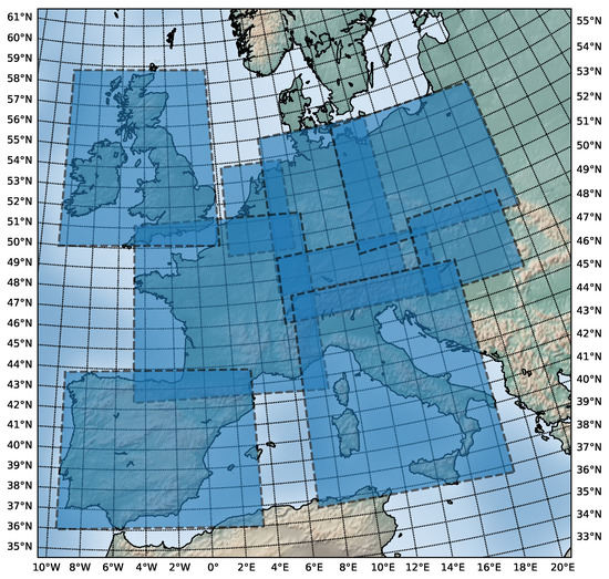
Figure 1.
Spatial extents used for nowcasting covering a total area of approximately 10.46 million km2, including the United Kingdom and Ireland (UK), Spain and Portugal (ES), France including Andorra and Monaco (FR), Switzerland and Austria (AT), Belgium, The Netherlands and Luxembourg (NL), Italy (IT), Germany (DE), Poland and the Czech Republic (PL), Hungary and Slovakia (HU).
This resulted in a total size of the processed dataset comprising 66 GB of sequence data. Furthermore, it is important to note that the MSG-CPP product relies on solar backscattered radiation, thus limiting observations to daytime (where the solar zenith angle is smaller than 78 degrees). Thus, an algorithm was developed, which, for each day, selected the optimal time range for a given spatial extent that satisfied the solar zenith constraint. All data preprocessing was carried out in parallel across 48 Intel Xeon Scalable processors (3.6 GHz) on the AWS cloud platform.
3. Methodology
3.1. Eulerian and Lagrangian Persistence
The baseline forecasting model consisted of assuming future cloud fields to be the same as the most recent observation, also called Eulerian persistence (Equation (1)), and representing the model expected to perform the worst [25].
Here, represents the observed cloud field, the start time of the forecast, with being the predicted field values at a given lead time and at a specific position x. Building on this notion, one can introduce Lagrangian persistence [25], which assumes that the state of each air parcel is constant, with all future change being due to parcels moving with the background flow (advection). Eulerian persistence can be extended to account for this by introducing an additional term that describes the displacement vector between consecutive fields as shown by Equation (2).
In this model, the predicted field at any given timestamp is equal to advecting by the semi-Lagrangian displacement vector , which can also include rotational motion [25].
3.2. Computing Displacement with Optical Flow
The displacement vectors u and v dictate the motion of a point in an image in the x and y directions, respectively, which can also be written as
with representing the pixel’s position, t being the time step and representing the change in a given variable. Optical flow thus is a technique used to compute motion vectors u and v from consecutive image frames, by calculating the distribution of apparent velocities of pixel intensities in an image. The first constraint of optical flow is that pixel intensities are constant between consecutive frames, with this assumption given by Equation (4).
Here, refers to the pixel intensity of a single point in the image at position at time t. As seen in this equation, pixel intensities for a tracked point are assumed to stay constant across consecutive frames. The next assumption of optical flow is that motion is small between consecutive frames so that the change in pixel intensities can be linearly approximated by taking the first-order derivatives of the pixel intensities and adding them to the initial pixel intensities as seen in Equation (5), which provides the small motion assumption.
We can then subtract Equation (4) from Equation (5), dividing this result by to yield the final optical flow Equation (6) with the two unknown displacement vector components u and v.
A common way to solve Equation (6) is through the Lucas–Kanade method, which uses least squares optimization to find the displacement vectors u and v [26]. This method is often used to track sparse features between images; however, due to the dynamic nature of clouds and the difficulty of identifying meaningful features to track across frames, dense optical flow algorithms were instead used according to Ayzel et al. [27], which compute the flow at all pixel locations in an image at each time step. Overall, three different optical flow algorithms were applied to the problem of nowcasting cloudiness.
3.2.1. Farneback
This method approximates the neighbourhood of frames using a polynomial expansion and estimates motion by computing orientation tensors by observing how polynomials transform under translation [28].
3.2.2. DeepFlow
DeepFlow blends a feature-matching algorithm with a variational optical flow approach. Features between frames are matched using a descriptor matching algorithm, which incorporates convolutions and max-pooling [29].
3.2.3. Dense Inverse Search (DIS)
This algorithm uses an inverse compositional image alignment (inverse Lucas–Kanade algorithm) to find patch correspondences and applies a densification step to compute a dense displacement field [30].
3.2.4. Ensemble Model
Finally, all three algorithms were merged into an ensemble model where at each time step of the nowcast, an average of all optical flow predictions was computed as defined in Equation (7).
Here, the ensemble prediction at a given lead time at position was computed as the average across all K optical flow algorithm predictions () for their respective lead time. Although these aforementioned optical flow methods are representative of the current state-of-the-art in non-deep-learning-based nowcasting models, they lack the ability to take into account advection patterns seen across multiple time steps and across multiple cloud evolution sequences. In order to better model such a variation, the use of a convolutional autoencoder network with gated recurrent units (ConvGRU) is proposed, which enables us to efficiently reconstruct the input sequences whilst also taking into account spatiotemporal dependencies.
3.3. Convolutional Gated Recurrent Unit Network
When using a deep neural network for nowcasting, the task of the network is to encode a sequence of past observations with input length t into a lower dimensional representation, followed by decoding these latent features to generate the most likely sequence of predictions with length , resulting in an input–output sequence akin to
The deep learning model architecture was based on an implementation of the ConvGRU model used for precipitation nowcasting by Shi et al. [31], which took a fixed length input sequence (4 frames in our case) and mapped it to an output sequence (12 frames in our case). The encoder processed a sequence of inputs (192 × 192) and downsampled it using various convolutional layers, creating a latent feature representation, which was upsampled in the decoder and mapped to the fixed output sequence using deconvolutions as depicted in Figure 2.
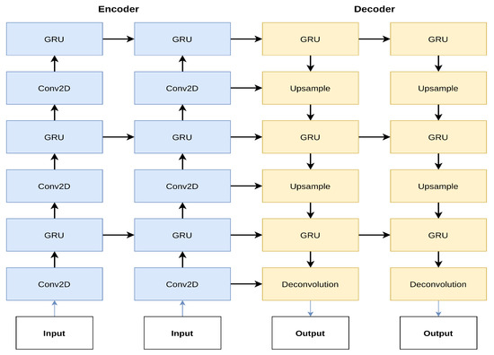
Figure 2.
Diagram of the convolutional gated recurrent unit model (ConvGRU) with three GRU units. Sequences are downsampled using convolutions (Conv2D), using a kernel size of 3 and a stride of 1, 2, 2 (bottom to top layer). Upsampling is done using transpose convolutions using a kernel size of 4 and a stride of 1, 2, 2, respectively, with all filter sizes being 64, 96, 96. This figure shows the model architecture when predicting a sequence of length 2. Figure was adapted from [31].
To retain spatiotemporal information and make predictions for each corresponding lead time, gated recurrent units (GRU) were used that are a gated version of recurrent units and modulate how information flows through the network through the implementation of sigmoid gates, allowing long-term temporal dependencies to be learned [32], with the main formulas for the GRU unit defined as follows:
Here, the inputs , where refers to the input channel and H and W to the respective height and width of the input image with t representing the time step. The update gate controls how much information from the previous time steps is carried forward, while the reset gate determines how much information to forget from previous time steps, which occurs by taking the Hadamard (elementwise) product between the reset gate and when calculating the candidate hidden state [32]. The candidate hidden state thus determines what elements of the previous hidden state to incorporate. Finally, is used to compute the final hidden state , which uses to control how much new information is written to the final state. As the activation function for the candidate hidden state, the Leaky rectified linear unit (ReLU) function with a negative slope of 0.2 denoted by f was used, while for the reset and update gates, the sigmoid activation function was applied, denoted by . Note that ⊙ refers to the Hadamard product and ∗ to the convolution operation.
3.4. Sequential Loss Functions
We introduce a novel sequential and locally oriented loss function to overcome the blurry image problem observed by previous work in the cloud nowcasting domain when using globally oriented loss functions such as MSE and MAE in convolutional autoencoders [20,21,22,23,33].
Central to our sequential loss function is the structural similarity index measure (SSIM). The SSIM measures nonstructural distortions (luminance and contrast changes) as well as structural changes, by computing similarity metrics between local image patches taken from the same location across three main image statistics, repeating this across the whole image using sliding windows, and finally averaging all local SSIM values yielding a global value for the image [34]. This metric was chosen as -based metrics such as the L1 or L2 norm, when used in the context of computing image fidelity, make the assumption that signal fidelity is independent of temporal or spatial relationships, thus failing to take into account image textures or patterns that occur between signal samples [34]. At a pixel level, SSIM can be defined as
where a and represent two non-negative image signals at identical locations between two images with a window size of 11 × 11 pixels. Furthermore, and correspond to the respective sample mean and standard deviation and represents the sample cross-correlation between a and . and are constants used to stabilise terms to prevent numerical instability [34,35]. Note that the SSIM metric was applied locally over the images using the aforementioned sliding window (11 × 11) with the mean value of all local computations over the two images being compared corresponding to their SSIM.
In our custom loss function, SSIM was calculated between each predicted image and the ground truth in each input sequence, whilst obtaining an average SSIM for the given sequence. This was repeated for all sequences in a batch, finally yielding a mean SSIM across all sequences in a batch giving an indication on how structurally similar sequences were to each other in a given batch. Note that as SSIM is usually a quantity to be maximised (between 0 and 1), we subtracted our loss from 1 as the gradient descent algorithm aimed to minimise our loss function given as:
where is our sequential SSIM loss function, B the number of batches with b referring to the batch index. T refers to the number of timestamps within a sequence with t representing the current timestamp and and being the predicted and actual cloud field.
3.5. Model Training and Evaluation
The optical flow nowcasts were carried out in parallel across 48 Intel Xeon Scalable processors (3.6 GHz) on the AWS cloud platform. Training of the deep learning models was done on an Nvidia V100 GPU with 16 GB memory. All models and logic were containerised using Docker allowing for multiple experiments to be run independently and in a reproducible way. The ConvGRU models were trained on 817 days of data across 9 different regions, which after optimising for optimum solar zenith angles yielded a total of 6694 three-hour sequences of length 16 (total of 107,104 observations). The models were all trained using a batch size of 6 over 3000 epochs with 5 different loss functions, effectively carrying out an ablation study of different loss functions. These included MAE, MSE, The Huber loss function (combination of L1 and L2 loss), our sequential SSIM loss and a combination of the sequential SSIM loss with MAE given as:
The length of the input sequences for both the optical flow and deep learning models were 4 frames (representing 1 h), with the nowcast lead time being 12 frames (3 h). The optimiser used for training was the AMSGrad variant of the Adam optimisation algorithm [36] with a constant learning rate of . Both the optical flow and deep learning approaches were evaluated by comparing nowcasts made for the same set of previously unseen test data spanning 205 days, which after solar zenith processing consisted of 1669 three-hour sequences across 9 different regions (total of 26,704 observations). Both the training and test datasets contained records sampled evenly across all meteorological seasons as can be seen in Figure 3. Evaluation metrics were computed by comparing actual versus predicted cloud fields using the coefficient of determination (), mean absolute error and finally also by calculating the structural similarity index.
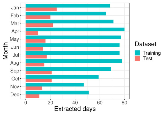
Figure 3.
Distribution of the training and test sets which was selected to contain an equal distribution across meteorological seasons to account for seasonal variation in cloud dynamics within the dataset.
4. Results and Discussion
4.1. Optical Flow vs. ConvGRU Nowcasts
Optical flow provided a viable way to nowcast clouds with a lead time of 3 h. The three different optical flow algorithms (DeepFlow, Dense Inverse Search and Farneback) all showed significantly better performance than the persistence baseline model, with an on average increase in , and across all three models of 10.75%, −10.41% and 3.09, respectively, for all time steps. However, as can be seen in Table 1, there were differences in the predictive power between the three individual optical flow models (DeepFlow, DIS, Farneback). The DIS model yielded the smallest improvements across all metrics compared to the persistence model and was the worst-performing optical flow model overall. In addition, as can be seen in Figure 4, the SSIM of predictions made with the DIS model degraded the fastest out of all models and in fact became worse than the persistence model after a lead time of 75 min. DeepFlow and Farneback both outperformed DIS; however, they showed consistently different results across metrics. Farneback yielded predictions with a better SSIM, whilst DeepFlow based predictions showed a better and MAE throughout all time steps, however, with a SSIM worse than the persistence model after 120 min.

Table 1.
Average percentage differences in accuracy metrics of optical flow predictions against the persistence baseline, grouped by lead time ().
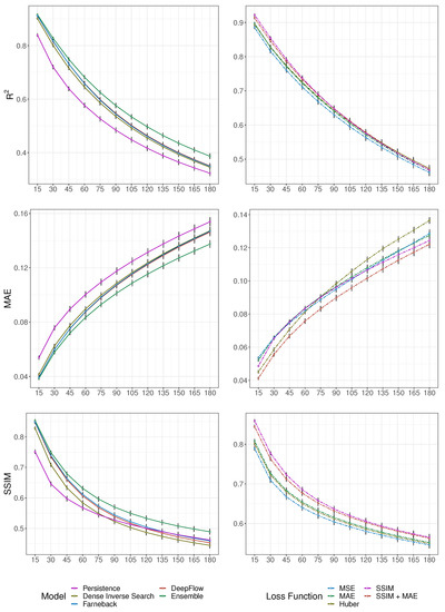
Figure 4.
A comparison of average model performance across all lead times in the test set, for all optical flow models and the persistence baseline (left) and the ConvGRU based models with varying loss functions (right). Results show cumulative mean accuracy metrics per lead time in minutes.
Importantly, however, the ensemble of optical flow algorithms yielded an on average increase in , and of 17.82%, −15.61% and 9.14%, respectively across all time steps, representing the best-performing optical flow model. As can be seen in Table 1 and Figure 4, the ensemble model consistently outperformed all other optical flow models for all metrics at all time steps with an average change over the persistence model at a lead time of three hours of 19.73%, −10.67% and 5.89% for , and , respectively. A multiple comparison of accuracy metrics between optical flow methods using the pairwise Wilcoxon rank sum test with a Benjamin and Hochberg adjustment confirmed that the ensemble model displayed significantly higher scores for , when compared to all other optical flow models. This difference though was not statistically significant for and .
In comparison, we found that the ConvGRU models showed a consistently better performance than the ensemble optical flow model. The average improvement in the best performing ConvGRU model (trained with both the SSIM and MAE loss functions) yielded an on average improvement in , and over the ensemble optical flow model of 12.43%, −8.75% and 9.68% across all time steps, respectively. Furthermore, as can be seen in Table 2 there were large differences in predictive performance between the ConvGRU models trained with locally oriented loss functions such as our SSIM loss function, versus models trained with global loss functions such as MSE. The models trained with the and loss showed a significantly higher improvement in performance over the ensemble optical flow model in terms of MAE and SSIM. However, in terms of alone, the ConvGRU model trained solely with the SSIM loss function yielded the highest SSIM scores out of all models for all time steps, and consequently also produced the most blur-free predictions as can be seen in an example prediction in Figure 5.
Table 2.
Average percentage differences in accuracy metrics of ConvGRU predictions against the optical flow ensemble baseline, grouped by lead time ().
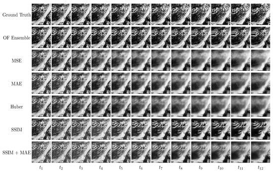
Figure 5.
An example 3 h nowcast (12 frames) over France on 17 March 2019, contrasting the ensemble optical flow model and ConvGRU-based nowcasting models trained with different loss functions against the ground truth sequence, with representing each 15 min time step. Here, the OF ensemble is the worst performing model, with the best performing model being the SSIM model.
4.2. Regional Effects on ConvGRU Performance
In addition to a variation in predictive performance across time, a significant geographical variation in performance was observed across different ConvGRU models as can be seen in Figure 6. We computed the standard deviation of the mean percentage change with respect to the ensemble optical flow model and observed various levels of variance between different regions. In particular, the highest variances were observed in the MAE metric (where ), indicating that this metric was sensitive to the geographical location and chosen loss function. In particular, the highest spread in MAE was observed in Spain, Italy and France with equal to 0.17, 0.14 and 0.12, respectively, which can be observed by the large spread in across ConvGRU models for those countries in Figure 6. Here, it can also be seen that for forecasts with a lead time under 1 h in terms of MAE, the models trained using globally oriented loss functions such as MSE and Huber were outperformed by the optical flow ensemble model for that lead time, except for the model, which outperformed all others after the first 15 min.
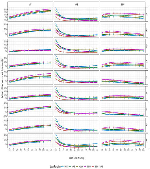
Figure 6.
Regional differences in cumulative mean accuracy metrics for all lead times across all ConvGRU based models. Results show the mean percentage change with respect to the optical flow ensemble model for each time step.
With regards to the SSIM metric, we found that it was less sensitive to geographical variation, with ranging between 0.04 and 0.07 across all evaluated geographical regions. As seen in Figure 6, the highest spread in ConvGRU model performance was observed in Switzerland and Austria, the United Kingdom and France, indicating that here, the use of locally oriented loss functions was particularly useful to enhancing predictive performance for that specific metric. For this metric, the ConvGRU model trained using SSIM showed the consistently highest improvement over the ensemble optical flow model for all time steps across all tested regions.
was not as affected by regional changes; however, it had the highest differences within model performance found across the Netherlands, Switzerland and Austria with variances of 0.1 each. For this metric the ConvGRU model trained with SSIM loss again showed the highest performance across all time steps for all regions, except for Spain. In the case of Spain, the SSIM model performed the best for the first 30 min, followed by the SSIM + MAE model from 30 to 105, with the MSE model finally performing the best by a small margin between a lead time of 105 and 180 min.
Key Findings
This study showed that optical flow and deep learning algorithms provided accurate ways of nowcasting cloud motion for the next three hours. In particular, it was shown that dense optical flow algorithms that track global pixel displacement could be used for nowcasting of said properties with good near-term forecasting accuracy (1 h) as can be seen in Table 1 and Figure 4. These findings were in accordance with results from Ayzel et al. [27], who showed that dense optical flow algorithms could be successfully applied to nowcasting precipitation fields, whereas in our case we showed that an ensemble of optical flow models performed better than any individual model. This may have been the case as each individual model contained built-in assumptions whose errors could be modelled as additive independent and identically distributed noise, where a noisy image consisted of the real image and the added noise with corresponding to the spatial image coordinates [37] as shown by:
It then followed that conventional image merging methods could be applied to effectively denoise the different optical flow nowcasts to obtain more accurate predictions by averaging out the additive noise which can be written as:
When following the additive noise model, the underlying image stayed constant whilst averaging over multiple images reduced the noise term , as it tends to a mean of zero if assumed to follow a standard normal distribution [37]. However, one of the main drawbacks we observed from using optical flow, was that it could result in image-warping artefacts along the displacement vectors that distorted the image and reduced forecast quality as can be observed in Figure A2, Figure A6 and Figure A7.
Furthermore, our results also confirmed that ConvGRUs trained with a combination of local and global loss () outperformed optical flow at time scales larger than 15 min in terms of MAE and for all time scales for and . The improvements were particularly pronounced when using a combination of locally and globally oriented loss functions (), as well as only , overall yielding the greatest performance improvements, and effectively yielding a solution to the blurry image problem reported previously when only using global loss functions as the optimisation criterion of the nowcasting model [20,21,22,23,33]. These results were in line with similar findings in the precipitation nowcasting domain [38], with our custom sequential loss function, which combined a sequential structural similarity measure and mean absolute error, striking the balance between preserving global and local loss. This resulted in the best overall performance across our evaluation metrics with average increases over the ensemble optical flow model at a lead time of 3 h of 22.21%, −11.18% and 15.07% for , and , respectively, for the model, and 21.10%, −9.48% and 15.53% for the model (see Table 2). Finally, we showed that with the addition of locally oriented loss functions our predictions produced nowcasts with significantly higher SSIM scores compared to cloud nowcasts by Knol et al., who used MSE as the main optimisation criterion [21].
We also confirmed that models trained using our custom loss functions (, ) consistently performed the best across all geographical regions in our dataset (see Figure 6). Interestingly, we also observed a variation across geographical regions which may be linked to varying land-surface characteristics and local weather variability, which may contribute to the difficulty of the overall nowcasting task. Our custom loss functions were deemed especially performant in mountainous areas, which display a number of complex cloud formation processes such as orographic lifting and others, therefore making the resulting cloud fields more heterogeneous, and therefore making a more important metric to optimise for. Conversely, in high-pressure and less climatologically variable regions such as Spain, the observed effect of switching between models optimised for structural similarity yielded smaller gains. In the context of other research using deep-learning-based models such as ConvLSTMs and U-Net-based architectures for precipitation nowcasting [16,18,39], we also showed that deep learning could be applied for nowcasting cloud fields, with significantly improved forecasts made possible by introducing an optimisation criterion which also took into account the preservation of image structure, which thus far has not been accounted for in the cloud nowcasting literature. Structural improvements in the forecasts were also visible in generated sequences themselves. Examples of this can be seen in Figure 7 below, as well as in Figure A2–Figure A6. In particular, in Figure 8, it can be clearly seen that the MSE-trained model blurred the forecast to reduce the mean forecast error, whereas the SSIM-trained model better maintained the structure of the last observed cloud field. However, although our models learned to advect cloud fields over time other cloud formation processes were not captured. In Figure 9, convective initiation over the European Alps is observed, with none of the models able to also grow clouds accordingly.
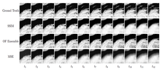
Figure 7.
Example 3 h nowcasts over Poland on 29 September 2020.
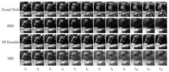
Figure 8.
Example 3 h nowcasts over the Netherlands on 9 June 2018.
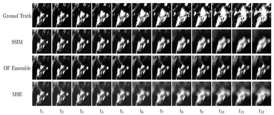
Figure 9.
Example 3 h nowcasts over Austria and Switzerland on 1 July 2019.
In summary, although we provided a solution to the blurry image problem, we still observed limitations in our model’s generalisation ability across different regions due to their different climatic characteristics, meaning that the inclusion of additional data sources may further improve forecasts, and potentially also across different cloud types which are the result of cloud formation processes other than advection. In the future, we envision the extension of our model using a multimodal training framework, incorporating a variety of different data sources which may help the model better capture cloud microphysics and cloud formation processes which vary by geographical region due to different local land surface characteristics. For this, we foresee the incorporation of detailed topographical elevation data, land surface cover, and other climate characteristics such as temperature and wind direction. Additionally, given that our dataset currently generalises the presence of clouds as a function of available solar radiation, we also cannot currently determine the performance of our model across different cloud types (e.g., cirrus, cumulus, stratus), as well as its performance on clouds at different heights in the atmosphere. Therefore, we also foresee that our future training dataset should incorporate such discriminating features so that the model will be able to also be evaluated on those. Furthermore, even though we conducted an ablation study of loss functions, and thereby determined the usefulness of locally oriented loss functions, we aim to extend this in future research. In particular, it would be useful to vary the number of GRU units in the network, as well as the kernel size, stride and filter sizes using hyperparameter optimisation. In addition, we also foresee the usage of a larger spatial input data context to be useful when making longer predictions into the future. Furthermore, it would also be beneficial to study the effect of using attention mechanisms as this approach has shown to yield very good results for extended forecast horizons of up to 12 h in the context of precipitation nowcasting [18,19].
5. Conclusions
In this study, the use of multiple optical flow algorithms and ConvGRUs to nowcast clouds for the next 3 h using MSG-CPP satellite data was investigated. One of the main contributions was to show that the introduction of a sequential loss function which took into account both image structure and global loss significantly increased the predictive performance of ConvGRUs when nowcasting clouds. Furthermore, it was observed that through this approach the blurry image problem highlighted by previous research could be overcome and as a result more structurally accurate nowcasts could be generated. With regards to optical-flow-based approaches, we also showed that these could be enhanced through the use of image-merging techniques, yielding a good nowcasting accuracy for short timescales of up to 1 h.
Nonetheless, our study also highlighted some limitations in the application of deep learning to cloud nowcasting. Although our ConvGRU models learned to advect cloud fields, they were not able to thoroughly model other cloud formation processes such as convection and orographic lifting. Furthermore, results on our training dataset cannot be directly extrapolated to expected cloud nowcasting performance for different cloud types at different heights in the atmosphere, as our dataset provided a general proxy for cloudiness by means of solar radiation. As such, in future studies, an emphasis should not only be placed on improvements in the model architecture, but also on the curation of training data enabling cloud nowcasting at a more granular level.
Overall, our findings pave the way to use deep learning to generate longer and more accurate nowcasts and help operationalise deep learning based nowcasting approaches for a variety of use cases such as for solar-power forecasting. Our deep learning model learned to represent advection of clouds over time and was able to represent their structure. Overall, this study shows that deep-learning-based models will be able to greatly enhance future operational nowcasting systems, and that it is possible to apply them to a wide range of different nowcasting problems. It is envisioned that future renewable energy generation forecasting systems will be able to greatly benefit from the integration of deep-learning-based nowcasting models such as the one presented here.
Author Contributions
Conceptualization, S.A.K., F.D.L. and C.R.R.; methodology, S.A.K. and F.D.L.; software, S.A.K. and F.D.L.; validation, S.A.K.; formal analysis, S.A.K.; investigation, S.A.K.; resources, S.A.K. and F.D.L.; data curation, S.A.K. and F.D.L.; writing—original draft preparation, S.A.K.; writing—review and editing, S.A.K.; visualization, S.A.K.; supervision, F.D.L. and C.R.R.; project administration, S.A.K., F.D.L. and C.R.R.; funding acquisition, F.D.L. and C.R.R. All authors have read and agreed to the published version of the manuscript.
Funding
The APC was funded by the University of Amsterdam and Dexter Energy Services B.V.
Institutional Review Board Statement
Not applicable.
Informed Consent Statement
Not applicable.
Data Availability Statement
Not applicable.
Conflicts of Interest
The authors declare no conflict of interest.
Appendix A. Example Training Data

Figure A1.
Example 4 h sequence from the training dataset showing direct surface solar irradiance extracted from the MSG-CPP dataset assuming clear sky (a), and without assuming clear sky (b), with (c) showing the normalised solar radiation used as a proxy for cloudiness (with values between 0 and 1). Darker regions show higher solar radiation while lighter regions represent lower solar radiation. represent the input frames used to train the models, while represent the target frames.
Appendix B. Example Nowcasts
Herein are presented example 3 h nowcasts (includes twelve frames with each frame corresponding to a 15 min time step) made on the unseen test dataset covering all extracted geographical regions in this study. The ground truth is shown along with the ConvGRU model trained with the SSIM and MSE loss as well as the ensemble optical flow model (OF ensemble).

Figure A2.
Example 3 h nowcasts over France on 2 May 2020.

Figure A3.
Example 3 h nowcasts over Spain on 5 September 2019.

Figure A4.
Example 3 h nowcasts over Germany on 6 January 2020.

Figure A5.
Example 3 h nowcasts over Italy on 31 March 2018.

Figure A6.
Example 3 h nowcasts over Hungary on 28 September 2019.

Figure A7.
Example 3 h nowcasts over the United Kingdom and Ireland on 20 July 2019.
References
- Schneider, T.; Teixeira, J.; Bretherton, C.S.; Brient, F.; Pressel, K.G.; Schär, C.; Siebesma, A.P. Climate goals and computing the future of clouds. Nat. Clim. Chang. 2017, 7, 3–5. [Google Scholar] [CrossRef]
- Quante, M. The role of clouds in the climate system. EDP Sci. 2004, 121, 61–86. [Google Scholar] [CrossRef]
- Wang, D.C.; Jacobs, J.; Nikitina, R.; Wang, W. Guidelines for Nowcasting Techniques; World Meteorological Organization: Geneva, Switzerland, 2017. [Google Scholar]
- Purdom, J.F.W. Some Uses of High-Resolution GOES Imagery in the Mesoscale Forecasting of Convection and Its Behavior. Mon. Weather Rev. 1976, 104, 1474–1483. [Google Scholar] [CrossRef]
- Siewert, C.W.; Koenig, M.; Mecikalski, J.R. Application of Meteosat second generation data towards improving the nowcasting of convective initiation. Meteorol. Appl. 2010, 17, 442–451. [Google Scholar] [CrossRef]
- Benas, N.; Finkensieper, S.; Stengel, M.; van Zadelhoff, G.J.; Hanschmann, T.; Hollmann, R.; Meirink, J.F. The MSG-SEVIRI-based cloud property data record CLAAS-2. Earth Syst. Sci. Data 2017, 9, 415–434. [Google Scholar] [CrossRef]
- Liu, Y.; Xi, D.G.; Li, Z.L.; Hong, Y. A new methodology for pixel-quantitative precipitation nowcasting using a pyramid Lucas Kanade optical flow approach. J. Hydrol. 2015, 529, 354–364. [Google Scholar] [CrossRef]
- Gallucci, D.; Romano, F.; Cersosimo, A.; Cimini, D.; Di Paola, F.; Gentile, S.; Geraldi, E.; Larosa, S.; Nilo, S.T.; Ricciardelli, E.; et al. Nowcasting Surface Solar Irradiance with AMESIS via Motion Vector Fields of MSG-SEVIRI Data. Remote Sens. 2018, 10, 845. [Google Scholar] [CrossRef]
- Woo, W.c.; Wong, W.k. Operational Application of Optical Flow Techniques to Radar-Based Rainfall Nowcasting. Atmosphere 2017, 8, 48. [Google Scholar] [CrossRef]
- Bowler, N.E.; Pierce, C.E.; Seed, A.W. STEPS: A probabilistic precipitation forecasting scheme which merges an extrapolation nowcast with downscaled NWP. Q. J. R. Meteorol. Soc. 2006, 132, 2127–2155. [Google Scholar] [CrossRef]
- Sirch, T.; Bugliaro Goggia, L.; Zinner, T.; Möhrlein, M.; Vazquez-Navarro, M. Cloud and DNI nowcasting with MSG/SEVIRI for the optimized operation of concentrating solar power plants. Atmos. Meas. Tech. (AMT) 2017, 10, 409–429. [Google Scholar] [CrossRef]
- Nouri, B.; Kuhn, P.; Wilbert, S.; Prahl, C.; Pitz-Paal, R.; Blanc, P.; Schmidt, T.; Yasser, Z.; Santigosa, L.R.; Heineman, D. Nowcasting of DNI maps for the solar field based on voxel carving and individual 3D cloud objects from all sky images. AIP Conf. Proc. 2018, 2033, 190011. [Google Scholar] [CrossRef]
- Paulescu, M.; Paulescu, E.; Badescu, V. Chapter 9—Nowcasting solar irradiance for effective solar power plants operation and smart grid management. In Predictive Modelling for Energy Management and Power Systems Engineering; Elsevier: Amsterdam, The Netherlands, 2021; pp. 249–270. [Google Scholar] [CrossRef]
- Song, S.; Yang, Z.; Goh, H.; Huang, Q.; Li, G. A novel sky image-based solar irradiance nowcasting model with convolutional block attention mechanism. Energy Rep. 2022, 8, 125–132. [Google Scholar] [CrossRef]
- Shi, X.; Chen, Z.; Wang, H.; Yeung, D.Y.; Wong, W.k.; Woo, W.c. Convolutional LSTM Network: A Machine Learning Approach for Precipitation Nowcasting. arXiv 2015, arXiv:1506.04214. [Google Scholar]
- Ayzel, G.; Scheffer, T.; Heistermann, M. RainNet v1.0: A convolutional neural network for radar-based precipitation nowcasting. In Geoscientific Model Development Discussions; 2020; pp. 1–20. [Google Scholar] [CrossRef]
- Su, A.; Li, H.; Cui, L.; Chen, Y. A Convection Nowcasting Method Based on Machine Learning. Advances in Meteorology 2020, 2020, 13. [Google Scholar] [CrossRef]
- Sønderby, C.K.; Espeholt, L.; Heek, J.; Dehghani, M.; Oliver, A.; Salimans, T.; Agrawal, S.; Hickey, J.; Kalchbrenner, N. MetNet: A Neural Weather Model for Precipitation Forecasting. arXiv 2020, arXiv:2003.12140. [Google Scholar]
- Espeholt, L.; Agrawal, S.; Sønderby, C.; Kumar, M.; Heek, J.; Bromberg, C.; Gazen, C.; Hickey, J.; Bell, A.; Kalchbrenner, N. Skillful Twelve Hour Precipitation Forecasts using Large Context Neural Networks. arXiv 2021, arXiv:2111.07470. [Google Scholar]
- Berthomier, L.; Pradel, B.; Perez, L. Cloud Cover Nowcasting with Deep Learning. In Proceedings of the 2020 Tenth International Conference on Image Processing Theory, Tools and Applications (IPTA), Paris, France, 9–12 November 2020; pp. 1–6. [Google Scholar] [CrossRef]
- Knol, D.; de Leeuw, F.; Meirink, J.F.; Krzhizhanovskaya, V.V. Deep Learning for Solar Irradiance Nowcasting: A Comparison of a Recurrent Neural Network and Two Traditional Methods. In Proceedings of the Computational Science—ICCS 2021, Krakow, Poland, 16–18 June 2021; Paszynski, M., Kranzlmüller, D., Krzhizhanovskaya, V.V., Dongarra, J.J., Sloot, P.M., Eds.; Springer International Publishing: Cham, Switzerland, 2021; pp. 309–322. [Google Scholar]
- Ionescu, V.S.; Czibula, G.; Mihuleţ, E. DeePS at: A deep learning model for prediction of satellite images for nowcasting purposes. In Knowledge-Based and Intelligent Information & Engineering Systems: Proceedings of the 25th International Conference KES2021, Szczecin, Poland, 8–10 September 2021; Volume 192, pp. 622–631. [CrossRef]
- Yang, Y.; Mehrkanoon, S. AA-TransUNet: Attention Augmented TransUNet For Nowcasting Tasks. arXiv 2022, arXiv:2202.04996. [Google Scholar]
- Greuell, W.; Meirink, J.F.; Wang, P. Retrieval and validation of global, direct, and diffuse irradiance derived from SEVIRI satellite observations. J. Geophys. Res. Atmos. 2013, 118, 2340–2361. [Google Scholar] [CrossRef]
- Germann, U.; Zawadzki, I. Scale-Dependence of the Predictability of Precipitation from Continental Radar Images. Part I: Description of the Methodology. Mon. Weather Rev. 2002, 130, 2859–2873. [Google Scholar] [CrossRef]
- Lucas, B.D.; Kanade, T. An iterative image registration technique with an application to stereo vision. In Proceedings of the 7th International Joint Conference on Artificial Intelligence, Vancouver, BC, Canada, 24–28 August 1981; Morgan Kaufmann Publishers Inc.: Burlington, MA, USA, 1981; Volume 2, pp. 674–679. [Google Scholar]
- Ayzel, G.; Heistermann, M.; Winterrath, T. Optical flow models as an open benchmark for radar-based precipitation nowcasting (rainymotion v0.1). Geosci. Model Dev. 2019, 12, 1387–1402. [Google Scholar] [CrossRef]
- Farnebäck, G. Two-Frame Motion Estimation Based on Polynomial Expansion. In Image Analysis. SCIA 2003. Lecture Notes in Computer Science; Bigun, J., Gustavsson, T., Eds.; Springer: Berlin/Heidelberg, Germany, 2003; Volume 2749, pp. 363–370. [Google Scholar] [CrossRef]
- Weinzaepfel, P.; Revaud, J.; Harchaoui, Z.; Schmid, C. DeepFlow: Large Displacement Optical Flow with Deep Matching. In Proceedings of the ICCV—IEEE International Conference on Computer Vision, 1–8 December 2013; pp. 1385–1392. [Google Scholar] [CrossRef]
- Kroeger, T.; Timofte, R.; Dai, D.; Van Gool, L. Fast Optical Flow using Dense Inverse Search. arXiv 2016, arXiv:1603.03590 [cs]. [Google Scholar]
- Shi, X.; Gao, Z.; Lausen, L.; Wang, H.; Yeung, D.Y.; Wong, W.k.; Woo, W.c. Deep Learning for Precipitation Nowcasting: A Benchmark and A New Model. arXiv 2017, arXiv:1706.03458 [cs]. [Google Scholar]
- Chung, J.; Gulcehre, C.; Cho, K.; Bengio, Y. Empirical Evaluation of Gated Recurrent Neural Networks on Sequence Modeling. arXiv 2014, arXiv:1412.3555 [cs]. [Google Scholar]
- Fernández, J.G.; Mehrkanoon, S. Broad-UNet: Multi-scale feature learning for nowcasting tasks. Neural Netw. 2021, 144, 419–427. [Google Scholar] [CrossRef]
- Wang, Z.; Bovik, A.C. Mean squared error: Love it or leave it? A new look at Signal Fidelity Measures. IEEE Signal Process. Mag. 2009, 26, 98–117. [Google Scholar] [CrossRef]
- Wang, Z.; Bovik, A.; Sheikh, H.; Simoncelli, E. Image Quality Assessment: From Error Visibility to Structural Similarity. IEEE Trans. Image Process. 2004, 13, 600–612. [Google Scholar] [CrossRef]
- Phuong, T.T.; Phong, L.T. On the Convergence Proof of AMSGrad and a New Version. IEEE Access 2019, 7, 61706–61716. [Google Scholar] [CrossRef]
- Bovik, A. Handbook of Image and Video Processing, 2nd ed.; Elsevier: Amsterdam, The Netherlands, 2005. [Google Scholar]
- Tran, Q.K.; Song, S.K. Computer Vision in Precipitation Nowcasting: Applying Image Quality Assessment Metrics for Training Deep Neural Networks. Atmosphere 2019, 10, 244. [Google Scholar] [CrossRef]
- Kumar, A.; Islam, T.; Sekimoto, Y.; Mattmann, C.; Wilson, B. Convcast: An embedded convolutional LSTM based architecture for precipitation nowcasting using satellite data. PLoS ONE 2020, 15, e0230114. [Google Scholar] [CrossRef]
Publisher’s Note: MDPI stays neutral with regard to jurisdictional claims in published maps and institutional affiliations. |
© 2022 by the authors. Licensee MDPI, Basel, Switzerland. This article is an open access article distributed under the terms and conditions of the Creative Commons Attribution (CC BY) license (https://creativecommons.org/licenses/by/4.0/).