Abstract
This paper provides an Extreme Value Analysis (EVA) of the hourly water level record at Fort Denison dating back to 1915 to understand the statistical likelihood of the combination of high predicted tides and the more dynamic influences that can drive ocean water levels higher at the coast. The analysis is based on the Peaks-Over-Threshold (POT) method using a fitted Generalised Pareto Distribution (GPD) function to estimate extreme hourly heights above mean sea level. The analysis highlights the impact of the 1974 East Coast Low event and rarity of the associated measured water level above mean sea level at Sydney, with an estimated return period exceeding 1000 years. Extreme hourly predictions are integrated with future projections of sea level rise to provide estimates of relevant still water levels at 2050, 2070 and 2100 for a range of return periods (1 to 1000 years) for use in coastal zone management, design, and sea level rise adaptation planning along the NSW coastline. The analytical procedures described provide a step-by-step guide for practitioners on how to develop similar baseline information from any long tide gauge record and the associated limitations and key sensitivities that must be understood and appreciated in applying EVA.
1. Introduction
The threat of rising mean sea-level (MSL) associated with climate change will be profound, with extensive biophysical, ecological, social, and economic impacts forecast. From a purely asset and infrastructure-based perspective, it has been estimated that some $226 billion in commercial, industrial, road, rail, and residential assets are likely at risk around Australia from sea level rise alone by 2100, if greenhouse gas emissions continue at high levels [1].
It has been estimated that historical greenhouse gas emissions between 1750 and 2016 will result in a committed global mean sea-level (GMSL) rise of around 1 m between the present and 2300 [2]. The recently released forecasts from modelling provided by the Intergovernmental Panel on Climate Change (IPCC), suggest that under a high emission scenario (e.g., SSP5-8.5), GMSL rise could be of the order of a metre this century alone [3].
Over the past decade, planning and adaptation to respond to current and projected climate change induced rises in GMSL have taken on greater prominence and sophistication at increasingly localised scales. Not only have techniques advanced to isolate the low-frequency MSL signal with improved temporal resolution from tide gauge records (e.g., [4]), but considerable research effort has improved understanding of the associated impacts of higher frequency, dynamic sea level extremes [5]. Extremes can be considered as a combination of a wide variety of largely unrelated dynamic oceanographic effects over differing timescales, from shorter duration storm surges, shelf waves, inverse barometer effect, etc., through to longer timescale influences including fluctuations in ocean currents, density, salinity and temperature changes in sea water, through to even longer timescale influences including climate modes (such as ENSO, PDO, IOD, etc.) superimposed on predicable tidal responses.
Understanding the statistical likelihood of extreme water levels driven by high predicted tides coinciding with these more dynamic influences that can drive ocean water levels higher at the coast, is of primary interest for coastal design, planning and engineering purposes. Integrating this information with future projections of sea level rise provides some assurance that adequate design parameters can be applied to the proposed lifecycle of the task at hand.
The scale of these high frequency dynamic influences can vary considerably from location to location, dependent primarily on relevant regional scale oceanographic and storm system drivers. For example, along the NSW coastline, the principal influences elevating ocean waters above the predicted tide include barometric and wind setup as well as coastally trapped waves which migrate south to north along the coast over generally 2–3 days. These combined influences have been measured in the order of up to 0.8 m [6]. Further north in the state of Queensland, high frequency influences associated with tropical cyclone activity can elevate the ocean water levels several metres above the predicted tide due to storm surge driven by extreme winds and low central pressures. In 2011, Tropical Cyclone “Yasi” devastated large stretches of the Queensland coast where the maximum recorded storm surge exceeded 5 m [7].
Studies over more recent years have become more nuanced around integrating projected sea level rise with these more dynamic influences to highlight the increasing risks associated with tidal flooding phenomena. Various studies highlight the influence of longer period tidal variations for localised flooding around the USA (e.g., [8,9]), whilst other studies note the more regionally specific dynamic influences affecting extreme sea levels in various locations [10,11,12]. Numerous studies advise the intensification in the frequency of oceanic inundation events anticipated by sea level rise projections over various time horizons (e.g., [13,14]).
This study looks specifically at the long Fort Denison tide gauge record at Sydney, Australia (refer Figure 1) with high frequency (hourly) data available from 10 June 1914 (0400 h) for analysis. This paper is focused on understanding the peak heights (or extremes) measured above MSL resulting from the coincidence of predictable tides and high frequency dynamic influences.
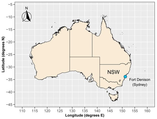
Figure 1.
Locality Plan (Fort Denison, Sydney).
Statistical techniques associated with Extreme Value Analyses (EVA) have been well developed in the literature (e.g., [15,16,17,18,19,20,21,22,23]) with the ‘Block Maxima’ (BM) and ‘Peaks-Over-Threshold’ (POT) approaches being the most popular. Both parametric modelling approaches involve the fitting of continuous probability distribution functions based on variations of asymptotic tails which are used to predict rare (or extreme) phenomenon often well beyond the boundary of the measured data. The earliest application of the POT approach can be traced to work in the hydrology sector [24]. The POT approach is considered more advantageous in fitting natural phenomena as it includes all independent events above a prescribed threshold, whereas the alternative BM approach is based on selection of a single maxima per equidistant time segments, ignoring other key rare events occurring within the same time segment [20]. By virtue, The BM method has often been considered a wasteful approach to EVA if other data on extremes are available [25]. Hence this study uses the POT approach.
The POT method consists of fitting the Generalised Pareto Distribution (GPD) to the peaks of declustered excesses over a defined threshold [26]. The GPD contains a family of probability distribution functions which converge to one of three separate asymptotic tailed solutions, namely: a heavy tail; light tail; or bounded tail approximation. The optimum distribution is selected by means of fitting the empirical data with the use of shape and scale parameters. Whilst the POT offers advantages over the BM approach, the reliance of the technique on selection of an appropriate threshold above which to analyze extreme measured data has been considered a limitation. However, several works in the literature provide outstanding guidance on best practice applications for the POT technique (e.g., [26,27,28]) for natural phenomena.
Whilst this guidance has been observed, this paper offers two important improvements. Firstly, the necessary detrending of the source data takes advantage of recent advancements in estimating and removing the MSL trend from long tide gauge records (e.g., [4,29]). Secondly, this study proposes the application of an improved diagnostic approach to selection of an optimised threshold level for POT based on the consideration of several independent tests and analytical outcomes. These approaches have been largely automated using the ‘extRemes’ extension package in R [30,31,32].
The optimal fitted GPD function has been used to estimate design peak water level heights above MSL, for return periods ranging from 1 to 1000 years. These estimates have been integrated with the most up to date sea level projections from the IPCC (AR6), to provide improved design still water levels (SWLs) for planning, design, and climate adaptation purposes for Sydney to 2100. The underpinning methodology has useful application for practitioners at any coastal location where lengthy high frequency (hourly) data is available.
The paper is structured with a detailed explanation of the analytical methodologies applied and the data used (Section 2), leading into a presentation of the results of the updated analysis (Section 3), a discussion section including key thoughts regarding sensitivity analyses (Section 4), and finally, conclusions are provided (Section 5).
2. Materials and Methods
Various data sources and methodologies have been applied in the study and are described in detail in the following sections.
2.1. Data Sources Used in the Study
A range of data sources have been used to facilitate different parts of the analysis. Annual average time series data for Fort Denison from the public archives of the Permanent Service for Mean Sea Level (PSMSL) [33,34] (Station ID = 196) have been used in the MSL analysis spanning the period from 1915 to 2020 (inclusive).
Hourly tide gauge observations for Fort Denison spanning the period from 10 June 1914 (0400 h) to 31 December 1994 (2300 h) have been made available by the National Operations Centre (NOC) Tidal Unit, Australian Bureau of Meteorology. Hourly observations spanning the timeframe from 1 January 1965 (0100 h) to 30 June 2021 (2300 h) have been sourced from the University of Hawaii, Sea Level Centre (UHSLC) [35,36] (Station ID = 333).
Sea level projections for a range of Shared Socioeconomic Pathway (SSP) scenarios have been sourced directly from the IPCC [3]. Specifically, data for Figure SPM8 (Panel d: Global mean sea level change relative to 1900) provide global averaged sea level projections at decadal intervals between 2020 and 2100 for the five modelled SSPs (SSP1-1.9, SSP1-2.6, SSP2-4.5, SSP3-7.0 and SSP5-8.5) as summarised in Table 1.

Table 1.
Summary of Projected Sea Level Rise under Different SSP Scenarios (mm).
2.2. Step by Step Methodology
The analytical steps involved in estimating extreme sea levels at Sydney for design and planning purposes over differing planning horizons are detailed in the following sections. All analysis and graphical outputs have been developed by the author from customised scripting code within the framework of the R Project for Statistical Computing [30].
Step 1: Determination of MSL trend. This is a critical initial step as the fitting of a GPD function to estimate extreme values is based on the statistical principles of stationarity. The key task with this step is to isolate the comparatively small, non-stationary, non-linear MSL signal from the significant and substantial dynamic inter-decadal (and other) influences and noise. This is achieved through the application of Singular Spectrum Analysis (SSA) techniques adapted specifically for MSL research [29,37] which have been further refined and applied to large regional studies of long tide gauge records [4,38]. The process uses annual average MSL time series data from the PSMSL, where the data time series has been adjusted to reflect the midpoint of each year.
The SSA procedure requires a complete time series, therefore the three missing annual average values at Fort Denison (1930, 1941 and 2000) have been filled using an iterative SSA procedure [39] which has an (assumed) advantage in preserving the principal spectral structures of the complete portions of the original data set in filling the gaps.
The complete time series is then decomposed using one-dimensional SSA to isolate components of slowly varying trend (i.e., MSL) from oscillatory components with variable amplitude, and noise. A technique known as frequency thresholding [40] is then used to aggregate components from the SSA decomposition that have “trend-like” characteristics. In general, the trend of MSL associated with external climate forcing can be considered to comprise components in which more than 50% of the relative spectral energy resides in the low-frequency band between 0 and 0.02 cycles per year, which accord with the findings of Mann et al. [41].
The isolated MSL signal is then fitted with a cubic smoothing spline model to permit prediction of MSL at each hourly time step over the time span of the data (1915.5 to 2020.5). More specific detail on the parameterisation of SSA and spline fitting adopted can be found in Watson (2021) [4].
Step 2: Detrending of hourly tide gauge measurements. The available hourly tide gauge measurements span the timeframe from 1914 to present, split across two overlapping timeframes and sources (NOC and UHSLC). The overlapping portion of the data (January 1965 to December 1994) have firstly been compared and confirmed to be consistent, having used the same datum (tide gauge zero). Thus, the more recent portion of available data (UHSLC) have been added to the NOC data to provide a continuous time series of hourly measurements from 10 June 1914 (0400 h) to 30 June 2021 (2300 h). These measurements have been converted to millimetres and adjusted to the same datum as the MSL data for Fort Denison from the PSMSL (used in Step 1).
The actual detrending of the hourly tide gauge measurements is a very straightforward step involving the subtraction of the MSL value (Step 1) at every common time step. Only time steps containing hourly tide gauge measurements are retained for EVA.
Step 3: Declustering input data. Declustering procedures (i.e., making use only of the single highest exceedance within a cluster) are routinely employed in applications of the POT approach to avoid the effects of dependence [42]. Along with stationarity, statistical independence is the other key requirements for fitting a GPD to data for estimating extremes. The clustering influence of hourly tide gauge measurements were examined by Arns et al. (2013) [27], concluding no discernible influence from clustering on return interval water levels when the time span between specified events was set at >24 h. It has been demonstrated that with either the BM or POT approach there is strong dependency on the clustering time, leading to significant over-estimation of the extreme return water level if the clustering time is short (<24 h) [27].
The ‘decluster’ function in the ‘extRemes’ package has been used to decluster the data, by setting 25 h as the minimum time span between successive peaks above the notional threshold [20,32]. Hourly measurements of extremes separated by fewer than 25 non-extremes are therefore considered to belong to the same cluster (or event). The sensitivity of the setting of the time span between events in declustering the data is considered in further detail in the Discussion section, confirming the utility of the 25 h selected.
Step 4: Selection of threshold level for EVA. This is a central consideration for the POT approach, occupying much of the literature with accepted conventions ranging from expert model fitting judgement to more analytically derived metrics. The approach advocated by Arns et al. (2013) [27], which is based on significant optimised testing, recommends the threshold be set at the 99.7th percentile of hourly measurements. Other approaches rely on fitting GPD models over a range of thresholds using various optimisation techniques for parameter estimation (e.g., Maximum Likelihood Estimation (MLE), Generalised Maximum Likelihood Estimation (GMLE), linear combinations of order statistics (L-Moments) and Bayesian).
The optimum-fitted GPD model is considered the one in which all points from a plot of empirical vs. modeled outcome sit on a 45-degree line [42]. Other approaches suggest adopting the lowest threshold for which the predicted extreme outputs remain stable and consistent [20], noting a threshold set to low will encompass significant irrelevant data whilst a threshold that is too high produces unstable results from too few data points to train a GPD model.
The approach adopted in this study uses elements of all the above. Firstly, a central point for threshold testing is established around the 99.7th percentile of hourly measurements. A threshold range of ±200 mm of the 99.7th percentile is tested using 5 mm increments across the range.
At each threshold increment, the detrended hourly measurements are then declustered (Step 3) and fitted with a GPD based on separate parameter optimisation using MLE, GMLE, L-Moments, and Bayesian approaches using the ‘extRemes’ extension package in R [30,31,32]. For each of the four parameter optimisation approaches at each threshold value, the root mean square error (RMSE) is separately calculated for the fitted model and the predicted extreme values are determined for 1-, 10-, 100- and 1000-year return periods. With all the results plotted, the optimum threshold and fitted model can be readily identified from the stability and consistency in predicted extreme values in combination with the lowest RMSE.
Step 5: Estimated prediction of extreme heights above MSL. Predicted extreme water level heights above MSL are readily determined from the optimum threshold and fitted model (Step 4) for a range of return periods (i.e., 1, 2, 5, 10, 20, 50, 100, 200, 500 and 1000 years).
Step 6: Integration of extreme predictions with sea level rise projections. Global averaged sea level rise projection data from Figure SPM8 [43] have been normalised to a start date of 2020 for each of the modelled SSP scenarios (SSP1-1.9, SSP1-2.6, SSP2-4.5, SSP3-7.0 and SSP5-8.5).
These normalised projections of sea level rise for each SSP scenario are simply added to the predicted extreme water level heights above MSL (Step 5) to derive relevant extreme predictions for future planning horizons in 2050, 2070, and 2100.
Step 7: Predicted extreme SWLs at 2050, 2070, and 2100 corrected to Australian Height Datum (AHD). The last estimated MSL data point from Step 1 (which occurred in 2020) is simply converted from the PSMSL datum to AHD and then added to the values derived in Step 6.
3. Results
Figure 2 summarises the result of the MSL analysis (Section 2.2, Step 1). The rise in relative MSL at Fort Denison between mid-1915 and mid-2020 is estimated at 115 mm.
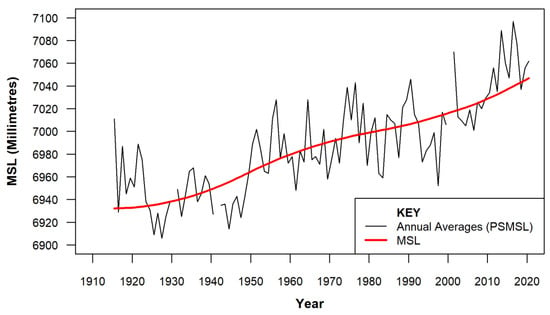
Figure 2.
Mean Sea Level (Fort Denison, Sydney). Refer Section 2.2 (Step 1) for more details.
Figure 3 summarises the hourly water level heights both above and below MSL over the same time frame, noting these measurements are the key artefact of interest for EVA. Some 903,659 hourly measurements spanning 105 years are available for analysis. The largest hourly water level height above MSL of +1456 mm was recorded on 25 May 1974 (1300 h) whilst the largest measurement below MSL of −1150 mm was recorded on 24 December 1999 (0600 h).
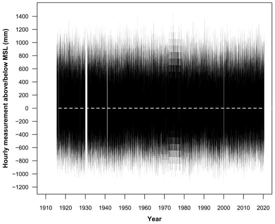
Figure 3.
Hourly measurements above and below MSL (Fort Denison, Sydney). Refer Section 2.2 (Step 2) for more details.
Table 2 summarises the largest hourly measurements above MSL determined from the analysis over the 105 years of hourly records available. Table 3 summarises the results of a linear regression analysis applied to the hourly measured water level above MSL across a range of cut-off heights to determine if there is any evidence of these extreme heights increasing (or decreasing) over time that might result from climate change (or other) influences. There is no evidence from the analysis that the slope of the linear regression of extreme heights against time are statistically different to zero (95% CI). The slope coefficient for the linear regression analyses for cut-off levels involving more than 100 data points are generally contained between ±0.3 mm/year. Only the analysis above a cut-off level of 900 mm above MSL indicates a slope statistically different to zero (95% CI) and the slope is negative, inferring a small lowering in the extreme measured heights above MSL over the record length.

Table 2.
Summary of Largest Hourly Measurements above MSL (>1280 mm).

Table 3.
Summary of Linear Regression Analysis for Hourly Measurements above MSL.
Figure 4 summarises the sensitivity analysis to select the optimum-fitted GPD for extreme value prediction, based on the four separate parameter optimisation approaches (i.e., MLE, GMLE, L-Moments, and Bayesian). Results are presented for threshold values ranging from 800 to 1200 mm based on analysis at 5 mm increments.
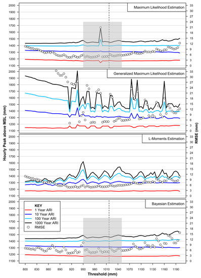
Figure 4.
Summary of sensitivity testing to optimise GPD model fit for EVA. Optimal model fitting denoted by grey shaded regions. Refer Section 2.2 (Step 4) for details. Vertical dashed line represents 99.7th percentile recommended by Arns et al. (2013) [27] for threshold setting.
The analysis clearly highlights the improved utility of the MLE and Bayesian approaches to GPD parameter optimisation for extreme value predictions using this data set. Both approaches exhibit consistency in prediction of extreme water levels across each return period depicted and across a wide range of thresholds. By contrast, the GMLE and L-Moments approaches prove overly sensitive to the threshold selection, in turn resulting in more erratic predictive capability with increasing return period (refer Figure 4, central panels), and therefore limited utility for robustly predicting extreme levels.
The key area of interest is denoted by the grey shaded regions in the top and bottom panels in Figure 4. The 99.7th percentile of hourly measurements (1017 mm) advocated by Arns et al. (2013) [27] as the optimal threshold setting, is denoted by vertical dashed lines for reference. These key areas of interest have been superimposed upon each other in Figure 5 to highlight key features.
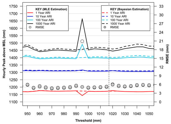
Figure 5.
Summary of optimal GPD model fitting range based on MLE and Bayesian approaches. Derived from Figure 4. Refer Section 2.2 (Step 4) for further details.
Firstly, from Figure 5, both the MLE and Bayesian approaches produce overwhelmingly consistent, robust predictive models for extreme value application, notably in the threshold range between 970 and 1015 mm as denoted by the lower RMSE’s.
The computationally expensive Bayesian approach, however, offers improved resilience against threshold sensitivity issues as evident from the anomalous MLE parameter optimisation approach at threshold 995 mm. Excluding this anomaly, the RMSE of the MLE is marginally improved by comparison to the Bayesian approach (≈3%).
The optimum-fitted GPD for estimating extreme water levels from the Fort Denison data set can be estimated via the MLE parameter fitting approach using a threshold set at 970 mm (which has the smallest RMSE at <4.6 mm). This visual summary of diagnostic analysis results enables sound EVA model fitting to confirm robust predictive capacity.
Table 4 summarises extreme hourly heights above MSL for a range of return periods using the optimum-fitted GPD function (Figure 6). The significant East Coast Low event in May 1974 dominates the extreme analysis with the recorded anomaly above MSL (1456 mm) estimated to have a return period exceeding 1000 years (1395). Such is the dominance of this event on the record, that the second and third highest hourly measurements (1396 and 1395 mm) recorded in 1956 and 1990, are estimated to have return periods of 100 and 97 years, respectively.

Table 4.
Predicted Extreme Hourly Height above MSL (Fort Denison, Sydney).
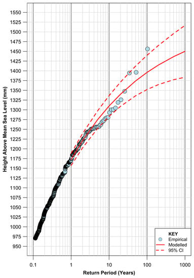
Figure 6.
EVA return periods for Fort Denison, Sydney. Based on optimal-fitted GPD model with parameters optimised using MLE approach and threshold level of 970 mm. Confidence intervals determined using a normal approximation approach provided by the extRemes package [31,32].
Table 5 provides a summary of estimated extreme hourly water levels for planning and design purposes over various planning horizons (2020, 2050, 2070, and 2100) incorporating sea level rise.

Table 5.
Predicted Extreme Hourly SWLs (Fort Denison, Sydney).
4. Discussion
Whilst employing state-of-the-art analytical techniques for MSL and extremes, this study gives rise to various discussion points, highlighted in the following sections.
4.1. Potential Future Changes to Storm Drivers That Could Influence Extreme Water Levels along the NSW Coast
The NSW coastline is affected by various storm typologies but East Coast Lows (ECLs), also known as east coast cyclones, are considered a dominant driver of climate for the region [44]. ECLs are driven by the temperature gradient between the Tasman Sea air and cold air in the high levels of the atmosphere over the continent and can produce gale to storm-force winds, coupled with very heavy rainfall [45]. ECLs are intense low-pressure systems that occur, on average, several times each year off the eastern coast of Australia, in particular southern Queensland and NSW [46].
The postulated climate change related influences on these weather systems, however, are not altogether clear. Although there is consensus from climate modelling on generally fewer ECLs occurring by the end of the century [46,47], some studies suggest that their intensity is also likely to weaken [46], whilst others suggest an increase in their intensity, and that these changes are strongest in spring and summer [47]. The lowering of atmospheric pressures during these events and potential increases to wind speeds (and therefore wave generating capacity) increases the likely storm surge characteristics under extreme conditions.
Tropical cyclones are a dominant and powerful storm system that features more prominently along the Queensland coastline generating over very warm tropical waters [45] where the sea surface temperature is greater than 26 °C [48,49]. They have relatively long-life cycles, typically about a week, and severe tropical cyclones (category 3 or greater) can produce wind speeds over 180 km/h near the centre, very heavy rainfall and large associated storm surges [45].
Laffoley and Baxter (2016) [50] indicate there is likely to be an increase in mean global ocean temperature of between 1 and 4 degrees Celsius by 2100. Under these conditions, tropical cyclones will be able to generate and migrate considerable distances further to the south to impact the NSW coastline more directly. The larger storm surges generated by these systems would, by consequence, increase the dynamic portion of extreme water levels experienced.
4.2. Sensitivity of EVA to Declustering
The application of GPD for POT EVA is underpinned by key assumptions of stationarity and independence. The stationarity protocol has been addressed through the removal of the MSL trend increasing over time (refer Section 2.2, Steps 1 and 2) and subsequent test results (refer Results and Table 3).
To satisfy statistical independence protocols between extreme events, the data must be carefully declustered. Following considerable sensitivity testing, Arns et al. (2013) [27] recommended that hourly tide gauge measurements used for EVA could satisfy independence requirements by setting a minimum of 25 h between separate extreme events. Figure 7 provides the results of sensitivity testing for extreme return periods, using three separate thresholds, by varying the delustering time between extreme events from 0 to 100 h. Similar to the results of Arns et al. (2013) [27], there is limited influence on the predicted extreme return periods once the time between successive extreme peaks increases to 25 h. This is to be expected with the lunar day being 24 h and 50 min; thus, by setting the declustering limit between peaks to at least 25 h, successive tidal peaks will be considered within the same extreme event, which is a key consideration when extreme events coincide with high spring tidal phenomena. When the declustering of events is set at a threshold less than 25 h, successive large tidal peaks which form a significant portion of the peak water level for the same extreme event will be considered separate extreme events, violating the independence assumptions underpinning GPD and POT theory.
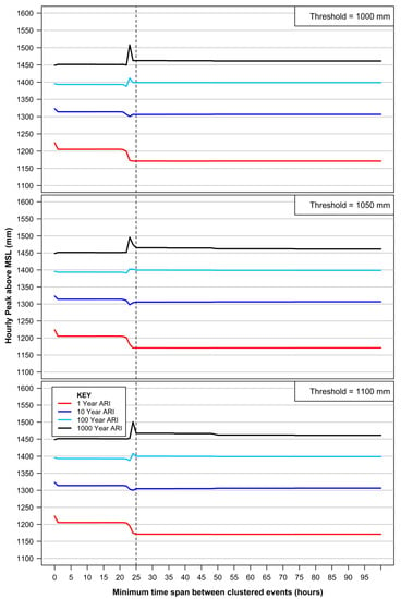
Figure 7.
Sensitivity analysis for declustering time spans. The vertical dashed line at 25 h represents the minimum hourly time frame to decluster events.
4.3. Sensitivity of EVA to Length of Dataset
It is important to understand the limitations of any EVA without diminishing the obvious utility of providing scientifically derived estimates of natural phenomena that often lie beyond the physical time scale of measurements experienced to date. In this regard, the long hourly time series of measurements extending from 1915 to 2020 provide the means to test the importance of both the length of the data set and dominant measured events contained within.
Figure 8 summarises outputs from one-third portions of the data set (1915–1950, 1950–1985, 1985–2020) compared to the full data set (1915–2020) and the full data set with the exclusion of the 1974 event which dominates the record. Using the full data set and excluding the 3 hourly water levels measured around the peak of the event on 25 May 1974 reduces the predicted hourly peak above MSL for 10, 100, and 1000-year return period events by some 12 mm (1%), 28 mm (2%), and 42 mm (3%), respectively. This analysis provides some guide to the sensitivity of the results to such a pivotal event on the record, noting it is not uncommon for measurement system malfunction during very extreme natural events.
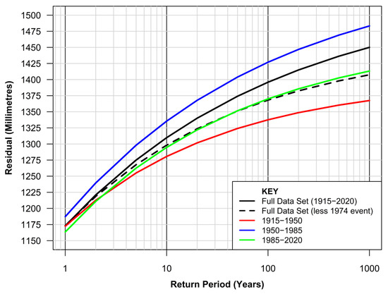
Figure 8.
Sensitivity analysis on length of data set for EVA (Fort Denison, Sydney).
However, as might be expected from EVA, the results are more critically affected by the length of the dataset available. Analysis of the three 35-year portions of the full dataset increases the sensitivity of the predicted hourly peak above MSL for 10, 100 and 1000-year return period events by a maximum of 29 mm (2.2%), 58 mm (4.2%) and 82 mm (5.7%), respectively, compared to the results from the full data set.
These differences are put into some perspective when one considers only 54 mm distinguishes between the 100 and 1000-year return period extreme water level for the optimally fitted GPD for the full data set.
4.4. Threshold Selection and GPD Fitting for POT Analysis
Based on sensitivity testing, Arns et al. (2013) [27] provided a range of recommendations for EVA using hourly tide gauge records, including setting the threshold for POT analysis at the 99.7th percentile of hourly measurements and optimizing the selection of parameters for GPD fitting using an MLE approach. The determination of the optimal threshold level to adopt when applying the POT approach dominates much of the contemporary literature around EVA. The testing and selection approach by Arns et al. (2013) [27] to recommend use of the 99.7th percentile of hourly measurements was based on a rational desire to seek a less subjective approach. However, the approach advocated in this paper to consider various key metrics, graphically represented across a range of thresholds and parameter optimisation approaches (Figure 4 and Figure 5), provides a more robust and objective methodology given any overly sensitive artefacts of parameter optimisation fitting are immediately apparent (and therefore avoided). This is enhanced by the ready availability of diagnostic tools available in modern EVA software. It is acknowledged in this case that the selection of the of 99.7th percentile of hourly measurements (1017.1 mm) would have resulted in a near identical outcome for the model fit and predicted extreme values (refer Table 6), only that the RMSE for the model fit improves slightly from 5.46 mm to 4.59 mm for the threshold of 970 mm adopted in this study.

Table 6.
Comparison of Predicted Extreme Hourly Height above MSL.
4.5. Spatial Utility of EVA
The EVA results advised are a combination of predictable tidal behaviours and a wide variety of largely unrelated dynamic oceanographic effects occurring over differing timescales from high intensity, short duration storm surges to longer timescale climate mode influences (such as ENSO). Whilst the high frequency hourly water levels will have a distinct spatial signature based on dominant regional scale storm patterns, the more predictable tidal characteristics are also spatially dependent. Whilst the tidal range increases marginally from south to north along the NSW coastline (≈200 mm), the largest offshore wave statistics are evident from measured data at the Sydney and Port Kembla waverider buoy systems [51], both of which are situated within 80 km of the Fort Denison tide gauge.
Similarly, the dominance of the 1974 storm event which had its greatest impacts across the Greater Metropolitan Region of Sydney were captured in the Fort Denison tide gauge record. This record is unique in NSW both due to its length (dating back to 1915) and in the fact it captured the full 1974 event. Sensitivity analyses (see Section 4.3) highlight the importance of longer records and capturing rare events for improving the prediction capability of high frequency extremes. Therefore, the results of the EVA of the Fort Denison record are considered to represent a very good proxy for high frequency extremes along the NSW coastline for both planning and design purposes.
5. Conclusions
The extensive hourly data repository of measured water levels at Fort Denison dating back to 1915 provide the basis to consider both high frequency extreme water levels and low frequency sea level rise at Sydney. This analysis also integrates recent updated IPCC projections of sea level rise to 2100 [3], providing sea level extremes for a range of return periods over future planning horizons for design, planning, and sea level adaptation purposes that are relevant for application along the NSW coastline (refer Table 5).
The largest measured height above MSL at Fort Denson of +1456 mm was recorded on 25 May 1974 (1300 h) during an extreme ECL event which resulted in considerable damage within the Greater Metropolitan Region of Sydney and adjacent coastlines. From the EVA undertaken, this height above MSL is estimated to have a return period of 1395 years. The next highest measured extremes in 1956 and 1990, respectively (1396 and 1395 mm) have an estimated return period of ≈100 years. The sensitivity of the extreme tail of the fitted GPD is clear with a rise of ≈60 mm increasing the return period from 100 to almost 1400 years.
In this regard, it is important to note that, up until 1999, hourly data at Fort Denison was recorded only to the nearest centimetre. In addition, the estimate of MSL at each of these respective years has an estimated 95% confidence level of just under ±10 mm, highlighting the key sensitivity that measurement accuracy might play in estimating extreme return periods at the rare end of the Fort Denison dataset.
The analysis also provides no evidence (at the 95% CI) at this point in time that extreme measured water levels above MSL have been increasing over time at Fort Denison due to climate change (or any other factors).
The analysis permits an understanding of the influence that slow and incremental sea level rise plays on the nature of extreme projections for oceanic inundation risk. Considering the amount of sea level rise estimated at Fort Denison between 1974 and 2020 (≈52 mm), a peak hourly height above MSL of 1404 mm in 2020 would be required to reach the same measured water level as the peak in 1974, which has an order of magnitude reduction in return period to ≈132 years (cf. 1395 years in 1974). Taking this a step further, if one considers the amount of sea level rise forecast between 2020 and 2050 under a high sea level rise scenario (i.e., SSP5-8.5, 180 mm), the extreme hourly height above MSL required in 2050 to reach the same level as the devastating event in 1974, would be occurring on average every 2 years. These relatively simple statistical comparisons serve to highlight the ongoing and increasing threat of oceanic inundation posed by rising MSL.
The analysis is based on a POT approach and optimised fitting of the GPD to predict extreme values following the recommendations advocated by Arns et al. (2013) [27], but with two suggested improvements. Firstly, the estimate of MSL used to de-trend the hourly tide gauge data is based on more recent advancements in this area, and secondly, this study recommends the use of a slightly improved diagnostic approach to selection and optimisation of an appropriate threshold above which the EVA is performed. The fitted GPD results in a low RMSE of <4.6 mm, providing some assurance in the utility of this tool to predict hourly extremes above MSL from the Fort Denison measured data.
The analytical procedures described provide a step-by-step guide for practitioners on how to develop similar baseline information from any long tide gauge record and the associated limitations and key sensitivities that must be understood and appreciated in doing so. The analysis and results presented in this paper provide a very good resource for coastal zone management, design, and sea level rise adaptation planning along the NSW coastline.
Funding
This research received no external funding.
Institutional Review Board Statement
Not applicable.
Informed Consent Statement
Not applicable.
Data Availability Statement
Data set available on request to corresponding authors.
Acknowledgments
The author would like to thank the following: Ivan Haigh (Ocean and Earth Science, National Oceanography Centre, University of Southampton, UK) for reviewing and providing suggestions to improve the draft manuscript; John Hunter (University Associate, University of Tasmania, Australia) for reviewing and providing suggestions to improve the draft manuscript; Eric Gilleland (Research Applications Laboratory, National Center for Atmospheric Research, University Corporation for Atmospheric Research, Boulder, CO, USA) for discussions on EVA and application of ‘extRemes’ software package; National Operations Centre (NOC) Tidal Unit, Australian Bureau of Meteorology for access to hourly Fort Denison data spanning 1914 to 1994; University of Hawaii, Sea Level Centre for their publicly accessible data repository of hourly tide gauge measurements; and Permanent Service for Mean Sea Level for their publicly accessible data repository.
Conflicts of Interest
The author declares no conflict of interest.
References
- Steffen, W.; Mallon, K.; Kompas, T.; Dean, A.; Rice, M. Compound Costs: How Climate Change Is Damaging Australia’s Economy; Climate Council of Australia: Potts Point, Australia, 2019; ISBN 978-1-925573-97-8. [Google Scholar]
- Nauels, A.; Gütschow, J.; Mengel, M.; Meinshausen, M.; Clark, P.U.; Schleussner, C.-F. Attributing long-term sea-level rise to Paris Agreement emission pledges. Proc. Natl. Acad. Sci. USA 2019, 116, 23487–23492. [Google Scholar] [CrossRef] [PubMed]
- IPCC; Masson-Delmotte, V.; Zhai, P.; Pirani, A.; Connors, S.L.; Péan, C.; Berger, S.; Caud, N.; Chen, Y.; Goldfarb, L.; et al. Climate Change 2021: The Physical Science Basis. Contribution of Working Group I to the Sixth Assessment Report of the Intergovernmental Panel on Climate Change. 2021. Available online: https://elib.dlr.de/137584/ (accessed on 21 September 2021).
- Watson, P.J. Status of mean sea level rise around the USA (2020). GeoHazards 2021, 2, 80–100. [Google Scholar] [CrossRef]
- Woodworth, P.L.; Hunter, J.R.; Marcos, M.; Caldwell, P.; Menéndez, M.; Haigh, I. Towards a global higher-frequency sea level dataset. Geosci. Data J. 2016, 3, 50–59. [Google Scholar] [CrossRef]
- Modra, B. NSW Ocean Water Levels; Report No. MHL1881; Technical Report Prepared by Public Works Manly Hydraulics Laboratory; NSW Government: Sydney, Australia, March 2011.
- Queensland Government. Tropical Cyclone Yasi February 2011. Report from Department of Environment and Resource Management, Queensland Government. 2011. Available online: https://www.publications.qld.gov.au/dataset/19c20822-f29e-494c-880a-113ccd13a04b/resource/3bf0ac2c-565a-4400-8d5b-6a4c15236c82/download/tc-yasi.pdf (accessed on 21 September 2021).
- Rashid, M.M.; Wahl, T.; Chambers, D.P. Extreme sea level variability dominates coastal flood risk changes at decadal time scales. Environ. Res. Lett. 2021, 16, 024026. [Google Scholar] [CrossRef]
- Thompson, P.R.; Widlansky, M.J.; Hamlington, B.D.; Merrifield, M.A.; Marra, J.J.; Mitchum, G.T.; Sweet, W. Rapid increases and extreme months in projections of United States high-tide flooding. Nat. Clim. Chang. 2021, 11, 584–590. [Google Scholar] [CrossRef]
- Hague, B.S.; McGregor, S.; Murphy, B.F.; Reef, R.; Jones, D.A. Sea level rise driving increasingly predictable coastal inundation in Sydney, Australia. Earth’s Future 2020, 8, e2020EF001607. [Google Scholar] [CrossRef]
- Pattiaratchi, C.; Wijeratne, E.M.S. Observations of Meteorological Tsunamis along the South-West Australian Coast. Nat. Hazards 2014, 74, 281–303. [Google Scholar] [CrossRef][Green Version]
- Ozsoy, O.; Haigh, I.D.; Wadey, M.P.; Nicholls, R.J.; Wells, N.C. High-frequency sea level variations and implications for coastal flooding: A case study of the Solent, UK. Cont. Shelf Res. 2016, 122, 1–13. [Google Scholar] [CrossRef]
- Tebaldi, C.; Ranasinghe, R.; Vousdoukas, M.; Rasmussen, D.J.; Vega-Westhoff, B.; Kirezci, E.; Kopp, R.E.; Sriver, R.; Mentaschi, L. Extreme sea levels at different global warming levels. Nat. Clim. Chang. 2021, 11, 746–751. [Google Scholar] [CrossRef]
- Buchanan, M.K.; Oppenheimer, M.; Kopp, R.E. Amplification of flood frequencies with local sea level rise and emerging flood regimes. Environ. Res. Lett. 2017, 12, 064009. [Google Scholar] [CrossRef]
- Fréchet, M. On the law of probability of the maximum deviation. Ann. Pol. Math. Soc. 1927, 6, 93–116. [Google Scholar]
- Fisher, R.A.; Tippett, L.H.C. Limiting forms of the frequency distribution of the largest or smallest member of a sample. Math. Proc. Camb. Philos. Soc. 1928, 24, 180–190. [Google Scholar] [CrossRef]
- Gumbel, E.J. The maxima of the mean largest value and of the range. Ann. Math. Stat. 1954, 25, 76–84. [Google Scholar] [CrossRef]
- Weibull, W. A statistical distribution function of wide applicability. J. Appl. Mech. 1951, 18, 293–297. [Google Scholar] [CrossRef]
- Jenkinson, A.F. The frequency distribution of the annual maximum (or minimum) values of meteorological elements. Q. J. R. Meteorol. Soc. 1955, 81, 158–171. [Google Scholar] [CrossRef]
- Coles, S. An Introduction to Statistical Modeling of Extreme Values; Springer: London, UK, 2001; ISBN 978-1-84996-874-4. [Google Scholar]
- Pickands, J. The two-dimensional poisson process and extremal processes. J. Appl. Probab. 1971, 8, 745–756. [Google Scholar] [CrossRef]
- Pickands, J. Statistical inference using extreme order statistics. Ann. Stat. 1975, 3, 119–131. [Google Scholar]
- Beirlant, J.; Goegebeur, Y.; Teugels, J.; Segers, J. Statistics of Extremes; John Wiley & Sons, Ltd.: Chichester, UK, 2004; ISBN 9780470012383. [Google Scholar]
- Shane, R.M.; Lynn, W.R. Mathematical model for flood risk evaluation. J. Hydraul. Div. 1964, 90, 1–20. [Google Scholar] [CrossRef]
- Charras-Garrido, M.; Lezaud, P. Extreme value analysis: An introduction. J. Société Française Stat. Rev. Stat. Appliquée 2013, 154, 66–97. [Google Scholar]
- Dupuis, D.J. Exceedances over high thresholds: A guide to threshold selection. Extremes 1999, 1, 251–261. [Google Scholar] [CrossRef]
- Arns, A.; Wahl, T.; Haigh, I.D.; Jensen, J.; Pattiaratchi, C. Estimating extreme water level probabilities: A comparison of the direct methods and recommendations for best practise. Coast. Eng. 2013, 81, 51–66. [Google Scholar] [CrossRef]
- Caires, S. Extreme Value Analysis: Wave Data; JCOMM Technical Report; WMO: Geneva, Switzerland, 2011. [Google Scholar]
- Watson, P.J. Improved Techniques to Estimate Mean Sea Level, Velocity and Acceleration from Long Ocean Water Level Time Series to Augment Sea Level (and Climate Change) Research; University of New South Wales: Sydney, Australia, 2018. [Google Scholar]
- R Development Core Team R. A Language and Environment for Statistical Computing; R Foundation for Statistical Computing: Vienna, Austria, 2021. [Google Scholar]
- Gilleland, E. ExtRemes: Extreme Value Analysis; R Foundation for Statistical Computing: Vienna, Austria, 2021. [Google Scholar]
- Gilleland, E.; Katz, R.W. ExtRemes 2.0: An extreme value analysis package in R. J. Stat. Softw. 2016, 72, 1–39. [Google Scholar] [CrossRef]
- PSMSL. Permanent Service for Mean Sea Level. Available online: https://www.psmsl.org/data/obtaining (accessed on 21 September 2021).
- Holgate, S.J.; Matthews, A.; Woodworth, P.L.; Rickards, L.J.; Tamisiea, M.E.; Bradshaw, E.; Foden, P.R.; Gordon, K.M.; Jevrejeva, S.; Pugh, J. New data systems and products at the permanent service for mean sea level. J. Coast. Res. 2013, 29, 493–504. [Google Scholar] [CrossRef]
- UHSLC. University of Hawaii Sea Level Centre. Available online: http://uhslc.soest.hawaii.edu/data (accessed on 22 September 2021).
- Caldwell, P.C.; Merrifield, M.A.; Thompson, P.R. Sea Level Measured by Tide Gauges from Global Oceans—The Joint Archive for Sea Level Holdings (JASL); NOAA National Centers for Environmental Information: Asheville, NC, USA, 2001.
- Watson, P.J. Identifying the Best Performing Time Series Analytics for Sea Level Research. In Time Series Analysis and Forecasting: Contributions to Statistics; Rojas, I., Pomares, H., Eds.; Springer International Publishing: Cham, Switzerland, 2016; pp. 261–278. [Google Scholar]
- Watson, P.J.; Lim, H.S. An update on the status of mean sea level rise around the Korean peninsula. Atmosphere 2020, 11, 1153. [Google Scholar] [CrossRef]
- Kondrashov, D.; Ghil, M. Spatio-temporal filling of missing points in geophysical data sets. Nonlinear Processes Geophys. 2006, 13, 151–159. [Google Scholar] [CrossRef]
- Alexandrov, T.; Golyandina, N. Automatic Extraction and Forecast of Time Series Cyclic Components within the Framework of SSA. In Proceedings of the 5th St. Petersburg Workshop on Simulation, St. Petersburg, Russia, 26 June–2 July 2005; pp. 45–50. [Google Scholar]
- Mann, M.E.; Steinman, B.A.; Miller, S.K. Absence of internal multidecadal and interdecadal oscillations in climate model simulations. Nat. Commun. 2020, 11, 49. [Google Scholar] [CrossRef]
- Katz, R.W.; Parlange, M.B.; Naveau, P. Statistics of extremes in hydrology. Adv. Water Resour. 2002, 25, 1287–1304. [Google Scholar] [CrossRef]
- IPCC. Summary for Policymakers. In Climate Change 2021: The Physical Science Basis. Contribution of Working Group I to the Sixth Assessment Report of the Intergovernmental Panel on Climate Change; Masson-Delmotte, V., Zhai, P., Pirani, A., Connors, S.L., Péan, C., Berger, S., Caud, N., Chen, Y., Goldfarb, L., Gomis, M.I., et al., Eds.; Cambridge University Press: Cambridge, UK, 2021. [Google Scholar]
- Dowdy, A.J.; Mills, G.A.; Timbal, B. Large-Scale Indicators of Australian East Coast Lows and Associated Extreme Weather Events; CAWCR Technical Report No. 037; Centre for Australian Weather and Climate Research: Aspendale, Australia, 2011. [Google Scholar]
- Australian Government, Bureau of Meteorology. About East Coast Lows. Available online: http://www.bom.gov.au/nsw/sevwx/facts/ecl.shtml (accessed on 21 September 2021).
- Ji, F.; Evans, J.P.; Argueso, D.; Fita, L.; di Luca, A. Using large-scale diagnostic quantities to investigate change in east coast lows. Clim. Dyn. 2015, 45, 2443–2445. [Google Scholar] [CrossRef]
- Grose, M.R.; Pook, M.J.; McIntosh, P.C.; Risbey, J.S.; Bindoff, N.L. The simulation of cutoff lows in a regional climate model: Reliability and future trends. Clim. Dyn. 2012, 39, 445–459. [Google Scholar] [CrossRef]
- Palmen, E. On the formation and structure of tropical hurricanes. Geophysica 1948, 3, 26–38. [Google Scholar]
- Dare, R.A.; Mcbride, J.L. The threshold sea surface temperature condition for tropical cyclogenesis. J. Clim. 2011, 24, 4570–4576. [Google Scholar] [CrossRef]
- Laffoley, D.; Baxter, J.M. (Eds.) Explaining Ocean Warming: Causes, Scale, Effects and Consequences; Full Report; International Union for Conservation of Nature: Gland, Switzerland, 2016; 456p. [Google Scholar] [CrossRef]
- MHL. Manly Hydraulics Laboratory. Available online: https://www.mhl.nsw.gov.au/Data-Wave (accessed on 30 September 2021).
Publisher’s Note: MDPI stays neutral with regard to jurisdictional claims in published maps and institutional affiliations. |
© 2022 by the author. Licensee MDPI, Basel, Switzerland. This article is an open access article distributed under the terms and conditions of the Creative Commons Attribution (CC BY) license (https://creativecommons.org/licenses/by/4.0/).


