Abstract
This paper studied the chemical characteristics and seasonal changes of PM2.5 in plateau cities on the southwest border of China. Urban air was sampled in Baoshan City during the rainy and dry seasons. Finally, 174 PM2.5 filters were collected (including 87 quartz and 87 Teflon samples for PM2.5). The mass concentrations, water-soluble inorganic ions, organic and inorganic carbon concentrations, and inorganic elements constituting PM2.5 were determined. Positive definite matrix factorization was used to identify potential sources of PM2.5, and the backward trajectory model was used to calculate the contribution of the long-distance transmission of air particles to the Baoshan area. It was found that in the wet season, most of the air masses come from the Indian Ocean and Myanmar. In the dry season, the air mass mainly comes from the China and Myanmar border area. The average concentration of PM2.5 in the wet and dry seasons was 23.17 ± 12.23 μg/m3. The daily mean value of OC/EC indicated that the measured SOC content was generated by the photochemical processes active during the sampling days. However, elements from anthropogenic sources (Na, Mg, Al, Si, P, K, Ca, Ti, Fe, Cu, Zn, Sb, Ba, and Pb) accounted for 99.51% and 99.40% of the total inorganic elements in the wet season and dry season, respectively. Finally, source apportionment showed that SIA, dust, industry, biomass burning, motor vehicle emissions, and copper smelting emissions constituted the major contributions of PM2.5 in Baoshan. Using combined data from three measurement sites provides a focus on the common sources affecting all locations.
1. Introduction
In recent decades, with rapid economic development, industrialization, and urbanization in China, the number of motor vehicles and the total energy consumption has increased. As a result, atmospheric particulate matter (PM) has become one of the most significant air contaminants [1,2,3]. PM2.5 (aerodynamic diameter ≤ 2.5 μm) can exist in the atmosphere for a long time, conducive to its long-distance transport through the atmosphere and deposition towards remote areas. During long-range transport, PM2.5 carries abundant anthropogenic pollutants. It has a serious impact on the global and regional climate, the visibility and composition of the atmosphere, the global biogeochemical cycles, and the activation of cloud condensation nuclei [4,5,6].
In recent years, PM2.5 has been widely studied in China due to its potential impacts on air quality and human health. Water-soluble inorganic ions (WSIIs), organic carbon (OC) particles, inorganic carbon (EC) particles, and inorganic elements (IEs), the main chemical components of PM2.5, have been extensively studied in China [7,8,9]. WSIIs are dominated by secondary inorganic aerosols (SIAs), including NH4+, NO3−, and SO42−. OC is composed of thousands of organic compounds and contains many toxic substances. An important part of the inorganic elements of PM2.5 are heavy metals, such as Fe, Cu, Zn, and Pb [10,11,12].
Whether worldwide or only in China, it is essential to reduce PM2.5 concentrations to control their sources. The key point in formulating policies for the government to control PM2.5 pollution is the result of source apportionment and reliable source quantification [13,14].PM2.5 is usually sourced by the emission of pollutants, and its classification is very complex, including its anthropogenic and natural sources and gas and particle phases [15,16]. In addition, PM2.5 forms secondary pollutants from primary emissions through photochemical reactions after being released from pollution sources, making it difficult to quantify its impacts [17,18,19]. The contribution levels of different sources in the air can be quantitatively estimated using the receptor model. Generally, researchers have found the possible sources of PM2.5 as traffic and industrial, coal combustion, biomass burning, and secondary inorganic aerosol sources [20,21].
In recent years, most studies have generally focused on the Jing-Jin-Ji region and its coastal areas with severely degraded atmospheric environments in China [22,23,24]. Only a few researchers have investigated PM2.5 pollution in Yunnan Province, a remote southwestern region. More research has been conducted in areas such as Kunming and Yuxi [25,26,27]. Despite the economic backwardness of the remote southwestern mountains, there are still cases of PM2.5 exceeding the standard every year [28,29,30]. More and more people have begun to study cross-border pollution. More often, air pollution comes not only from the locals but also from the pollution emissions of surrounding areas. This paper aims to study the source distribution of PM2.5 in Baoshan, the southwest border of China, and explore the impact of China’s surrounding countries on the climate of Baoshan City. By studying the distribution of local air pollution sources and reasonably evaluating the distribution of cross-border pollution and local air pollution sources, it is not only of great significance for the local government to formulate prevention and control countermeasures but also of great guiding significance for interregional cooperation. Therefore, we should pay more attention to these areas to improve overall air quality.
PM2.5 samples were collected in the wet and dry seasons at three monitoring sites of the urban area of Baoshan. The concentrations of PM2.5, WSII, OC, EC, and IEs were analyzed and discussed in this study. Positive definite matrix factorization (PMF) was used for source apportionment of PM2.5 to analyze pollution sources. Potential major contributors were identified based on PMF and local environmental background information. The details of PM2.5 pollution characteristics and source allocation results in this study can provide reasonable and effective measures for local governments to slow down PM2.5 air pollution.
2. Methods
2.1. Sampling Site and Sample Collection
Baoshan is a developing industrialized city with 1 million residents and an urban area of 149.9 km2. In 2016, the coal consumption of Baoshan was 983,900 tons, and the region housed approximately 200,000 motor vehicles. Baoshan is located in the west of Yunnan Province, which is close to Myanmar, between 95°25′–10°02′ E and 24°08′–25°51′ N.
Baoshan is located at the southern end of the longitudinal valley in western Yunnan of the Hengduan Mountains. The terrain is complex and diverse. The dam area accounts for 8.21%, and the mountainous area accounts for 91.79%. The whole terrain extends and tilts from northwest to southeast. The lowest altitude is 535 m, the highest altitude is 3780.9 m, and the average altitude is about 1800 m. Baoshan has a low latitude mountain subtropical monsoon climate. As the region is located in a low latitude plateau, the landform is complex. There are seven climate types: north tropical, south subtropical, middle subtropical, north subtropical, south temperate, middle temperate, and plateau climate. It is characterized by a small annual temperature difference and a large daily temperature difference; the rainfall is abundant, dry, and wet, with annual rainfall of 700–2100 mm.
The airflow near the ground can only enter the urban area from the southeast. The cold air in Siberia from the north is blocked by the mountains. The monsoon in the Beibu Gulf and the Bay of Bengal flows from the southeast to the urban area, forming comfortable temperatures, low wind speeds, and high ultraviolet (UV) lighting conditions throughout the year. Strong ultraviolet light is conducive to the formation of photochemical atmospheric effects. Under the conditions of low pressure and low oxygen, this can lead to the incomplete combustion of fuel, thus increasing the resulting pollution emissions. When the wind speed is low (<3 m/s) and the temperature changes greatly between day and night, it is easy to form an inversion layer, which hinders the diffusion of pollutants.
Measurement campaigns of PM2.5 sampling at three sites at the Baoshan College (BSC), Athlete apartment (AA), and Environmental Monitoring Station of Baoshan (EMS) in Baoshan city (Figure 1), were carried out in two periods in 2016, i.e., 13 June to 27 June and 9 November to 23 November. According to the 2016 annual data of Baoshan city form China Weather Network (http://www.weather.com.cn), (accessed on 10 October 2021) found that Baoshan experienced abundant precipitation in June but little rainfall in the November dry climate. Therefore, this paper presents June as the wet season and November as the dry season. Daily measurements of 22 ± 1 h with an intelligent mid-volume atmospheric particulate sampler (TH-150F, Tianhong, Wuhan, China) were conducted at a 100 L/min sample flow. Teflon filters (Wuhan, China, 90 mm) were used to analyze IEs, and quartz filters (PALL Inc., New York City, NY, USA, 90 mm) were used to analyze OC, EC, and WSIIs. A total of 174 PM2.5 samples and 12 blank samples were collected. After sampling, the filters were individually placed into plastic boxes and put into a freezer at −20 °C until transport and subsequent analysis. The attached Table S1 lists the weather conditions during the sampling period.
Figure 1.
Location of the sampling sites in Baoshan, China.
2.2. Chemical Analysis and Quality Control
2.2.1. WSII Analysis
The anion (i.e., F−, Cl−, SO42−, and NO3−) and cation (i.e., K+, Ca2+, Mg2+ and NH4+) concentrations were measured by ion chromatography (DX-600, Dionex, Sunnyvale, CA, USA). This system was outfitted with a separation column (Dionex AS-14A for anions and CS-12A for cations) and a guard column (Dionex AG14A for anions and CG12A for cations). A gradient weak base eluent (3.5 mmol/L Na2CO3; 1 mmol/L NaHCO3) was used for anion detection, while a weak acid eluent (18 mmol/L methanesulfonic acid) was used for cation detection. The measurement error of each ion in a standard solution was within 10%, and the average relative standard deviations of anions and cations are 3.0% and 4.0%, respectively. For quality assurance, two blank spaces were detected in each batch of samples, and the test was carried out at 10%. At least six standard solution concentrations needed to be mixed for each ion component.
2.2.2. Elements Analysis
Li, Be, P, Sc, V, Cr, Mn, Co, Ni, Cu, As, Rb, Sr, Zr, Mo, Sn, Sb, Cs, La, Ce, Sm, W, Pb, Bi, Th, and U were analyzed by inductively coupled plasma-mass spectrometry (ICP-MS). Na, Mg, Al, Si, K, Ca, Ti, Fe, Zn, and Ba were analyzed by inductively coupled plasma-atomic emission spectrometry (ICP-AES). The instrument was calibrated with reference materials to make the measurement results as accurate as possible. For quality assurance and quality control (QA/QC), the same procedures were used for the pretreatment and analysis of standard reference materials, and the recovery values of all target elements were within the range of certified values or within 5% of certified values.
2.2.3. OC and EC Analysis
OC and EC were analyzed using the DRI Model 2001 OC/EC Analyser, which was developed by the American Desert Institute (DRI). The main testing principle of this method is as follows: the sample was heated and converted into CO2 under different temperature gradients and gas environments. CO2 was reduced to CH4 by catalyzing MnO2 and was detected using a flame ion detector (FID). Then, using a 633 nm helium/neon laser to detect the anti-light intensity of filter paper to detect the production of organic pyrolysis carbon (OPC), eight different carbon components (OC1, OC2, OC3, OC4, OPC, EC1, EC2, and EC2) were obtained. IMPROVE (Interagency Monitoring of Protected Visual Environments) defined OC as OC1 + OC2 + OC3 + OC4 + OCPyro and EC as EC1 + EC2 + EC3-OCPyro. The detection limits were 0.82 (OC), 0.19 (EC), and 0.93 (TC) μg/cm2, and the measuring range was 0.2~750 μg/cm2.
2.2.4. Quality Assurance and Control
The quartz filters were baked at 450 ℃ for 5 h in a muffle furnace before sampling to identify the possible presence of organics. All filters were placed in a clean room (temperature of 25 ± 5 ℃; relative humidity of 50 ± 5%) for 48 h and weighed by a high-precision electronic balance (EX125ZH) with an accuracy of 10 μg before and after sampling. Each filter was weighed twice, with the difference between the two results not exceeding 10 μg for quartz filters and Teflon filters to guarantee the precision of the weighing results. All filters were stored in a freezer at −20 °C before analysis to prevent the loss of volatile components.
In the sample analysis process, the instrument was calibrated with standard gas before and after the sample analysis. Then, one sample was randomly selected from every 10 samples for parallel analysis, and the standard sample was measured twice a week. The recovery rate of the standard sample was 98–102%. Finally, the system blank of the instrument and the blank of the laboratory system were measured every week. The results showed no contamination during sample handling and collection, as assured by the quality assurance and control (QC/QA) procedures.
2.3. Data Processing
2.3.1. Positive Definite Matrix Factorization (PMF) Modeling
The source apportionment of PM2.5 was carried out through the PMF 5.0 model of the U.S. Environmental Protection Agency. PMF is a quantitative receptor source analytical model based on the least square method [31,32]. As one of the most successful receptor models, it divides the sample data into two matrices, namely, the source component spectrum matrix F(k × j) and source contribution matrix G(I × k) [33,34]. The formula can be expressed where is the concentration of the j-th species in the i-th sample, is the contribution of the k-th factor to the i-th sample, is the species fraction of the j-th species from the k-th source, eij is the residue related to the concentration of the j-th species measured in the i-th sample, and P represents the total number of pollution sources.
The objective function Q can check the allocation of each species so as to evaluate the accuracy of the model.
Among is the uncertainty of the j-th species in the i-th sample.
The uncertainty of data will affect the PMF results, and the measurement uncertainty is the input parameter of the PMF analysis [35]. At the same time, the operation of other auxiliary equations can also be added to make the source allocation operation more reasonable. The auxiliary equation can be applied to the selected solution in the form of constraints, which will rotate the solution and make the results more meaningful. In addition, some non-zero rotations can be introduced into the matrix to improve the rotation stability of the solution [36]. We assume that each sampling site has pollution contributions from similar sources. For example, although the contribution proportion of traffic sources at suburban sites is smaller than that at urban sites, both sites have similar pollution sources. Based on this assumption, we combined the data of three points. Thus, the sample size of the PMF model was increased. After merging the data, the PMF source results may pay more attention to general phenomena rather than special local changes [37].
2.3.2. HYSPLIT4 Model
The HYSPLIT4 model is a professional model jointly developed by the National Oceanic and Atmospheric Administration Air Resources Laboratory and the Australian Bureau of Meteorology in the past 20 years to calculate and analyze the transport and diffusion trajectories of atmospheric pollutants. The model has a relatively complete transport, diffusion, and sedimentation model that can handle multiple meteorological element input fields, multiple physical processes, and different types of pollutant emission sources. This model is widely used in the study of the transmission and diffusion of multiple pollutants in various regions. In this study, the independent version of the backward trajectory model was used, the auxiliary software package was used (GUI; Ghostscript; Image Magick, Landenberg, PA, USA), and the meteorological data were obtained through NCEP (National Centers for Environmental Prediction) and GDAS (Global Data Assimilation System).
3. Results and Analyses
3.1. Characteristics of PM2.5
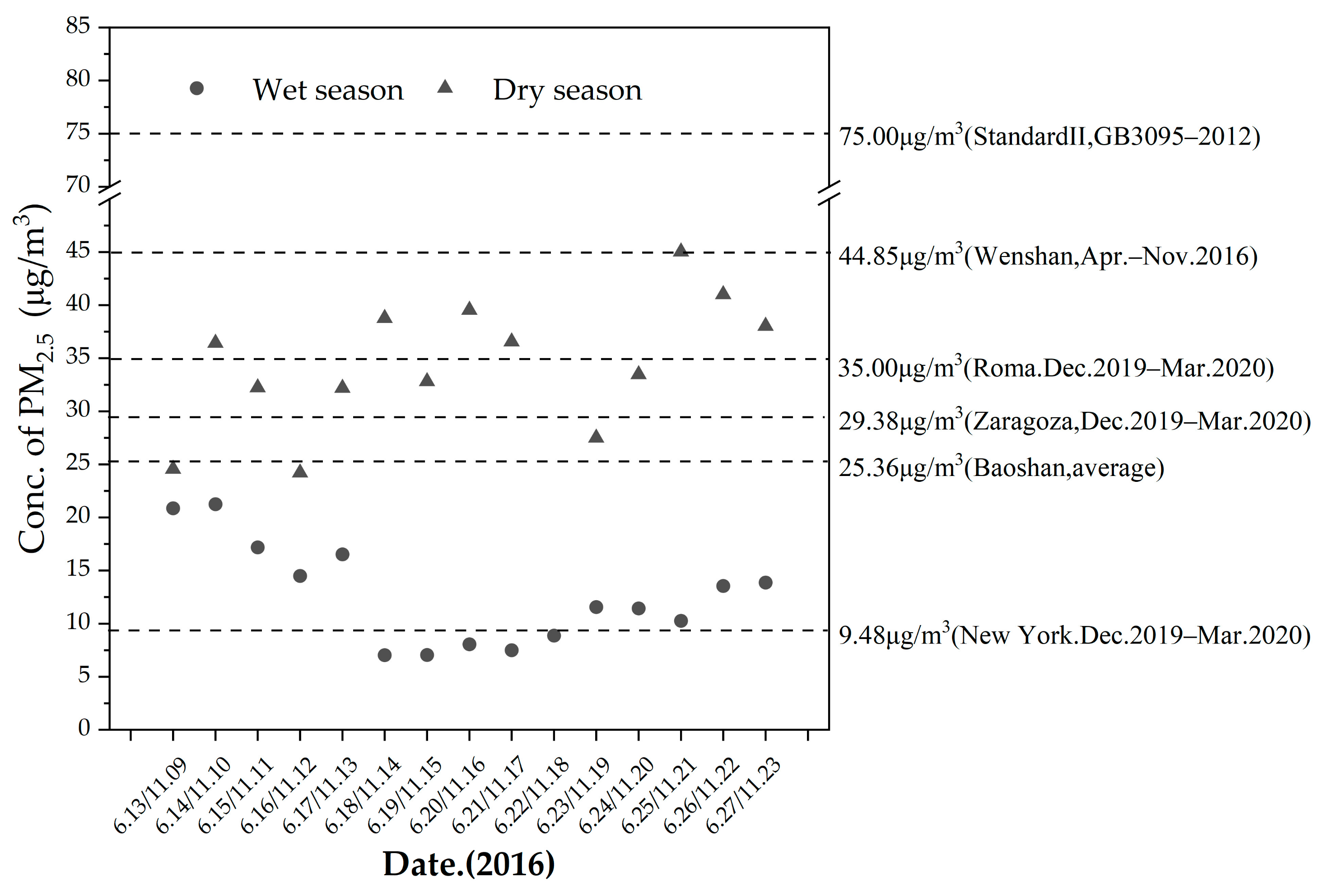
During the two sampling campaigns, the mass concentrations (from Telfon filters) of PM2.5 ranged from 7.03 μg/m3 to 21.24 μg/m3 in the wet season and from 24.21 μg/m3 to 41.01 μg/m3 in the dry season (Figure 2). The overall concentration of PM2.5 was higher in the dry season than that in the wet season. The concentration on individual days in the dry season was higher than that in the wet season, which may be related to changes in meteorological conditions. The daily concentration levels of PM2.5 were all within Chinese National Ambient Air Quality Standards II (75 μg/m3). In addition, the total average concentration of PM2.5 in the wet season and dry season 23.17 ± 12.31 μg/m3) was lower than Standard II (35.00 μg/m3) (GB3095–2012) and was 1.5 times higher than the annual standard concentration in the USA (15 μg/m3). These values are lower than those of developed cities in the plains of China, such as Beijing and Tianjing [38]. Furthermore, the concentration of PM2.5 in Baoshan was lower than that in some plateau cities, such as Guiyang, Wenshan, and Kunming [30,39,40]. At the same time, it can be seen in Figure 2 that although the air quality in Baoshan was better than that in domestic cities, there is still a certain gap in comparison to foreign cities, such as New York [41]. There were 12 days in the dry season that exceeded the total average concentration, which means that 80.0% of the days in the dry season exceeded the total average concentration, but no matter what day, the concentration in the wet season did not exceed the average. Table 1 list the concentration of components in the PM2.5 of Baoshan. The concentrations of OC and EC are the highest in PM2.5, 9.23 ± 3.28 μg/m3 and 3.03 ± 1.50 μg/m3, respectively, followed by SO42−, Si, Ca2+, NH4+, and NO3−. The concentration of other components in PM2.5 are relatively low.
Figure 2.
The daily mass concentrations of PM2.5 during the sampling.

Table 1.
Concentrations of components in PM2.5 (μg/m3).
3.2. Chemical Composition Characteristic of PM2.5
3.2.1. WSIIs Levels
The concentrations of WSIIs were 4.91 ± 0.23 μg/m3 and 6.29 ± 0.34 μg/m3 in the wet season and dry season, respectively. In PM2.5, the concentrations of K+, Ca2+, Mg2+, NH4+, F−, Cl−, NO3−, and SO42− were 0.26, 1.32, 0.12, 0.70, 0.12, 0.17, 0.75, and 1.27 μg/m3 in the wet season and 0.57, 1.02, 0.13, 1.20, 0.11, 0.51, 0.72, and 1.57 μg/m3 in the dry season, respectively. The annual concentration of WSIIs was 5.60 μg/m3 and occupied 22.08% of the total PM2.5. This result indicated that WSIIs were one of the main components of PM2.5. The mass concentrations of sulfate occupied 25.33% of the total WSIIs, followed by Ca2+ (20.85%), NH4+ (17.01%), NO3− (13.09%), K+ (7.48%), Cl− (6.08%), Mg2+ (2.24%), and F− (2.07%). The dominant compounds were secondary inorganic aerosols (SIAs, including NO3−, SO42−, and NH4+), with concentrations accounting for more than 55% of the total WSII mass of PM2.5. The concentrations of WSIIs in Baoshan are shown in Table 2 and compared to other typical cities, such as Kunming [30] and Wenshan [40] on the plateau, and Huanggang [42] and Delhi [43] on the plain. In comparison to other Chinese studies, most of the ionic species identified in the research are found to be on the lower side. Compared with Kunming [30] and Wenshan [40], the concentration of SO42− was lowest, which is consistent with the lagged industrial development of Baoshan. These results show that the WSII concentrations in Baoshan were impacted more by local pollution sources (e.g., biomass burning, agricultural dust, construction dust, etc.) [44].
Table 2.
Mean concentrations of WSIIs sampled in Baoshan in 2016 compared with data from other sites (μg/m3).
SIAs were the dominant ions in the PM2.5 component in both the wet season and dry season. The wet season and dry season concentrations of SIAs follow the order SO42− > NH4+ > NO3− (Figure 3). One of the reasons is that industrial production leads to the incomplete combustion of fossil fuels, which increases the emission of the gaseous precursor SO2 [45,46]. Moreover, the geographical structure of urban areas is not favorable to pollutant diffusion in the atmosphere. In the wet season, the proportion of secondary sources in PM2.5 is higher than that in the dry season, which may be due to the high humidity in the wet season would increase the degree of transformation from secondary sources to PM2.5 [47,48]. In addition, NH4+ was the most dominant cation in PM2.5 in the two seasons, and the emission of NH3 originated from the nitrogen fertilizers used in agriculture [49,50]. The observed NO3− levels were related to the synthetic action of various influencing factors, i.e., precursor NOX emissions, complex photochemical and heterogeneous reactions, and the gas–aerosol equilibrium [51,52].
Figure 3.
Seasonal variations of SIAs and their ratios in PM2.5 in Baoshan.
To discuss the relative importance of mobile and stationary sources of SO2 and NOX, the mass concentration ratio of NO3−/SO42− was used as an indicator [53]. The seasonal variation in NO3−/SO42− in PM2.5 ranged from 0.41 to 0.72 and from 0.24 to 0.68 in the wet season and dry season, respectively, with a mean of 0.52 ± 0.15, which shows that SIAs of PM2.5 in Baoshan are mainly affected by stationary sources. The mean of NO3−/SO42− in Baoshan was lower than the values measured in Shanghai (0.94) [54], but higher than that in Qingdao (0.35) [55] and Taiwan (0.20) [56]. However, with the increase of motor vehicles, the contribution of mobile sources in Baoshan will be more important.
Ion balance calculations are frequently used to investigate the acid–base balance of ions in PM2.5. The correlation of CE and AE and the variation in CE/AE in the two seasons were calculated. According to the electroneutrality of solutions, AE must be equal to CE [57]. The correlation coefficient between CE and AE for the wet season (R2 = 0.55) was higher than for the dry season (R2 = 0.51), showing that cations and anions maintained better equilibrium during neutralization in the wet season. The average ratios of CE/AE for the dry season (1.30) were higher than that for the wet season(1.19), which indicates the alkaline aerosols exist in PM2.5 in Baoshan [58,59].
3.2.2. IEs Levels
The concentrations of IEs in PM2.5 in the two seasons are shown in Figure 4. The concentrations of IEs in PM2.5 were 6.52 μg/m3 and 8.46 μg/m3 in the wet season and dry season, respectively. Fourteen main elements, Na, Mg, Al, Si, P, K, Ca, Ti, Fe, Cu, Zn, Sb, Ba, and Pb, account for 99.51% and 99.40% of the total inorganic elements in the wet season and dry season, respectively. The fourteen elements play a key role in estimating emission sources and are associated with human activity (such as industrial processes, residential activities, and traffic patterns).
Figure 4.
Mean concentrations of inorganic elements in PM2.5 sampled at Baoshan.
In the PM2.5 samples, the relatively high concentrations of elements are in the order of Si > Ca > Ti > Fe > Al > K > Mg > Na > Sb > Zn > Pb > P > Cu > Ba (the dry season), and Si > Ca > Al > Fe > Mg > Ti > K > Na > Sb > Cu > Zn > Ba > P > Pb (the wet season).The concentrations of the identified elements of soil dust (Ti, Si, Al, Ca, and Mg) were 3.63 μg/m3 in the wet season and 4.84 μg/m3 in the dry season, which showed that soil dust was an important source of PM2.5. The concentration of Pb was 0.01 μg/m3 in the wet season and 0.04 μg/m3 in the dry season. This may be due to motor vehicle exhaust emissions. The concentrations of K accounted for 2.62% of PM2.5 in the wet season and 6.35% in the dry season, which may be due to biomass burning [60,61,62].
3.2.3. OC and EC Levels
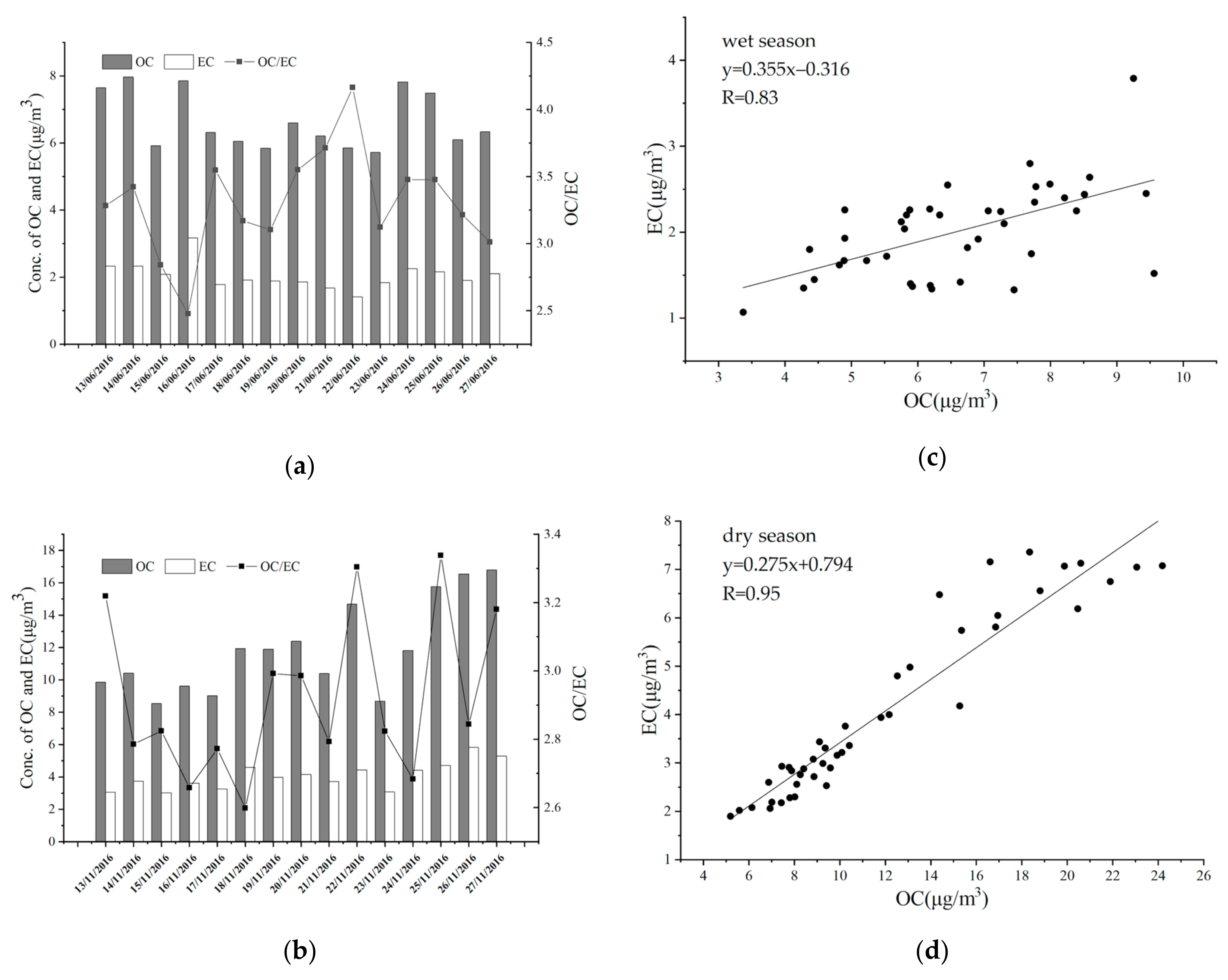
The mean concentrations of OC were 6.65 ± 0.85 μg/m3 and 11.88 ± 2.83 μg/m3 in the wet season and dry season, respectively. The mean EC concentrations were 2.04 ± 0.40 μg/m3 and 4.06 ± 0.83 μg/m3 in the wet season and dry season, respectively (Figure 5). Baoshan is located in the basin valley on the plateau, with wind speeds that are too low to be conducive to pollutant spreading during the two seasons. During the two sampling campaigns, the daily mean value of OC/EC was 2.48–4.16 in the wet season and 2.60–3.34 in the dry season, all of which exceeded 2.0, which indicated that Baoshan experienced secondary organic carbon (SOC) pollution in both seasons. Moreover, OC and EC in Baoshan had a better correlation in the dry season (R = 0.95) than that in the wet season (R = 0.83), which showed that the measured OC and EC were derived from similar sources during the dry season and from complex sources during the wet season. The possible reason for this is that the dry season is affected by the long-distance transmission of biomass combustion sources in Southeast Asia due to climatic conditions.

Figure 5.
Concentrations of OC and EC, the value of OC/EC, and the relevance of OC and EC in PM2.5 during the sampling period. (a) Concentrations of OC and EC in the wet season. (b) Concentrations of OC and EC in the dry season. (c) The value of OC/EC and the relevance of OC and EC in PM2.5 during the wet season sampling period. (d) The value of OC/EC and the relevance of OC and EC in PM2.5 during the dry season sampling period.
Since there is no simple and direct calculation method for SOC, this study estimates the content of SOC considering the lowest value of the OC/EC ratio in the two seasons [63,64,65]. The principle of this method is the use of the lowest value of OC/EC rather than that of the OC/EC of the primary pollutant in every season. SOC = TOC, EC × (OC/EC) min, and TOC and EC are the concentrations of OC and EC in PM2.5, respectively [66,67]. The average values of SOC in PM2.5 are 1.58 ± 0.66 μg/m3 and 1.34 ± 1.12 μg/m3 in the wet season and dry season, respectively. The values of SOC/OC in the two seasons are 23.76% and 11.28% in the wet and dry seasons, respectively. The radiation and temperature levels in the dry season were higher than those in the wet season, which represented more favorable photochemical conditions for the formation of SOC in the dry season. However, there was more rain in the wet season in Baoshan, which could limit the formation of SOC. The order of OC, SOC, and SOC/EC was the same pattern as the wet season >dry season, which meant that the impact of radiation and temperature was less than that of rainfall, and rainfall was the main influencing factor and had a greater impact on SOC [68,69].
3.3. Source Apportionment of PM2.5
3.3.1. Factor Profiles Results of PMF
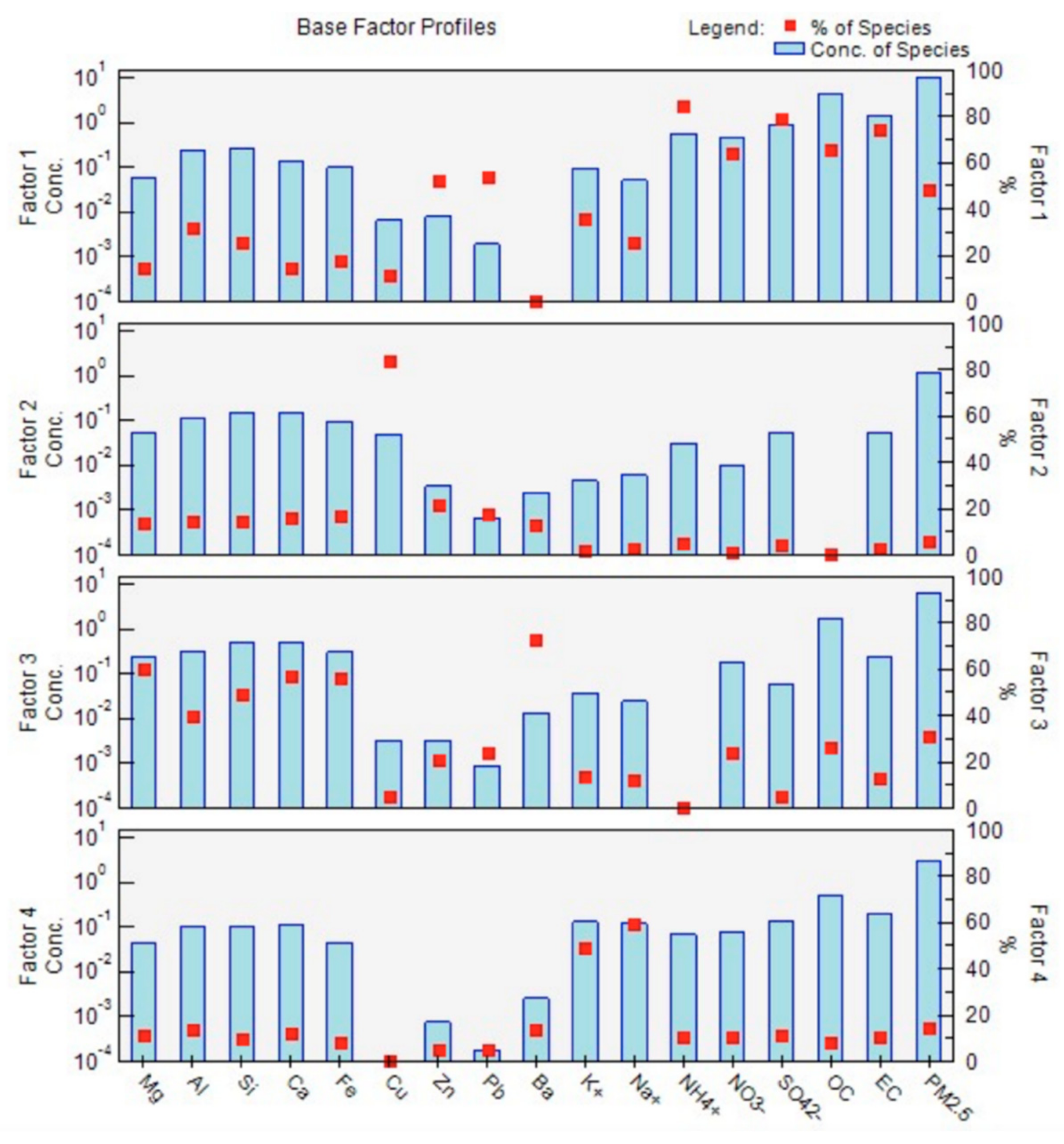
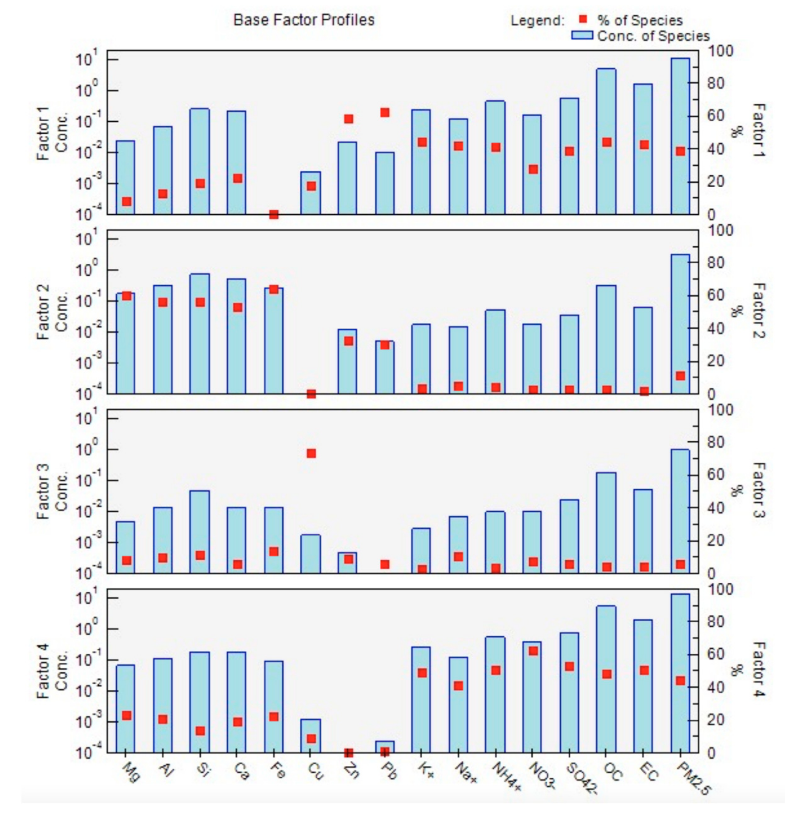
For the PMF model, 87 samples were put into it during the wet and dry seasons. According to the detection limit and signal-to-noise ratio, 16 species were finally retained in the wet season, and 15 species were retained in the dry season. To prevent double mass counting from affecting the results (Ca and Ca2+, K and K+, Na and Na+, Mg, and Mg2+) at the end of the analysis, only Na+, K+, Mg, and Ca were used. Species that were too far below the detection line are excluded. Materials of a similar origin, such as Ti, which is also a crustal element, were excluded. At the same time, the missing data was set as the median concentration, and its uncertainty was four times as high. The uncertainty of the additional modeling was set to 10% to achieve the most stable and physically interpretable solution.
The number of factors implemented in the PMF model ranged from 3–5, and it was found that when the number of factors was 4, the largest factor was the meaningful source of the dry and wet seasons. At the same time, the residuals of most species were between −3 and +3. When the number of factors increases, some species will be split, and the resulting factors are meaningless. The instability of rotation will also increase sharply.
To determine the uncertainty of a particular sample, the formula Sij = DL/3 + c × xij is used. Where Sij = uncertainty, DL = detection limit, C = constant (0.1 if xij > 3 × DL, 0.2 if xij < 3 × DL), and xij = variable [70].
After 20 basic runs, it was found that the lowest Qrobust was 499.3, and the Qrobust/Qtrue ratio was 0.97 during the wet season. During the dry season, the lowest Qrobust was 708.7, and the Qrobust/Qtrue ratio was 0.96. Please note that Qrobust/Qtrue < 2 means that it is generally acceptable [71]. After the application of the constraint, BS, DIS, and BS-DIS runs were conducted for evaluating the model’s solutions. In particular, 100 bootstrap runs were performed for each dataset (default minimum correlation R-value = 0.6), and the results were regarded reliable as >80% of the factors were mapped [72]. For more detailed results of the bootstrap program, please refer to Tables S2 and S3, Figures S1 and S2 in the supplementary file. In this study, Fpeak values between −1.0 and 0.5 (intervals of 0.1) gave convergent results with the minimum Q robust (1169.0), Q true (1191.2) was −0.1 in the wet season. The minimum Q robust (504.5.1), Q true (501.1) was −0.1 in the dry season. By altering the Fpeak value, it was not found to result in substantially better source profiles and contributions. Consequently, default base run results are reported in this paper. Figure 6 and Figure 7 show the PMF results in the wet season and dry season, respectively.
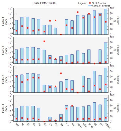
Figure 6.
Factor profiles: division of elements into individual factors, and their characterization from measurements of PM2.5 taken in the wet season in Baoshan.
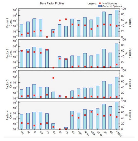
Figure 7.
Factor profiles: division of elements into individual factors, and their characterization from measurements of PM2.5 taken in the dry season in Baoshan.
The factor profile results generated by PMF analysis in the wet season are shown in Figure 6. Factor W1 is widely distributed in Zn, Pb, NH4+, NO3−, and SO42−, which is the generation of fossil fuel combustion and secondary inorganic particles [73,74,75,76], among the fossil fuel combustion source, including motor vehicle exhaust and coal combustion. Factor W2 has a large distribution on Cu, representing metal smelting, indicating that Baoshan is affected by copper smelting industries [77], which may come from local areas or Myanmar. The data show that Myanmar is rich in copper resources; Factor W3 is widely distributed on Mg, Al, Si, Ca and Ba, representing road dust source [78]; Factor W4 has a large distribution on Na+ and K+, representing sea salt and biomass combustion [79]. Sea salt may come from the Indian Ocean. No large amount of biomass combustion existed in June in the local area of Baoshan, so there may be a regional transport phenomenon of biomass burning in Baoshan.
The factor profile results generated by PMF analysis in the dry season are shown in Figure 7. Factor D1 has a large distribution of Zn, Pb, NH4+, OC, and EC, representing fossil fuel combustion; Factor D2 represents road dust, which is characterized by a high contribution of Mg, Al, Si, and Ca, which are crustal elements; Factor D3 has a large distribution on Cu, representing the source of copper smelting. Factor D4 is widely distributed in K+, NH4+, NO3−, SO42−, OC, and EC, indicating secondary sources and biomass combustion. It was also found that significant straw burning phenomenon exists in autumn in Baoshan, indicating that it is necessary to limit straw combustion activities to control air pollution [80].
It can be seen that the source analysis results of PM2.5 in Baoshan are approximately the same in the wet season and dry season. The main source of PM2.5 in the urban area of Baoshan came from fossil fuel combustion. It can be seen that motor vehicle exhaust and coal combustion have an important impact on the air quality of Baoshan. Controlling the number of motor vehicles and promoting green travel will help Baoshan to improve the air quality. In addition, it should be noted that the problem of straw burning in autumn in Baoshan needs to be solved, and government departments need to introduce relevant measures to curb the open-air burning of straw.
3.3.2. Relative Contributions from Sources of PM2.5 in Baoshan
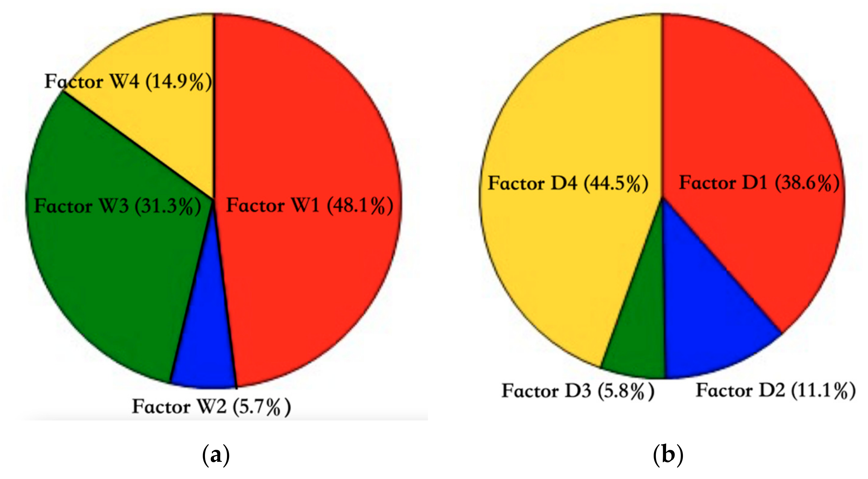
As shown in Figure 8a, the source contribution results of atmospheric PM2.5 show that the contribution rate of sources to PM2.5 in the wet season in Baoshan is as follows: fossil fuel combustion and secondary inorganic particles (48.1%) > road dust (31.3%) > biomass combustion and sea salt (14.9%) > metal smelting (5.7%). The contribution rate of fossil fuel combustion and secondary inorganic particles to PM2.5 is 48.1%, which is the largest source of PM2.5 in Baoshan; road dust is 31.3%, which is the second largest source of PM2.5 in Baoshan; biomass combustion and sea salt transportation and metal smelting, account for 14.9% and 5.7%, respectively.
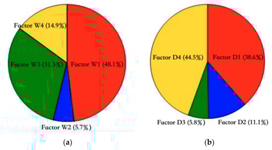
Figure 8.
(a) Source apportionment of PM2.5 in the wet season. Factor W1: Fossil fuel combustion and secondary inorganic particles; Factor W2: Metal smelting; Factor W3: Road dust; Factor W4: Biomass combustion and sea salt; (b) Source apportionment of PM2.5 in the dry season. Factor D1: Fossil fuel combustion; Factor D2: Road dust; Factor D3: Metal smelting; Factor D4: Biomass combustion and secondary inorganic particles.
As shown in Figure 8b, in the dry season, the contribution rate of various sources to PM2.5 is as follows: biomass combustion and secondary inorganic particles (44.5%) > fossil fuel combustion (38.6%) > road dust (11.1%) > metal smelting (5.8%). It can be seen that the straw burning in autumn in Baoshan had a great impact on the local air quality.
The PM2.5 sampling sites in Baoshan are less than 100 km away from Myanmar; therefore, it can be speculated that biomass combustion may come from cross-border transmission. There are a lot of copper resources in Myanmar [81], so the smelting of copper may also affect the air quality of Baoshan.
3.3.3. The Long-Range Transport
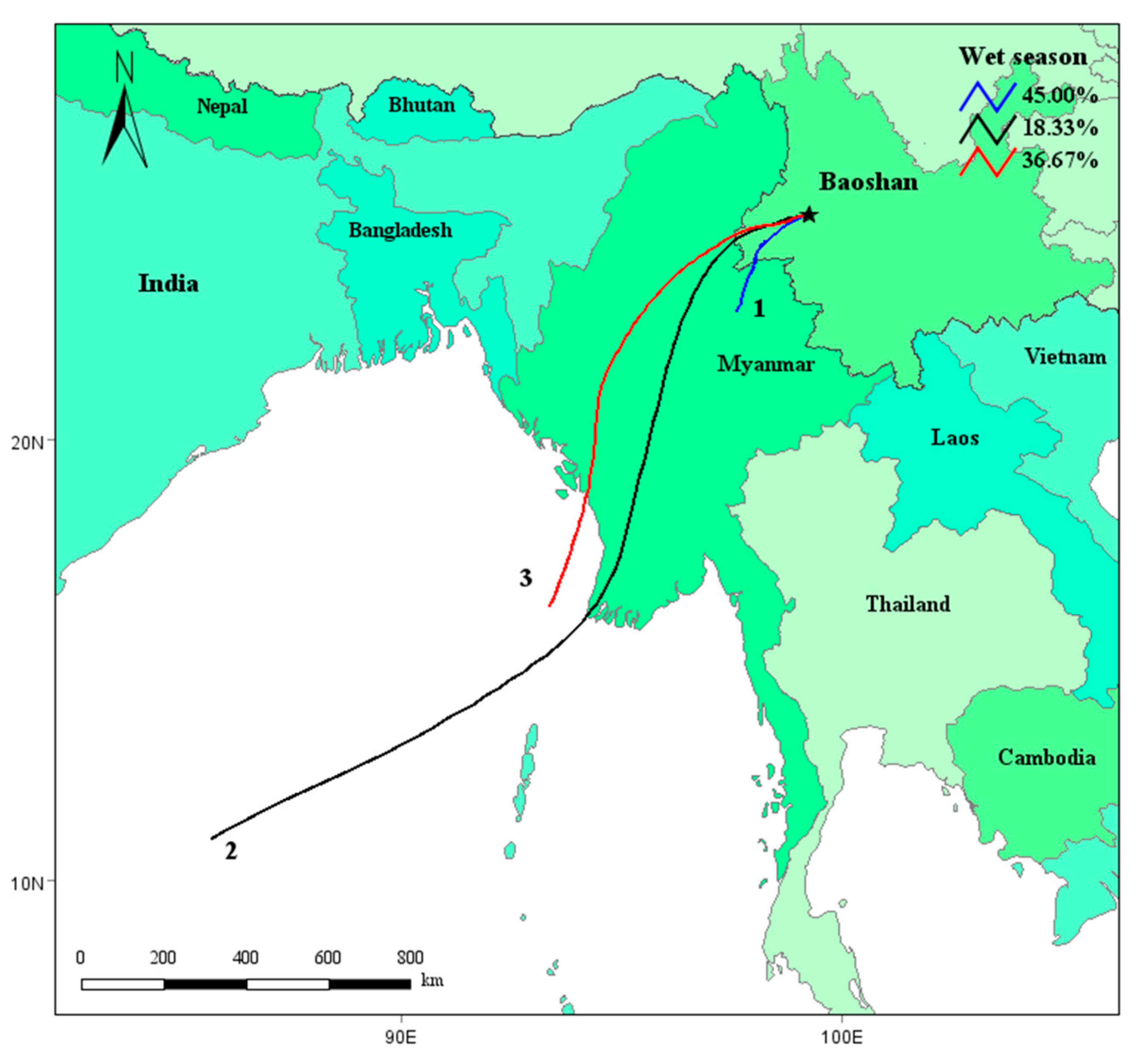
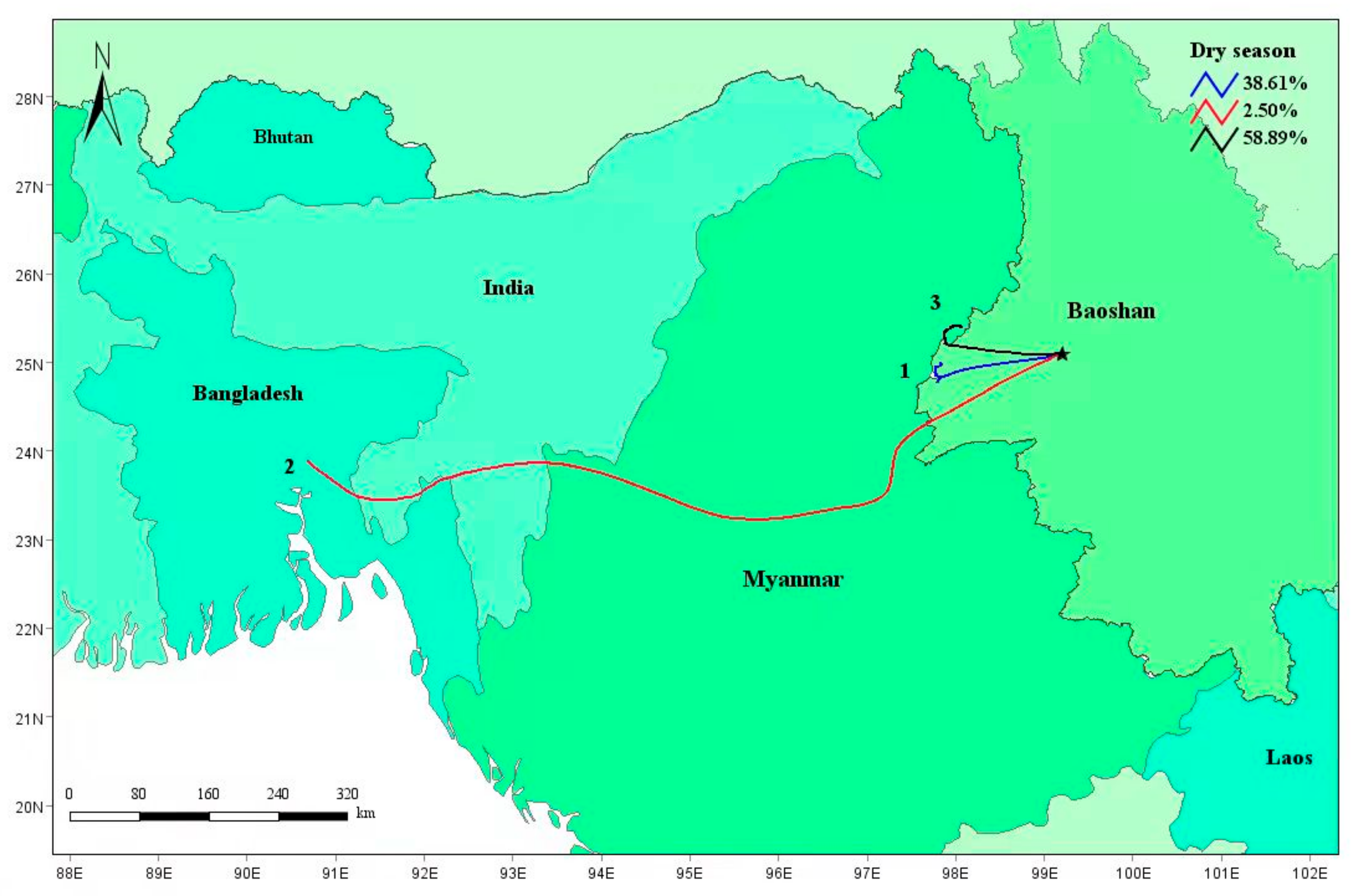
To better understand the transport of airborne particles from distant sources, the 72 h backward trajectories starting at a height of 1000 m at each sampling site were calculated using the Hybrid Single-Particle Lagrangian Integrated Trajectory 4.0 (HYSPLIT4) model with a 6 h period (meteorological data from the Global Data Assimilation System (GDAS)). The height in the article is the height relative to the ground. As there are many mountains in Southwest China and the altitude is high, if the altitude is set too low, the air mass trajectory model transported by the outside can not be well displayed. There were four tracks every day for 14 days, producing 64 tracks in total. In this paper, trajStat follow-up software was used to cluster the trajectory lines. The back trajectories were finally classified into three clusters using TrajStat in this study. Due to the fact that the spatial resolution of the backward trajectory model is not high, the whole Baoshan area could be used as a sampling site (25°10′ N, 99°17′ E) to calculate backward trajectories in the study. The time included the sampling days in June and November 2016. PM concentrations at the air parcel arrival are 7–8 μg/m3 in the wet season. The level was 12–13 μg/m3 in the dry season. It can be seen from Table 3 that the results in both the dry and wet seasons are due to the higher concentration of PM2.5 from the trajectory from the Myanmar area, while the corresponding PM2.5 concentration from the marine area was lower.
Table 3.
The level of the PM concentrations at the air parcel arrival (μg/m3).
As shown in Figure 9, in the wet season, the trajectories are divided into three groups. It can be seen that the three clusters were all in the southwest direction. One of the clusters accounted for 45.56% and came from the Myanmar region. Myanmar is rich in copper resources and frequent straw burning behaviors, which can explain the sources of metal smelting and biomass combustion in factor 4 of PMF in the wet season. Clusters No. 2 and No. 3 are all from the Indian Ocean, explaining the sea salt transport.
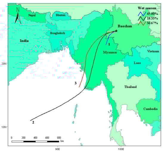
Figure 9.
The mean 72 h backward trajectories of each trajectory cluster during the wet season and the percentage of allocation to each cluster.
As shown in Figure 10, in the dry season, these trajectories mainly come from the west, the junction of Baoshan and Myanmar, and a small part comes from the southwest from Bangladesh and through Myanmar. This explains that the source of PM2.5 in the dry season in Baoshan City mainly comes from local biomass combustion; however, it can not be ruled out that any sources of biomass combustion come from the China and Myanmar border.

Figure 10.
The mean 72 h backward trajectories of each trajectory cluster during the dry season and the percentage of allocation to each cluster.
4. Conclusions
The mean concentrations of PM2.5 were 12.63 ± 4.75 μg/m3 and 34.45 ± 6.27 μg/m3 in the wet season and dry season. The air quality in Baoshan is better than that in most cities in China. WSIIs and OC were the main components of PM2.5, accounting for 19.87% and 34.43% of PM2.5, respectively. The ratio of NO3−/SO42− implied that the contribution of mobile sources was not significantly different from that of other cities. Fossil fuel combustion and secondary inorganic particles (48.1%), road dust (31.3%), biomass combustion and sea salt (14.9%), and metal smelting (5.7%) are the main sources of PM2.5 in the wet season. Biomass combustion and secondary inorganic particles (44.5%), fossil fuel combustion (38.6%), road dust (11.1%), and metal smelting (5.8%) are the main sources of PM2.5 in the dry season.
The cluster analysis results show that the long-distance migration of air pollutants has a profound impact on the local air quality in Baoshan, especially the air mass from Myanmar.
In this paper, the chemical composition and source characteristics of PM2.5 in a plateau border city were first studied, and the main sources of PM2.5 in Baoshan were resolved. The PMF source analysis model and the HYSPLIT 4 model were used to ensure that the PM2.5 source analysis results were accurate. The results can provide scientific data to support PM2.5 pollution control in local and similar cities. It can be seen that Baoshan needs to control the straw burning in autumn, as well as the emission of motor vehicle exhaust; therefore, the local government needs to take corresponding measures. At the same time, the impact of biomass combustion from Myanmar on air quality in Baoshan can also be found. In addition, Myanmar’s copper smelting may also affect the air quality in Baoshan. The problem of cross-border pollution also needs attention. Research results show that Baoshan’s air quality is affected to a certain extent by Myanmar. This has certain guiding significance for the Chinese government’s international cooperation projects in Southeast Asia.
Supplementary Materials
The following are available online at https://www.mdpi.com/article/10.3390/atmos13010007/s1, Figure S1: Output of the bootstrapping analysis in the wet season, Figure S2: Output of the bootstrapping analysis in the dry season, Table S1: Sampling time and weather conditions at three sampling sites in Baoshan, Table S2: Percent of bootstrap factors mapped back to the original PMF factors from the four-factor PMF solution in the wet season, Table S3: Percent of bootstrap factors mapped back to the original PMF factors from the four-factor PMF solution in the dry season.
Author Contributions
Conceptualization, J.S. and X.H.; investigation, Y.Z.; resources, X.H.; data curation, Z.W. and X.P.; writing—original draft preparation, C.Z.; writing—review and editing, J.S. and X.H.; supervision, P.N. All authors have read and agreed to the published version of the manuscript.
Funding
This research was funded by the National Key R&D Projects of China (grant number 2019YFC0214405) and the National Natural Science Foundation of China (grant number 21966016 and 21667014).
Institutional Review Board Statement
Not applicable.
Informed Consent Statement
Not applicable.
Data Availability Statement
The data used in this paper can be provided by Jianwu Shi (Shijianwu@kust.edu.cn).
Acknowledgments
This work was supported by the National Key Research and Development Projects of China and the National Natural Science Foundation of China.
Conflicts of Interest
The authors declare that there are no competing financial interest that could inappropriately influence the contents of this manuscript.
Nomenclature
| PM2.5 | Particulate matter with aerodynamic equivalent diameter less than or equal to 2.5 microns in ambient air |
| NOx | Refers to the sum of NO and NO2 |
| WSIIs | Water-soluble inorganic ions |
| OC | organic carbon |
| EC | inorganic carbon |
| IEs | inorganic elements |
| PMF | Positive definite matrix factorization |
| UV | Ultraviolet |
| BSC | Baoshan College |
| AA | Athlete apartmentns |
| EMS | Environmental Monitoring Station of Baoshan |
| ICP-AES | inductively coupled plasma-atomic emission spectrometry |
| DRI | Desert Institute |
| FID | lame ion detector |
| OPC | Organic pyrolysis carbon |
| IMPROVE | Interagency Monitoring of Protected Visual Environments |
| SIAs | Secondary inorganic aerosols (including NO3−, SO42− and NH4+) |
| CE/AE | Cation/Anion concentration ratio |
| NCEP | National Centers for Environmental Prediction |
| GDAS | Global Data Assimilation System |
| QC/QA | Quality control and Quality assurance |
References
- Zong, Z.; Wang, X.; Tian, C.; Chen, Y.; Qu, L.; Ji, L.; Zhi, G.; Li, J.; Zhang, G. Source apportionment of PM2.5 at a regional background site in North China using PMF linked with radiocarbon analysis: Insight into the contribution of biomass burning. Atmos. Chem. Phys. Discuss. 2016, 16, 11249–11265. [Google Scholar] [CrossRef] [Green Version]
- Li, Y.; Tao, J.; Zhang, L.; Jia, X.; Wu, Y. High Contributions of Secondary Inorganic Aerosols to PM2.5 under Polluted Levels at a Regional Station in Northern China. Int. J. Environ. Res. Public Health 2016, 13, 1202. [Google Scholar] [CrossRef] [PubMed] [Green Version]
- Lu, D.; Xu, J.; Yang, D.; Zhao, J. Spatio-temporal variation and influence factors of PM2.5 concentrations in China from 1998 to 2014. Atmos. Pollut. Res. 2017, 8, 1151–1159. [Google Scholar] [CrossRef]
- Samresh, K.; Ramya, S.R. Inorganic ions in ambient fine particles over a National Park in central India: Seasonality, dependencies between SO42−, NO3− and NH4+, and neutralization of aerosol acidity. Atmos. Environ. 2016, 143, 152–163. [Google Scholar]
- Georgoulias, A.K.; Marinou, E.; Tsekeri, A.; Proestakis, E.; Akritidis, D.; Alexandri, G.; Zanis, P.; Balis, D.; Marenco, F.; Tesche, M.; et al. A First Case Study of CCN Concentrations from Spaceborne Lidar Observations. Remote Sens. 2020, 12, 1557. [Google Scholar] [CrossRef]
- Turap, Y.; Talifu, D.; Wang, X.; Abulizi, A.; Maihemuti, M.; Tursun, Y.; Rekefu, S. Temporal distribution and source appor-tionment of PM2.5 chemical composition in Xinjiang, NW-China. Atmos. Res. 2019, 218, 257–268. [Google Scholar] [CrossRef]
- Qiao, B.; Chen, Y.; Tian, M.; Wang, H.; Yang, F.; Shi, G.; Zhang, L.; Peng, C.; Luo, Q.; Ding, S. Characterization of water soluble inorganic ions and their evolution processes during PM2.5 pollution episodes in a small city in southwest China. Sci. Total Environ. 2019, 650, 2605–2613. [Google Scholar] [CrossRef]
- Tian, S.; Liu, Y.; Wang, J.; Wang, J.; Hou, L.; Lv, B.; Wang, X.; Zhao, X.; Yang, W.; Geng, C.; et al. Chemical Compositions and Source Analysis of PM2.5 during Autumn and Winter in a Heavily Polluted City in China. Atmosphere 2020, 11, 336. [Google Scholar] [CrossRef] [Green Version]
- Guo, W.; Long, C.; Zhang, Z.; Zheng, N.; Xiao, H.; Xiao, H. Seasonal Control of Water-Soluble Inorganic Ions in PM2.5 from Nanning, a Subtropical Monsoon Climate City in Southwestern China. Atmosphere 2019, 11, 5. [Google Scholar] [CrossRef] [Green Version]
- Zhang, J.; Tong, L.; Huang, Z.; Zhang, H.; He, M.; Dai, X.; Zheng, J.; Xiao, H. Seasonal variation and size distributions of water-soluble inorganic ions and carbonaceous aerosols at a coastal site in Ningbo, China. Sci. Total Environ. 2018, 639, 793–803. [Google Scholar] [CrossRef] [PubMed]
- Dong, Z.; Su, F.; Zhang, Z.; Wang, S. Observation of chemical components of PM2.5 and secondary inorganic aerosol formation during haze and sandy haze days in Zhengzhou, China. J. Environ. Sci. 2020, 88, 316–325. [Google Scholar] [CrossRef] [PubMed]
- Golly, B.; Waked, A.; Weber, S.; Samake, A.; Jacob, V.; Conil, S.; Rangognio, J.; Chrétien, E.; Vagnot, M.-P.; Robic, P.-Y.; et al. Organic markers and OC source apportionment for seasonal variations of PM2.5 at 5 rural sites in France. Atmos. Environ. 2019, 198, 142–157. [Google Scholar] [CrossRef]
- Jin, Q.; Fang, X.; Wen, B.; Shan, A. Spatio-temporal variations of PM2.5 emission in China from 2005 to 2014. Chemosphere 2017, 183, 429–436. [Google Scholar] [CrossRef] [PubMed]
- Siudek, P.; Frankowski, M. Atmospheric deposition of trace elements at urban and forest sites in central Poland—Insight into seasonal variability and sources. Atmos. Res. 2017, 198, 123–131. [Google Scholar] [CrossRef]
- Guan, Q.; Liu, Z.; Yang, L.; Luo, H.; Yang, Y.; Zhao, R.; Wang, F. Variation in PM2.5 source over megacities on the ancient Silk Road, northwestern China. J. Clean. Prod. 2019, 208, 897–903. [Google Scholar] [CrossRef]
- Rohra, H.; Pipal, A.S.; Tiwari, R.; Vats, P.; Masih, J.; Khare, P.; Taneja, A. Particle size dynamics and risk implication of atmospheric aerosols in South-Asian subcontinent. Chemosphere 2020, 249, 126140. [Google Scholar] [CrossRef] [PubMed]
- Dai, Q.; Bi, X.; Liu, B.; Li, L.; Ding, J.; Song, W.; Bi, S.; Schulze, B.C.; Song, C.; Wu, J.; et al. Chemical nature of PM2.5 and PM10 in Xi’an, China: Insights into primary emissions and secondary particle formation. Environ. Pollut. 2018, 240, 155–166. [Google Scholar] [CrossRef] [PubMed]
- Wang, S.; Yu, R.; Shen, H.; Wang, S.; Hu, Q.; Cui, J.; Yan, Y.; Huang, H.; Hu, G. Chemical characteristics, sources, and formation mechanisms of PM2.5 before and during the Spring Festival in a coastal city in Southeast China. Environ. Pollut. 2019, 251, 442–452. [Google Scholar] [CrossRef] [PubMed]
- Xie, Y.; Liu, Z.; Wen, T.; Huang, X.; Liu, J.; Tang, G.; Yang, Y.; Li, X.; Shen, R.; Hu, B.; et al. Characteristics of chemical composition and seasonal variations of PM2.5 in Shijiazhuang, China: Impact of primary emissions and secondary formation. Sci. Total Environ. 2019, 677, 215–229. [Google Scholar] [CrossRef]
- Souto-Oliveira, C.; Babinski, M.; Araújo, D.; Weiss, D.; Ruiz, I. Multi-isotope approach of Pb, Cu and Zn in urban aerosols and anthropogenic sources improves tracing of the atmospheric pollutant sources in megacities. Atmos. Environ. 2019, 198, 427–437. [Google Scholar] [CrossRef] [Green Version]
- Li, R.; Hardy, R.; Zhang, W.; Reinbold, G.L.; Strachan, S.M. Chemical Characterization and Source Apportionment of PM2.5 in a Nonattainment Rocky Mountain Valley. J. Environ. Qual. 2018, 47, 238–245. [Google Scholar] [CrossRef] [PubMed] [Green Version]
- Wang, H.; Qiao, L.; Lou, S.; Zhou, M.; Ding, A.; Huang, H.; Chen, J.; Wang, Q.; Tao, S.; Chen, C.; et al. Chemical composition of PM2.5 and meteorological impact among three years in urban Shanghai, China. J. Clean. Prod. 2016, 112, 1302–1311. [Google Scholar] [CrossRef]
- Cao, L.; Zhu, Q.; Huang, X.; Deng, J.; Chen, J.; Hong, Y.; Xu, L.; He, L. Chemical characterization and source apportionment of atmospheric submicron particles on the western coast of Taiwan Strait, China. J. Environ. Sci. 2017, 52, 293–304. [Google Scholar] [CrossRef] [PubMed]
- Zhu, W.; Xu, X.; Zheng, J.; Yan, P.; Wang, Y.; Cai, W. The characteristics of abnormal wintertime pollution events in the Jing-Jin-Ji region and its relationships with meteorological factors. Sci. Total Environ. 2018, 626, 887–898. [Google Scholar] [CrossRef] [PubMed]
- Li, J.; Bi, L.; Han, X.; Shi, J.; Yang, J.; Shi, Z.; Ning, P. Characteristics and source apportionment of the water soluble inorganic ions in PM2.5 of Kunming. J. Yunnan Univ. 2017, 39, 63–70. (In Chinese) [Google Scholar]
- Bi, L.; Hao, J.; Ning, P.; Shi, J.; Shi, Z.; Xu, X. Characteristics and sources apportionment of PM2.5-bound PAHs in Kunming. China Environ. Sci. 2015, 35, 659–667. (In Chinese) [Google Scholar]
- Wang, C.-H.; Yan, K.; Han, X.-Y.; Shi, Z.; Bi, L.-M.; Xiang, F.; Ning, P.; Shi, J.-W. Physico-chemical Characteristic Analysis of PM2.5 in the Highway Tunnel in the Plateau City of Kunming. Environ. Sci. 2017, 38, 4968–4975. (In Chinese) [Google Scholar]
- Han, L.; Huang, J.; Han, X.; Yang, J.; Shi, J.; Zhang, C.; Ning, P. Characteristics and Sources of Heavy Metals in Atmospheric PM2.5 Research during the Dry Season in Kunming. J. Kunming Univ. Sci. Technol. Nat. Sci. 2019, 44, 99–110. (In Chinese) [Google Scholar]
- Sun, Z.-R.; Ji, Z.-Y.; Han, X.-Y.; Shi, J.-W.; Zhang, J.; Zhang, C.-N.; Ning, P. Spatial and temporal characteristics of atmospheric VOCs and other pollutants concentrations in urban air of Yuxi City. J. Yunnan Univ. 2018, 40, 705–715. (In Chinese) [Google Scholar]
- Shi, Z.; Bi, L.; Shi, J.; Xiang, F.; Qian, L.; Ning, P. Characterization and Source Identification of PM2.5 in Ambient Air of Kunming in Windy Spring. Environ. Sci. Technol. 2014, 37, 143–147. (In Chinese) [Google Scholar]
- Paatero, P.; Hopke, P.K. Rotational tools for factor analytic models. J. Chemom. 2009, 23, 91–100. [Google Scholar] [CrossRef]
- Paatero, P.; Eberly, S.; Brown, S.G.; Norris, G.A. Methods for estimating uncertainty in factor analytic solutions. Atmos. Meas. Tech. 2014, 7, 781–797. [Google Scholar] [CrossRef] [Green Version]
- Paatero, P.; Tapper, U. Positive matrix factorization: A non-negative factor model with optimal utilization of error estimates of data values. Environmetrics 1994, 5, 111–126. [Google Scholar] [CrossRef]
- Paatero, P. Least squares formulation of robust non-negative factor analysis. Chemom. Intell. Lab. Syst. 1997, 37, 23–35. [Google Scholar] [CrossRef]
- Nicolás, J.; Chiari, M.; Crespo, J.; Orellana, I.G.; Lucarelli, F.; Nava, S.; Pastor, C.; Yubero, E. Quantification of Saharan and local dust impact in an arid Mediterranean area by the positive matrix factorization (PMF) technique. Atmos. Environ. 2008, 42, 8872–8882. [Google Scholar] [CrossRef]
- Liao, H.-T.; Chou, C.C.-K.; Chow, J.C.; Watson, J.; Hopke, P.; Wu, C.-F. Source and risk apportionment of selected VOCs and PM2.5 species using partially constrained receptor models with multiple time resolution data. Environ. Pollut. 2015, 205, 121–130. [Google Scholar] [CrossRef] [PubMed]
- Escrig, A.; Monfort, E.; Celades, I.; Querol, X.; Amato, F.; Minguillón, M.C.; Hopke, P.K. Application of Optimally Scaled Target Factor Analysis for Assessing Source Contribution of Ambient PM10. J. Air Waste Manag. Assoc. 2009, 59, 1296–1307. [Google Scholar] [CrossRef] [PubMed]
- Zhao, P.S.; Dong, F.; He, D.; Zhao, X.J.; Zhang, X.L.; Zhang, W.Z.; Yao, Q.; Liu, H.Y. Characteristics of concentrations and chemical compositions for PM2.5 in the region of Beijing, Tianjin, and Hebei, China. Atmos. Chem. Phys. Discuss. 2013, 13, 4631–4644. [Google Scholar] [CrossRef] [Green Version]
- Liu, N.; Feng, X.; Matthew, L.; Chen, Z.; Qiu, G. Pollution Characteristics of PM2.5 in Guiyang and Its Influence on Meteorological Parameters. Earth Environ. 2014, 42, 311–315. (In Chinese) [Google Scholar]
- Shi, J.; Feng, Y.; Ren, L.; Lu, X.; Zhong, Y.; Han, X.; Ning, P. Mass Concentration, Chemical Composition, and Source Characteristics of PM2.5 in a Plateau Slope City in Southwest China. Atmosphere 2021, 12, 611. [Google Scholar] [CrossRef]
- Ac, A.; Rps, B. Decline in PM2.5 concentrations over major cities around the world associated with COVID-19. Environ. Res. 2020, 187, 109634. [Google Scholar]
- Cheng, C.; Shi, M.; Liu, W.; Mao, Y.; Hu, J.; Tian, Q.; Chen, Z.; Hu, T.; Xing, X.; Qi, S. Characteristics and source apportionment of water-soluble inorganic ions in PM2.5 during a wintertime haze event in Huanggang, central China. Atmos. Pollut. Res. 2021, 12, 111–123. [Google Scholar] [CrossRef]
- Sharma, S.; Mandal, T. Chemical composition of fine mode particulate matter (PM2.5) in an urban area of Delhi, India and its source apportionment. Urban Clim. 2017, 21, 106–122. [Google Scholar] [CrossRef]
- Li, W.; Wang, X.; Zhang, Y. Influence of PRD Industrial Emission Variation on Concentrations of SO2, NOx and their Secondary Pollutants. Res. Environ. Sci. 2009, 22, 207–214. (In Chinese) [Google Scholar]
- Wang, H.; An, J.; Cheng, M.; Shen, L.; Zhu, B.; Li, Y.; Wang, Y.; Duan, Q.; Sullivan, A.; Xia, L. One year online measurements of water-soluble ions at the industrially polluted town of Nanjing, China: Sources, seasonal and diurnal variations. Chemosphere 2016, 148, 526–536. [Google Scholar] [CrossRef]
- Wang, Y.; Zhuang, G.; Zhang, X.; Huang, K.; Xu, C.; Tang, A.; Chen, J.; An, Z. The ion chemistry, seasonal cycle, and sources of PM2.5 and TSP aerosol in Shanghai. Atmos. Environ. 2006, 40, 2935–2952. [Google Scholar] [CrossRef]
- He, Q.; Yan, Y.; Guo, L.; Zhang, Y.; Zhang, G.; Wang, X. Characterization and source analysis of water-soluble inorganic ionic species in PM2.5 in Taiyuan city, China. Atmos. Res. 2017, 184, 48–55. [Google Scholar] [CrossRef]
- Rengarajan, R.; Sudheer, A.; Sarin, M. Wintertime PM2.5 and PM10 carbonaceous and inorganic constituents from urban site in western India. Atmos. Res. 2011, 102, 420–431. [Google Scholar] [CrossRef]
- Mostafa, A.N.; Zakey, A.S.; Alfaro, S.C.; Wheida, A.A.; Monem, S.A.; Wahab, M.M.A. Validation of RegCM-CHEM4 model by comparison with surface measurements in the Greater Cairo (Egypt) megacity. Environ. Sci. Pollut. Res. Int. 2019, 26, 23524–23541. [Google Scholar] [CrossRef] [PubMed]
- Qiu, T.; Zhou, J.; Xiao, J.; Guo, H.; Yu, W. Characteristics and sources apportionment of water-soluble ions in PM2.5 in autumn and winter of Wuhan. Environ. Pollut. Control 2015, 37, 17–20. (In Chinese) [Google Scholar]
- Sun, Y.; Zhuang, G.; Wang, Y.; Han, L.; Guo, J.; Dan, M.; Zhang, W.; Wang, Z.; Hao, Z. The air-borne particulate pollution in Beijing—Concentration, composition, distribution and sources. Atmos. Environ. 2004, 38, 5991–6004. [Google Scholar] [CrossRef]
- Zhang, T.; Cao, J.; Tie, X.; Shen, Z.; Liu, S.; Ding, H.; Han, Y.; Wang, G.; Ho, K.F.; Qiang, J.; et al. Water-soluble ions in atmospheric aerosols measured in Xi’an, China: Seasonal variations and sources. Atmos. Res. 2011, 102, 110–119. [Google Scholar] [CrossRef]
- Wang, P.; Cao, J.-J.; Shen, Z.-X.; Han, Y.-M.; Lee, S.-C.; Huang, Y.; Zhu, C.-S.; Wang, Q.-Y.; Xu, H.-M.; Huang, R.-J. Spatial and seasonal variations of PM2.5 mass and species during 2010 in Xi’an, China. Sci. Total Environ. 2015, 508, 477–487. [Google Scholar] [CrossRef]
- Zhou, M.; Qiao, L.; Zhu, S.; Li, L.; Lou, S.; Wang, H.; Wang, Q.; Tao, S.; Huang, C.; Chen, C. Chemical characteristics of fine particles and their impact on visibility impairment in Shanghai based on a 1-year period observation. J. Environ. Sci. 2016, 48, 151–160. [Google Scholar] [CrossRef]
- Hu, M.; He, L.-Y.; Zhang, Y.-H.; Wang, M.; Kim, Y.P.; Moon, K. Seasonal variation of ionic species in fine particles at Qingdao, China. Atmos. Environ. 2002, 36, 5853–5859. [Google Scholar] [CrossRef]
- Fang, G.-C.; Chang, C.-N.; Wu, Y.-S.; Fu, P.P.-C.; Yang, C.-J.; Chen, C.-D.; Chang, S.-C. Ambient suspended particulate matters and related chemical species study in central Taiwan, Taichung during 1998–2001. Atmos. Environ. 2002, 36, 1921–1928. [Google Scholar] [CrossRef]
- Bhuyan, P.; Deka, P.; Prakash, A.; Balachandran, S.; Hoque, R.R. Chemical characterization and source apportionment of aerosol over mid Brahmaputra Valley, India. Environ. Pollut. 2018, 234, 997–1010. [Google Scholar] [CrossRef]
- Meng, C.; Wang, L.; Zhang, F.; Wei, Z.; Ma, S.; Ma, X.; Yang, J. Characteristics of concentrations and water-soluble inorganic ions in PM2.5 in Handan City, Hebei province, China. Atmos. Res. 2016, 171, 133–146. [Google Scholar] [CrossRef]
- Yang, Y.; Zhou, R.; Yu, Y.; Yan, Y.; Liu, Y.; Di, Y.; Wu, D.; Zhang, W. Size-resolved aerosol water-soluble ions at a regional background station of Beijing, Tianjin, and Hebei, North China. J. Environ. Sci. 2017, 55, 146–156. [Google Scholar] [CrossRef]
- Huang, L.; Wang, G. Chemical characteristics and source apportionment of atmospheric particles during heating period in Harbin, China. J. Environ. Sci. 2014, 26, 2475–2483. [Google Scholar] [CrossRef] [PubMed]
- Lv, S.; Shao, L.; Wu, M. Characteristics of Chemical Elements in Beijing PM10 and Their Source Apportionment. J. China Univ. Min. Technol. 2006, 35, 685–688. (In Chinese) [Google Scholar]
- Pakkanen, T.A.; Loukkola, K.; Korhonen, C.H.; Aurela, M.; Mäkelä, T.; Hillamo, R.E.; Aarnio, P.; Koskentalo, T.; Kousa, A.; Maenhaut, W. Sources and chemical composition of atmospheric fine and coarse particles in the Helsinki area. Atmos. Environ. 2001, 35, 5381–5391. [Google Scholar] [CrossRef]
- Chu, S.-H. Stable estimate of primary OC/EC ratios in the EC tracer method. Atmos. Environ. 2005, 39, 1383–1392. [Google Scholar] [CrossRef]
- Wang, T.; Nie, W.; Gao, J.; Xue, L.K.; Gao, X.M.; Wang, X.F.; Qiu, J.; Poon, C.N.; Meinardi, S.; Blake, D.; et al. Air quality during the 2008 Beijing Olympics: Secondary pollutants and regional impact. Atmos. Chem. Phys. Discuss. 2010, 10, 7603–7615. [Google Scholar] [CrossRef] [Green Version]
- Rotivit, L.; Jacobsen, D. Temperature increase and respiratory performance of macroinvertebrates with different tolerances to organic pollution. Limnologica 2013, 43, 510–515. [Google Scholar] [CrossRef]
- Cheng, S.-Y.; Liu, C.; Han, L.-H.; Li, Y.; Wang, Z.; Tian, C. Characteristics and Source Apportionment of Organic Carbon and Elemental Carbon in PM2.5 During the Heating Season in Beijing. J. Beijing Univ. Technol. 2014, 40, 586–591. (In Chinese) [Google Scholar]
- Tan, J.; Duan, J.; He, K.; Ma, Y.; Duan, F.; Chen, Y.; Fu, J. Chemical characteristics of PM2.5 during a typical haze episode in Guangzhou. J. Environ. Sci. 2009, 21, 774–781. [Google Scholar] [CrossRef]
- Zhang, C.; Lu, X.; Zhai, J.; Chen, H.; Yang, X.; Zhang, Q.; Zhao, Q.; Fu, Q.; Sha, F.; Jin, J. Insights into the formation of secondary organic carbon in the summertime in urban Shanghai. J. Environ. Sci. 2018, 72, 118–132. [Google Scholar] [CrossRef]
- Zhang, Q.; Sarkar, S.; Wang, X.; Zhang, J.; Mao, J.; Yang, L.; Shi, Y.; Jia, S. Evaluation of factors influencing secondary organic carbon (SOC) estimation by CO and EC tracer methods. Sci. Total Environ. 2019, 686, 915–930. [Google Scholar] [CrossRef]
- Chueinta, W.; Hopke, P.; Paatero, P. Investigation of sources of atmospheric aerosol at urban and suburban residential areas in Thailand by positive matrix factorization. Atmos. Environ. 2000, 34, 3319–3329. [Google Scholar] [CrossRef]
- Baumann, K.; Jayanty, R.; Flanagan, J.B. Fine Particulate Matter Source Apportionment for the Chemical Speciation Trends Network Site at Birmingham, Alabama, Using Positive Matrix Factorization. J. Air Waste Manag. Assoc. 2008, 58, 27–44. [Google Scholar] [CrossRef] [Green Version]
- Saraga, D.E.; Tolis, E.I.; Maggos, T.; Vasilakos, C.; Bartzis, J.G. PM2.5 source apportionment for the port city of Thessaloniki, Greece. Sci. Total Environ. 2019, 650, 2337–2354. [Google Scholar] [CrossRef] [PubMed]
- Marcazzan, G.M.; Vaccaro, S.; Valli, G.; Vecchi, R. Characterisation of PM10 and PM2.5 particulate matter in the ambient air of Milan (Italy). Atmos. Environ. 2001, 35, 4639–4650. [Google Scholar] [CrossRef]
- Pacyna, J.M.; Pacyna, E.G. An assessment of global and regional emissions of trace metals to the atmosphere from anthropogenic sources worldwide. Environ. Rev. 2001, 9, 269–298. [Google Scholar] [CrossRef]
- Manousakas, M.; Diapouli, E.; Papaefthymiou, H.; Migliori, A.; Karydas, A.; Padilla-Alvarez, R.; Bogovac, M.; Kaiser, R.; Jaksic, M.; Bogdanovic-Radovic, I.; et al. Source apportionment by PMF on elemental concentrations obtained by PIXE analysis of PM10 samples collected at the vicinity of lignite power plants and mines in Megalopolis, Greece. Nucl. Instrum. Methods Phys. Res. Sect. B Beam Interact. Mater. Atoms 2015, 349, 114–124. [Google Scholar] [CrossRef]
- Kim, E.; Larson, T.V.; Hopke, P.K.; Slaughter, C.; Sheppard, L.E.; Claiborn, C. Source identification of PM2.5 in an arid Northwest U.S. City by positive matrix factorization. Atmos. Res. 2003, 66, 291–305. [Google Scholar] [CrossRef]
- Shridhar, V.; Khillare, P.S.; Agarwal, T.; Ray, S. Metallic species in ambient particulate matter at rural and urban location of Delhi. J. Hazard. Mater. 2010, 175, 600–607. [Google Scholar] [CrossRef] [PubMed]
- Ivošević, T.; Stelcer, E.; Orlić, I.; Radović, I.B.; Cohen, D. Characterization and source apportionment of fine particulate sources at Rijeka, Croatia from 2013 to 2015. Nucl. Instrum. Methods Phys. Res. Sect. B Beam Interact. Mater. Atoms 2016, 371, 376–380. [Google Scholar] [CrossRef]
- Pey, J.; Pérez, N.; Cortés, J.; Alastuey, A.; Querol, X. Chemical fingerprint and impact of shipping emissions over a western Mediterranean metropolis: Primary and aged contributions. Sci. Total Environ. 2013, 463–464, 497–507. [Google Scholar] [CrossRef] [PubMed]
- Tipayarom, D.; Thi, N.; Oanh, K. Effects from Open Rice Straw Burning Emission on Air Quality in the Bangkok Metropolitan Region. Sci. Asia 2007, 33, 339–345. [Google Scholar] [CrossRef]
- Aung, T.S.; Shengji, L.; Condon, S. Evaluation of the environmental impact assessment (EIA) of Chinese EIA in Myanmar: Myitsone Dam, the Lappadaung Copper Mine and the Sino-Myanmar oil and gas pipelines. Impact Assess. Proj. Apprais. 2019, 37, 71–85. [Google Scholar] [CrossRef]


Publisher’s Note: MDPI stays neutral with regard to jurisdictional claims in published maps and institutional affiliations. |
© 2021 by the authors. Licensee MDPI, Basel, Switzerland. This article is an open access article distributed under the terms and conditions of the Creative Commons Attribution (CC BY) license (https://creativecommons.org/licenses/by/4.0/).