1. Introduction
Lake Baikal is a unique natural object with special requirements for its ecological state, which is becoming increasingly more challenging to maintain due to climatic changes observed in the basin of the lake catchment over the past decades [
1,
2,
3]. This is largely associated with seasonal and interannual fluctuations in its water level, which depend on the inflow into the lake, water flow through the Irkutsk HPP (located near the source of the Angara—the only river flowing from the lake), and evaporation from the water surface. Effective inflow is determined by a surface inflow of rivers flowing into the lake (there are more than 300 of them) less evaporation from its surface. The average annual hydrograph of the lake is quarterly determined as a percentage: 4, 38, 54, 4%. The inflows in the first and fourth quarters play no significant role. The evaporation from the lake surface is appreciable only in hot, low-water summers and, especially, before the ice cover establishment, when effective inflow becomes negative. Whereas the effective inflow in the second quarter is related to snow melting in mountainous areas of rivers and can be partially predicted by snow reserves, in the third quarter, it is determined exclusively by rainfall in the catchment basin of the lake [
4,
5].
The most crucial ecological and water management requirements for the regulation of the lake level are the restrictions introduced for the minimum level in April of 456 m (the Pacific Height System) and the maximum level in September–October of 457 m, which are difficult or impossible to fulfill in the case of small or high effective inflow.
Since the effective inflow to the lake has a probabilistic nature with significant seasonal and interannual variability (it can vary from extreme dry periods to catastrophic floods), effective management of the lake level and water flow through the Irkutsk HPP is a challenging task [
4,
5]. This situation is due to the currently unavailable reliable long-term prognostic estimates of water inflow into the lake for a period of up to one year (long-term forecast in meteorology is defined in the range of one month to two years).
At present, there is no generally accepted methodology for long-term forecasting of the effective inflow to manage the level of Lake Baikal, which is due to the unreliability of forecast estimates resulting from the specific features of the lake catchment basin. In this research, the basin is represented by two large heterogeneous parts: the Selenga river basin and the remaining part. The Selenga River is responsible for about 50% of the total runoff into Lake Baikal and determines long dry periods and extremely high water content in the lake.
In the absence of reliable forecasts, we propose a technology to make long-term forecasting estimations of effective inflow into the lake and their periodic refinement. The technology relies on neural network models of preliminary inflow estimates for a period of up to a year and continuous monitoring of the state of the atmosphere using a specialized technology for processing ensemble forecasts of the global CFSv2 model [
6,
7,
8,
9]. Refinement also involves neural network models, which is related to emerging new available predictors as the studied periods come nearer. This approach allows adjusting prognostic estimates in advance in the case of global atmospheric changes, which were not considered in the ensemble forecasts.
Continuous monitoring of current and prognostic distributions of surface temperatures, humidity, precipitation, and other parameters of the atmospheric state in the basin of Lake Baikal can provide us in advance with the most probable estimates of the final inflow availability already by the middle of the year to plan the next water management season, and, if necessary (for example, with a significant change in atmospheric parameters), to promptly adjust them.
The presented work addresses the method of monitoring the state of the atmosphere and long-term forecast estimations of inflow based on the GeoGIPSAR [
10] system implemented at the Melentiev Energy Systems Institute of Siberian Branch of the Russian Academy of Sciences (MESI SB RAS).
2. Materials and Methods
2.1. Initial Data. Organization of Monitoring of the Atmospheric State Data
Currently, there is a whole host of electronic resources with open access to archival data on actual indicators of the state of the atmosphere with a variety of spatial and temporal resolutions (for example, [
11,
12,
13]). Long-term prognostic estimates require indicators for a decade, a month, or a season, for which the temporal detailing for one day or even a month is sufficient. Many Internet services have also been developed to monitor current and prognostic indicators of the atmosphere for several days based on data generated by global climate models, for example, the services discussed in [
14,
15,
16].
The proposed approach to monitoring actual indicators of atmospheric parameters in the basin of Lake Baikal employs retrospective analysis for all layers of troposphere and stratosphere in a diurnal resolution for the period of 1948–2021, relying on the data from NOAA/NCEP [
13] with a coordinate grid of 2.5 × 2.5°; GPCC [
17,
18,
19,
20,
21,
22] based on precipitation with a monthly resolution for the period of 1900–2020 and a coordinate grid of 1 × 1°; archival [
23] and operational [
24] actual indicators for the considered basin in a monthly and daily resolution for any observation period starting from the end of the 19th century. Data from observation points in the basin allow verifying and refining the retrospective analysis data. For the effectiveness of further analysis, the initial data from the HDF5 format are converted into a specialized GI3-format, which makes it possible to store not only spatial data over the entire observation period in one file, but also include indicators of average, minimum, and maximum values for each date in this file.
Based on the analysis of global climatic indicators [
25,
26], we have identified the relationships between the variability of atmospheric circulation in the basin and the total inflow into it. These relationships are used to form potential predictors and adjust multivariate neural networks according to the prognostic interval estimates of inflow.
A dedicated technology was developed to process forecast ensembles produced by the global climate system CFSv2 [
6,
7,
8,
9] to obtain predictive estimates of the temperature, precipitation intensity, and surface pressure distributions. This technology taken into account of the dynamics of changes in atmospheric circulation, ocean currents, and ice conditions in the Arctic and Antarctic. Technology was also developed to convert the original information (in GRIB format) into specialized files of the CFS format with average daily prognostic indicators and direct access to their elements and their storage in the data warehouse of prognostic ensembles.
Many studies relying on various approaches address forecasting the flow rates of rivers and water inflows into reservoirs. Previously, researchers employed techniques processing the statistics accumulated using various methods (regression, approximative, and others [
27,
28,
29,
30,
31]). Widespread adoption of neural networks and machine learning contributed to their use in many works to predict runoff (for example, [
32,
33,
34,
35,
36,
37,
38,
39,
40]). This paper presents one of the approaches to calculating predictive estimates of effective water inflow into a lake and flow rates of rivers with the aid of the GeoGIPSAR system and neural network.
2.2. Methods for Processing and Analyzing Actual Data
The GeoGIPSAR system, implemented as a set of developed components, allows a real-time analysis of actual spatial and point indicators for individual gauging stations. It also makes it possible to form the distributions of probability of atmospheric processes for an arbitrary time interval for a period of up to 9–12 months after processing the accumulated prognostic ensembles.
For real-time analysis of actual data, technology has been implemented to build climatic maps of the studied basin according to various atmospheric state parameters with a more detailed display of the watershed of Lake Baikal, the Selenga river, Angara river, Yenisei river, and their tributaries.
The system contains a variety of methods developed for data analysis. These are a comparison of different periods, identification of trends, correlation fields creation of relationships with the time series of the process under study (for example, the effective inflow into Lake Baikal), visualization of latitude, and longitude Hovmoeller diagrams [
41], and others.
The system also implements methods for determining analogs closest in terms of spatial distribution over the past similar period using the formula of minimization in the form:
where
e,
y stands for the studied period of the season and analog one for the other years (within a range of years
);
denotes the parameters with a weighted coefficient
from a given set
P;
is a given weight function depending on the coordinates of the range
i,
j, with the maximum values in the area of the studied catchment area
,
are aggregate indicators of the season period
e and
y years for each cell of the area’s coordinate grid. A promptly formed set of the closest years with indicators
makes it possible to obtain estimates of dynamics of changes in water content for the next period.
2.3. Methods for Predictive Data Creation
As said in the introduction, the effective inflow into Lake Baikal in the 3rd quarter has a significant inverse correlation with the vorticity index in the southern part of the lake catchment area, a component was developed to search for such indicators in all zones of the globe with a delay from a month to several years in different layers of the atmosphere.
To obtain the most significant predictors influencing the final prognostic estimates, the vorticity index of the atmosphere layer B was developed in the system in the form:
where
defines a rectangular region in geographical coordinates of the globe;
are average latitudinal and meridional velocities in the cell
i,
j of the studied region over the time interval [
];
N is the total number of cells of the area. The vorticity index is determined by calculating the vector field rotor while neglecting the vertical component of the atmospheric circulation velocity.
For an arbitrarily set area, it is possible to quickly form time series for the dynamics of changes in the selected parameter, which can be studied by a variety of methods developed in the system for this, including wavelet transform with the creation of spectral characteristics; identification of the main components; difference-integral curves; construction of correlation functions of relationships; various types of smoothing, and others.
A plurality of daily accumulated prognostic ensembles was processed by the methods designed to create a map of the most probable spatial distributions of the selected indicators (surface temperature, precipitation intensity, pressure, geopotential, and others) for a randomly taken period of 1 to 9–12 months through the use of weighted coefficients of the significance of individual ensembles. Maps are constructed using the interpolation of intermediate data for each cell. Layers of various scales along the contour line of the lake, river network, boundaries of catchment areas, individual points, and others are used as GIS support. Developed methods for processing prognostic ensembles also make it possible to determine the most probable dynamics of changes in indicators for a selected point or basin and their probability distributions for separate months (or decades) for different coordinates of the area under monitoring.
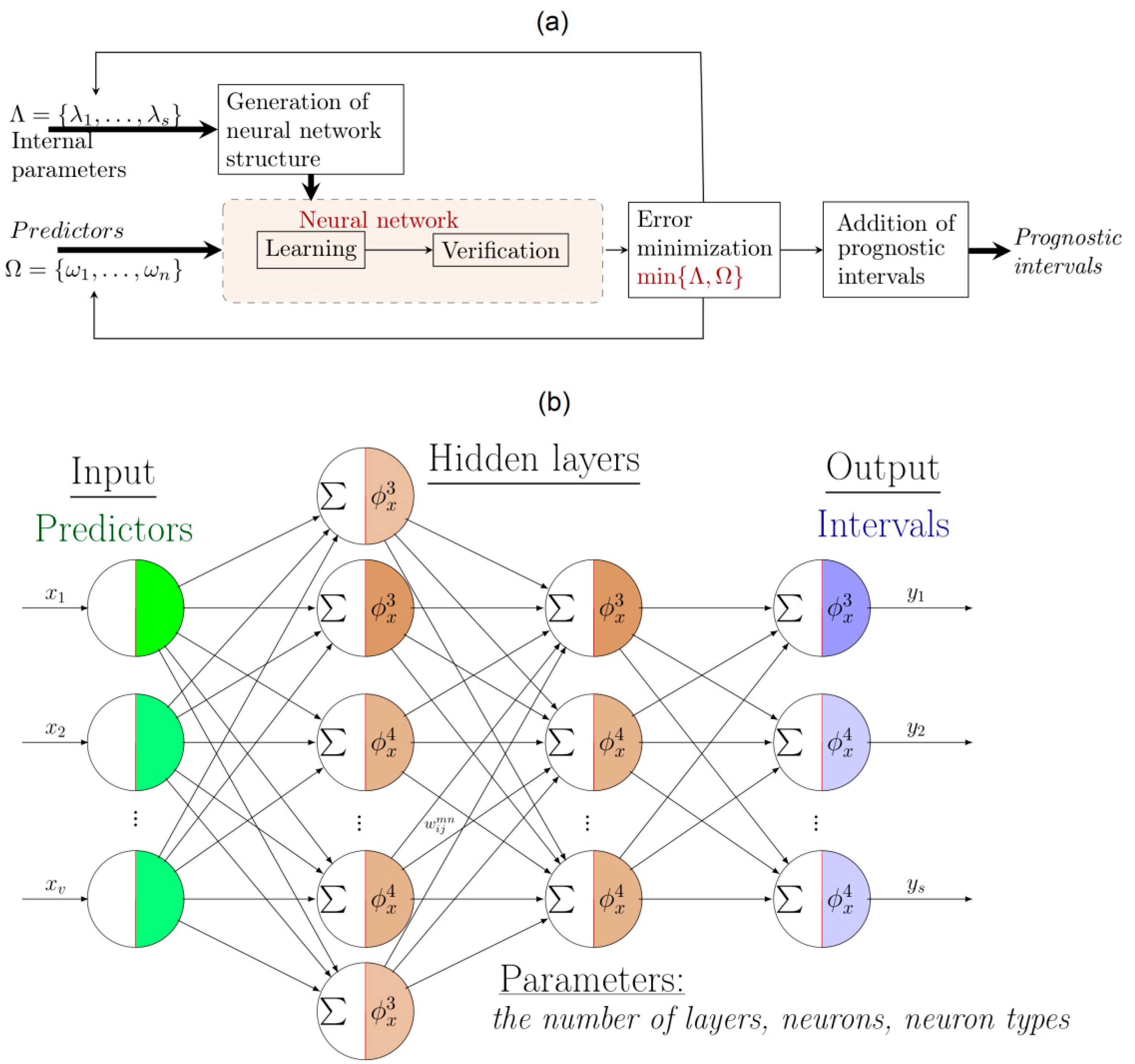
The use of neural networks for prognostic estimations of river flow and temperature conditions makes it possible to obtain more reliable estimates but does not guarantee their unambiguity, which is associated with the choice of the type and form of neural models. Given the complexity of the prognostic problems related to changes in dynamics of the atmospheric circulation and limited knowledge about the influence of cosmic and intraterrestrial factors on it, one should constantly develop new approaches or refine those already known. To generate predictive estimates of effective water inflow into lake, or its components (for example, flows of the Selenga river, Barguzin river, Upper Angara river, southern rivers, and other rivers flowing into the lake), a multivariate neural network (MNN) is implemented in the GeoGIPSAR system. The core of this neural network is developed using the error backpropagation method (
Figure 1b) with an automated setting of the most acceptable parameters based on the testing results on verification samples (
Figure 1a). The MNN parameters are the list and types of input predictors, the number of hidden layers, the number of neurons of various types with various parameters of sigmoidal functions.
A distinction between interval estimates and point ones is that instead of point numerical output indicators, the number of the interval to which the corresponding value belongs is set. The number of intervals into which the entire admissible range of indicators is divided usually varies from 5 to 10. The use of intervals for forecasting the effective inflow into the lake is due to the approximate nature of the accumulated monthly statistics, which are determined by indirect indicators (the statistics have large errors due to the lack of observations on most of the rivers and streams flowing into Lake Baikal).
3. Results
3.1. Monitoring the Actual Indicators of the State of the Atmosphere
As an example of predictive estimates,
Figure 2 shows the maps of deviations of the average indicators of precipitation and temperatures for months 8 and 9 (August–September) for the summer-autumn period of 2020 (a,b); average monthly relative humidity in September, which is anomalous in terms of water content (c), and visualization of rare cyclonic activity related to the geopotential distribution on the isobaric surface of 500 hPa in the catchment area of Lake Baikal (d). It is worth noting that the cyclonic activity of 2020, which led to the excess of the maximum allowable mark of the lake level under normal water conditions, could be recorded using similar maps starting even in the mid-July of this year.
Continuous monitoring of changes in the state of actual atmospheric indicators allows a real-time verification of prognostic indicators and real-time, if necessary, refinement or reformulation of prognostic indicators for the future period. To make macro-estimations of the atmospheric state, it suffices to use the NOAA/NCEP and GPCC re-analyses data with the real-time verification of precipitation and temperature conditions in the studied basin according to the data of the nearest meteorological stations.
3.2. Predictive Estimates Generated by Processing Predictive Ensembles of the Global CFSv2 Model
One can quickly generate similar maps for other indicators for various periods and compare them with the analog years determined by the above method. When processing the set of accumulated prognostic ensembles, which are updated daily by the global climate model CFSv2, maps of distribution probabilities can be generated in advance for various indicators.
Figure 3 shows examples of maps created in September–October 2021 for anomalies of predicted distributions of surface temperatures (a) and precipitation intensities (b) for February 2022; dynamics of changes in the probabilistic prognostic indicators of temperature conditions in the vicinity of Kyakhta (c) in comparison with the minimum, average and maximum daily indicators for 1995–2020. The surface average temperatures in February 2022 show a slight deviation from the norm. Average monthly deviations of precipitation intensity show a slight excess of the norm, except for a small central part of Lake Baikal.
Similar maps of spatial distributions can be quickly generated for other periods (month, decade, week) and other meteorological parameters. The predictive results presented are not conclusive. When significant disturbances appear in the atmosphere, both the distributions of meteorological indicators and the probable trajectories of their dynamics for different areas of the Lake Baikal drainage basin can change.
3.3. MNN-Generated Predictive Estimates
Findings indicate that the reliability of the final result can be increased by synthesizing various MNN models with different sets of predictors and a set of parameters of its structure. The interval estimates are preferable to use compared to specific values, which is associated with the inaccuracy of the initial data. For example, effective inflow to Lake Baikal is estimated through surface inflow, given the groundwater component, evaporation, condensation, and precipitation on the water surface of the lake.
Figure 4 shows an example of predictive interval estimates of the effective inflow of water into Lake Baikal for the 3rd quarter, which were made using MNN based on the predictors in the form of vorticity indices with the maximum correlations found using the absolute values for various atmosphere layers (850, 700, 500 hPa). The lower Figure, for clarity, shows the superimposition of the vector field of average velocities for February 2021. The vorticity indices are calculated for each year of the selected one or several months with the creation of time series and the selection of the most significant ones in correlation with the effective inflow into the lake. Areas with considerable correlations are highlighted in color: negative ones are blue and positive ones are yellow-red. The size of the area for calculating the vorticity index of the atmosphere layer and the threshold values of the correlation coefficients are set by parameters.
The time series of average quarterly inflow (
Figure 4a) is divided into seven intervals (green color denotes an interval with inflow values that are close to the norm). The “+” sign on the learning sample marks centers of intervals after the MNN training. Rectangles (and small diamonds with a probability less than 0.8) on the verification sample mark the results of the trained MNN operation. The above results show an error in the verification sample for no more than one interval (underestimated indicators for 2018–2020). For 2021, the most probable interval according to the results of calculations with the considered MNN model appeared to be slightly below the norm.
A feature of the approach to using neural networks is that for each interval (month, quarter, season), several original models are synthesized with a different set of predictors and internal parameters that satisfy the condition:
where
NSE—the Nash–Sutcliffe coefficient of efficiency [
42];
NM determines the maximum deviation in interval calculus on complex verification samples with the obligatory inclusion of extremely low and extremely high indicators;
—predicted, actual and average intervals on a verification sample of length
T;
— the probability of the predictive value creation for the moment of time
t (
N—the number of intervals for dividing the range of the studied indicator). When training, as a rule, the probability of the maximum value of the interval is much higher than the rest. For refined estimates with the possibility of specifying the redistribution of the probabilities of the initial data at the interval boundaries, it is proposed to use the quantile assessments given in the works [
43,
44].
According to the given condition, only those models are selected (through automated procedures for proposing hypotheses and selecting subsets of predictors based on them) that, at least, do not give a negative indicator NSENM. The maximum value of this indicator is 1, which corresponds to the high efficiency of the model. As we approach the predicted interval, new potential predictors are added that can improve the result. In the case of successful synthesis of several valid models, the final result is determined either by the maximum frequency of the predicted interval, or through another method of interval division of the possible range. Taking into account the specifics of the considered approach, its comparison with many existing ones does not seem correct at this stage of research.
4. Discussion
It is worth noting that the development of a reliable indicator of the prediction interval for the effective inflow into the lake is of great practical value even when divided into only five intervals (extremely low, decreased, normal, increased, and extremely high). The division into a greater number of intervals increases the accuracy of estimates, but their reliability (resistance to various disturbances) may decrease.
The MNN-based methodology proposed in the paper does not allow the guaranteed construction of practically admissible neural network models. The developed algorithms for the predictor selection based on actual indicators from open data of re-analyses make it possible to study many such models with various external verification samples and internal parameters of MNN.
In this regard, we consider it to be promising to use deep learning neural networks, such as convolutional neural networks (CNN) [
45,
46], in the future, which allows finding admissible solutions more efficiently. Currently, we are planning to develop a portable CNN software component with a simple but effective means of its operation, as is implemented for the other components in the GeoGIPSAR system.
The considered approach of using neural networks with the creation of interval estimates is not effective for creating a unified model for forecasting time series in monthly or quarterly time resolutions due to the different scale of indicators. For such a model, it is necessary to use numerical indicators with standard efficiency estimates
NSE,
NRMSE,
RMSE, etc. [
42].
In general, we have proposed a portable, lightweight technology under development for real-time monitoring of the state of the main atmospheric parameters, accumulating, and processing of predictive ensembles of the global CFSv2 model, and making predictive estimations based on MNN with a periodic real-time refinement of prognostic indicators when new climatic data appear.
5. Conclusions
Method proposed for monitoring and making prognostic estimates of atmospheric state parameters in the catchment area of the lake at issue allows their real-time analysis, which can be instrumental to various specialists involved in ecological, hydrological, and water management monitoring of Lake Baikal. The authors’ approach is, first of all, technology and is only the beginning of a complex work of reliable long-term prognostic assessments creation in the catchment basin of Lake Baikal that are acceptable for managing its level regime.
To apply this method in practice, we suggest monthly updating of the analog years, predictive distributions of atmospheric parameters, and monthly average, quarterly average, and average annual indicators of the effective inflow into Lake Baikal with the real-time identification of unlikely events, if any.
Author Contributions
Conceptualization, N.V.A.; Data curation, E.N.O.; Investigation, N.V.A. and T.V.B.; Methodology, N.V.A.; Project administration, V.M.N.; Resources, T.V.B.; Software, E.N.O.; Supervision, V.M.N.; Visualization, E.N.O.; Writing—original draft, N.V.A.; Writing—review & editing, T.V.B. All authors have read and agreed to the published version of the manuscript.
Funding
The work was supported by the grant N° 075-15-2020-787 in the form of a subsidy for a Major scientific project from the Ministry of Science and Higher Education of Russia (project “Fundamentals, methods and technologies for digital monitoring and forecasting of the environmental situation on the Baikal natural territory”).
Institutional Review Board Statement
Not applicable.
Informed Consent Statement
Not applicable.
Conflicts of Interest
The authors declare no conflict of interest.
References
- Törnqvist, R.; Jarsjö, J.; Pietroń, J.; Bring, A.; Rogberg, P.; Asokan, S.M.; Destouni, G. Evolution of the hydro-climate system in the Lake Baikal basin. J. Hydrol. 2014, 519, 1953–1962. [Google Scholar] [CrossRef] [Green Version]
- Hampton, S.E.; Izmest’eva, L.R.; Moore, M.V.; Katz, S.L.; Dennis, B.; Silow, E.A. Sixty years of environmental change in the world’s largest freshwater lake—Lake Baikal, Siberia. Glob. Chang. Biol. 2008, 14, 1947–1958. [Google Scholar] [CrossRef] [Green Version]
- Shimaraev, M.N.; Sizova, L.N.; Troitskaya, E.S.; Kuimova, L.N.; Yakimova, N.I. Ice-thermal Regime of Lake Baikal under Conditions of Modern Warming (1950–2017). Russ. Meteorol. Hydrol. 2019, 44, 679–686. [Google Scholar] [CrossRef]
- Nikitin, V.M.; Abasov, N.V.; Bychkov, I.V.; Osipchuk, E.N. Level Regime of Lake Baikal: Problems and Contradictions. Geogr. Nat. Resour. 2019, 40, 353–361. [Google Scholar] [CrossRef]
- Abasov, N.V.; Bolgov, M.; Nikitin, V.M.; Osipchuk, E.N. Level regime regulation in Lake Baikal. Water Resour. 2017, 44, 537–546. [Google Scholar] [CrossRef]
- Saha, S.; Moorthi, S.; Wu, X.; Wang, J.; Nadiga, S.; Tripp, P.; Behringer, D.; Hou, Y.-T.; Chuang, H.-Y.; Iredell, M.; et al. The NCEP climate forecast system version 2. J. Clim. 2014, 27, 2185–2208. [Google Scholar] [CrossRef]
- Yuan, X.; Wood, E.; Luo, L.; Pan, M. A first look at climate forecast system version 2 (CFSv2) for hydrological seasonal prediction. Hydrol. Land Surf. Stud. 2011, 38. [Google Scholar] [CrossRef] [Green Version]
- Rai, A.; Saha, S.K. Evaluation of energy fluxes in the NCEP climate forecast system version 2.0 (CFSv2). Clim. Dyn. 2018, 50, 101–114. [Google Scholar] [CrossRef]
- Hourdin, F.; Mauritsen, T.; Gettelman, A.; Golaz, J.-C.; Balaji, V.; Duan, Q.; Folini, D.; Ji, D.; Klocke, D.; Qian, Y.; et al. The Art and Science of Climate Model Tuning. Bull. Am. Meteorol. Soc. 2017, 98, 589–602. [Google Scholar] [CrossRef]
- Berezhnykh, T.; Abasov, N. The increasing role of long-term forecasting of natural factors in energy system management. Int. J. Glob. Energy Issues 2003, 20, 353–363. [Google Scholar] [CrossRef]
- ERA5/ECMWF Data. Available online: https://www.ecmwf.int/en/forecasts/datasets/reanalysis-datasets/era5 (accessed on 10 November 2021).
- ECMWF ERA-40 Data. Available online: https://www.cgd.ucar.edu/cas/catalog/reanalysis/ecmwf/era40 (accessed on 10 November 2021).
- NOAA Reanalysis Data. Available online: ftp://ftp.cdc.noaa.gov/Datasets/ncep.reanalysis.dailyavgs (accessed on 10 November 2021).
- A Global Map of Wind, Weather, and Ocean Condition. Available online: https://earth.nullschool.net (accessed on 10 November 2021).
- Windy: Wind Map and Weather Forecast. Available online: https://www.windy.com (accessed on 10 November 2021).
- Ventusky—Wind, Rain, and Temperature Maps. Available online: https://www.ventusky.com (accessed on 10 November 2021).
- Global Precipitation Climatology Centre (GPCC). Available online: https://www.dwd.de/EN/ourservices/gpcc/gpcc.html (accessed on 10 November 2021).
- Schneider, U.; Becker, A.; Finger, P.; Rustemeier, E.; Ziese, M. GPCC Monitoring Product: Near Real-Time Monthly Land-Surface Precipitation from Rain-Gauges Based on SYNOP and CLIMAT Data; Global Precipitation Climatology Centre: Berlin, Germany, 2020. [Google Scholar]
- Schamm, K.; Ziese, M.; Becker, A.; Finger, P.; Meyer-Christoffer, A.; Schneider, U.; Schröder, M.; Stender, P. Global gridded precipitation over land: A description of the new GPCC First Guess Daily product. Earth Syst. Sci. Data 2014, 6, 49–60. [Google Scholar] [CrossRef] [Green Version]
- Schneider, U.; Finger, P.; Meyer-Christoffer, A.; Rustemeier, E.; Ziese, M.; Becker, A. Evaluating the hydrological cycle over land using the newly-corrected precipitation climatology from the global precipitation climatology centre (GPCC). Atmosphere 2017, 8, 52. [Google Scholar] [CrossRef] [Green Version]
- Schneider, U.; Becker, A.; Finger, P.; Meyer-Christoffer, A.; Ziese, M.; Rudolf, B. GPCC’s new land surface precipitation cli-matology based on quality-controlled in situ data and its role in quantifying the global water cycle. Theor. Appl. Climatol. 2014, 115, 15–40. [Google Scholar] [CrossRef] [Green Version]
- Becker, A.; Finger, P.; Meyer-Christoffer, A.; Rudolf, B.; Schamm, K.; Schneider, U.; Ziese, M. A description of the global land-surface precipitation data products of the global precipitation climatology centre with sample applications including centennial (trend) analysis from 1901–present. Earth Syst. Sci. Data 2013, 5, 71–99. [Google Scholar] [CrossRef] [Green Version]
- Dedicated Data for Climate Research. Available online: http://aisori-m.meteo.ru/waisori/index0.xhtml (accessed on 10 November 2021).
- Operational Data of the Site “Weather and Climate”. Available online: http://www.pogodaiklimat.ru (accessed on 10 November 2021).
- Berezhnykh, T.V.; Marchenko, O.Y.; Abasov, N.V.; Mordvinov, V.I. Changes in the summertime atmospheric circulation over East Asia and formation of long-lasting low-water periods within the Selenga river basin. Geogr. Nat. Resour. 2012, 33, 223–229. [Google Scholar] [CrossRef]
- Abasov, N.V.; Berezhnykh, T.V.; Vetrova, V.V.; Marchenko, O.Y.; Osipchuk, E.N. Analysis and forecasting of the Baikal region hydropower potential under the conditions of varied climate. In Risks and Opportunities of the Energy Sector in East Siberia and the Russian Far East: For Better Risk Management and Sustainable Energy Development; Ko, S., Lee, K.W., Eds.; Lit Verlang Dr. W. Hopf: Berlin, Germany, 2012; pp. 173–186. [Google Scholar]
- Srikanth, B.; Selvarani, G.A.; Sahoo, B.B. Forecasting monthly discharge using machine learning techniques. Int. Res. J. Multidiscip. Technovation 2019, 1, 1–6. [Google Scholar] [CrossRef]
- Marques, C.; Ferreira, J.; Rocha, A.; Castanheira, J.M.; Melo-Gonçalves, P.; Vaz, N.; Dias, J. Singular spectrum analysis and forecasting of hydrological time series. Phys. Chem. Earth Parts A/B/C 2006, 31, 1172–1179. [Google Scholar] [CrossRef]
- Pai, P.-F.; Lin, K.-P.; Lin, C.-S.; Chang, P.-T. Time series forecasting by a seasonal support vector regression model. Expert Syst. Appl. 2010, 37, 4261–4265. [Google Scholar] [CrossRef]
- Burakov, D.; Adamovich, A. Long-term forecasts of water inflow to reservoirs of the Yenisei hydroelectric power plants with the use of a mathematical model. Meteorol. Hydrol. 2006, 1, 74–82. [Google Scholar]
- Londhe, S.; Charhate, S. Comparison of data-driven modelling techniques for river flow forecasting. Hydrol. Sci. J. 2010, 55, 1163–1174. [Google Scholar] [CrossRef]
- Huang, S.; Chang, J.; Huang, Q.; Yutong, C. Monthly streamflow prediction using modified emd-based support vector ma-chine. J. Hydrol. 2014, 511, 764–775. [Google Scholar] [CrossRef]
- Hadiyan, P.P.; Moeini, R.; Ehsanzadeh, E. Application of static and dynamic artificial neural networks for forecasting inflow discharges, case study: Sefidroud dam reservoir. Sustain. Comput. Inform. Syst. 2020, 27, 100401. [Google Scholar] [CrossRef]
- Cheng, C.T.; Lin, J.Y.; Sun, Y.G.; Chau, K. Long-term prediction of discharges in manwan hydropower using adaptive-network-based fuzzy inference systems models. Lecture Notes Comput. Sci. 2005, 3612, 434. [Google Scholar]
- Feilat, E.A.; Al-Sha’abi, D.T.; Momani, M. Long-term load forecasting using neural network approach for Jordan’s power system. Eng. Press 2017, 1, 43–50. [Google Scholar]
- Gelfan, A.; Moreydo, V.; Motovilov, Y.; Solomatine, D.P. Long-term ensemble forecast of snowmelt inflow into the cheboksary reservoir under two different weather scenarios. Hydrol. Earth Syst. Sci. 2018, 22, 2073–2089. [Google Scholar] [CrossRef] [Green Version]
- Xu, J.; Zhang, Q.; Liu, S.; Zhang, S.; Jin, S.; Li, D.; Wu, X.; Liu, X.; Li, T.; Li, H. Ensemble learning of daily river discharge modeling for two watersheds with different climates. Atmos. Sci. Lett. 2020, 21, e1000. [Google Scholar] [CrossRef]
- Adhikari, A.; Patra, K.C.; Adhikari, N. Machine learning approach for discharge estimation in compound channels. ISH J. Hydraul. Eng. 2018, 27, 100–109. [Google Scholar] [CrossRef]
- Meshram, S.G.; Meshram, C.; Santos, C.A.G.; Benzougagh, B.; Khedher, K.M. Streamflow prediction based on artificial intelligence techniques. Iran. J. Sci. Technol. Trans. Civ. Eng. 2021, 1–11. [Google Scholar] [CrossRef]
- Lima, G.; Scofield, G. Feasibility study on the operational use of neural networks in a flash flood early warning system. RBRH 2021, 26. [Google Scholar] [CrossRef]
- Hovmöller, E. The trough-and-ridge diagram. Tellus 1949, 1, 62–66. [Google Scholar] [CrossRef]
- Zhou, X.; Huang, G.; Piwowar, J.; Fan, Y.; Wang, X.; Li, Z.; Cheng, G. Hydrologic impacts of ensemble-RCM-projected climate changes in the athabasca river basin, canada. J. Hydrometeorol. 2018, 19, 1953–1971. [Google Scholar] [CrossRef] [Green Version]
- Mehdiyev, N.; Enke, D.; Fettke, P.; Loos, P. Evaluating forecasting methods by considering different accuracy measures. Procedia Comput. Sci. 2016, 95, 264–271. [Google Scholar] [CrossRef] [Green Version]
- de la Torre, J.; Puig, D.; Valls, A. Weighted kappa loss function for multi-class classification of ordinal data in deep learning. Pattern Recognit. Lett. 2018, 105, 144–154. [Google Scholar] [CrossRef]
- Benidis, K.; Rangapuram, S.S.; Flunkert, V.; Wang, B.; Maddix, D.; Turkmen, C.; Gasthaus, J.; Bohlke-Schneider, M.; Salinas, D.; Stella, L.; et al. Neural Forecasting: Introduction and Literature Overview; Amazon Research: Seattle, WA, USA, 2020. [Google Scholar]
- Ghosh, A.; Sufian, A.; Sultana, F.; Chakrabarti, A.; De, D. Fundamental Concepts of Convolutional Neural Network. In Recent Trends and Advances in Artificial Intelligence and Internet of Things; Springer: Cham, Switzerland, 2020; pp. 519–567. [Google Scholar] [CrossRef]
| Publisher’s Note: MDPI stays neutral with regard to jurisdictional claims in published maps and institutional affiliations. |
© 2021 by the authors. Licensee MDPI, Basel, Switzerland. This article is an open access article distributed under the terms and conditions of the Creative Commons Attribution (CC BY) license (https://creativecommons.org/licenses/by/4.0/).


