Article

Suitability of Different Methods for Measuring Black Carbon Emissions from Marine Engines

1
VTT Technical Research Centre of Finland, P.O. Box 1000, 02044 Espoo, Finland
2
Aerosol Physics Laboratory, Physics Unit, Faculty of Engineering and Natural Sciences, Tampere University, 33100 Tampere, Finland
3
Atmospheric Composition Research, Finnish Meteorological Institute, P.O. Box 503, 00101 Helsinki, Finland
4
DMPE, ONERA, Université Paris Saclay, CEDEX, 91123 Palaiseau, France
5
Department of Environmental and Biological Sciences, University of Eastern Finland, 70210 Kuopio, Finland
*
Author to whom correspondence should be addressed.
Atmosphere 2022, 13(1), 31; https://doi.org/10.3390/atmos13010031
Submission received: 1 November 2021 / Revised: 17 December 2021 / Accepted: 20 December 2021 / Published: 26 December 2021
(This article belongs to the Topic Climate Change and Environmental Sustainability)

Abstract

:
Black carbon (BC) emissions intensify global warming and are linked to adverse health effects. The International Maritime Organization (IMO) considers the impact of BC emissions from international shipping. A prerequisite for the anticipated limits to BC emissions from marine engines is a reliable measurement method. The three candidate methods (photoacoustic spectroscopy (PAS), laser-induced incandescence (LII), and filter smoke number (FSN)) selected by the IMO were evaluated with extensive ship exhaust matrices obtained by different fuels, engines, and emission control devices. A few instruments targeted for atmospheric measurements were included as well. The BC concentrations were close to each other with the smoke meters (AVL 415S and 415SE), PAS (AVL MSS), LII (Artium-300), MAAP 5012, aethalometers (Magee AE-33 and AE-42), and EC (TOA). In most cases, the standard deviation between instruments was in the range of 5–15% at BC concentrations below 30 mg Sm−3. Some differences in the BC concentrations measured with these instruments were potentially related to the ratio of light-absorbing compounds to sulphates or to particle sizes and morphologies. In addition, calibrations, sampling, and correction of thermophoretic loss of BC explained differences in the BC results. However, overall differences in the BC results obtained with three candidate methods selected by the IMO were low despite challenging exhaust compositions from marine diesel engines. Findings will inform decision making on BC emission control from marine engines.

1. Introduction

Global warming is enhanced by black carbon (BC) emissions directly through increased radiative forcing of atmosphere and indirectly through ice melting through deposition of BC on ice and snow, which is particularly detrimental in the Arctic, along with increasing shipping [1,2,3,4]. The contribution of shipping in global anthropogenic greenhouse gas emissions was 2.89% in 2018 [1], and climate-warming BC emissions from shipping represent 7% of total shipping CO2-equivalent emissions on a 100-year timescale [5,6]. Besides global warming potential, BC, as a part of particulate matter (PM) emissions, is linked to adverse health effects [7,8]. The International Maritime Organization (IMO) has worked on consideration of the impact on the Arctic of emissions of BC from international shipping since 2011 (the 62nd meeting of the Marine Environment Protection Committee (MEPC 62)). The work progressed in 2015 (MEPC 68) by agreeing on the definition of BC for international shipping as defined by Bond et al. [9], and in 2018 by selecting the three candidate methods for BC measurements: photoacoustic spectroscopy (PAS), laser-induced incandescence (LII), and filter smoke number (FSN) (the 5th meeting of the Sub-Committee on Pollution Prevention and Response (PPR 5)).
Specific methods are designed for measuring BC from different sources, and none of the methods alone is optimal for measuring BC from all sources due to significant mismatch of the measurement ranges of the instruments with the BC concentrations and the chemical composition of gas and aerosol matrices [9,10,11,12]. Techniques using PAS, LII, and FSN principles are designed for measuring BC from engine exhaust, although they could also be used for measuring absorbing aerosols from other sources. Light absorption smoke meters (referred to as the FSN method by IMO) are the traditional method for engine exhaust measurements, while PAS and LII methods are new approaches. Techniques designed for characterising BC from ambient air include, for example, optical methods such as multi-angle absorption photometer (MAAP) and aethalometers (AE) [13,14]. Elemental carbon (EC) measured with the thermal-optical (TOA) method from filter samples is by definition not commensurable with the optically measured BC. Additionally, TOA analysis is challenging when using residual fuels in marine diesel engines due to the asphaltene and metal content of PM [15]. The correlation between light-absorption-based BC and thermoanalytically measured EC are discussed by, for example, Pöschl [16].
Each BC measurement method has its limitations related to the operative definitions of the carbonaceous particles [11,14,17]. The optical BC measurement methods are sensitive to interferences by aerosol species affecting the light absorption coefficient and the mass absorption coefficient (MAC), which are needed for converting the light absorption into a BC mass concentration [9,16,17,18,19]. Additionally, most filter-based techniques suffer from artefacts due to scattering caused by the filter fibres and aerosols embedded in the filter (increasing optical path, reflectance) and the filter-loading effect of aerosols accumulated on the filter (reducing optical path) [9,18]. The non-BC light-absorbing aerosol species include brown carbon (BrC), mineral dust [17,20,21,22,23], and also the sulphur content of aerosol, which may have cross-interferences with the light-absorbing properties of BC. Brownish, light-absorbing organic compounds include, for example, polyaromatic hydrocarbons (PAHs). The difference between BC and BrC is not sharply defined, and their differentiation by measurements is challenging [20,23,24,25,26]. BC absorbs light predominantly in the mid-visible wavelength, while BrC contributes in shorter wavelengths, and shows stronger wavelength-dependence than BC [17,27,28,29]. The absorption Ångström exponent (AAE) is determined by instruments using several wavelengths, and it describes the spectral dependence of light absorption by aerosols. Hence, AAE is valuable for source apportionment studies [24,27,28,29,30,31,32]. AAE is low (1.0–1.5) for BC, while AAE values can be high for aerosol containing absorbing organic carbon [20,21] and mineral dust [22]. To be quantitative, the share of non-BC absorbers needs to be high [33]. Some compounds that are condensed in BC, such as semi-volatile organic compounds and water vapour, may enhance absorption by 30–50% via the lensing effect [12]. A thicker coating of particles in an aged aerosol through the formation of secondary organic or inorganic aerosols may lead to overestimated BC [10,11,12,34,35]. Small aerosol particles also absorb more at near-UV than at longer wavelengths, but the effect of particle size on optical measurements of BC is not completely understood. Interferences of non-BC light-absorbing compounds are suggested to be at their minimum at a detection wavelength in the region from 600 nm to 700 nm [14].
Instruments using the filter-based light absorption principle include, for example, smoke meters (SM), MAAP, and aethalometers. The SM instruments measure light absorption by the change in the optical reflectance of visible light (peak at 550–570 nm) from a loaded filter relative to a clean filter. Measured reflectances are converted to FSN and further to BC concentrations as standardised conformity to ISO 10054 and ISO 8178-1. MAAP measures the relative change in optical transmission and reflectance of scattered light as particles are collected on a filter at a wavelength of 670 nm with multiple detectors simultaneously [36]. Since MAAP detects transmitted and backscattered light at two angles, instrumental aerosol-composition-dependent artefacts are reduced [14]. Aethalometers resemble MAAP, but they do not measure scattered light and hence do not correct instrumental artefacts caused by scattering. Aethalometers use several wavelengths, from which absorption at 880 nm is typically interpreted as BC. Aethalometer types using a double detection system minimise the filter-loading effect [37], viz. overestimation of BC concentration on a fresh filter and underestimation on a loaded filter [38], while the most correct concentrations are on lightly loaded filters [11]. PAS and LII are filter-free, in situ methods to measure BC, hence filter-related artefacts are avoided. These “zero background” methods are also more sensitive than the differential methods [39,40]. In the PAS principle, a modulated laser beam causes periodic temperature and pressure changes in the surrounding gas sample, and a sound pressure wave is detected by a microphone. [41]. Multi-wavelength PAS is an option [39,40]. The common PAS instrument, the AVL Micro Soot Sensor (MSS), uses 808 nm to determine absorption by BC [42,43], and correlation between PAS signal and BC mass is calibrated using a combustion aerosol standard analysed by the EC(TOA) [42]. Consequently, the interferences in the EC(TOA) analysis, for example, due to asphaltenes and metals potentially present in marine engine exhaust [15,43], affect calibration of the PAS. MSS(PAS) is a standard reference instrument for certification of aircraft engines (SAE E-31 AIR 6241). LII measures the thermal emission emitted from soot particles heated by the Nd:YAG pulsed laser (usually 1064 nm) to temperatures in the range from 2500 K to 4500 K. The laser fluence is set to a value, which heats the soot particles below their sublimation threshold values (4000 K for BC) [44,45,46]. The LII is by default insensitive to liquid particles and metal salts, which vaporise during the heating, although some impact of OC coating of soot in LII response has been reported [47,48]. The size of the soot agglomerates may have an impact on the LII response, which needs to be taken into account in calibration of the LII signal to the BC concentration [49].
All BC measurement technologies, filter- or non-filter-based, are suspected to suffer from interference, at least to some extent. In addition, methods use different reference materials for calibration [50]. The artefacts, combined with lack of a traceable and universally agreed upon BC reference material or methods, complicates setting regulations on BC emissions. Correlations between methods are typically decent, but regression slopes may vary [12,25], and intercomparison studies have shown substantial differences in BC concentrations between thermal and optical methods [51,52,53,54,55,56]. Instrument type, exhaust sampling, dilution and sample treatment procedures affect the BC results, which are topics for standardisation of measurements. Special considerations are needed for the BC measurements from marine engine exhaust due to its high temperature, potential content of sulphuric acid, sulphates (SO42) and bound water, metals, and BrC, along with a wide range of particle sizes. Sulphur content of marine fuels will remain high, for example, in scrubber-equipped ships even after the introduction of the 0.5% global sulphur limit for marine fuels in 2020. The sulphates from ship emissions induce a cooling effect on the climate by reducing the absorption of visible light at longer wavelengths [57].
In this study, the suitability of three candidate methods (PAS, LII, and FSN) selected by the IMO for measuring BC emissions from marine engines was studied and discussed in view of controlling BC emissions from marine engines in the future. The measurement setup included instruments representing the FSN method (AVL 415S and AVL 415SE), PAS method (AVL MSS 483), LII method (Artium 300), and additionally MAAP, aethalometers, and TOA. Three campaigns covered measurements on-board a ship from two modern medium-speed diesel (MSD) engines, one equipped with selective catalytic reduction (SCR) and SOx scrubber, the other one equipped with scrubber only, using two fuels (0.6%S and 0.1%S). In laboratory, emissions from an MSD engine fuelled with three fossil fuels having sulphur contents up to 2.5 weight percent (wt%) and a 30% blend of biofuel fatty acid component (BioFA), while a modern high-speed diesel (HSD) engine fuelled with two sulphur-free fuels with different aromatic contents were characterised. The results from exceptionally wide real-life exhaust matrices from campaigns with different fuels, engines, and emission control devices enabled in-depth analysis of the differences between instruments measuring the BC emissions. New findings on the behaviour of the instruments and parameters to be considered (e.g., (AAExBC):SO4 and fuel properties) are presented. Furthermore, sampling issues are presented and discussed, since representative sampling is a prerequisite for reliable results. In this respect, correction of the thermophoretic loss of BC in the transfer line when sampling hot and humid engine exhaust potentially explains some differences in the results between instruments. All in all, experimental campaigns with various fuels, engines, and emission control devices provided extensive ship exhaust matrices to study the behaviour of the BC-measuring instruments, as well as discussion of significant parameters and sampling issues to evaluate the suitability of the studied measurement principles for marine engine measurements and regulations.

2. Materials and Methods

2.1. Measurement Campaigns

Three marine engine emission measurement campaigns, A, B, and C, were carried out in a laboratory and on-board ship (Table 1, details in the Supplementary Material Section S2 with refs [51,58,59,60,61,62]). In campaign A, laboratory tests were conducted with an MSD engine in the size range of auxiliary power engines in ships, a 1.6 MW Wärtsilä Vasa 4R32 LN (Wärtsilä, Finland) (Table S2 in the Supplementary Materials) at two engine loads (75% and 25%) corresponding to the open sea and near-harbour engine-loading conditions. In campaign B, on-board measurements were conducted from two modern medium-speed diesel engines (MSD1, MSD2), with one engine equipped with the SCR and scrubber, and the other engine with the scrubber only, at engine loads of 75% and 40%. The third campaign, C, was carried out with a high-speed diesel engine (HSD) in a laboratory. Engine characteristics are presented in Tables S1, S2 and S5 in the Supplementary Materials.
In campaign A, the three fuels used represented different sulphur contents (2.5%S, 0.5%S, and 0.1%S fuels; abbreviation %S means the sulphur content of fuel in percentage), and the fourth fuel contained 30% fatty-acid-type biocomponent (Bio-FA) (Table S3 in the Supplementary Materials). The fuels were characterised and were observed to have different compositions, including different aromatic, asphaltene, and ash content. PAHs(di+) content in 0.1%S fuel was 10.8% and ash content was <0.005 wt%, while BioFA fuel had PAH(di+) content of only 2.8 wt%. Residual fuels (0.5%S and 2.5%S) contained heavy asphaltenes (5.7 wt% and 28.3 wt%) and ash (0.038 wt% and 0.094 wt%). In campaign B, HFO (0.6%S) and MGO (0.1%S) fuels were used, and in campaign C, two sulphur-free diesel fuels, one that was aromatic-free diesel fuel (Ar-0) and another that was high-aromatic diesel fuel (Ar-20), were used.
Methods and setups are described in Sections S1 and S2 in the Supplementary Materials. Numerical results of the gaseous emissions (CO, HC, NOx, CO2) and the particle-related emissions (PM and its composition, BC) are presented in Section S5 in the Supplementary Materials.

2.2. Instrumentation

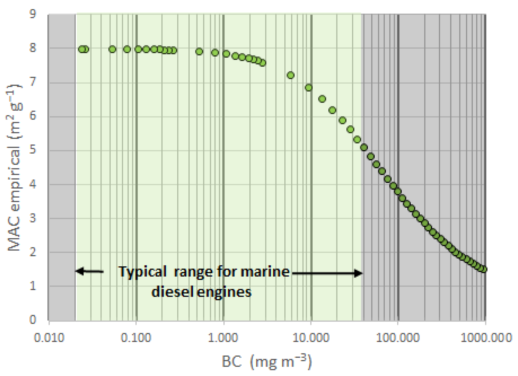
2.2.1. Light Absorption Smoke Meters (FSN Method) and Calculated MACBC

The SM instruments used were AVL 415S and AVL 415SE (AVL List GmbH, Austria), which measure the raw exhaust gas without the need for exhaust dilution. The BC measurement range of instruments was from 20 µg/m3 to 32 g/m3. SM model AVL415SE introduced “Shop Air Purging” to improve the cleaning of instruments when using residual fuels. Conversion of FSN to the BC concentration was conducted by the manufacturer’s equation, which takes into account thermophoretic losses (AVL List GmbH, Equation (S2) and Figure S1 in the Supplementary Materials). Methodology and conversion of measured reflectances to FSN and further to BC concentrations is standardised conformity to ISO 10054 and ISO 8178-1. SM(FSN) measured three replicates in one minute. The output concentrations at 100 kPa and 298.15 K were converted to reference conditions at 101.3 kPa and 273.15 K (abbreviated mg Sm−3). Details are presented in Appendix B and Section S1.1 in the Supplementary Materials with [9,42,63,64,65].
Light absorption SM instruments measure light absorption by the change in optical reflectance of visible light from a loaded filter relative to a clean filter. The mass absorption coefficient (MACBC) was calculated for these SM instruments with source information of (a) the standard ratio of Af /Vs = 2.47 m−1, where Vs is sample volume and Af is an effective cross-section area of a filter as specified in ISO 10054, and (b) reflectometer voltages (R) converted to a blackening (absorbance) fraction (1-Rsample/Rclean) scaled to FSN/10 and further to BC concentrations (details in the Section S1.1 in the Supplementary Materials). The thermophoretic loss correction of 15% was based on average parameters of the engine tests. Figure 1 shows that MACBC at 550–570 nm depends on BC concentrations, being in the range of 6–8 m2 g−1 at BC concentrations below 20 mg Sm−3, while gradually decreasing at higher BC concentrations. ISO 10054 defines that light source and receiver shall have a peak spectral response in the region from 550 to 570 nm.

2.2.2. AVL Micro Soot Sensor

The AVL Micro Soot Sensor (MSS) (AVL List GmbH, Austria) used in this study measures with the photo acoustic principle [30,42,43]. The AVL MSS instrument has its own diluter. The 808 nm light is absorbed by the particles. The AVL MSS provides a continuous online measurement of BC concentration at a rate of up to 10 Hz. One second intervals were used in this study. MSS is a standard reference instrument for the certification of aircraft engines (SAE E-31 AIR 6241, ARP6320). The measurement range of AVL MSS is from 1 µg/m3 to 50 mg/m3. MSS settings are presented in Appendix A, Table A1, other details in Appendix B and in Section S1.2 in the Supplementary Materials with [42,43].
Thermophoretic losses in the transfer line were corrected manually in the AVL MSS data. For the MSD engine in the laboratory campaign, the correction factor (cf) was 1.17 at high load and 1.14 at low load. In the on-board MSD measurements, the cf was 1.11–1.15, while for cold exhaust after the scrubber, the cf was 1.0. In the HSD measurements, the cf was 1.0–1.12, depending on engine load. AVL MSS output concentrations are corrected by firmware to 101.3 kPa and 273.15 K.

2.2.3. LII instrument Artium 300

The LII instrument used in the measurements was the Artium 300 instrument (hereinafter LII 300) (Artium Technologies, Canada) (details in Appendix B and in Section S1.3 in the Supplementary Materials). Emissions recorded from LII 300 signals can be used for determination of the mass concentration, volume concentration, active surface area, and primary particle diameter of soot particle emissions. LII 300 can measure at a rate of up to 10 Hz [44,45,46]. The LII 300 instrument used in this study is accepted in the aircraft engine certification procedure. LII 300 was calibrated using emissions from a Rolls Royce Gnome engine (Rolls Royce, United Kingdom), and its limit of detection (LoD) was 2 µg/m3, although an instrument could be calibrated down to LoD of 0.2 µg/m3 in the high-sensitivity mode. LII 300 data was manually corrected for the thermophoretic losses. See Appendix A, Table A1, and Appendix B.

2.2.4. MAAP and Aethalometers

The multiangle absorption photometer, MAAP 5012 (Thermo Fisher Scientific, Franklin, Massachusetts, United States), which is used in these measurements, measures the relative change in optical transmission as particles are collected on a filter combined with a measurement of reflectance of scattered light at a wavelength of 670 nm with multiple detectors simultaneously [36]. Calculation is based on a specific absorption of BC at a certain wavelength. MAAP provides continuous measurement at time intervals of at least one minute. A high dilution ratio is needed when measuring diesel exhaust, as the instrument is designed for ambient measurements. The BC measurement range of MAAP can be up to 60 µg/m3 with certain measurement parameters, but BC concentrations may already be underestimated at 9 µg/m3; see Appendix B and Section S1.4 in the Supplementary Materials with [18,66].
Aethalometers, AE42 and a newer model AE33 (Magee Scientific, Berkeley, CA, United States), measure the change in absorption of transmitted light due to collection of aerosol deposit on reinforced quartz fibre tape, which advances automatically when its loading threshold is reached [37]. In both aethalometers, measurement of absorption at 880 nm is interpreted as BC. AE33 uses seven wavelengths: 370 (UV), 470 (blue), 520 (green), 590 (yellow), 660 (red), 880 (IR-1), and 950 nm (IR-2), and a DUALSPOT™ technology alleviates “spot loading effects” [38]. These aethalometers provide continuous BC measurements at one minute or one second intervals. The measurement range of AE33 is 0.01–100 µg/m3. The output concentrations are at prevailing temperature and pressure, and they were converted to reference conditions (101.3 kPa, 273.15 K). See Appendix A, Table A1, Table A3, and Section S1.5 in the Supplementary Materials with [11,37,38,67,68].

2.2.5. Thermal-Optical Analysis

The quartz filters used for TOA analyses were Munktell MK360 (Munktell, Sweden) (campaign A) and Pall Tissuequartz (Pall Corporation, Port Washington, NY, United States) (campaigns B and C). These filters were pre-cleaned at 400 °C for two hours and stabilised. Loaded filters were stored in the freezer. See sampling details in Section 2.2.6. For elemental and organic carbon (EC/OC) analysis via the TOA method [69], the Sunset Laboratories Inc’s analyser model 4L was used. Temperature and gas atmosphere is adjusted while continuously measuring the transmission of a laser through the sample matrix. In the second phase, the sample is cooled, O2/He is introduced, and the temperature is raised again. Carbon is oxidised to CO2, which is then converted to methane and detected by the FID. The organic compounds pyrolytically converted to EC are compensated for by continuous measurement of the transmission of a laser. Based on the FID response and laser transmission data, the quantities of OC and EC in the sample are calculated. Methane and saccharose were used for calibration. The temperature program was EUSAAR2 (EN 16909) with peak temperature of 650 °C in the He phase to decrease the risk of premature evolution of EC and to minimise pyrolysis [55], which are risks for the PM samples from marine engines using residual fuels contained oxygen, sulphates, metal salts, and heavy OC. In addition to selection of the temperature program (EUSAAR2) to alleviates these artefacts, the most challenging samples were extracted with water and organic solvents (described in [15]) to remove disturbing constituents before TOA analyses that were parallel to TOA analyses of the untreated samples. The final concentrations are presented in reference conditions (101.3 kPa, 273.15 K).

2.2.6. Dilution, Particulate Matter (PM) Samples for TOA, and PM Characterisation

In both MSD engine campaigns, optimal dilution conditions were used for each BC measurement instrument, and hence sampling for different instruments was not the same. The MSS(PAS) and LII 300 measured at high and low dilution ratios (DRs), while SMs (FSNs) were measured from raw exhaust, and the PM for the TOA analysis was obtained with low DR (Appendix A, Table A1). PM for TOA and chemical characterisation was collected with ISO 8178 partial flow dilution with AVL SmartSampler (AVL List GmbH, Austria) without cyclone or hat, hence also collecting large particles. PM samples were collected using the DR of 8 (ISO 8178 limit: DR > 4), the temperature on the filter face below 52 °C (requirement 42–52 °C), and a face velocity of 37 cm/s on o.d. 70 mm filters (requirement 35–100 cm/s, 2017 version 90–100 cm/s). Transfer line heating was set to approximately 250 °C, except for 70 °C for AVL SM according to the manufacturers’ setting. The sampling probe was heated in the measurements after the scrubber to avoid conducting any possible droplets in instruments, and also before the scrubber to treat the sample in the same way as in the after-scrubber sampling. The first-stage diluters were heated.
PM samples were collected with Pallflex TX40HI20-WW filters (o.d. 70 mm) (Pall Corporation, Port Washington, New York, United States) for anion and PAH analyses. Elemental analysis was conducted from PM sample collected on quartz filters by extraction in a micro-oven by using nitric acid and hydrofluoric acid (EN 14385) and analysis by using inductively coupled plasma mass spectrometry (ICP-MS). Anions, including sulphates, were analysed by electrophoresis from water/isopropanol extracts. Water bound in sulphates was calculated according to SAE J1936 (standard of Society of Automotive Engineers), assuming relative humidity of 50% for other fuels than 2.5%S, for which a lower factor was used to adjust the composition with the PM’s mass. PAHs were analysed from toluene extracts of PM. Additionally, in-stack PM samples were collected according to standard EN 13284-1.
CO, HC, and NOx emissions were measured with analysers meeting the ISO 8178 requirements: THC by heated flame ionisation detector, NOx by heated chemiluminescence, and CO and CO2 by nondispersive infrared. O2 was measured with paramagnetic cell. More than 10 gaseous compounds were measured online at 20 s intervals using Fourier transformation infrared (FTIR) equipment (Gasmet DX-4000, Gasmet Technologies, Finland). Additionally, many parameters were recorded, including engine, fuel and exhaust, and cooling and lubrication parameters.

3. Results and Discussion

3.1. Statistical Analysis of BC Results from Different Instruments

3.1.1. Baseline for Analysis

In three measurement campaigns covering different engines, fuels, and after-treatment technologies, some instruments indicated lower and the others higher BC concentrations relative to one another (Appendix A, Table A1). None of the BC measurement principles used today are deemed to unambiguously measure true BC concentrations, particularly from challenging exhaust from marine diesel engines using residual fuels. EC is well-defined for clean diesel combustion, but not for engine exhaust containing high concentrations of, for example, sulphuric acid and metal salts, heavy organic compounds, and oxygen. Hence, the BC results from the individual instruments were compared with average results obtained with SM(SFN), MSS(PAS), MAAP, EC(TOA), and LII. The instrument selection in the three campaigns is considered suitable for this analysis, since the selection covers many different principles, including MAAP, taking account of both absorption and scattering. Using average BC results from different instruments as baseline in the analysis provides a technology-neutral approach without priority for any of the instruments.

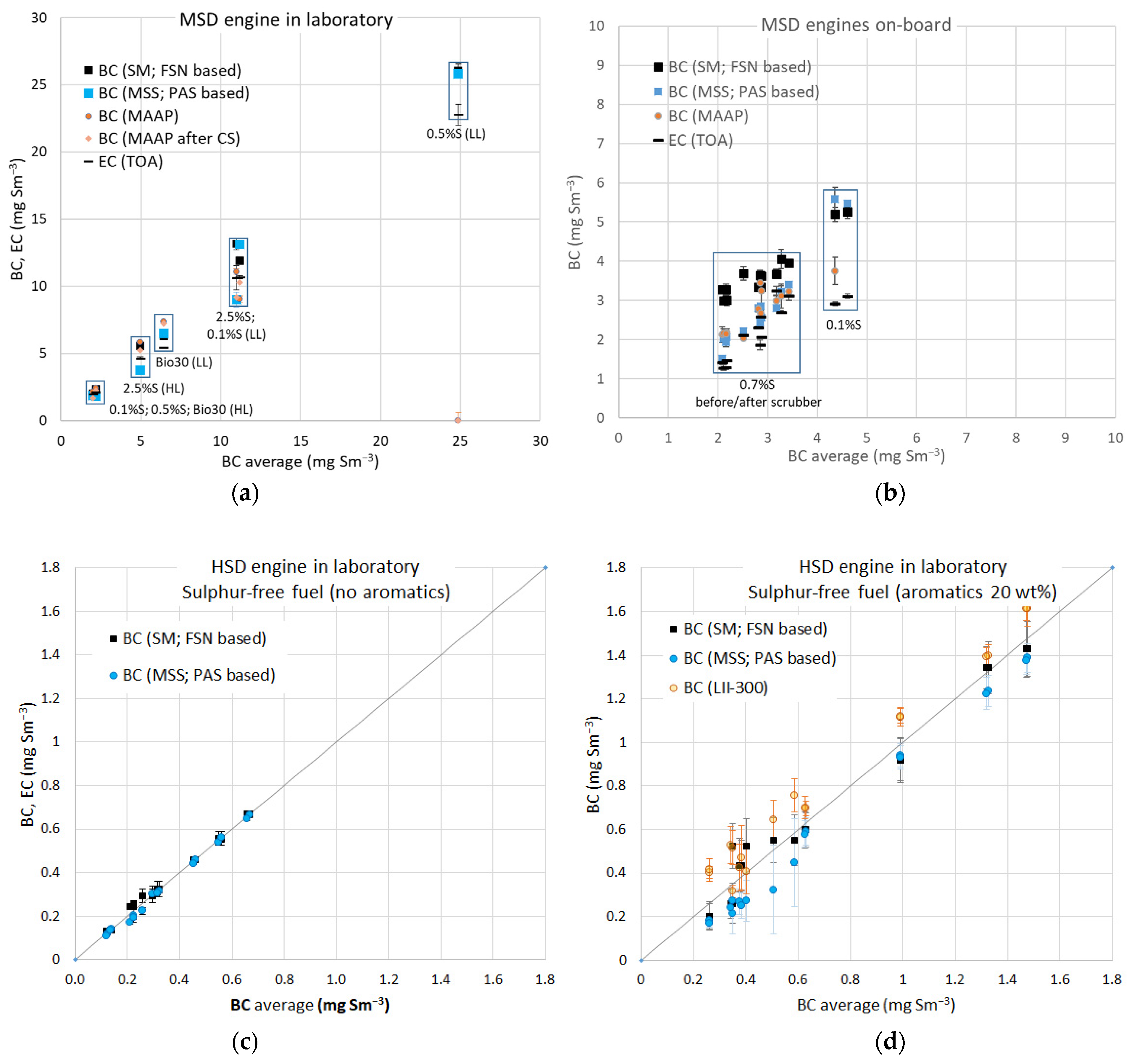
3.1.2. Overview of BC Results in Three Measurement Campaigns

Average BC results and related standard deviations of replicate tests for different fuels and engine loads in three measurement campaigns are presented in Figure 2a–d. Engine loads are not necessarily as constant in on-board measurements as in the laboratory tests; however, standard deviations were low for all three campaigns (Appendix A, Table A1).
With the laboratory MSD engine using four fuels, the BC emissions ranged up to 25 mg Sm−3 while being strongly dependent on the engine load and fuel quality, but not directly on fuel sulphur content (Figure 2a, Section S3.3 in the Supplementary Materials). The highest BC emissions were observed at low (25%) engine load for fuel with high sulphur content of 0.5%S, and at high (75%) engine load for fuel with the highest sulphur content of 2.5%S. The BC emissions were the lowest for sulphur-free, oxygen-containing Bio-FA fuel. In the on-board measurements of the modern MSD engines, BC concentrations were always low (<6 mg Sm−3), upstream and downstream of SCR and scrubber, at 40% and 75% engine loads (Figure 2b). The discrepancies between the BC results obtained with different instruments were notably high in relative terms, but within ±1.5 mg Sm−3 in absolute terms.
The lowest BC emissions (<2 mg Sm−3) were observed for the common-rail HSD engine using sulphur-free fuels (Figure 2c,d). Despite the low concentration levels, PM and BC concentrations were systemically lower for aromatic-free Ar-0 fuel than for Ar-20 fuel containing 20 wt% of aromatics. For the HSD engine, stabilised running modes of the standardised cycle were short, while for the MSD engine, durations of engine load modes were sufficient for all instruments to stabilise. Comparison of the real-time instruments, MSS(PAS) and LII 300, is straightforward even for short load modes, while the semi-continuous method used in the SM(FSN) may cause some uncertainty in time adjustment. EC(TOA) results were obtained only from the filters collected over the whole 2 × 9 mode cycle in the tests with an HSD engine.
The focus of the analysis of this study is on the behaviour of the BC-measuring instruments. However, interesting observations on the effect of fuel properties on the EC emissions were found. In campaign A, EC concentrations expectedly correlated with PAH(di+) and the asphaltene content of fuels at high engine load, while at low engine load, a correlation was found with the pour point of fuel (Figure S5 in the Supplementary Materials). Constituents related to a high pour point of fuel could induce BC emission with some engines at certain running conditions, although this first finding is indicative and may apply to specific engine types. Fuel properties have been reported to also affect the BC emissions by others [70,71,72], and lately, the effect of the aromatic content of marine fuels has also been reported (IMO PPR 8/5/1).

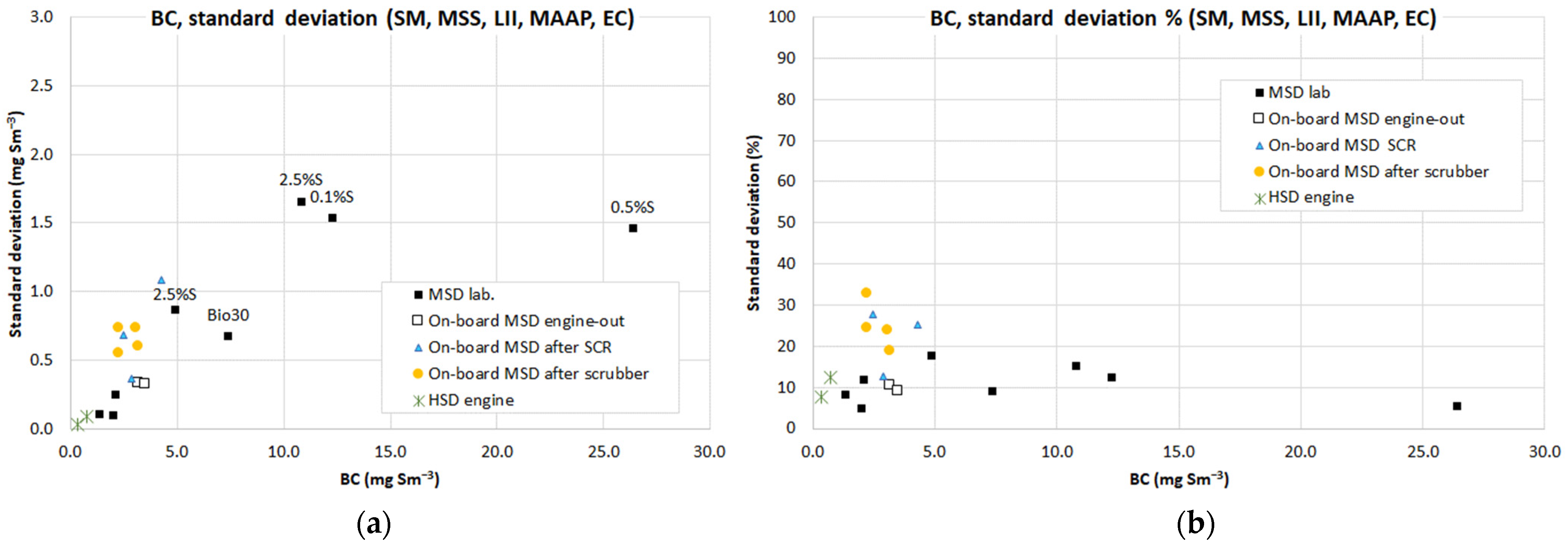
3.1.3. Statistical Analysis

The correlations between the BC results obtained with different instruments were studied by Pearson’s correlation coefficients R2 (Table 2). Differences in BC results (ΔBC) between instruments as well as their averages ( Δ ( BC ) ¯ ) and standard deviations (σ(ΔBC)) are shown in Table 2. All statistical values are calculated against the average over all instruments. The linear regression equation (BCi = a + b BC) was used to calculate the slope (b) and intercept (a) for each instrument.
The correlation was good (R2 = 0.95–0.99) between the BC results obtained by different instruments in comparison to the average over instruments. The slopes of linear regression were close to 1.0 for MSS(PAS), SM(FSN), and LII, while they were lower for MAAP and EC(TOA) (b = 0.91–0.94) and the highest for AE (b = 1.26).
A tendency for lower or higher BC results in comparison to the average over instruments is indicated by Δ ( BC ) ¯ . For the whole dataset, Δ ( BC ) ¯ was positive for SM(FSN) (0.66 ± 0.50 mg Sm−3) and for AE (0.90 ± 1.91 mg Sm−3), while it was slightly negative for MSS(PAS) and MAAP (−0.05 ± 0.74 and −0.02 ± 0.62 mg Sm−3), and particularly for EC(TOA) (−0.60 ± 0.53 mg Sm−3). For sulphur-free fuels in the HSD engine, the results from different instruments were particularly close to one another: Δ BC ¯ was slightly negative for MSS(PAS) (−0.10 ± 0.04 mg Sm−3) and slightly positive for LII (0.10 ± 0.08 mg Sm−3), while the results obtained with SM(FSN) were close to average. EC(TOA) results were also generally in line with the BC results. Lobo et al. [73] found a good correlation between the MSS and the LII 300 results, but higher concentrations for the MSS than for the LII 300, while in this work, BC concentrations were higher for LII than for the MSS. Note that the LII used here was calibrated with aviation (Gnome) engine soot.
Individual ΔBC results from SM(FSN), MSS(PAS), MAAP, and EC(TOA) were mainly within ΔBC of ±1.5 mg Sm−3 of the average results according to analysis using 90th percentile as criteria for MSD engines (Figure 3), which is a narrow difference of average when considering wide variation in the properties of the exhaust matrices studied. The largest ΔBC values were observed for aethalometers, but these were not included in the BC averages. In another study, an agreement on the BC results obtained with LII, PAS, FSN, and TOA methods was better than the one for MAAP and the aethalometer [74].
The standard deviation between results obtained with SM(FSN), MSS(PAS), LII 300, MAAP, and EC(TOA) increased in absolute terms as BC concentrations increased (Figure 4a). Aethalometers that showed the highest ΔBC results were not included in this analysis. In relative terms, the standard deviation was 5–15% for engine-out exhaust and, at a wide range of BC, concentrations were up to almost 30 mg Sm−3 (except aethalometers). After the SOx scrubber, and in some cases after SCR, deviation in relative terms was high (15–35%) due to the low BC concentration level (<5 mg Sm−3), although deviation in absolute terms was only <0.8 mg Sm−3. For engine-out exhaust at the same BC concentration level, deviation was even lower in absolute terms (<0.4 mg Sm−3). For the HSD engine, the deviation of the BC results was higher when Ar-20 fuel was used than when aromatic-free Ar-0 fuel was used, and the aromatic content of fuel influenced the BC results and comparability between instruments.
More details of the BC results and inter-correlations with the SM(FSN) and MSS(PAS) techniques, instruments designed for ambient measurements (MAAP, aethalometers), and EC(TOA) from ISO 8178 and in-stack sampling are available in the Supplementary Materials (e.g., Figure S7). Note also that MAAP’s narrow measurement range was exceeded at the highest BC concentrations, even at DRs above 600.

3.2. The Effect of PM Composition on Instrument Behaviour

3.2.1. Sulphates, Metals, Organic Carbon, and Equivalent Light Absorbing Carbon of PM

Considering the different instruments used, and various dilution conditions and exhaust matrices, correlations in the BC results were surprisingly good (see previous section). However, deviation in the BC results was sufficiently large to evaluate the effect of exhaust properties on the instrument behaviour. Of the characterised exhaust properties, especially interesting were sulphates, metals, and organic fraction of PM (Appendix A, Figure A1).
Sulphates were present in PM when using residual fuels and were found to increase with increasing fuel sulphur content [15,75], although the relationship between fuel sulphur and exhaust SO42 concentrations is not straightforward due to promotion of SO3 precursor at high combustion temperatures. The share of SO42 in PM was higher at 75% engine load than at 25% engine load (13–35% versus 2–7% of PM) in campaign A, with the MSD engine using four fuels (0–2.5%S). In the on-board campaign B, exhaust PM contained substantial amounts of SO42 both before and after the scrubber when using 0.6%S fuel. In combination with varying organic fractions of PM, the exhaust composition downstream of the SCR and SOx scrubber was unique.
Metal oxides and sulphates (ash) are typically found in engine exhaust PM originating from fuel (e.g., with asphaltenes), lubricating oil, or engine wear. In campaign A, exhaust PM contained substantial amounts of metals when using residual 2.5%S and 0.5%S fuels (V 5.9–8 mg Sm−3, Ni 1.4–1.7 mg Sm−3), and to a lesser extent in campaign B on-board (V 0.28–0.43 mg Sm−3, Ni 0.20–0.28 mg Sm−3, Fe 0.23–0.35 mg Sm−3, and Na 0.23–0.46 mg Sm−3). Ca was also present in exhaust PM, likely originating from Ca observed in fuels and lubricating oil. Exhaust PM contained substantial amounts of water and oxygen attached to sulphuric acid and metal salts. For the HSD engine, exhaust PM did not contain significant amounts of SO42 or metal salts, albeit some Ca, Na, and Ni were present in PM (<0.04 mg Sm−3). Ni, Na, Cr, and Cu indicate engine wear, Ca lubricating oil of MSD engines, and Zn lubricating oil of HSD engines.
Organic carbon is typically a substantial contributor to exhaust PM mass emissions from marine diesel engines. The OC fraction of PM is not uniform, since coloured (BrC type) and colourless compounds with varying tendencies to absorb light may be present. Dilution with moderate DR promotes OC condensation on the filter due to phase partitioning of semi-volatile organic compounds, and cooling of diluted exhaust further shifts OC from gas to particle phase [76]. The share of OC in the PM was the highest (56–77%, diluted) for the 0.5%S fuel in campaign A, while in campaign B, the share of OC in PM reduced over the SCR. For the HSD engine, the PM emission practically only contained EC (18–21%) and OC. Typically, diesel engines using sulphur-free fuels contain only a low share of non-BC material [9]. The absorption Ångström exponent (AAE) describes the spectral dependence of light absorption by aerosols. Helin et al. [29] observed high AAE470/950 values (0.9–1.3) for high-sulphur marine fuels, potentially linked to high PAH and metal salt content in PM. All PM samples contained PAHs. The sum of the six priority PAHs was 3–17 µg Sm−3 with campaign A, 1.7–6.5 µg/Sm−3 in campaign B, and only <0.7 µg/Sm−3 in campaign C. The removal of volatiles from exhaust using a thermodenuder or a catalytic stripper is reportedly less significant than the removal of non-volatile light-absorbing organics or metal salts for distinguishing BC from other light-absorbing compounds [29,51,59]. For further analysis, the concentration of light-absorbing compounds was calculated as a product of the AAE470/950 ratio and BC concentrations (AAExBC).

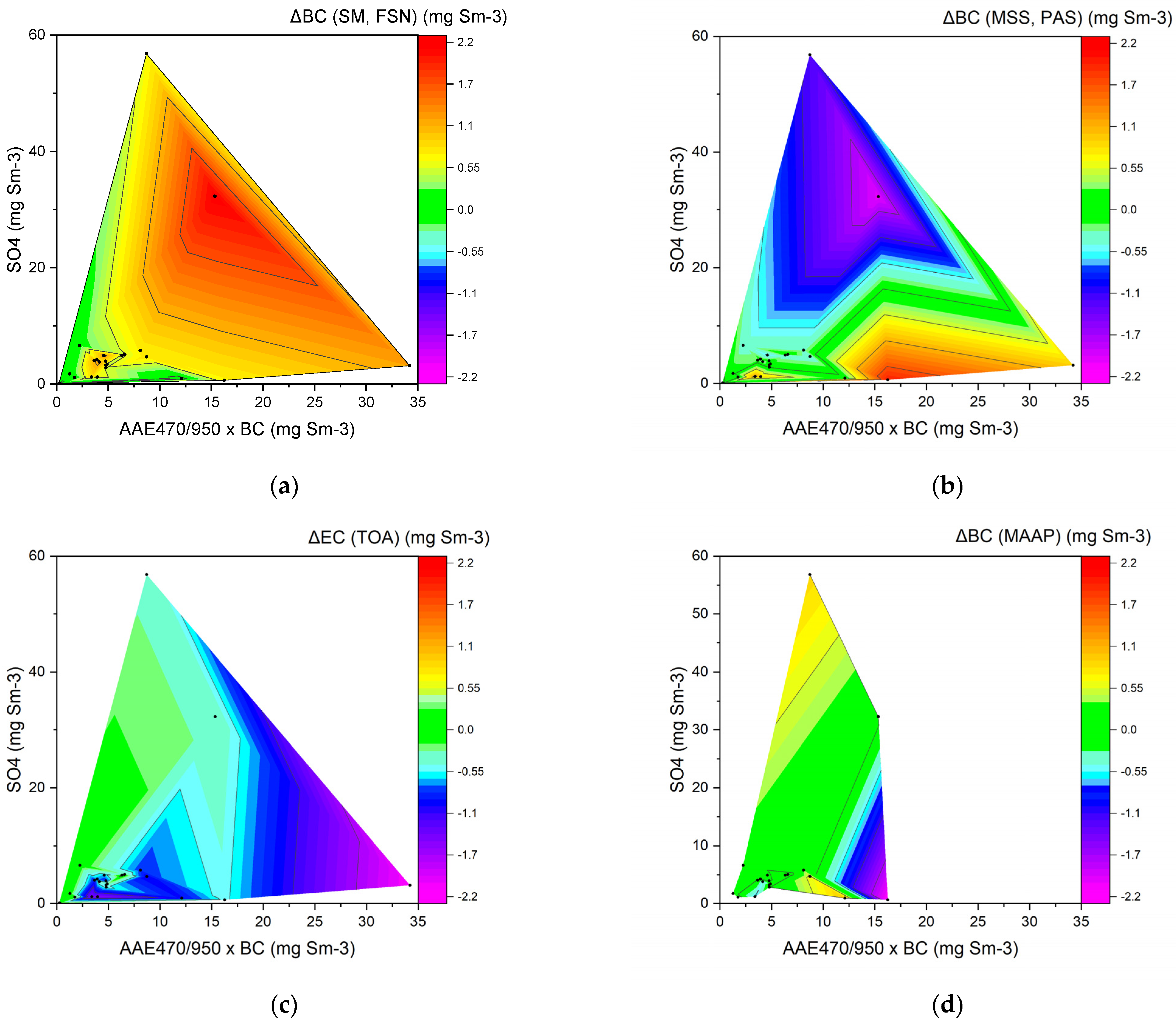
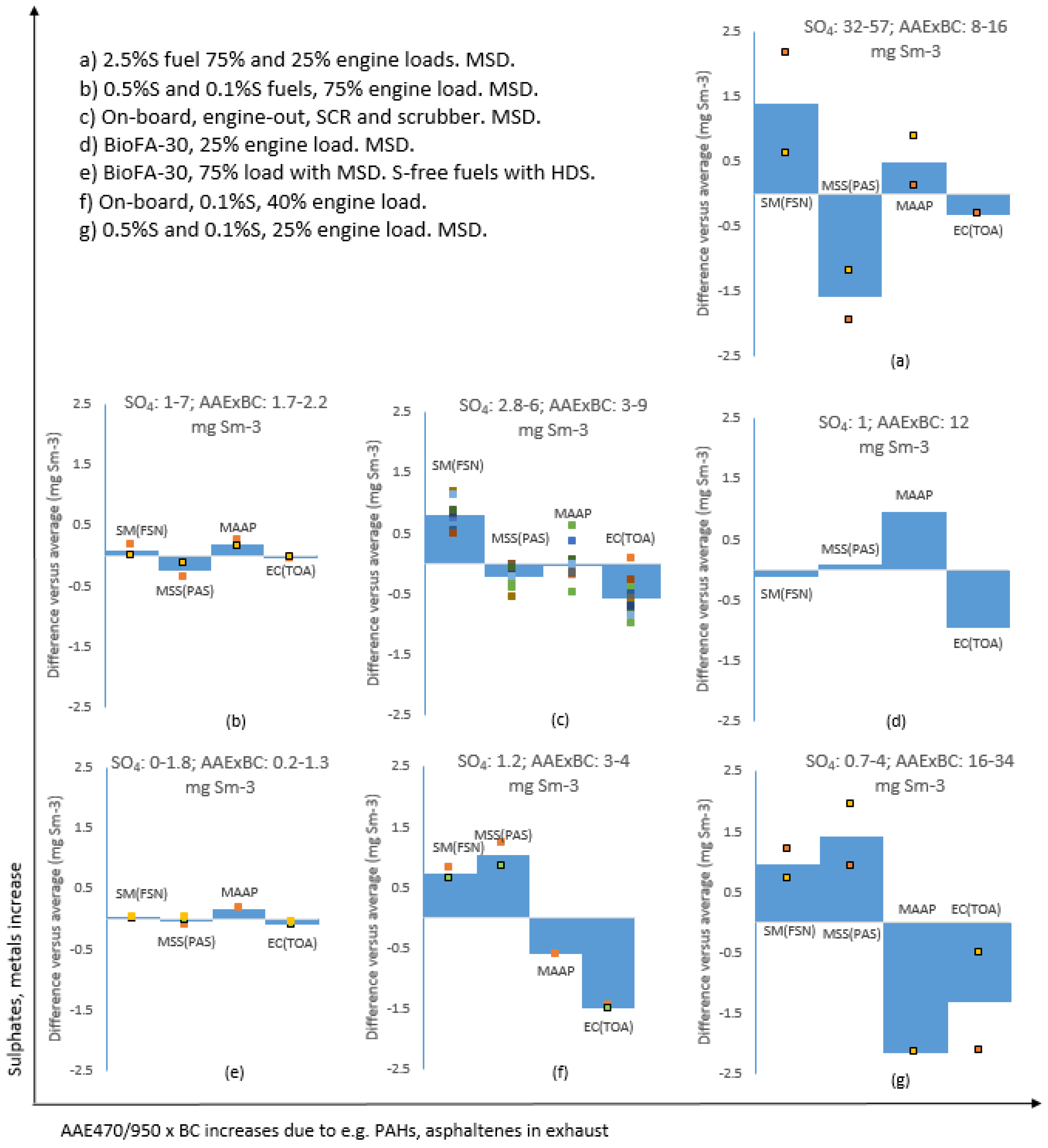
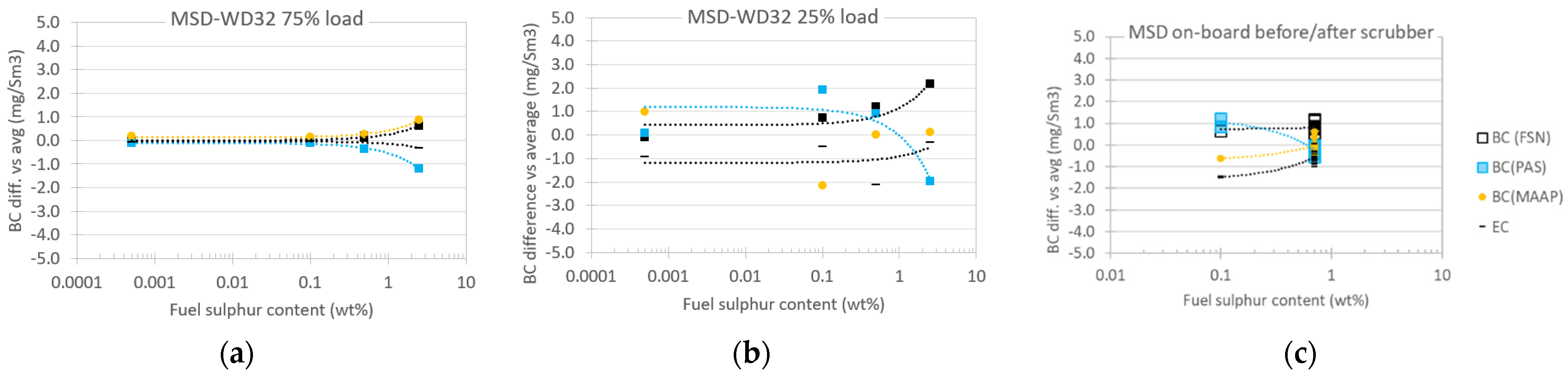
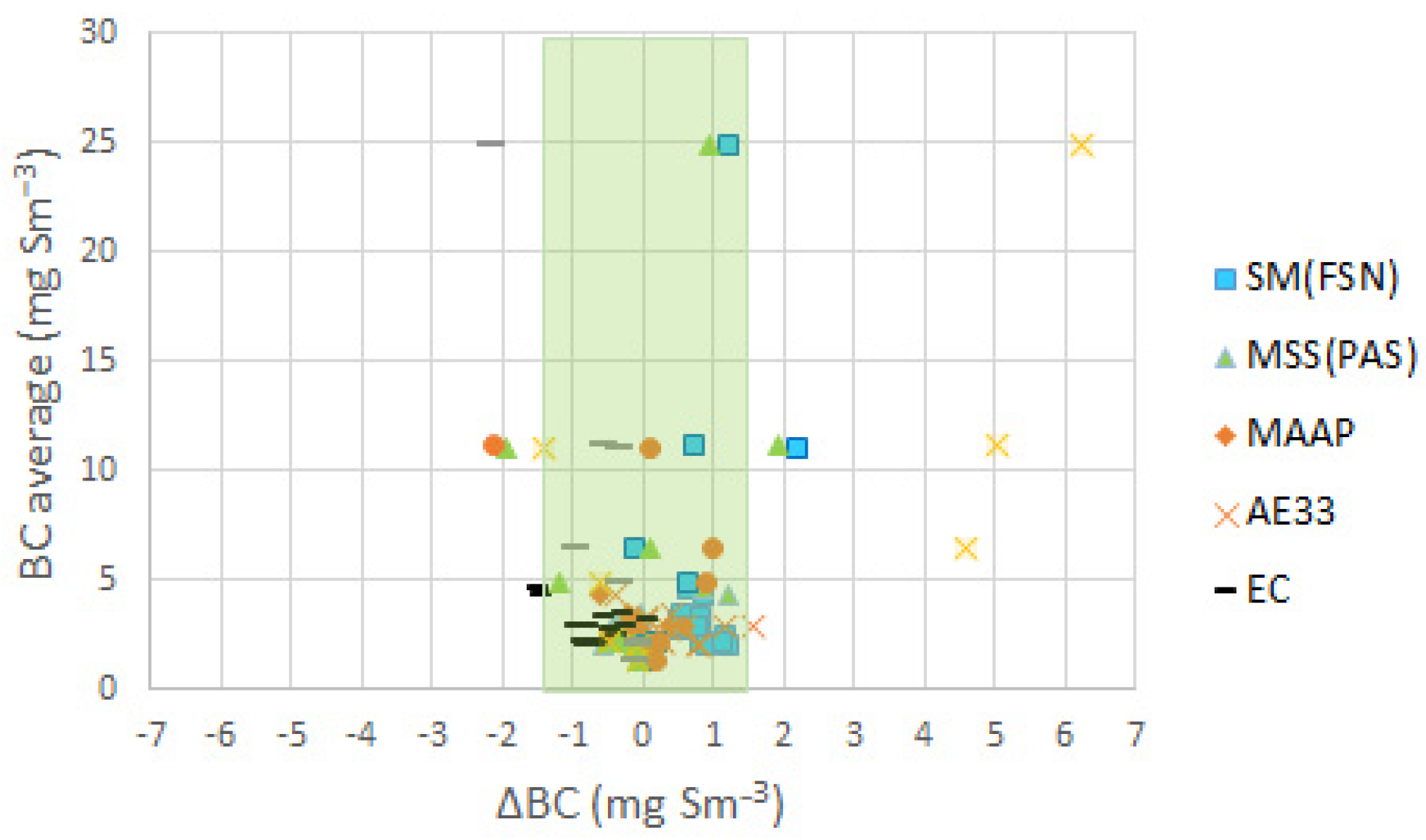
3.2.2. Analysis of the Effect of Exhaust Properties in the BC Results Obtained with Different Instruments

Regression analyses of the ΔBC results and exhaust properties were carried out, and squared Pearson’s correlation coefficients are presented in Appendix A, Table A2. Several exhaust properties, such as SO42, AAE470/950, AAExBC, metals, CO, and NOx concentrations seemed to correlate with instruments in individual measurement campaigns, but not over all campaigns. Dependencies were not found between BC concentrations and diluted OC:EC ratios or the AAE470/950 values, while AAE470/950 correlated with the raw exhaust (in-stack) OC:EC ratios (Figure S5 in the Supplementary Materials).
In continuation, the effects of the SO4 and AAExBC on ΔBC between instruments were studied (Figure 5), and some systematic behaviours of instruments were observed. SM(FSN) showed positive ΔBC at high SO4 and AAExBC concentrations, and elsewhere ΔBC was close to average (neutral, green region). For MSS(PAS), ΔBC was generally negative, and at high SO4 concentration even more negative than for EC(TOA), while positive ΔBC was found only at a low SO4 level. EC(TOA) showed the lowest BC emissions of instruments (negative ΔBC) or similar BC level as the other instruments, with the exception of lower ΔBC for MSS(PAS) at high SO4 concentrations. With MAAP, ΔBC was mainly positive or neutral; however, the highest BC concentrations exceeded the measurement range of MAAP even at DR of 600. Overall, BC concentrations measured with the MSS(PAS) and EC(TOA) were in most cases lower than BC concentrations measured with the SM(FSN) and MAAP.
A more detailed look at the combined effect of SO4 and AAExBC on measured BC is presented in Figure 6, with separate subplots for different measurement points. For exhaust containing a low or moderate level of AAExBC and SO4, different instruments resulted in BC results close to each other (low ΔBC, Figure 6b,e), particularly for sulphur-free fuels (<0.001 wt%). Hence, the lowest ΔBC between the instruments was observed at the lowest AAExBC and SO4 concentrations. The following observations can be made regarding instrument behaviour:
  • SM(FSN) showed positive or neutral ΔBC in all cases.
  • EC(TOA) showed negative or neutral ΔBC in all cases.
  • MSS(PAS) showed negative or neutral ΔBC in most cases. Exceptions are positive ΔBC for 0.1%S and 0.5%S fuels at 25% load (campaign A) and for 0.1%S fuel in on-board tests (campaign B) (Figure 6f,g). In these cases, AAExBC was elevated, while SO42 level was low. Notable also is the very low BC level at the highest SO42 level, even lower than that for EC(TOA) (Figure 6a).
  • MAAP showed higher BC concentrations than the MSS(PAS) and EC(TOA) in most cases (7abce). Exceptions with negative ΔBC were observed in the same cases as exceptions for MSS(PAS) in Figure 6f,g.
SM(FSN) and EC(TOA) behaved as expected and systematically regardless of the exhaust’s composition. Noted is that EC(TOA) was analysed from extracted samples to reduce bias and to improve the reliability of the analysis, whereas OC(TOA) was analysed from untreated samples [15].
The positive ΔBC for MSS(PAS) and negative ΔBC for MAAP (Figure 6f,g) were the opposite of the general trends observed for these instruments. These results were obtained under two conditions: a) with 0.1%S and 0.5%S fuels where AAExBC concentrations were high (16–34 mg Sm−3) and b) downstream of the SCR with 0.1%S fuel where AAExBC concentration was medium (3–4 mg Sm−3). In both cases, SO4 concentrations were low (1.2 and 4 mg Sm−3), and so were fuel-related metal salt concentrations. None of the exhaust properties alone directly explained this phenomenon; however, a high ratio of AAExBC:SO4 may potentially affect instrumental behaviour regarding the obtained BC results. The BioFA ratio of AAExBC:SO4 was high (Figure 6d), but the ΔBC values remained small, which was due to very low BC emission. In addition, unexpected behaviour of MSS(PAS) and MAAP was observed downstream of SCR at slightly higher BC levels (Figure 6f), while it was not at slightly lower BC levels (Figure 6c). Hence, morphology or particle sizes could affect BC measurements through changes in extinction and scattering of mass coefficients (Figure S7 in the Supplementary Materials; [77]). The mass extinction coefficient of BC is nearly constant for ultrafine particles (<100 nm), but changes in larger particle sizes, which are present, for example, after scrubber [78] and in aging of exhaust with grown particles via gas-to-particle processes condensing on primary BC particles [29]. Detailed characterisation of particle sizes and morphology would warrant attention in future studies. Exhaust aerosol with a high content of AAExBC and moderate content of SO4 and metals may become more typical than before with the introduction of the 0.5%S limit globally in 2020.
The BC level measured with MSS(PAS) was lower than with EC(TOA) at very high SO42 concentrations (Figure 6a, Appendix A, Figure A2), although results obtained with these instruments are typically close to each other due to calibration of the MSS(PAS) with EC(TOA). The presence of interfering compounds in residual fuels may affect EC(TOA) results, and this may not be fully taken into account in the calibration of MSS(PAS) (or other instruments) with EC(TOA).
In the tests with the SCR or SOx scrubber (Figure 6c), combination of the low or moderate AAExBC concentration and high SO42 concentration presents an exceptional composition of exhaust when compared to traditional diesel exhaust. However, ΔBC between instruments followed the general patterns in other cases than in the measurements from downstream of the scrubber using 0.1%S fuel, which was discussed in relation to Figure 6f. Notably, overall differences in BC concentrations obtained with different instruments were low.

3.3. Other Factors Affecting Comparability of the BC Results

3.3.1. Correction Factors Used for BC Measurement Instruments

Generally, correction factors are used in the calculation of BC results obtained by different instruments. Identifying potential artefacts has led to corrections for MAAP [18] and aethalometers [30,67]. Different BC sources may warrant specific correction factors and algorithms [79], including exhaust from marine diesel engines using residual fuels.
BC-dependent variation of MACBC is known for optical BC measuring principles, for example, MACBC for fresh BC is reportedly on average 7.5 ± 1.2 m2 g−1 at 550 nm, but the range from 4.3 to 15 m2 g−1, and values even up to 50 m2 g−1 have been reported (references in [9]). For the SM(FSN) instruments based on light absorption, the MACBC calculated in this study was 6–8 m2 g−1 at 550–570 nm at BC concentrations below 20 mg Sm−3, and it gradually decreased at higher BC concentrations (Figure 1). A non-linear relationship between MACBC and BC concentrations may be due to different BC and non-BC species, the morphology of the particles, the age of the aerosol, and the size of the particles, as well as the loading of the filter and the measured wavelength. Generally, source and BC-concentration-dependent correction factors used for different BC measuring instruments may explain some of the differences observed in studies, indicating that correction factors may not sufficiently take account of all types of exhaust.

3.3.2. Measurement Range of Instrument, Pre-Treatment, and Necessity of Dilution

Detection limits and measurement ranges of BC measurement instruments need to be sufficient for the BC concentrations measured. With the MSS(PAS) and LII 300 instruments used here, LoD was 0.005 and 0.002 mg Sm−3, and for the SM(FSN) instrument, LoD was 0.02 mg Sm−3.
The capability to measure raw or diluted exhaust varies between instruments. The SM(FSN) was the only instrument in this study designed for measuring raw exhaust gas. The MSS(PAS) and LII 300 need at least some dilution to measure ship exhaust containing sulphates and metal salts. The ability to measure high concentrations is a benefit when determining BC in raw exhaust from diesel engines, as using dilution air always leads to more uncertainty in results, especially if very high dilution rates are required. DR is a multiplier in the calculation of the BC results, and any uncertainty is directly reflected in the BC results. Measurement ranges for instruments designed for ambient air are narrow, and high DRs are typically needed for measuring BC from diesel engines.
For all measurements, and particularly when measuring the raw exhaust, lowering the sample air temperature is necessary to protect the instrument. Condensation is specifically a threat when sampling raw exhaust. When using high-sulphur fuels, clogging of diluters (heated or non-heated) and corrosion-related problems are also potential threats. The durability of the SM(FSN) is proven for marine engine exhaust.
Removing volatiles could alleviate bias in some BC measurement techniques (Figure S6 in the Supplementary Materials); however, it would do so at the cost of increased complexity of the test setup, potentially inducing new problems and losses of BC as discussed before [51]. The methods studied here are mostly used in laboratory, and on-board measurements bring more challenges if dilution or pre-treatment is applied. In aircraft certification, sampling with LII applies a DR of 8, and a catalytic stripper is used for high-sulphur fuels (3000 ppm).

3.3.3. Sampling

Sampling of raw exhaust is one of the determining steps in engine exhaust measurements towards reliable results regardless of instrument, and a starting point for achieving comparable results with different instruments. General recommendations on sampling and conditioning of raw exhaust from engines are given by standards (e.g., ISO 8178), and good practices are applied in laboratories. Instrument manufacturers have also presented guidelines (e.g., [42,65]). Some practical issues from the mentioned sources are listed as follows:
  • A sampling probe (stainless steel) should be located in the centre of an exhaust duct, in a straight section to avoid pressure fluctuations. A 45° bevelled probe should have an opening facing the flow of the exhaust stream. This setting is less significant for particles <200 nm than for those >400 nm, which escape sampling if the cap is used.
  • The transfer and sampling lines should be as straight and as short as possible, preferably maximum 3 m. For high-sulphur fuels, recommended SM (AVL) sampling lines are from 4–8 m and are in an ascending layout from sampling that point to the device.
  • Sampling lines should have a smooth inner surface to lower the contamination effect. Bends and edges should be avoided to minimise particulate (turbulent) deposition. Fast dilution reduces thermophoretic losses, for which correction factors can be calculated (ISO 8178-1 Annex, 2017), if not applied automatically by instruments.
  • Heated sampling lines are needed to avoid condensation, which occurs depending on the dew point of the water and sulphuric acid, and heat transfer through the line walls. Diluters also need heating. The sampling probe may need heating when measuring exhaust after a scrubber to avoid droplets in instruments (applied in the on-board campaign of this study).
  • The sampling line purging with compressed air lessens condensation and contamination during measurements (some instruments have this option).

3.3.4. Thermophoretic Losses

Thermophoretic losses can affect BC particles when sampling engine exhaust. This is not necessarily an issue in the ambient air measurements where the temperature gradient is low. In exhaust measurements, BC may deposit on the walls of transfer line between raw exhaust sampling point and diluters or instruments due to temperature differences between the walls and the raw exhaust. Thermophoretic losses are greater for BC particles than, for example, inertial losses and turbulent diffusion [80].
In the instruments used in this study, thermophoretic loss was automatically corrected in the BC results only by the SM(FSN) instrument. Thermophoretic loss was manually corrected in the results for MSS(PAS) and LII 300 in this study (factors for MSD engines 1.11–1.17, SOx scrubber 1.0, HSD engine 1.0–1.12, see Section 2.2). Thermophoretic loss correction was not applied for EC(TOA), MAAP, or aethalometers. The BC results without corrections of thermophoretic losses may be underestimated to some extent. Jiang et al. [81] also reported factors of 1.22–1.29 times between BC emissions from the SM(FSN) (with correction), and LII and PAS (without correction) due to differences in applying corrections of a thermophoretic loss.
We note that correction of thermophoretic loss is not standardised or systematically applied, and hence it is a possible source of ΔBC between different instruments.

3.3.5. Data Processing

Data processing varies for different BC measurement instruments. Output from the SM(FSN) is on screen or saved on a computer in an easily accessible format. The MSS(PAS) saves the results at high resolution: one second intervals were used in this study, but 10 Hz intervals would be an option. For the MSS(PAS), the data format is easily readable with common programs (e.g., Excel). For the LII 300, data resolution is adjustable, and for these measurements, recording in 5Hz intervals was recommended and used, which led to large file sizes. Data files from LII were not readable with common programs and data processing required special software. LII 300 data processing also required a user familiar with instrument settings, since the results are influenced by the choices made. Otherwise, all three instruments, SM(FSN), MSS(PAS), and LII 300, were straightforward to use. Additionally, SM(FSN) and MSS(PAS) instruments used converted concentrations in the defined temperature and pressure, while for LII this conversion is optional and would deserve to be reported in the data output file.

3.3.6. Calibration and Traceability

Calibration procedures for instruments are presented in the standards and manufacturer guidelines (Section S1 of the Supplementary Materials).
Traceability is optimally available for a measured property. However, the BC measurements today are not traceable, since there are no commonly agreed upon “reference instruments” or standard reference materials (SRM) of BC to be used in calibrations [19]. Additionally, all of the BC-measuring instruments use their own (calibration) factors to calculate the result from the measured quantity, and these factors change when the properties of the measured aerosol change. One of the methods for atmospheric aerosol absorption calibration considered is the extinction minus scattering (EMS) technique; however, even this technique may be sensitive to interference with high NOx concentrations present in the engine exhaust. Reference methods (materials, aerosol generators, or instruments) or defined parameters and conditions can be agreed upon by standardisation organisations. It is noteworthy that PM emissions are regulated in the road sector, although PM is at least as complex an emission species as BC, and measurement methods are also not traceable.
Defined requirements for instruments and their validation protocols are needed for the expected regulatory BC measurements drawn from marine engines. Typically, instrument manufacturers define instrument-specific calibrations and maintenance (e.g., flows, sample cell cleaning) and other factors that are a part of quality assurance in the laboratory conducting the measurements, in addition to regulations, standards, and good practices of laboratories. We note that the results here apply to the instruments used, and standards are needed to extend them to other instruments using the same measurement principles. For standardised measurements, defined requirements for instruments and parameters are set, as well as defined produces for sampling, measurement, and calibrations. Out of the measurement techniques studied here, SM(FSN), MSS(PAS), LII 300, and EC(TOA) are standardised for measuring exhaust from internal combustion engines, but only the SM(FSN) standard covers marine engines. MAAP and aethalometers are designed for ambient air measurements and consequently demand dilution and sample treatment when measuring high BC concentrations of diesel engine exhaust, although they are proven to work in, for example, plume measurements where BC concentrations are low. A summary of exhaust properties and instrument characteristics is given in Table A3.

4. Conclusions

BC concentrations were measured from diesel engines using the IMO’s candidate methods, FSN, PAS, and LII, and instruments commonly used in ambient studies (MAAP, aethalometers, TOA). Extensive exhaust matrices were obtained by using various engines, emission control technologies, and fuels. With the MSD engine in laboratory, fuels with 0.1%, 0.5%, and 2.5% sulphur content and biofuel were used. On-board a modern ship, emissions from two MSD engines with 0.6% and 0.1% sulphur content fuels were measured upstream and downstream of SCR and SOx scrubbers. With the HSD engine in laboratory, sulphur-free fuels with two levels of aromatics (0% and 20%) were studied. The PM composition varied from high to low content of sulphates, metals (e.g., V, Fe, Ca, and Ni), and low-volatility organic compounds offering extensive exhaust matrices for research on the suitability of different methods for measuring BC emissions from marine engines.
Correlation between the BC results obtained with the smoke meters (AVL 415S, AVL 415SE), AVL MSS (PAS), LII (Artium-300), MAAP 5012, and aethalometers (Magee AE-33, AE-42) was relatively good, and the EC results also compared rather well with the BC results (R2 0.95–0.99). LII 300 and SM(FSN) showed slightly higher BC concentrations than MSS(PAS) in the HSD engine campaign. The standard deviation between instruments (excluding aethalometers) was in the range of 5–15% for engine-out exhaust at BC concentrations <30 mg Sm−3. After SOx scrubber, and in some cases after SCR, deviation was higher in relative terms (15–35%), while in absolute terms it was only <0.8 mg Sm−3.
Differences between the BC results obtained by instruments in comparison to average over instruments is designated by Δ(BC). The observed 90th percentile of ΔBC was ±1.5 mg Sm−3, which is a narrow range when considering the wide marine exhaust matrices studied. Typically, BC concentrations measured with SM(FSN) and MAAP were higher than those measured with MSS(PAS) or EC(TOA). The ΔBC was consistently positive for SM(FSN) (+0.66 ± 0.50 mg Sm−3) and negative for EC(TOA) (−0.60 ± 0.53 mg Sm−3), while for MSS(PAS) and MAAP the direction of Δ ( BC ) (−0.05 ± 0.74 mg Sm−3 and −0.02 ± 0.62 mg Sm−3) depended on the aerosol properties, ratio of AAExBC:SO4, or on particle sizes and morphology, which is a new finding.
Regression analysis of the results revealed correlations between ΔBC and exhaust properties in individual measurement campaigns, but not over the whole dataset, indicating that combined effects of aerosol properties could be significant. Indeed, interaction of ΔBC and concentrations of light-absorbing compounds (AAE470/950xBC) and SO42 was found. The negative ΔBC for MSS(PAS) was expected following the EC(TOA) used in calibration MSS(PAS). Unexpectedly, ΔBC was positive for MSS(PAS) in some conditions. Analysis showed that this was potentially explained by combination of high AAExBC (16–34 or 3–4 mg Sm−3) and low SO4 concentrations (1.2 and 4 mg Sm−3; also low metal salt concentrations). The direction of ΔBC for MAAP was also different for these than the other exhaust compositions. The magnitude of ΔBC was the smallest at low AAExBC and SO4 concentrations of exhaust.
Besides exhaust properties, instrument correction factors and representativeness of sampling affect the capability of instruments to achieve comparable BC results. For example, correction of thermophoretic loss of BC in the transfer line was automatic only for SM(FSN), while thermophoretic loss needs to be corrected by users for other instruments. For the sampling of hot and humid diesel engine exhaust, the SM(FSN), MSS(PAS), and LII 300 instruments were practical, while special dilution to obtain a high dilution ratio was needed for MAAP and aethalometers. Sampling for EC(TOA) used a standardised system. Data output from the SM(FSN) and MSS(PAS) instruments was easily accessible without special software or an experienced user, and data was in the specified temperature and pressure, which was not the case for all instruments. Many other issues should be taken into consideration also, for example, calibrations and durability. The SM(FSN) instrument is standardised covering marine engines using residual fuels, while the MSS(PAS) is a standard method in road and aviation sectors, and LII 300 is standard in the aviation sector.
The results showed that the BC measurement instruments studied distinguished BC concentrations from marine engine exhaust even when the exhaust composition varied substantially. Differences in BC emissions obtained with studied instruments were affected at least to some extent by exhaust constituents and further improvements, for example, by developing methods for calibration and determining correction factors one could improve measurements of challenging exhaust from ships. Differences in correction of thermophoretic losses should be considered. Novel findings include an observation that individual exhaust properties may not explain differences between instruments, while the (AAExBC):SO4 ratio seemed significant. New combinations of exhaust properties appearing with high-sulphur fuels will remain in the SOx scrubber-equipped ships, while fuels below 0.5% sulphur still contain residual components, and emission control (SCR, scrubbers) is increasingly used. In summary, BC results obtained with instruments selected by the IMO correlated well even with challenging exhaust compositions, and differences between instruments were relatively low. Further improvements are possible by appropriate standardisation of procedures for sampling, correction factors, and calibrations.

Supplementary Materials

The following are available online at https://www.mdpi.com/article/10.3390/atmos13010031/s1, Sections S1.1–S1.5: BC measurement instruments. Section S2: Engines, test set-up and fuels in three test campaigns. Section S3: Support to the results and discussion. Section S4: Particle sizes affect extinction and scattering mass coefficients. Section S5: Numerical results. Figure S1: Relationship between BC and FSN. Figure S2: LII scheme. Figure S3: Overview of the instrumentation in the BC measurements in laboratory campaign A. Figure S4: Correlations between OC:EC and UV370:BC880 with AAE values, laboratory MSD campaign. Figure S5: Correlations between fuel properties and EC concentrations in exhaust for the LAB-MSD engine with 25 and 75% loads. The fuel aromatic content and pour point shown in left axis and fuel ash content (wt%) in right axis. Figure S6: Instruments in the same dilution line (DR 600–1800, aged particles) and correlation between two SM instruments, laboratory measurements with MSD engine. With courtesy of CIMAC [51]. Figure S7: Particle size distribution affect the extinction and scattering mass coefficients. Table S1: Calculation of the results by aethalometer MAGEE 33 (MAGEE manual (MAGEE, 2015). Table S2: Specifications of the MSD engine in laboratory. Table S3: Properties of the test fuels in MSD engine campaigns. Table S4: Specifications of the AGCO diesel engine. Table S5: MSD engine in laboratory, campaign A. Gaseous emissions, PM and its composition, BC (FSN-based), metals and PAHs. Table S6: On-board MSD engine in laboratory, campaign B. Gaseous emissions, PM and its composition, BC (FSN-based), metals and PAHs.

Author Contributions

Conceptualisation, funding acquisition, and supervision, P.A.-S., H.T., T.R. (campaigns A–C) and P.J. (campaign C); methodology design, experiments, data curation, investigation, and validation, P.A.-S., H.T., T.R., T.M., K.T., P.K. (Päivi Koponen), N.K., M.A., P.K. (Panu Karjalainen) (campaigns A–C), H.V. (campaigns A, B), K.L. (campaign B), A.J., S.S., L.S., L.M.F.B., I.K.O. and D.D. (campaign C). P.A.-S. wrote the original draft of the manuscript and designed the visualisation. All co-authors participated in the writing, review, and editing of the manuscript. All authors have read and agreed to the published version of the manuscript.

Funding

This research was funded by Business Finland (SEA-EFFECTS BC No 40356/14 and BC footprint No 1441/31/2019), Traficom (198717/02.03.00/2020), the European Union’s Horizon 2020 programme (H2020 TUBE No 814978), Academy of Finland Flagship funding (grant nos. 337552, 337551), and from industrial partners.

Institutional Review Board Statement

Not applicable.

Informed Consent Statement

Not applicable.

Data Availability Statement

Data is available as Supplementary Materials.

Acknowledgments

The authors wish to thank Jorma Kämäräinen and Anita Mäkinen from Traficom for their support and consultation related to the BC emissions from marine engines. Thanks are given for assistance in measurement planning to Heikki Korpi (Wärtsilä). The authors also wish to thank Liisa Pirjola (Metropolia) for lending an Aethalometer in campaign A. Authors deeply thank personnel for their invaluable contributions to the project’s measurements: Pekka Piimäkorpi (campaigns A–C), Sami Nyyssönen, Jarmo Kuusisto, Jarno Martikainen, Matti Niinistö (campaign A), Mikko Karppanen (campaign C), at VTT, Matthew Bloss at FMI, Pauli Simonen, Teemu Lepistö at TAU.

Conflicts of Interest

The authors declare no conflict of interest.

Appendix A

Table A1. PM, BC, and EC concentrations and ratios of OC/EC and AAE470/950 at low and high loads in campaigns A and B and over cycle in campaign C.
LoD/Range
(mg Sm−3)
DRSample Concentrations
(mg Sm−3)
Raw Exhaust Concentrations
(mg Sm−3)
Raw Exhaust Concentrations
(mg Sm−3)
A.MSD laboratory Min.Aver.Max.75% engine load25% engine load
Bio300.1%S0.5%S2.5%SBio300.1%S0.5%S2.5%S
BC, FSN principle0.02/32,00011.48.725.91.42.02.45.86.412.125.913.6
BC, PAS principle0.005/100070.21.13.71.31.91.83.86.513.125.89.0
BC, MAAP 0.0001/0.06 *~200/>6000.0030.0110.061.52.22.45.87.49.1*11.1
BC, AE330.00003/0.1~200/>6000.0020.0190.161.31.91.74.411.016.231.19.6
EC0.2/1–15 **80.20.92.81.32.02.14.65.510.722.810.7
OC:EC diluted 8 8.37.211.43.96.74.33.14.9
OC:EC raw exh. 1 0.700.510.621.310.720.400.341.28
AAE470/950 10.91.321.111.11.6
PM 82.29.219.117.920.543.7152.952.563.5102.9134.2
Average BC, EC 1.32.02.14.97.412.326.410.8
BC,EC, st.dev. per instrument 6.7%3.1%3.7%8.5%1.8%4.3%2.0%6.1%
BC,EC st.dev. over instruments 8.2%4.9%11.9%17.7%9.2%12.5%5.5%15.3%
B.MSD, on-board MSD1, pre-scrub.after scrubberMSD2, pre-scrub., after SCRafter scrubber and SCR
Engine load 75%40%75%40%75%40%40%75%40%
Fuel sulphur content 0.6%S0.6%S0.6%S0.6%S0.6%S0.6%S0.1%S0.6%S0.6%S
BC, FSN principle***13.33.85.23.74.03.63.63.73.35.23.33.0
BC, PAS principle***70.20.40.82.83.42.42.62.22.85.61.52.1
BC, MAAP ***125–2110.010.020.033.03.23.53.22.02.83.82.12.2
BC, AE33***125–2110.010.020.043.23.84.04.52.33.24.02.92.5
EC***101.42.43.23.23.11.92.12.12.32.91.41.5
OC:EC diluted 8.28.07.37.95.22.71.65.13.1
AAE470/950 2.01.72.21.81.81.50.91.61.5
PM 10 52.247.229.938.127.520.514.221.716.9
Average BC, EC 3.23.53.13.22.52.94.32.22.2
BC,EC, st.dev. per instrument 2.8%2.6%3.7%3.9%2.3%2.3%4.9%4.4%4.1%
BC,EC st.dev. over instruments 10.4%9.2%23.8%18.9%27.8%12.8%25.3%32.8%24.5%
C.HSD laboraory Ar-0Ar-0Ar-20Ar-20Aver. Ar-0Aver. Ar-20
Low DRHigh DR High DR
BC, FSN principle***10.120.551.20.37-0.75-0.370.75
BC, PAS principle***1–400-00.121.250.350.390.620.730.370.67
BC, LII principle0.002270–400000.01---0.88 0.88
EC***8---0.31-0.64-0.310.64
OC:EC diluted 2.691.54
AAE470/950
PM ----1.00-1.83-1.01.8
Average BC, EC 0.350.73
BC,EC, st.dev. per instrument 6.4%4.7%
BC, EC st.dev. over instruments 7.7%12.5%
* Exceeded measurement range at 1 min averaging used. ** µgC cm−2. *** See campaign A above.
Figure A1. Measured OC, EC, sulphate, PAH, and metal concentrations for (a) MSD engine in laboratory (diluted and raw exhaust), (b) MSD engines in on-board campaign (EO = engine-out exhaust, AS = after scrubber; on-board 2 × MSD), and (c) HSD engine in laboratory (Fuels Ar-20, Ar = 0. HSD).
Atmosphere 13 00031 g0a1
Table A2. Regression analyses between the ΔBC results and exhaust properties. Squared Pearson’s correlation coefficients in the campaigns A and B and in all campaigns. R2 between ΔBC and OC:EC was always below 0.33.
Squared Pearson’s Correlation Coefficients (R2)
Variable 1Variable 2 Camp. ACamp. BAll
AAExBC SO42−0.030.190.12
AAESO42−0.940.740.07
Metals SO42−0.810.490.75
AAE470/950Metals0.760.150.23
ΔBC, MSSAAE470/9500.480.770.26
AAExBC0.010.080.00
SO42−0.480.760.37
Metals0.590.280.50
CO0.060.820.02
NOx0.090.060.04
ΔBC, FSNAAE470/9500.190.000.01
AAExBC0.590.230.30
SO42−0.190.010.12
Metals0.530.030.36
CO0.860.020.43
NOx0.370.310.08
ΔBC, MAAPAAE470/9500.160.410.12
AAExBC0.050.070.01
SO42−0.130.390.13
Metals0.060.110.07
CO0.010.450.06
NOx0.140.140.06
ΔEC, TOAAAE470/9500.020.370.13
AAExBC0.670.170.24
SO42−0.040.340.03
Metals0.020.240.04
CO0.240.290.33
NOx0.490.130.10
Figure A2. Differences in the BC concentrations obtained with different instruments compared with averages as a function of fuel sulphur content. MSD engines (a) at 75% engine load, campaign A, (b) at 25% engine load, campaign A, and (c) on-board measurements before and after scrubber in campaign B.
Atmosphere 13 00031 g0a2

Appendix B

Table A3. BC measurement methods’ suitability for different purposes.
AmbientShip ExhaustMAAPAE33SM(FSN) AVL 415SMSS(PAS) AVL MSSLII Artium 300EC(TOA) Sunset 4L
Standardised NoNoYes (marine) ISO 10054, ISO 8178-3Yes (road, aviation)Yes (aviation)Yes (not for marine)
Design for AmbientAmbientExhaustExhaustExhaustAmbient
Filter-based YesYesYesNoNoYes
Wavelength for BC 670nm880nm550–570nm peak808nm1064nm 532nm
MAC, m2 g−1 6.67.776.4–7.1 (at BC <30 mg Sm−3)
BC range, mg m−30.001–0.0201–>150.0001–0.06 0.00001–0.10.02–32,0000.001–1000 0.001–20,000EC: 1–15 µgC cm−2 filter
Time basis 2 min basis or longer1 s or 1 min3 replicates in 1 minOn-line ≤ 10 Hz, Rise <1 sOn-line ≤ 10 Hz Vary, e.g., <10 min
Sample/Dilution Diluted 6/16.7 L min−1 PM1 inletDiluted. 2–5 L min−1 PM1 inlet.Raw exhaust. 10 L min−1OEM diluter DR 2–20, 3.8 L min−1YesSampling varies
Compressed air or nitrogen. Yes, dilution in engine tests.Yes, dilution in engine tests.NoNo (internal pump)YesYes, filter sampling.
Condensation Low risk (dil.)Low risk (dil.)Low risk (temp.)Low risk (dil.)Low risk (dil.)Vary by sampling
Temperature, °C−0–+30>200AmbientAmbientOEM sample line conditioned, 70 °COEM sample line conditionedOEM sample line, not conditioned. Max 150 °C.Sampling varies. E.g., ISO 8178.
System complexity for diesel exhaust Very complex if high DR needed.Very complex if high DR needed.Very simpleSimpleQuite simpleComplex. Experienced operators needed
Durability Not known for ship exhaustNot known for ship exhaustGoodNot known for ship exhaustNot known for ship exhaustNot known for ship exhaust
Maintenance Not known for ship exhaustNot known for ship exhaustLow maintenance needsNot known for ship exhaustNot known for ship exhaustNot known for ship exhaust
Interferences **Absorption and scattering: Lower interferences than for aethalo-meters to, e.g., humidity, O3, NO2 and SOx,Absorption: sensitive to many interfering compounds. E.g., humidity, O3, NO2, SOx, metals, heavy organics.Absorption: May be sensitive to exhaust properties, e.g., metals and heavy organics.Not significant, e.g., humidity, NO2 in BC unit <5µg/m3. [43] * see TOA Low risk of interfering compounds. OC and particle size may have an impact.Metals, heavy organics may interfere when using residual fuels. *
Water vapour, %0–100~10
NOx, µg m−3<5002,000,000
SO2 µg m−3<50300,000
PM µg m−3<100045,000
H2SO4 µg m−3<204000
Metals, e.g., V, Ni µg m−3<101000
Calibration, relation to BC Conversion factors of measured absorption to BC by calibration with artificial (surrogate) particlesConversion factors to BC by calibration with artificial (surrogate) particlesMeasured reflectance and BC mass concentration empirically determined on exhaust gas. Correlation in ISO 8178-1 (eq. A. 16)Calibration factors achieved by calibration with artificial (surrogate) particles with EC(TOA)
Corrections, (MAC et al.) Corrections (MAC)Options to be chosen (MAC+c)Automatic AutomaticOptions to be chosen
Concentration TP correction, thermophoretic loss Manual T, P correction. Manual therm. loss correction.Manual T, P correction. Manual therm. loss correction.Automatic T, P and thermoph. loss correction (firmware)Automatic T, P correction. Manual thermoph. Loss loss corr.Manual thermoph. loss correctionDepends on sampling
Quality control OEM procedures, but not for dilution OEM procedures, but not for dilutionOEM proceduresOEM procedures OEM procedures, but not for dilutionOEM procedures, but not for sampling
Uncertainty Dilution, interfering compoundsDilution, interfering compoundsInterfering compoundsInterfering compoundsInterfering compoundsSampling, interfering compounds
Data processing Easy accessEasy accessEasy accessEasy accessRestricted, special softwareEasy access
Overall Not for regular ship BC measurements. Good for ambient, plume and research.Not for regular ship BC measurements. Good for ambient, plume and research Standard for ship exhaust, robust, no need for pressurised air, filtration, drying, simple installation, no dilution.Feasible for ship exhaust, but durability/maintenance with residual fuel use are to be provenFeasible for ship exhaust, but durability/maintenance with residual fuel use are to be proven Not for regular ship measurement due to challenging sampling of proper filter darkness.
* Refers to [15]: interfering exhaust species from residual fuels (>0.5 wt% sulphur) for EC(TOA). ** Particle size distribution may affect the BC results with all instruments listed.

References

  1. IMO—Marine Environment Protection Committee. Reduction of GHG Emissions from Ships. Fourth IMO GHG Study 2020; MEPC 75/7/15; International Maritime Organization: London, UK, 2020; pp. 1689–1699.
  2. Corbett, J.J.; Lack, D.A.; Winebrake, J.J.; Harder, S.; Silberman, J.A.; Gold, M. Arctic shipping emissions inventories and future scenarios. Atmos. Chem. Phys. 2010, 10, 9689–9704. [Google Scholar] [CrossRef] [Green Version]
  3. Winther, M.; Christensen, J.H.; Angelidis, I.; Ravn, E.S. Emissions from Shipping in the Arctic from 2012–2016 and Emission projections for 2020, 2030 and 2050; Aarhus University: Aarhus, Denmark, 2017; ISBN 9788771563023. [Google Scholar]
  4. Andreae, M.O. The dark side of aerosols. Nature 2001, 409, 671–672. [Google Scholar] [CrossRef] [PubMed]
  5. Olmer, N.; Comer, B.; Roy, B.; Mao, X.; Rutherford, D.; Smith, T.; Faber, J.; Schuitmaker, R.; Holskotte, J.; Fela, J.; et al. Greenhouse gas Emissions from Global Shipping, 2013–2015; International Council on Clean Transportation: Washington, DC, USA, 2017. [Google Scholar]
  6. Comer, B.; Olmer, N.; Mao, X.; Roy, B.; Rutherford, D. Black Carbon Emissions and Fuel Use in Global Shipping, 2015; International Council on Clean Transportation: Washington, DC, USA, 2017. [Google Scholar]
  7. Oudin, A.; Forsberg, B.; Adolfsson, A.N.; Lind, N.; Modig, L.; Nordin, M.; Nordin, S.; Adolfsson, R.; Nilsson, L.G. Traffic-related air pollution and dementia incidence in Northern Sweden: A longitudinal study. Environ. Health Perspect. 2016, 124, 306–312. [Google Scholar] [CrossRef] [PubMed]
  8. Li, N.; Georas, S.; Alexis, N.; Fritz, P.; Xia, T.; Williams, M.A.; Horner, E.; Nel, A. A work group report on ultrafine particles (American Academy of Allergy, Asthma & Immunology): Why ambient ultrafine and engineered nanoparticles should receive special attention for possible adverse health outcomes in human subjects. J. Allergy Clin. Immunol. 2016, 138, 386–396. [Google Scholar] [CrossRef] [Green Version]
  9. Bond, T.C.; Doherty, S.J.; Fahey, D.W.; Forster, P.M.; Berntsen, T.; Deangelo, B.J.; Flanner, M.G.; Ghan, S.; Kärcher, B.; Koch, D.; et al. Bounding the role of black carbon in the climate system: A scientific assessment. J. Geophys. Res. Atmos. 2013, 118, 5380–5552. [Google Scholar] [CrossRef]
  10. Lim, S.; Lee, M.; Kim, S.-W.; Yoon, S.-C.; Lee, G.; Lee, Y.J. Absorption and scattering properties of organic carbon versus sulfate dominant aerosols at Gosan climate observatory in Northeast Asia. Atmos. Chem. Phys. 2014, 14, 7781–7793. [Google Scholar] [CrossRef] [Green Version]
  11. Collaud Coen, M.; Weingartner, E.; Apituley, A.; Ceburnis, D.; Fierz-Schmidhauser, R.; Flentje, H.; Henzing, J.S.; Jennings, S.G.; Moerman, M.; Petzold, A.; et al. Minimizing light absorption measurement artifacts of the Aethalometer: Evaluation of five correction algorithms. Atmos. Meas. Tech. 2010, 3, 457–474. [Google Scholar] [CrossRef] [Green Version]
  12. Yang, M.; Howell, S.G.; Zhuang, J.; Huebert, B.J. Attribution of aerosol light absorption to black carbon, brown carbon, and dust in China—Interpretations of atmospheric measurements during EAST-AIRE. Atmos. Chem. Phys. Discuss. 2009, 8, 10913–10954. [Google Scholar] [CrossRef] [Green Version]
  13. Lack, D.A.; Moosmüller, H.; McMeeking, G.R.; Chakrabarty, R.K.; Baumgardner, D. Characterizing elemental, equivalent black, and refractory black carbon aerosol particles: A review of techniques, their limitations and uncertainties. Anal. Bioanal. Chem. 2014, 406, 99–122. [Google Scholar] [CrossRef] [Green Version]
  14. Petzold, A.; Ogren, J.A.; Fiebig, M.; Laj, P.; Li, S.M.; Baltensperger, U.; Holzer-Popp, T.; Kinne, S.; Pappalardo, G.; Sugimoto, N.; et al. Recommendations for reporting black carbon measurements. Atmos. Chem. Phys. 2013, 13, 8365–8379. [Google Scholar] [CrossRef] [Green Version]
  15. Aakko-Saksa, P.; Koponen, P.; Aurela, M.; Vesala, H.; Piimäkorpi, P.; Murtonen, T.; Sippula, O.; Koponen, H.; Karjalainen, P.; Kuittinen, N.; et al. Considerations in analysing elemental carbon from marine engine exhaust using residual, distillate and biofuels. J. Aerosol Sci. 2018, 126, 191–204. [Google Scholar] [CrossRef]
  16. Pöschl, U. Aerosol particle analysis: Challenges and progress. Anal. Bioanal. Chem. 2003, 375, 30–32. [Google Scholar] [CrossRef]
  17. Andreae, M.O.; Gelencsér, A. Black carbon or brown carbon? The nature of light-absorbing carbonaceous aerosols. Atmos. Chem. Phys 2006, 6, 3131–3148. [Google Scholar] [CrossRef] [Green Version]
  18. Hyvärinen, A.P.; Vakkari, V.; Laakso, L.; Hooda, R.K.; Sharma, V.P.; Panwar, T.S.; Beukes, J.P.; Van Zyl, P.G.; Josipovic, M.; Garland, R.M.; et al. Correction for a measurement artifact of the Multi-Angle Absorption Photometer (MAAP) at high black carbon mass concentration levels. Atmos. Meas. Tech. 2013, 8, 81–90. [Google Scholar] [CrossRef] [Green Version]
  19. Timonen, H.; Aakko-Saksa, P.; Asmi, E. Traceability of BC measurements. Presented at the ICCT 6th Workshop on Marine Black Carbon Emissions, Helsinki, Finland, 18–19 September 2019. [Google Scholar]
  20. Kirchstetter, T.W.; Novakov, T.; Hobbs, P.V. Evidence that the spectral dependence of light absorption by aerosols is affected by organic carbon. J. Geophys. Res. D Atmos. 2004, 109, 1–12. [Google Scholar] [CrossRef] [Green Version]
  21. Chen, Y.; Bond, T.C. Light absorption by organic carbon from wood combustion. Atmos. Chem. Phys. 2010, 10, 1773–1787. [Google Scholar] [CrossRef] [Green Version]
  22. Petzold, A.; Rasp, K.; Weinzierl, B.; Esselborn, M.; Hamburger, T.; Dörnbrack, A.; Kandler, K.; Schütz, L.; Knippertz, P.; Fiebig, M.; et al. Saharan dust absorption and refractive index from aircraft-based observations during SAMUM 2006. Tellus Ser. B Chem. Phys. Meteorol. 2009, 61, 118–130. [Google Scholar] [CrossRef] [Green Version]
  23. Petzold, A.; Lauer, P.; Fritsche, U.; Hasselbach, J.; Lichtenstern, M.; Schlager, H.; Fleischer, F. Operation of marine diesel engines on biogenic fuels: Modification of emissions and resulting climate effects. Environ. Sci. Technol. 2011, 45, 10394–10400. [Google Scholar] [CrossRef] [PubMed] [Green Version]
  24. Ajtai, T.; Utry, N.; Pintér, M.; Major, B.; Bozóki, Z.; Szabó, G. A method for segregating the optical absorption properties and the mass concentration of winter time urban aerosol. Atmos. Environ. 2015, 122, 313–320. [Google Scholar] [CrossRef]
  25. Feng, Y.; Ramanathan, V.; Kotamarthi, V.R. Brown carbon: A significant atmospheric absorber of solar radiation. Atmos. Chem. Phys. 2013, 13, 8607–8621. [Google Scholar] [CrossRef] [Green Version]
  26. Corbin, J.C.; Gysel-Beer, M. Detection of tar brown carbon with a single particle soot photometer (SP2). Atmos. Chem. Phys. 2019, 19, 15673–15690. [Google Scholar] [CrossRef] [Green Version]
  27. Massabò, D.; Caponi, L.; Bernardoni, V.; Bove, M.C.; Brotto, P.; Calzolai, G.; Cassola, F.; Chiari, M.; Fedi, M.E.; Fermo, P.; et al. Multi-wavelength optical determination of black and brown carbon in atmospheric aerosols. Atmos. Environ. 2015, 108, 1–12. [Google Scholar] [CrossRef]
  28. Sandradewi, J.; Prévôt, A.S.H.; Szidat, S.; Perron, N.; Alfarra, R.; Lanz, V.A.; Weingartner, E.; Baltensperger, U. Using Aerosol Light Absorption Measurements for the Quantitative Determination of Wood Burning and Traffic Emission Contributions to Particulate Matter Using Aerosol Light Absorption Measurements for the Quantitative Determination of Wood Burning and Traf. Environ. Sci. Technol. 2008, 42, 3316–3323. [Google Scholar] [CrossRef] [PubMed]
  29. Helin, A.; Virkkula, A.; Backman, J.; Pirjola, L.; Sippula, O.; Aakko-Saksa, P.; Väätäinen, S.; Mylläri, F.; Järvinen, A.; Bloss, M.; et al. Variation of Absorption Ångström Exponent in Aerosols From Different Emission Sources. J. Geophys. Res. Atmos. 2021, 126, 1–21. [Google Scholar] [CrossRef]
  30. Weingartner, E.; Saathoff, H.; Schnaiter, M.; Streit, N.; Bitnar, B.; Baltensperger, U. Absorption of light by soot particles: Determination of the absorption coefficient by means of aethalometers. J. Aerosol Sci. 2003, 34, 1445–1463. [Google Scholar] [CrossRef]
  31. Lewis, K.; Arnott, W.P.; Moosmüller, H.; Wold, C.E. Strong spectral variation of biomass smoke light absorption and single scattering albedo observed with a novel dual-wavelength photoacoustic instrument. J. Geophys. Res. Atmos. 2008, 113, D16203. [Google Scholar] [CrossRef] [Green Version]
  32. Pintér, M.; Ajtai, T.; Kiss-Albert, G.; Utry, N.; Kiss, D.; Smausz, T.; Kohut, A.; Hopp, B.; Galbács, G.; Kukovecz, Á.; et al. Thermo-optical properties of residential coals and combustion aerosols. Atmos. Environ. 2018, 178, 118–128. [Google Scholar] [CrossRef]
  33. Lack, D.A.; Langridge, J.M. On the attribution of black and brown carbon light absorption using the Ångström exponent. Atmos. Chem. Phys. 2013, 13, 10535–10543. [Google Scholar] [CrossRef] [Green Version]
  34. Schnaiter, M.; Linke, C.; Möhler, O.; Naumann, K.H.; Saathoff, H.; Wagner, R.; Schurath, U.; Wehner, B. Absorption amplification of black carbon internally mixed with secondary organic aerosol. J. Geophys. Res. D Atmos. 2005, 110, D19204. [Google Scholar] [CrossRef]
  35. Kanaya, Y.; Komazaki, Y.; Pochanart, P.; Liu, Y.; Akimoto, H.; Gao, J.; Wang, T.; Wang, Z. Mass concentrations of black carbon measured by four instruments in the middle of Central East China in June 2006. Atmos. Chem. Phys. Discuss. 2008, 8, 14957–14990. [Google Scholar] [CrossRef] [Green Version]
  36. Petzold, A.; Schönlinner, M. Multi-angle absorption photometry—A new method for the measurement of aerosol light absorption and atmospheric black carbon. J. Aerosol Sci. 2004, 35, 421–441. [Google Scholar] [CrossRef]
  37. Drinovec, L.; Močnik, G.; Zotter, P.; Prévôt, A.S.H.; Ruckstuhl, C.; Coz, E.; Rupakheti, M.; Sciare, J.; Müller, T.; Wiedensohler, A.; et al. The “dual-spot” Aethalometer: An improved measurement of aerosol black carbon with real-time loading compensation. Atmos. Meas. Tech. 2015, 8, 1965–1979. [Google Scholar] [CrossRef] [Green Version]
  38. Arnott, W.P.; Hamasha, K.; Moosmüller, H.; Sheridan, P.J.; Ogren, J.A. Towards aerosol light-absorption measurements with a 7-wavelength aethalometer: Evaluation with a photoacoustic instrument and 3-wavelength nephelometer. Aerosol Sci. Technol. 2005, 39, 17–29. [Google Scholar] [CrossRef]
  39. Ajtai, T.; Filep, Á.; Schnaiter, M.; Linke, C.; Vragel, M.; Bozóki, Z.Á.; Szabó, G.; Leisner, T. A novel multii-wavelength photoacoustic spectrometer for the measurement of the UV-vis-NIR spectral absorption coefficient of atmospheric aerosols. J. Aerosol Sci. 2010, 41, 1020–1029. [Google Scholar] [CrossRef]
  40. Utry, N.; Ajtai, T.; Filep, Á.; Pintér, M.; Török, Z.; Bozóki, Z.; Szabó, G. Correlations between absorption Angström exponent (AAE) of wintertime ambient urban aerosol and its physical and chemical properties. Atmos. Environ. 2014, 91, 52–59. [Google Scholar] [CrossRef]
  41. Arnott, W.P.; Moosmüller, H.; Rogers, C.F.; Jin, T.; Bruch, R. Photoacoustic spectrometer for measuring light absorption by aerosol: Instrument description. Atmos. Environ. 1999, 33, 2845–2852. [Google Scholar] [CrossRef]
  42. Monica Tutuianu AVL Technical Expertise on Black Carbon Measurement. Presented at the ICCT 6th Workshop on Marine Black Carbon Emissions, Helsinki, Finland, 18–19 September 2019.
  43. Schindler, W.; Haisch, C.; Beck, H.A.; Niessner, R.; Jacob, E.; Rothe, D.; Schindler, W.; Haisch, C.; Beck, H.A.; Niessner, R.; et al. A Photoacoustic Sensor System for Time Resol Quantification of Diesel Soot Emissions. Paper 2004-01-1968. SAE Trans. 2004, 113, 483–490. [Google Scholar]
  44. Vander Wal, R.L.; Weiland, K.J. Laser-induced incandescence: Development and characterization towards a measurement of soot-volume fraction. Appl. Phys. B Laser Opt. 1994, 59, 445–452. [Google Scholar] [CrossRef]
  45. Axelsson, B.; Collin, R.; Bengtsson, P.E. Laser-induced incandescence for soot particle size and volume fraction measurements using on-line extinction calibration. Appl. Phys. B Lasers Opt. 2001, 72, 367–372. [Google Scholar] [CrossRef]
  46. Snelling, D.R.; Smallwood, G.J.; Liu, F.; Gülder, Ö.L.; Bachalo, W.D. A calibration-independent laser-induced incandescence technique for soot measurement by detecting absolute light intensity. Appl. Opt. 2005, 44, 6773–6785. [Google Scholar] [CrossRef] [Green Version]
  47. Kelesidis, G.A.; Bruun, C.A.; Pratsinis, S.E. The impact of organic carbon on soot light absorption. Carbon N. Y. 2021, 172, 742–749. [Google Scholar] [CrossRef]
  48. Tjong, H. Measurement of Soot with Organic Coatings by Laser-Induced Incandescence. Ph.D. Thesis, University of British Columbia, Vancouver, BC, Canada, 2012. [Google Scholar]
  49. Durdina, L.; Brem, B.; Elser, M.; Schönenberger, D.; Wang, J. Correlations of nonvolatile particulate matter mass and number emissions and particle size with smoke number determined for commercial aircraft jet engines. 2016; Volume 47, 2013. [Google Scholar]
  50. Baumgardner, D.; Popovicheva, O.; Allan, J.; Bernardoni, V.; Cao, J.; Cavalli, F.; Cozic, J.; Diapouli, E.; Eleftheriadis, K.; Genberg, P.J.; et al. Soot reference materials for instrument calibration and intercomparisons: A workshop summary with recommendations. Atmos. Meas. Tech. 2012, 5, 1869–1887. [Google Scholar] [CrossRef] [Green Version]
  51. Aakko-Saksa, P.; Murtonen, T.; Vesala, H.; Koponen, P.; Nyyssönen, S.; Puustinen, H.; Lehtoranta, K.; Timonen, H.; Teinilä, K.; Hillamo, R.; et al. Black carbon measurements using different marine fuels, CIMAC Paper 068. In Proceedings of the 28th CIMAC World Congress, Helsinki, Finland, 6–10 June 2016. [Google Scholar]
  52. Ten Brink, H.; Maenhaut, W.; Hitzenberger, R.; Gnauk, T.; Spindler, G.; Even, A.; Chi, X.; Bauer, H.; Puxbaum, H.; Putaud, J.P.; et al. INTERCOMP2000: The comparability of methods in use in Europe for measuring the carbon content of aerosol. Atmos. Environ. 2004, 38, 6507–6519. [Google Scholar] [CrossRef]
  53. Hitzenberger, R.; Petzold, A.; Bauer, H.; Ctyroky, P.; Pouresmaeil, P.; Laskus, L.; Puxbaum, H. Intercomparison of thermal and optical measurement methods for elemental carbon and black carbon at an urban location. Environ. Sci. Technol. 2006, 40, 6377–6383. [Google Scholar] [CrossRef] [PubMed] [Green Version]
  54. Reisinger, P.; Wonaschütz, A.; Hitzenberger, R.; Petzold, A.; Bauer, H.; Jankowski, N.; Puxbaum, H.; Chi, X.; Maenhaut, W. Intercomparison of measurement techniques for black or elemental carbon under urban background conditions in wintertime: Influence of biomass combustion. Environ. Sci. Technol. 2008, 42, 884–889. [Google Scholar] [CrossRef] [Green Version]
  55. Cavalli, F.; Viana, M.; Yttri, K.E.; Genberg, J.; Putaud, J.-P. Toward a standardised thermal-optical protocol for measuring atmospheric organic and elemental carbon: The EUSAAR protocol. Atmos. Meas. Tech. 2010, 3, 79–89. [Google Scholar] [CrossRef] [Green Version]
  56. Kondo, Y.; Sahu, L.; Moteki, N.; Khan, F.; Takegawa, N.; Liu, X.; Koike, M.; Miyakawa, T. Consistency and traceability of black carbon measurements made by laser-induced incandescence, thermal-optical transmittance, and filter-based photo-absorption techniques. Aerosol Sci. Technol. 2011, 45, 295–312. [Google Scholar] [CrossRef]
  57. Sofiev, M.; Winebrake, J.J.; Johansson, L.; Carr, E.W.; Prank, M.; Soares, J.; Vira, J.; Kouznetsov, R.; Jalkanen, J.P.; Corbett, J.J. Cleaner fuels for ships provide public health benefits with climate tradeoffs. Nat. Commun. 2018, 9, 406. [Google Scholar] [CrossRef] [PubMed] [Green Version]
  58. Aakko-Saksa, P.; Murtonen, T.; Vesala, H.; Koponen, P.; Timonen, H.; Teinilä, K.; Aurela, M.; Karjalainen, P.; Kuittinen, N.; Puustinen, H.; et al. Black Carbon Emissions from a Ship Engine in Laboratory (SEA-EFFECTS BC WP1); VTT Technical Research Centre of Finland: Espoo, Finland, 2017; 112p. [Google Scholar]
  59. Amanatidis, S.; Ntziachristos, L.; Karjalainen, P.; Saukko, E.; Simonen, P.; Kuittinen, N.; Aakko-Saksa, P.; Timonen, H.; Rönkkö, T.; Keskinen, J. Comparative performance of a thermal denuder and a catalytic stripper in sampling laboratory and marine exhaust aerosols. Aerosol Sci. Technol. 2018, 52, 420–432. [Google Scholar] [CrossRef] [Green Version]
  60. Timonen, H.; Aakko-Saksa, P.; Kuittinen, N.; Karjalainen, P.; Murtonen, T.; Lehtoranta, K.; Vesala, H.; Bloss, M.; Saarikoski, S.; Koponen, P.; et al. Black Carbon Measurement Validation Onboard (SEA-EFFECTS BC WP2); VTT Technical Research Centre of Finland: Espoo, Finland, 2017. [Google Scholar]
  61. Keskinen, J.; Rönkkö, T. Can real-world diesel exhaust particle size distribution be reproduced in the laboratory? A critical review. J. Air Waste Manag. Assoc. 2010, 1995, 1245–1255. [Google Scholar] [CrossRef]
  62. Rönkkö, T.; Virtanen, A.; Vaaraslahti, K.; Keskinen, J.; Pirjola, L.; Lappi, M. Effect of dilution conditions and driving parameters on nucleation mode particles in diesel exhaust: Laboratory and on-road study. Atmos. Environ. 2006, 40, 2893–2901. [Google Scholar] [CrossRef]
  63. Conrad, B.M.; Johnson, M.R. Mass absorption cross-section of flare-generated black carbon: Variability, predictive model, and implications. Carbon N. Y. 2019, 149, 760–771. [Google Scholar] [CrossRef]
  64. Cyrys, J.; Heinrich, J.; Hoek, G.; Meliefste, K.; Lewné, M.; Gehring, U.; Bellander, T.; Fischer, P.; Van Vliet, P.; Brauer, M.; et al. Comparison between different traffic-related particle indicators: Elemental carbon (EC), PM2.5 mass, and absorbance. J. Expo. Anal. Environ. Epidemiol. 2003, 13, 134–143. [Google Scholar] [CrossRef] [PubMed] [Green Version]
  65. AVL List GmbH. Smoke Value Measurement with the Filter-Paper-Method; Application Notes. AT1007E, Rev. 03; AVL List GmbH: Graz, Austria, 2014; pp. 1–112. [Google Scholar]
  66. Petzold, A.; Kramer, H.; Scölinner, M. Continous Measurement of Atmospheric Black Carbon Using a Multi-Angle Absorption Photometer. Environ. Sci. Pollout. Res. 2002, 4, 78–82. [Google Scholar]
  67. Zotter, P.; Herich, H.; Gysel, M.; El-Haddad, I.; Zhang, Y.; Mocnik, G.; Hüglin, C.; Baltensperger, U.; Szidat, S.; Prévôt, A.S.H. Evaluation of the absorption Ångström exponents for traffic and wood burning in the Aethalometer-based source apportionment using radiocarbon measurements of ambient aerosol. Atmos. Chem. Phys. 2017, 17, 4229–4249. [Google Scholar] [CrossRef] [Green Version]
  68. MAGEE Aethalometer® Model AE33. User Manual; Aerosol: Ljubljana, Slovenia, 2015; pp. 1–52.
  69. Bauer, J.J.; Yu, X.-Y.; Cary, R.; Laulainen, N.; Berkowitz, C. Characterization of the sunset semi-continuous carbon aerosol analyzer. J. Air Waste Manag. Assoc. 2009, 59, 826–833. [Google Scholar] [CrossRef]
  70. Ristimaki, J.; Hellen, G.; Lappi, M. Chemical and physical characterization of exhaust particulate matter from a marine medium speed diesel engine. CIMAC Congr. 2010 2010, 73, 11. [Google Scholar]
  71. Sippula, O.; Stengel, B.; Sklorz, M.; Streibel, T.; Rabe, R.; Orasche, J.; Lintelmann, J.; Michalke, B.; Abbaszade, G.; Radischat, C.; et al. Particle emissions from a marine engine: Chemical composition and aromatic emission profiles under various operating conditions. Environ. Sci. Technol. 2014, 48, 11721–11729. [Google Scholar] [CrossRef]
  72. Lack, D.A.; Corbett, J.J. Black carbon from ships: A review of the effects of ship speed, fuel quality and exhaust gas scrubbing. Atmos. Chem. Phys. 2012, 12, 3985–4000. [Google Scholar] [CrossRef] [Green Version]
  73. Lobo, P.; Durdina, L.; Smallwood, G.J.; Rindlisbacher, T.; Siegerist, F.; Black, E.A.; Yu, Z.; Mensah, A.A.; Hagen, D.E.; Miake-Lye, R.C.; et al. Measurement of aircraft engine non-volatile PM emissions: Results of the Aviation-Particle Regulatory Instrumentation Demonstration Experiment (A-PRIDE) 4 campaign. Aerosol Sci. Technol. 2015, 49, 472–484. [Google Scholar] [CrossRef] [Green Version]
  74. Johnson, K.; Miller, W.; Durbin, T.; Jiang, Y.; Yang, J.; Karavalakis, G.; Cocker, D. Black Carbon Measurement Methods and Emission Factors from Ships; International Council on Clean Transportation: Washington, DC, USA, 2016. [Google Scholar]
  75. Carbone, S.; Timonen, H.J.; Rostedt, A.; Happonen, M.; Rönkkö, T.; Keskinen, J.; Ristimaki, J.; Korpi, H.; Artaxo, P.; Canagaratna, M.; et al. Distinguishing fuel and lubricating oil combustion products in diesel engine exhaust particles. Aerosol Sci. Technol. 2019, 53, 594–607. [Google Scholar] [CrossRef]
  76. Lipsky, E.M.; Robinson, A.L. Effects of dilution on fine particle mass and partitioning of semivolatile organics in diesel exhaust and wood smoke. Environ. Sci. Technol. 2006, 40, 155–162. [Google Scholar] [CrossRef]
  77. Schindler, W.; Singer, W. Notes on “Soot“ Measurement of Diesel Engines. Available online: https://www.nanoparticles.ch/archive/2004_Schindler_PR.pdf (accessed on 25 December 2021).
  78. Kuittinen, N.; Jalkanen, J.P.; Alanen, J.; Ntziachristos, L.; Hannuniemi, H.; Johansson, L.; Karjalainen, P.; Saukko, E.; Isotalo, M.; Aakko-Saksa, P.; et al. Shipping Remains a Globally Significant Source of Anthropogenic PN Emissions even after 2020 Sulfur Regulation. Environ. Sci. Technol. 2021, 55, 129–138. [Google Scholar] [CrossRef] [PubMed]
  79. Virkkula, A. Modeled source apportionment of black carbon particles coated with a light-scattering shell. Atmos. Meas. Tech. 2021, 14, 3707–3719. [Google Scholar] [CrossRef]
  80. Engeljehringer, K.; Schindler, W.; Sulzer, R. Meeting ISO 8178 requirements for the measurement of diesel particulates with partial-flow dilution systems. SAE Tech. Pap. 1993, 102, 2087–2096. [Google Scholar] [CrossRef]
  81. Jiang, Y.; Yang, J.; Gagné, S.; Chan, T.W.; Thomson, K.; Fofie, E.; Cary, R.A.; Rutherford, D.; Comer, B.; Swanson, J.; et al. Sources of variance in BC mass measurements from a small marine engine: Influence of the instruments, fuels and loads. Atmos. Environ. 2018, 182, 128–137. [Google Scholar] [CrossRef] [Green Version]
Figure 1. MACBC at 550–570 nm as a function of BC concentrations calculated via ratio of sample volume and an effective cross-section area of a filter and reflectometer voltages converted to a blackening (absorbance) fraction scaled to equation of BC concentrations including thermophoretic loss correction.
Atmosphere 13 00031 g001
Figure 2. BC emissions measured from MSD engines (a) in a laboratory campaign A, (b) on-board campaign B, and from an HSD engine (campaign C) using (c) aromatic-free fuel and (d) fuel with aromatic content of 20 wt%. Average BC results from designated instrument and respective standard deviations of replicate tests (error bars) are on y-axis, and average BC results over different instruments (see Section 3.1.1) on x-axis. Boxes group the results obtained with different fuels and engine loads (LL = low engine load, HL = high engine load). CS designates catalytic stripper.
Atmosphere 13 00031 g002
Figure 3. The difference in the BC results in relation to average BC for MSD engines in laboratories and on-board ships; 90th percentile of ΔBC (±1.5 mg Sm−3) is highlighted by green box.
Atmosphere 13 00031 g003
Figure 4. BC concentrations and their standard deviations when measured with different principles in three campaigns, (a) in absolute terms and (b) in relative terms.
Atmosphere 13 00031 g004
Figure 5. Difference in BC concentrations, ΔBC, measured with different instruments at variable exhaust AAExBC and SO4 concentrations obtained with (a) SM(FSN), (b) MSS(PAS), (c) EC(TOA), and (d) MAAP.
Atmosphere 13 00031 g005
Figure 6. Measured ΔBC for exhaust concentrations of (a) high SO42 and high AAE470/950xBC; (bd) medium SO42 and low, medium, and high AAE470/950xBC; and (eg) low SO42 and low, medium, and high AAE470/950xBC. The square dots are data points, and bars are their averages.
Atmosphere 13 00031 g006
Table 1. The utilised fuels, after-treatment, measurement points, and instruments in the three measurement campaigns.
Engine Fuel Instrument
Engine/Load After-TreatmentTypeSulphur (%)Aromatics (%)PAH/Asphaltenes (%)Ash (%)TypeModel
A. Laboratory
MSD-labNoneHFO2.2222.9-/28.30.094SM (FSN)AVL 415 S
75% HFO0.37528.3-/5.70.038SM (FSN)AVL 415SE
25% DMB0.07842.510.8/-<0.005PASAVL MSS
Bio-FA0.0004319.52.8/-<0.005MAAPThermo 5012
AethalometerMagee AE33
AethalometerMagee AE42
TOA (EC/OC)Sunset 4L
B.On-board
MSD-1NoneHFO0.652--<0.005SM (FSN)AVL 415S
MSD-2SCRMGO0.078 39.713.0/-<0.001PASAVL MSS
75%Scrubber MAAPThermo 5012
40% AethalometerMagee AE33
TOA (EC/OC)Sunset 4L
C.Laboratory
HSDNoneAr-200.0006219.61.7/-<0.001SM (FSN)AVL 415S
Ramped Ar-0<0.00010.1<0.1/-<0.001PASAVL 483 MSS
mode cycle LIIArtium-300
MAAPThermo 5012
AethalometerMagee AE33
TOA (EC/OC)Sunset 4L
Table 2. Statistical analysis of the BC results obtained with different methods.
BC InstrumentBCBC Equationb (Slope) Δ B C ¯ σ (ΔBC)
R2a (Intercept) mg Sm−3mg Sm−3
SM(FSN) (all data 1)0.990.501.040.66±0.50
MSS(PAS) (all data 1)0.98−0.231.04−0.05±0.74
EC(TOA) (all data 1)0.99−0.320.94−0.60±0.53
MAAP (all data 1)0.950.320.91−0.02±0.62
AE (all data 1)0.96−0.331.260.90±1.91
SM(FSN) 2 (HSD data)0.970.0190.955−0.01±0.08
MSS(PAS) 2 (HSD data)0.99−0.1171.004−0.09±0.04
LII 2 (HSD data)0.980.0981.0000.10±0.05
1 AE is not included in BC average. 2 Campaign C with HSD engine using sulphur-free fuels (clean exhaust).
Publisher’s Note: MDPI stays neutral with regard to jurisdictional claims in published maps and institutional affiliations.

