Article

Patterns and Controls of the Latent and Sensible Heat Fluxes in the Brazilian Pampa Biome

by
Gisele Cristina Dotto Rubert
1,
Vanessa de Arruda Souza
1,
Tamíres Zimmer
1,
Gustavo Pujol Veeck
1,
Alecsander Mergen
1,
Tiago Bremm
1,
Anderson Ruhoff
2,
Luis Gustavo Gonçalves de Gonçalves
3 and
Débora Regina Roberti
1,*
1
Departamento de Física, Universidade Federal de Santa Maria (UFSM), Santa Maria 97105-900, RS, Brazil
2
Instituto de Pesquisas Hidráulicas, Universidade Federal do Rio Grande do Sul (UFRGS), Porto Alegre 91501-970, RS, Brazil
3
Centro de Previsão de Tempo e Estudos Climáticos (CPTEC), Instituto Nacional de Pesquisas Espaciais (INPE), Cachoeira Paulista 12630-000, SP, Brazil
*
Author to whom correspondence should be addressed.
Atmosphere 2022, 13(1), 23; https://doi.org/10.3390/atmos13010023
Submission received: 31 October 2021 / Revised: 18 December 2021 / Accepted: 21 December 2021 / Published: 24 December 2021
(This article belongs to the Special Issue Feature Papers in Atmosphere Science)

Abstract

:
Energy and water exchange between the surface and the atmosphere are important drivers to Earth’s climate from local to global scale. In this study, the energy dynamic and the biophysical mechanisms that control the energy partitioning over a natural grassland pasture over the Brazilian Pampa biome are investigated using two micrometeorological sites located 300 km apart, in Southern Brazil. The latent heat flux, LE, was the main component of the energy balance in both autumn-winter (AW) and spring-summer (SS) periods. Annually, approximately 60% of the available energy is used for evapotranspiration (ET). However, the Bowen ratio presents seasonal variability greater in AW than SS. Global radiation, Rg, is the atmospheric variable controlling LE and sensible heat flux, H. Hysteresis curves in the daily cycle were observed for ET and surface conductance, Cs, regarding the environmental variables, net radiation, vapor pressure deficit, and air temperature. Among the variables analyzed in the Pampa biome, surface conductance and evapotranspiration respond more strongly to the vapor pressure deficit. The hysteresis cycles formed by ET and conductance show a substantial biophysical control in the ET process. The results obtained here allowed a comprehension of the biophysical mechanisms involved in the energy partition process in natural grassland. Therefore, this study can be used as a base for research on land-use changes in this unique ecosystem of the Pampa biome.

1. Introduction

Understanding the main mechanisms responsible for the partitioning of net radiation (Rn) energy used to heat the atmosphere (sensitive heat flux, H), the subsoil (soil heat flux, G), and changing the water’s physical state (latent heat flux, LE, or evapotranspiration, ET) is essential for climate studies and weather forecasts, as necessary on providing useful information to improve water resources management. For example, the ET process is linked directly to energy partitioning, stomatal conductance, carbon exchange, and water availability through the water-use efficiency by the plants acting as a key regulator of the ecosystems processes [1,2,3]. Grasslands are one of the most widespread vegetation types, accounting for approximately 32% of the planet’s natural vegetation [4], making them important when studying the global vegetation dynamics and responses of ecosystem physiology to environmental change.
The Pampa biome, in southern Brazil, which is dominated by grasses, plays an essential role in livestock industry in the region [5,6] and is responsible for over 90% of the feeding source for cattle and sheep herds [7]. The areas have been used inappropriately, through an excessive load of animals, which has caused environmental impacts due to vegetation cover loss, invasion of exotic species, and soil erosion [8,9]. Studies have shown that pasture ecosystem degradation not only alters its structure and ecosystem productivity but also affects surface–atmosphere interactions, changing heat and water transport [10,11,12,13].
Studies have shown that grasslands are more vulnerable than other ecosystems to warming climate changes [14,15]. Knapp e Smith [14] found that increases in primary productivity in wet years were much more pronounced than reductions in productivity during drought years in grassland continental ecosystems in the United States. Rajan et al. [16] showed that the variability of the energy balance partitioning is directly affected by water availability, finding that LE consumed most of the available energy. However, when the soil moisture remained low, H predominated the partition, which resulted in less plant growth. The vegetation and climatic characteristics are determining patterns for defining local seasonality and the partition of available energy in grassland ecosystems [14,15,16,17].
Changes in the surface energy partitioning directly impact the water budget through evapotranspiration [17,18,19,20,21]. The accuracy in estimating the energy balance component, mainly LE, depends on effective measurements of the conductance parameters. Surface (Cs) and aerodynamic (Ca) conductance represent a coupling factor between these processes, allowing a better understanding of the energy and mass exchanges between ecosystems and the atmosphere [22,23,24,25,26,27,28]. Some studies on vegetation conditions and environmental variables have been reported, showing the relationship between the conductance and meteorological variables [29,30,31] with different responses to changes in environmental factors during the processes of stomatal opening and closing [32,33,34]. The more realistic parameterizations of Ca and Cs have been highlighted from an observational and modeling point of view [35,36,37]. Thus, to understand the process of water transfer in an ecosystem, specific studies of Cs and Ca are necessary [38].
The Pampa biome is still not well characterized in terms of surface–atmosphere interaction [39]. Understanding the average and dynamic annual conditions across the biome is essential to improve our knowledge of changes in vegetation and primary productivity due to anthropogenic and/or climatic causes. Knowing the spatial and seasonal variation of biosphere–atmosphere interactions, such as energy and water exchanges, becomes of great importance. This study aims to advance in the understanding of the annual and seasonal variability and the biophysical mechanisms that control the energy balance components in natural pasture areas over the Pampa biome in southern Brazil. Thus, the scientific questions addressed in this work regarding the native field of the Pampa biome are: (i) what is the energy partition in the ecosystem exchange processes? (ii) what are the meteorological variables that control sensible and latent heat fluxes? (iii) what are the seasonal and annual behavior of the surface and aerodynamic conductance? (iv) what are the most relevant meteorological variables for the representation of aerodynamic and surface conductances? To answer these questions, we used two years of data from two eddy covariance measuring sites, both located in the Pampa biome, Santa Maria and Pedras Altas, approximately 300 km apart.

2. Materials and Methods

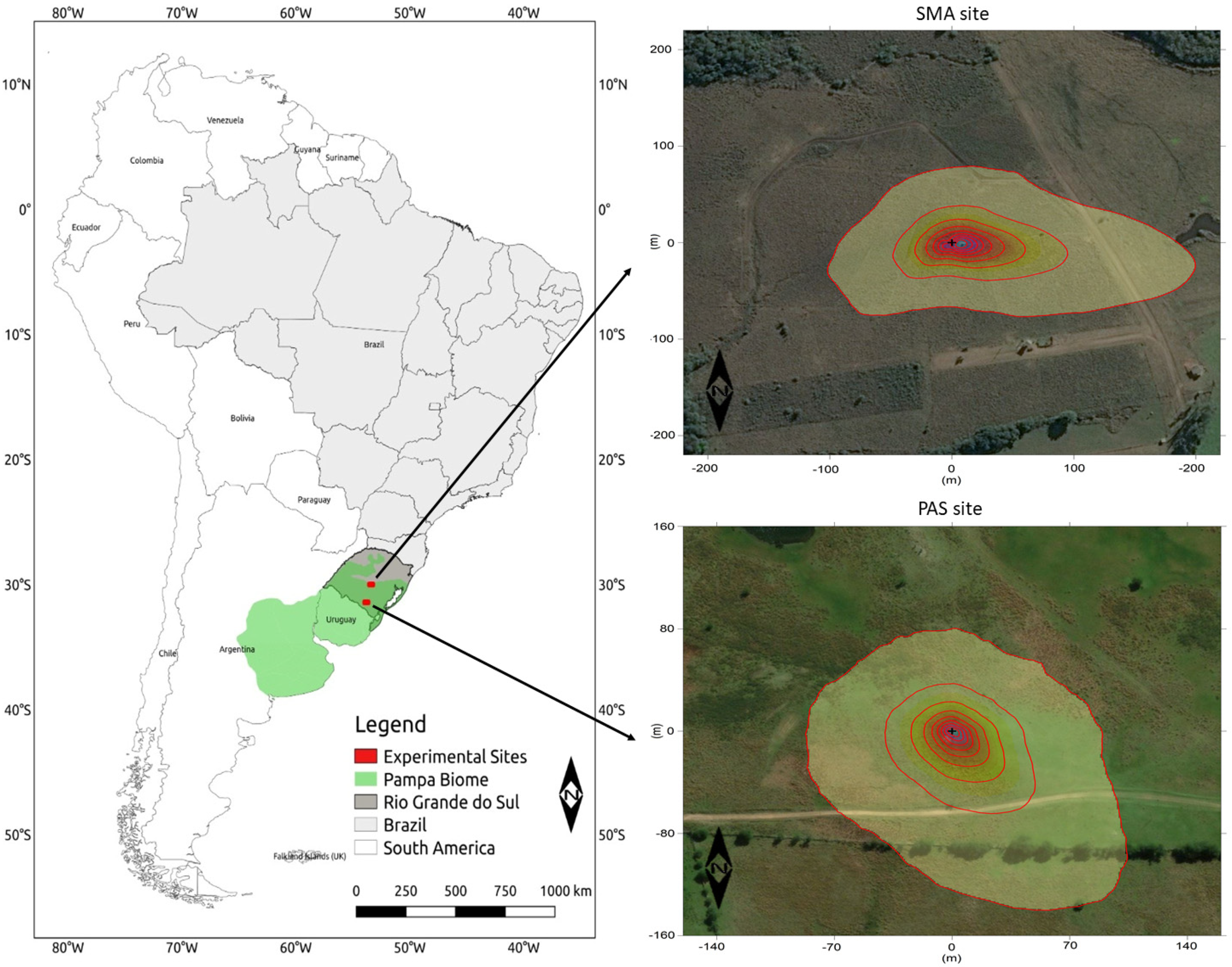
2.1. Site Description

In this study, we analyzed energy surface fluxes and environmental data obtained from two experimental sites, Santa Maria and Pedras Altas, both in the Pampa biome, located in the Rio Grande do Sul state, Brazil (Figure 1). The climate is classified as Cfa, temperate, with hot summer and no dry season, according to the Köppen classification [40]. The vegetation in the Pampa biome is dominated by photosynthetic metabolism C3, but co-exist with C4 species, being one of the distinct characteristics of the South Brazilian grasslands. Both sites are within similar vegetation physiognomies in the Pampa, with a high diversity of grass species used as pasture for cattle.
The Santa Maria site, SMA, (lat 29°43′27.502″ S; lon 53°45′36.097″ W, alt 88 m) is located in the municipality of Santa Maria, in an area of 24 ha of natural vegetation. The soil is classified as Eutrophic Haplossol, according to the exploratory soil map of the state of Rio Grande do Sul [41]. The textural class of soil is clay loam (47.12% sand; 16.90% clay; 35.97% silt), with field capacity, θFC = 0.34 m3 m−3; permanent wilting point θWP = 0.12 m3 m−3; soil porosity, θs = 0.46 m3 m−3; and soil bulk density, ρ s = 1397 kg m−3, measured at 0.5 m depth. The vegetation found in the study area is natural pasture with a predominance of Andropogon lateralis, Axonopus affinis, Paspalum notatum, and Aristida laevis [42], uniformly distributed in the study area [43].
The Pedras Altas site, PAS, (lat 31°43.556′ S; lon 53°32.036′ W, alt 395 m) is located in a private property in the municipality of Pedras Altas-RS. The soil is classified as Neosol and Cambisol [41], with rocky outcrops, and a sandy loam structural classification (59.30% sand; 0.81% clay; 39.89% silt). The soil properties measured at 0.5 m depth are θFC = 0.31 m3 m−3; θWP = 0.03 m3 m−3; soil porosity, θs = 0.44 m3 m−3; and soil bulk density, ρ s = 1405 kg m−3. The phytophysiognomy of the site has a predominance of grassland, mainly stoloniferous and rhizomatous species, such as Axonopus affinis, Paspalum notatun, Aeristida laevis, and Iriantus angustifolium. More information regarding the soil type and vegetation for both sites can be found in Rubert et al. [39].
The phenology of vegetation at both sites was estimated using the EVI (Enhanced Vegetation Index) data time series with a spatial resolution of 250 m obtained from the MODIS sensor (Moderate Resolution Imaging Spectroradiometer, is the instrument aboard the NASA’s Terra satellite) through the product MOD13Q1. The surface albedo was obtained from the MODIS sensor through the product BRDF/MCD43A (MODIS/Terra + Aqua BRDF and calculated albedo (“shortwave actual”), with spatial resolution of 500 m. The selected period was from 29 August 2014 to 15 October 2016, (every 16 days) for EVI and from 29 August 2014 to 7 October 2016, to surface albedo (every 8 days). These data comprise the same period of energy fluxes analyzed in this work.

2.2. Energy Fluxes and Meteorological Measurements

PAS and SMA experimental sites were equipped with flux towers measuring atmospheric variables and surface fluxes. The flux towers were equipped with the sensors described in Table 1. The eddy covariance method (EC) was used to estimate LE and H from 1 September 2014 to 1 September 2016, in both sites. Further details are described in [44,45,46].
The LE and H fluxes were estimated on a half-hour timescale using the EddyPro™ software, version 6.1, Li-Cor (Lincoln, Nebraska, EUA). Turbulent fluctuations were obtained in average per block and double rotation and correction for the effects of density [47]. The high-frequency spectral correction was based on mathematical formulations to model the flux and spectral properties that describe flux attenuations due to the instrumental configuration [48]. High and low pass filter corrections followed the methodology described by Moncrieff et al. [49] and Moncrieff et al. [50], respectively. Quality tests on fluxes followed the methodology described by Mauder and Foken [51]. The angle of attack correction for wind components was determined according to Nakai and Shimoyama [52]. For statistical analysis, the removal of spikes followed the method described by Vickers and Mahrt [53].
Physically inconsistent data were filtered in post-processing. Gaps in the time series of energy fluxes generated by the post-processing step or sensor malfunctions were filled using the method proposed by Reichstein et al. [54] with the REddyProc package. More details regarding the sensors, footprint measurement, surface flux processing, and gap-filling are described in Rubert et al. [39].

2.3. Components of the Energy Balance

The relationship between available energy (RnG) and the turbulent fluxes (H + LE) is often used as an indicator of the H and LE accuracy estimated by the eddy covariance method [55,56,57]. The slope of the linear regression between (RnG) and (H + LE) for the period evaluated was 0.75 for SMA and 0.72 for PAS, as analyzed and discussed by Rubert et al. [39]. In this work, the energy balance closure followed the methodology described by Foken et al. [57], in which the experimental Bowen ratio (β = H/LE) for each site was used to distribute the residual energy, RES, (RES = RnGHLE) between LE and H.
The evapotranspiration process is influenced mainly by the energy available on the surface, atmospheric demand for water vapor, vegetation physiological factors, and resistances imposed on the transfer of water vapor between the vegetation and the atmosphere. The Food and Agriculture Organization (FAO) recommends using the Penman–Monteith method to estimate evapotranspiration, according to the FAO Bulletin 56 [58]. The Penman–Monteith equation combines aerodynamic and thermodynamic aspects to describe water vapor transfer between the surface and the atmosphere. The latent heat flux using the Penman–Monteith equation ( L E P M ) is defined by:
L E P M = ( Δ ( R n G ) + ρ a c p ( e s e a ) r a ( Δ + γ ( 1 + r s r a ) ) )
where R n (W m−2) is the net radiation, G (W m−2) is the soil heat flux, ρ a   (kg m−3) is the mean air density at constant pressure, c p   (J kg−1K−1) is the specific heat of air at constant pressure, e s (kPa) is the saturated water vapor pressure, e a (kPa) is the water vapor pressure of the air, ( e s e a ) (kPa) is the air vapor pressure deficit (VPD), Δ (kPa °C−1) is the slop of the saturation vapor pressure temperature relationship, γ (kPa) is the psychometric constant; r s   (s m−1) is the surface resistance, r a (s m−1) is the aerodynamic resistance. Equation (1) results in hourly average values of L E P M (W m−2). The conversion to daily evapotranspiration (mm d−1) (or hourly (mm h−1)) is done using the daily average (hourly) of L E P M multiplied by the conversion factor of 0.0353 (0.0014). The same procedure is performed with the experimental LE after the energy balance closure to estimate the actual ET. In this work, the surface conductance was indirectly estimated by inverting the Penman-Monteith model (Eq. 1) using LE obtained by EC method:
1 C s = r s = r a γ [ Δ ( R n G ) + ρ a c p C a ( V P D ) L E ( Δ + γ ) ]
Ca, which represents the intensity of vertical turbulence, close to the surface that carries heat and water vapor between the soil surface and the overlying atmosphere, was estimated according to Campbell and Norman [59], correcting the atmospheric stability.
1 C a = r a = 1 u ρ a k [ l n ( z d z o m ) + Ψ m ] [ l n ( z d z o m ) + Ψ m ] [ l n ( z d z o v ) + Ψ v ]
where u is the friction velocity, k is the Von Kármán constant (0.41), z is the height where the wind speed was measured, d is the zero-plane displacement, z o m (m) is the roughness length governing momentum transfer, calculated as 0.1 of the grass height, z o v (m) is the roughness length governing the transfer of heat and vapor, calculated as 0.1 of z o m . Functions Ψ m and Ψ v correspond to the stability correction factors for the momentum and sensible heat, respectively.
The most used method to study atmospheric stability conditions is the stability parameter ζ , as described by Campbell and Norman [59], estimated from the convection rate that produces mechanic turbulence in the air.
ζ = k g z H ρ a c p T e m p ( u ) 3
where g (m s−2) is the gravity acceleration, T e m p (°C) is the air temperature, and others as described above. Stable atmosphere corresponds to positive values of ζ , unstable to negative values of ζ , and atmospheric neutrality to values within the interval 0 <   ζ <│0.0325│ [60].
The equations for functions Ψ m and Ψ v to correct the atmospheric stability proposed by Campbell and Norman [59] are:
-
For atmospheric instability:
Ψ v = 2   l n [ 1 + ( 1 16 ζ ) 1 2 2 ]
Ψ m = 0.6   Ψ v
-
For atmospheric stability:
Ψ m = Ψ v = 6   l n ( 1 + ζ )

3. Results and Discussion

The analysis of the results was separated into two parts: one based on the entire period of data available and the second on two sub-periods, autumn-winter (AW), from April to September, and spring-summer (SS), from October to March.

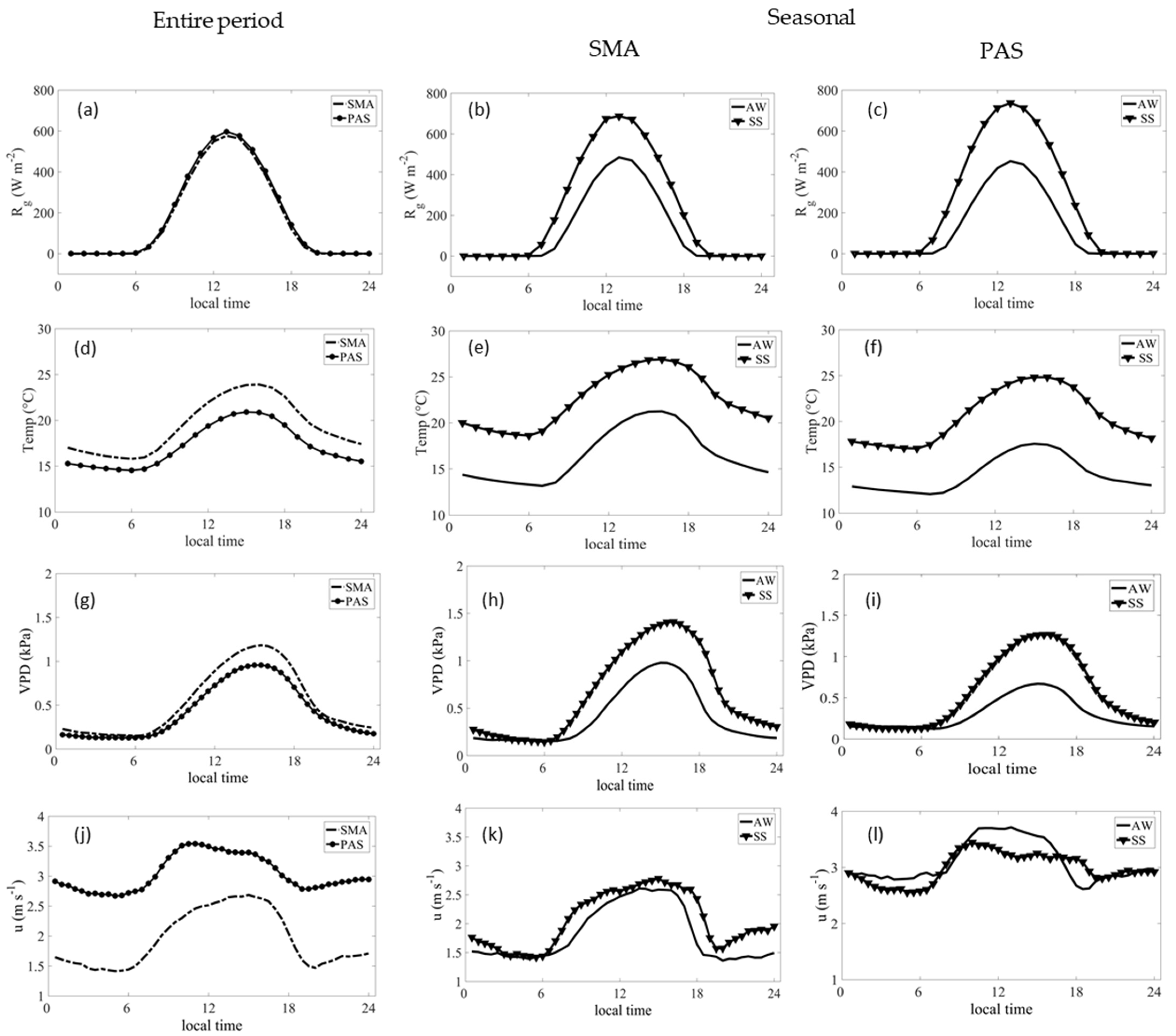
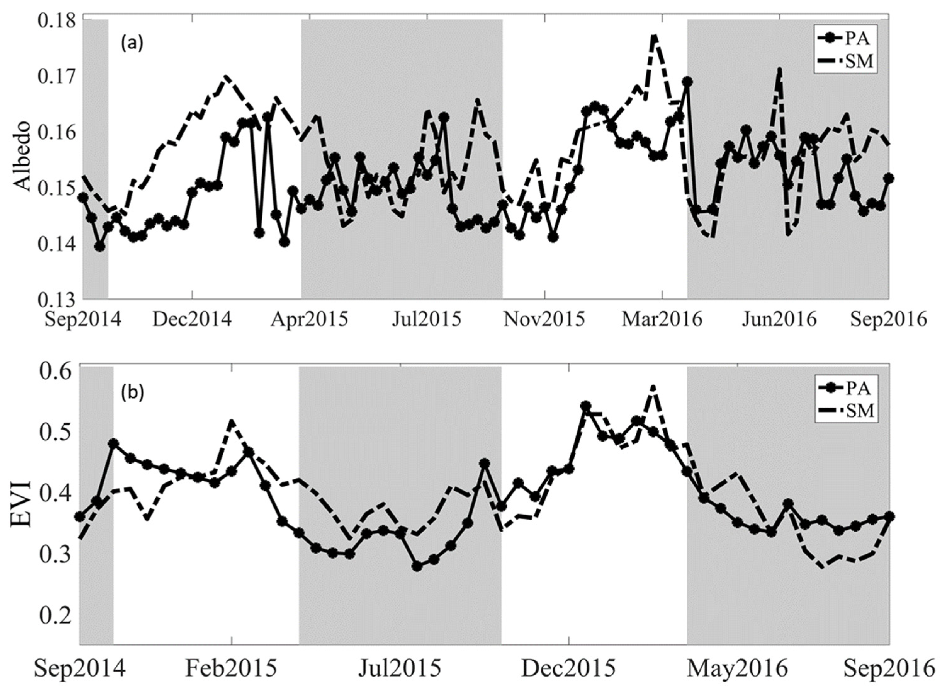
3.1. Meteorological and Surface Conditions

Daily cycle of Rg, Temp, VPD, and wind velocity (u) for SMA and PAS sites are shown in Figure 2. The entire period (two years of data) for Rg is very similar for both sites, with a slight difference in AW and SS, being the values greater in SMA in AW and smaller in SS than PAS values (Table 2). SMA presents higher Temp and VPD throughout the daily cycle than PAS (the same is seen in Table 2 for Temp). u is always stronger in PAS, mainly in night periods; however, the wind speed presents the same pattern in AW and SS for each site. During SS the values of Prec were greater in both sites. In the period 2015/2016 PAS had the lowest accumulated annual precipitation. Despite an accumulated difference in rainfall during some periods, Prec was well distributed throughout the year without water deficit. The soil moisture measurements in SMA showed higher values than in PAS, except for the SS period. As expected, Tsoil was greater in SS. When Tsoil was analyzed for the entire period it presented the same value of 19.3 °C in both sites (Table 2).
Figure 3 shows the surface albedo and the EVI. The mean albedo value was 0.15 for both sites during the analyzed period, with lower values in AW. Maximum values occurred in January, February, and March 2016 (in SS), reaching 0.18 for the SMA site. The average EVI values for this period are very similar between both sites, with 0.39 for SMA and 0.38 for PAS. Seasonality for EVI was more pronounced, showing the influences of the canopy and atmosphere, with minimum values observed in the AW, suggesting a slightly lower photosynthetic activity.

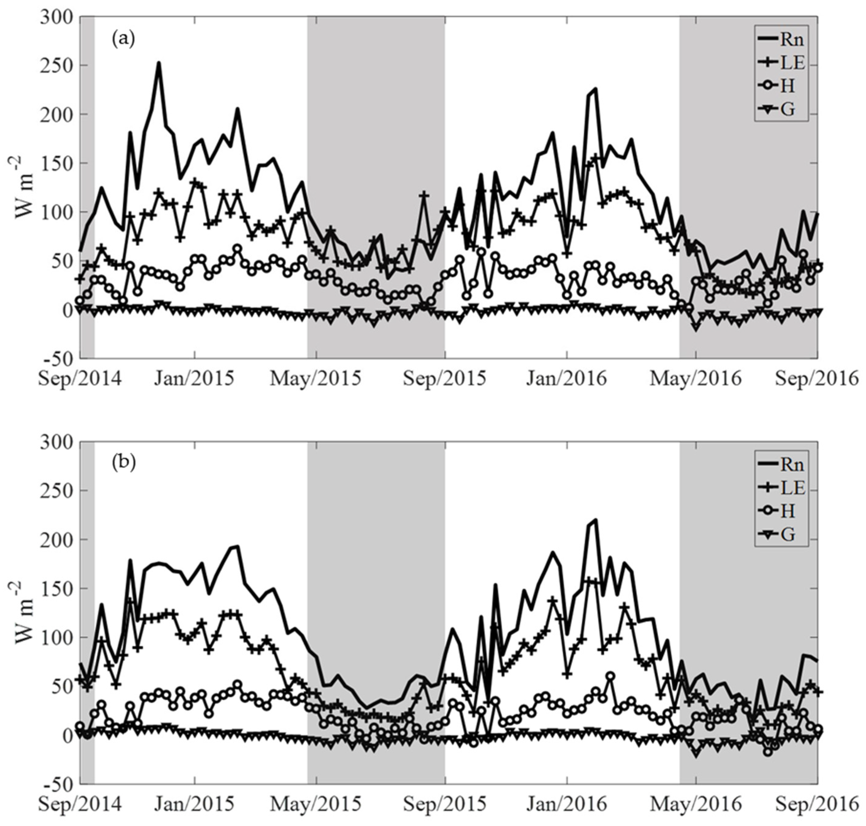
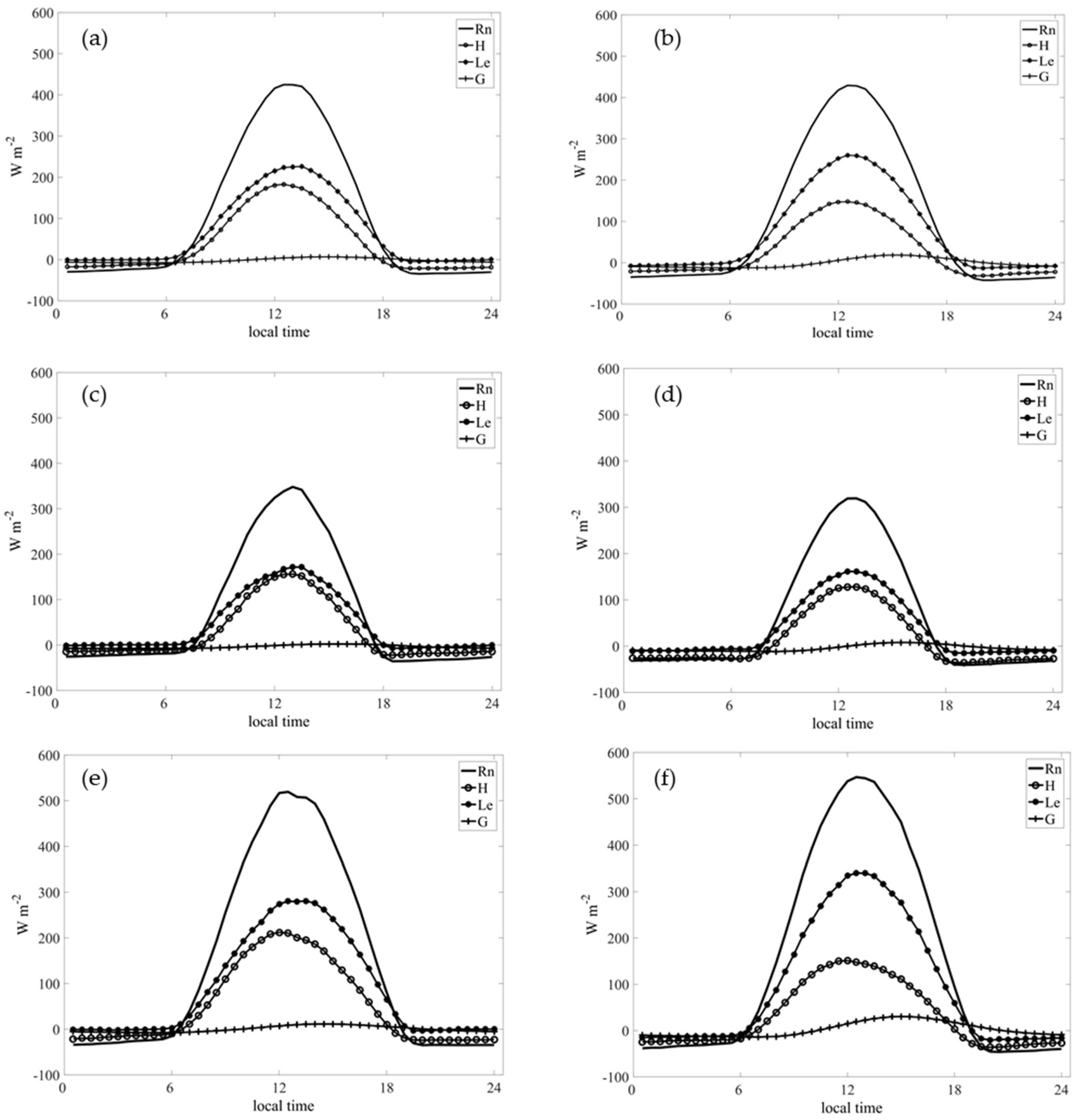
3.2. Energy Balance Components

The seasonal and interannual variability of the energy balance components is presented in Figure 4 and Table 2. A well-characterized seasonal pattern is present in Rn, H, and LE for both sites. Daily variability of Rn, LE, and H was lower in AW and higher in SS. H presented a low amplitude of seasonal variation, while LE presented strong seasonality, similar to Rn.
The annual Rn average presented similar values for both sites (Table 2), Rn values for AW being 47% and 39% smaller than SS in the SMA and PAS sites, respectively. Similar behavior and results were observed for LE. The H values were 62% and 54% smaller in AW than SS for SMA and PAS sites, respectively. Soil heat flux for both sites was generally negative in AW, and close to zero in SS. Therefore, in AW the subsurface heats the surface, while the opposite happens in SS. The smaller energy fluxes in AW are associated with smaller solar radiation in this period (Figure 2 and Table 2), coupled with a decrease in local vegetation (Figure 3) as also reported by Rajan et al. [16], Yunusa et al. [61] and Trepekli et al. [62].
In all analyzed periods, LE was higher than H, being β < 1 for both sites (Table 2). Lower values of β were found in the SS period for each site, while the highest values were found in AW. The PAS presented smaller β values than SMA, with less interannual variability. This difference in the flux partition may be related to the structure of the grassland vegetation at each site. Although the grassland vegetation of the Pampa biome is quite similar throughout the region, the SS is the highest biomass production period in the Pampa [63,64], responding locally to factors such as climate and soil. Thus, vegetation phenology in the Pampa biome also affects energy partitioning.
Figure 5 shows the average daily cycle of the energy balance components (Rn, H, LE, and G) for the SMA and PAS sites. In an annual daily cycle, the net radiation has a daily maximum of 425.0 W m−2 and 429.1 W m−2 for SMA and PAS, respectively. The values are negative between 18:30 and 6:30 local time. Rn was higher in SS, reaching a maximum of 547 W m−2, while in AW, the maximum was 320 W m−2.
LE reached a maximum of 226.3 W m−2 for SMA and 260.2 W m−2 for PAS in an annual daily cycle. Negative LE values were obtained in both sites at night, with more pronounced values for PAS, indicating the occurrence of condensation or dew formation during the night over most of the periods [55,65]. In AW, lower maximum values for LE were observed, reaching 48% and 61% of LE in SS, at the PAS and SMA sites, respectively. LE reverses its signal shortly after Rn. VPD is generally lower during the night when the air is colder, and increases during the day, when the air temperature is higher (Figure 2). LE increases throughout the day, with the beginning of the atmospheric convective processes, controlled by the net radiation. It reaches its maximum with higher air temperatures and decreases from the hottest period of the day due to the vegetation’s biophysical conditions, closing the stomata to avoid water stress to the plants.
H shows little difference between the sites in their maximum and minimum values in the annual daily cycle. Its maximum was 147.6 W m−2 at noon, local time, for PAS and 182.9 W m−2 for SMA. In both sites, the H had a similar behavior between AW and SS. The difference between sites shows little influence of the available energy (RnG) in the range of variation of H. Therefore, we can infer that the turbulence must be produced mainly by mechanical actions in PAS due to the greater wind speed (Figure 2), and less intensity by thermal convection, i.e., less air temperature (Figure 2). Comparing the AW and SS periods, the difference in the maximum amplitude values of H was of the order of 20 W m−2 and 56 W m−2 for the PAS and SMA sites, respectively.
G is near zero through the day in both sites. PAS presents G values slightly higher than the SMA site, possibly due to the soil type, which in PAS is sandy loam, allowing greater soil thermal conduction [66].

3.3. Environmental Variables That Control the H and LE Fluxes

The relationships between the environment variables (Rg, Temp, RH, and VPD) and H and LE for the SMA and PAS sites are shown in Table 3. The turbulent fluxes for both sites had a better correlation to Rn. LE and Rg correlation coefficients for the SMA and PAS sites have very similar values. The LE correlates better with Rg and VPD.
The correlation between energy fluxes and air temperature showed different values for each flux analyzed in this study. For LE, the PAS site showed a better correlation with air temperature when compared to the SMA site, unlike the H, which has a small correlation and very close values for both sites. These results support that air temperature is an indirect controller of evapotranspiration through its effect on the VPD [67].
The results of this study for the Pampa biome showed that local microclimate plays an important role in the energy partition. The increase in Rn increases both H and LE. However, any increase is controlled by water vapor, since the values of Pearson’s correlation coefficients showed that H and LE tend to increase with high evaporative demand (high VPD). Likewise, H and LE raise with the increase in air temperature. Unlike the Pampa biome, Majozi et al. [68], in a similar study over the Savannah biome, reported that the increase in VPD results in an increase in H and a decrease in LE.

3.4. Aerodynamic and Surface Conductances

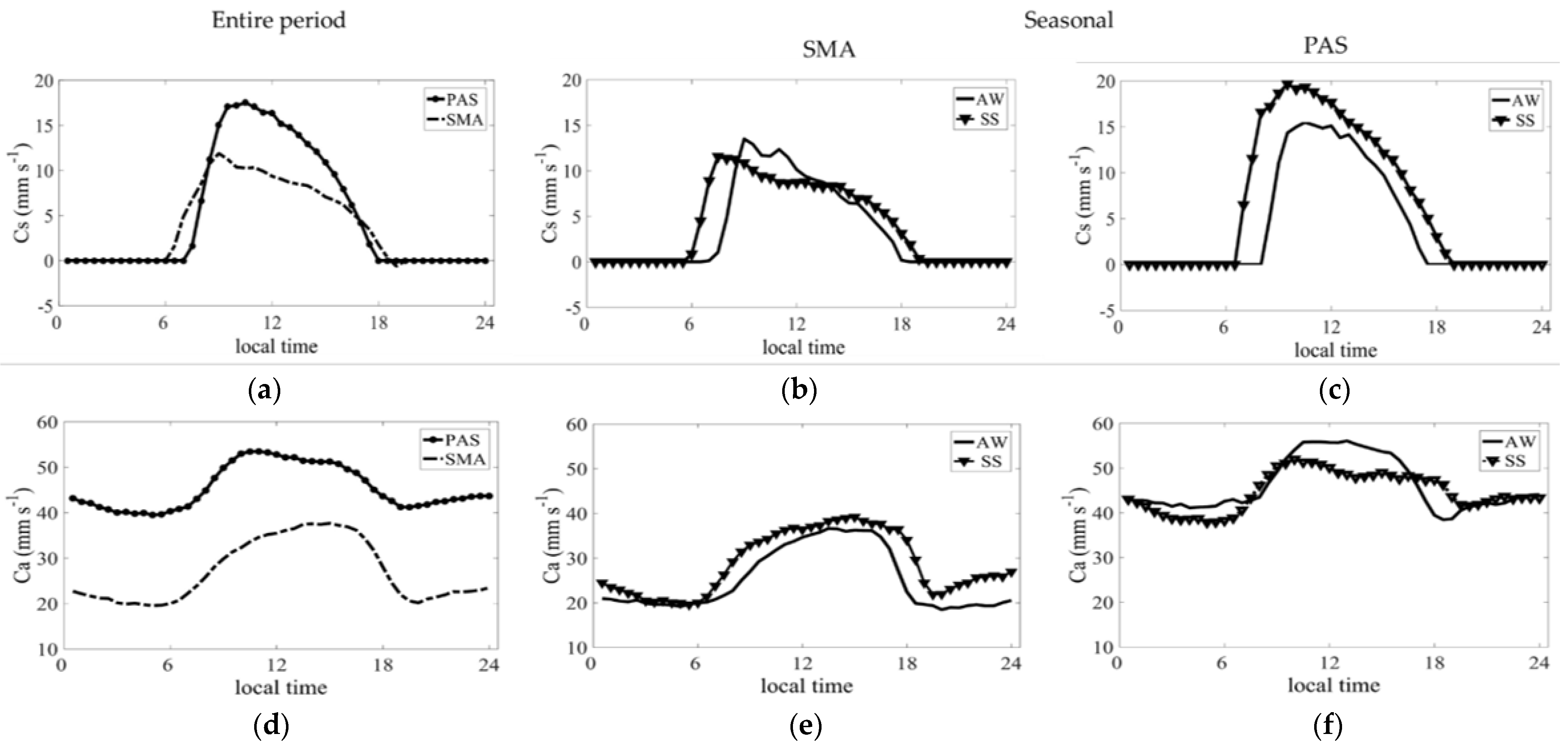
3.4.1. Average Daily Cycles

The average daily cycle of Cs and Ca for the entire study period and AW and SS periods in the Pampa biome are shown in Figure 6. Cs curve pattern has a maximum before noon, of 11.9 mm s−1 and 17.5 mm s−1, in SMA (9:00) and PAS (10:30), respectively. Alves and Pereira [69] reported that the sharp increase of Cs in the early morning hours is due to the stomatal opening caused by solar radiation incidence. In the afternoon, the decrease in Cs is presumably due to stomatal closure, associated with other microclimate variables that directly influence Cs, higher temperatures, and VPD (Figure 2). In a study in the Amazon Forest, Goulden et al. [70] reported a fall in Cs in the afternoon attributed to stomatal closure caused by a high-temperature effect on photosynthetic biochemistry, an intrinsic circadian rhythm, or a combination of the three effects. In the average daily cycle, the highest surface conductance value for PAS is 32% higher than Cs at the SMA site. Krishnan et al. [71] found maximum daily values for surface conductance of 14 mm s−1 in a pasture area in North America. Liu and Feng [72] reported maximum daily values for Cs of 28.3 mm s−1 in degraded pasture areas in China. Wang et al. [73] also found similar Cs values in Australia, 15 mm s−1. Cs was also studied in some Brazilian biomes. Rodrigues et al. [74] obtained a maximum Cs value of 12.6 mm s−1 in the Cerrado. Da Rocha et al. [31] obtained maximum daily values of 25 mm s−1 in a forest biome while Tan et al. [75] suggested for the maximum Cs of tropical forest a value of 24.8 ± 13.8 mm s−1. Marques et al. [76], for Caatinga biome, found a similar behavior for the daily cycle of Cs, but with maximum values (3 and 5 mm s−1) lower than those obtained here (10 and 20 mm s−1).
Negative Cs values were observed before 6:30 and after 18:30 at the SMA site. For the PAS site, Cs has a longer interval, between 07:30 and 17:30, with negative values. According to Groh et al. [77] and Phillips and Oren [78], we assumed that Cs is zero for a wet canopy during the night period. Thus, water evaporates freely at its minimum rate, that is, without resistance to water vapor. When the canopy is dry, Cs is positive. When calculated using flux data from the eddy covariance method, Cs showed greater fluctuations during the day because the data obtained with this method exhibit relatively large fluctuations, especially when the local stability of atmospheric stratification changes in the early morning and late afternoon [57,79].
On average, for the entire study period, Ca reaches its maximum value at 11:00 at the SMA site and 15:00 at the PAS site. There is a significant difference in the peak hours of Ca, which is directly associated with the friction velocity that reaches its highest values at noon at the SMA site and 15:00 in PAS. The maximum values obtained for SMA and PAS are 37.7 mm s−1 and 53.5 mm s−1, respectively, which represents a 30% difference between both sites. The differences in Ca between the sites can be attributed to the different wind speeds (Figure 2) since this variable is the main component in the calculation of aerodynamic conductance.
The analysis of Cs in the AW and SS periods (Figure 6) shows maximum values at the SMA site of 13.5 mm s−1 and 11.6 mm s−1, respectively. In PAS, the values are higher, with 15.5 mm s−1 in AW and 19.7 mm s−1 in SS. Thus, the difference in Cs between the SMA and PAS sites is 13% in the AW period and 42% in the SS period. However, Ca differs between the SMA and PAS sites by 35% and 24% in the AW and SS periods, respectively. The maximum values obtained for Ca at the SMA site are 36.6 mm s−1 and 39.2 mm s−1 in the AW and SS periods, respectively. In PAS, the maximum values obtained are 56.1 mm s−1 in the AW and 52.0 mm s−1 in the SS. These values show a clear seasonal trend related to the weather and climate conditions of the study sites since both have native field ecosystems in the Pampa biome.
Patterns of seasonal variability in Cs and Ca have been observed in other studies, such as in the Amazon Forest [31] and Pantanal [29]. In the Cerrado, Cabral et al. [30] reported that Cs presented a strong seasonal variation of approximately 20 mm s−1 and 2 mm s−1 in rainy and dry seasons, respectively. However, Ca showed relatively small seasonal variation and the average between the dry and rainy seasons was 129 mm s−1. Krishnan et al. [71] reported a significant seasonal and interannual variation in Cs similar to the changes that occurred in ET for pastures in North America.
In the AW and SS periods, Cs and Ca were directly related to the wind intensity, as verified by comparing Figure 6 and the different atmospheric variables presented in the average daytime cycle in Figure 2. Cs, which can be considered analogous to stomatal conductance, on a large scale, provides a useful measure of the effect of energy exchanges on plant physiology. Cs at the SMA site was higher in the AW period (Figure 6), which suggests that seasonal changes in Cs are strongly associated, in part, with changes in the leaf area index (LAI) or leaf physiology. The water flux between the leaf and atmosphere is high since the AW period tends to show no water restrictions at the site and the environmental conditions for the exchange of gases in the stomata are favorable.
Cs at the PAS site had its highest value in the SS period, which is consistent with the higher wind velocity in the AW and SS periods. The transfer of steam inside the canopy depends on the intensity of the wind, or indirectly on Ca, which, according to Grelle et al. [80], is a function of turbulence parameters. Higher values in the wind velocity are also favorable to the increase of evapotranspiration since the water vapor transfer process is facilitated due to the increase in Ca [81]. High wind velocity decreases the thickness of the boundary layer, allowing the stomatal resistance to control water loss. If the water in the soil (soil moisture) is less abundant, as is the case in PAS all year (Table 2), the stomata will open less or even remain closed on a sunny morning. Finally, the theory used to estimate the conductances, the “big-leaf” theory, combined with the method of estimating turbulent fluxes, eddy covariance, couples the plant surface with the atmosphere. Thus, vegetation cover near surface perceives the direct effects of turbulence during the day. Therefore, there is a need to develop empirical models that contemplate not only plant physiology (through stomata) but also a model that responds to all factors that control stomatal conductance.

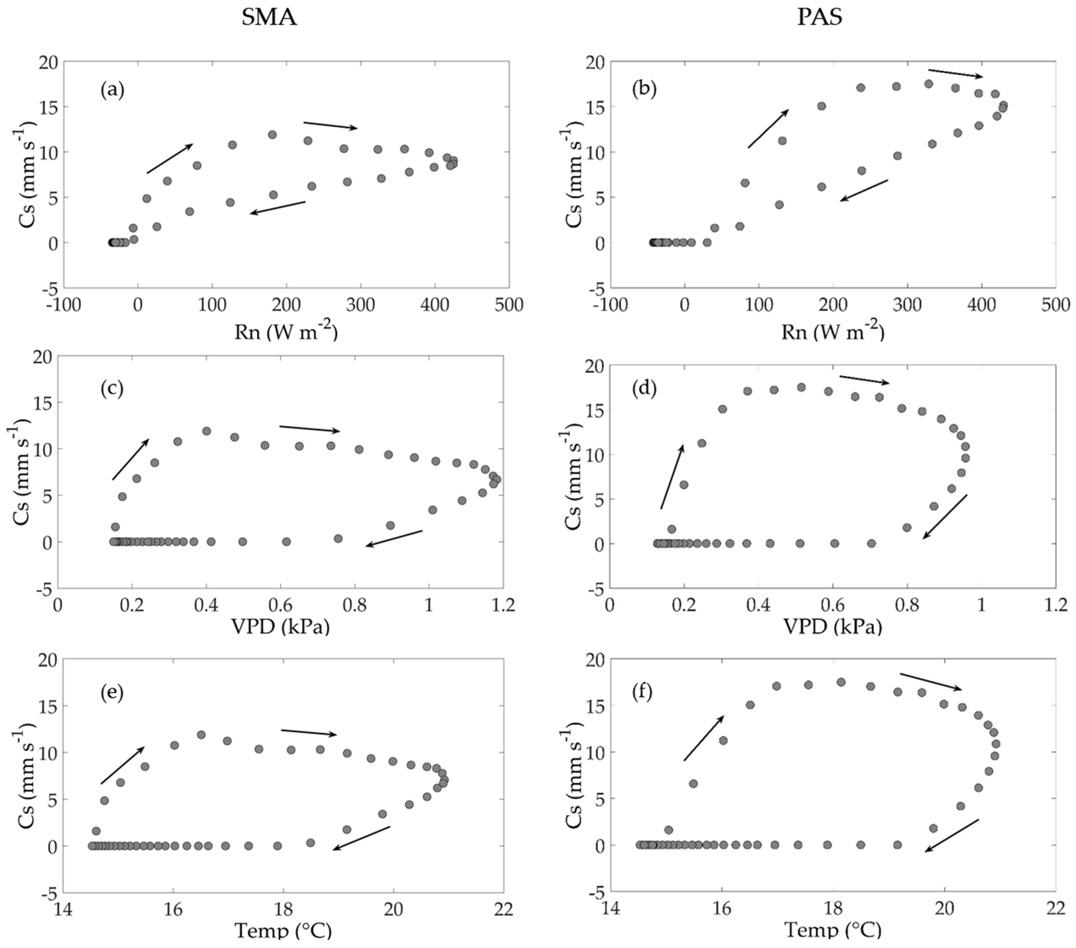
3.4.2. Hysteresis Loops in the Surface Conductance

Cs responses to the main environmental variables (Rn, VPD, and Temp) for the average daily cycle throughout the study period are shown in Figure 7. These relationships form hysteresis loops, which had the directions followed in a clockwise direction for the three meteorological variables in both sites. The Cs values increased linearly in the morning, with an increase in Rn, VPD, and Temp at both sites. Table 4 shows the hour in which the hysteresis loops occurred for the meteorological variables at the maximum peak of the surface conductance. When reaching the maximum Cs peak, the available energy had not yet reached its maximum value. In other words, Cs decreased at midday with the increase in Rn. Cs decreases linearly with the decrease in Rn to its lowest value in the afternoon, reaching negative values at night.
The regressions between Cs and the environmental variables (Rn, VPD, and Temp) were determined to identify the main influencing factors on the surface conductance on a daily scale throughout the study period. The Pearson’s coefficients are presented in Table 5. Rn was the main influencing factor controlling Cs in the morning (P1—Table 5). However, the significant influence of air temperature on the surface conductance in the P1 period must be considered. The VPD and morning temperature directly influence the surface conductance in the afternoon. Therefore, we can infer that the behavior of opening or closing stomata can also contribute to the emergence of hysteresis.
The gaps between the meteorological variables and Cs of the Pampa biome were more prominent at the PAS site. Cs in the afternoon (P2) was more linearly correlated with VPD and Temp, r = −1 and r = −0.99, respectively, which provides us with another important relationship to verify the limiting causes of Cs. While VPD or Temp increases, Cs tends to decrease since stomata must regulate their opening to prevent dehydration [82]. This fact is already known. However, the factors and intensities of these responses still require investigation. If there is a stomatal response to VPD, the mechanism that causes this response is still controversial [83]. According to Streck [83], two hypotheses proposed for this mechanism are discussed in the scientific community. The first, feedforward, is that stomatal conductance (Ce) decreases directly with the increase in VPD, with abscisic acid as the signal for the response. In the second hypothesis, feedback, Ce decreases with the increase in VPD due to the increase in leaf transpiration, which decreases the water potential in the leaf. Kelliher [84] reports that vegetation with LAI > 3 m2 m−2 has minimal soil evaporation, allowing Cs to be a good approximation of the physiological parameter Ce. Thus, in this work, it was possible to verify the effect of VPD on the daily cycles of surface conductance and, in turn, the stomatic response to atmospheric demand.
The plant can undergo water stress with high VPD. Therefore, the stomata close in response to VPD as a self-protective mechanism to avoid high transpiration rates [85]. The Pampa vegetation, which had good water availability throughout the period [39], presented a decrease in Cs throughout the day just after 9:00 when Rn, Temp, and VPD have not yet reached their maximum values. In other words, the period in which the stomatal opening became narrower (Cs decreasing) was before the decline in meteorological variables. This was also reported in other studies [86,87,88], showing what directly caused the hysteresis loops between Cs and the weather variables during the day. Even so, explaining the causes of this phenomenon seems to be fraught with complex interactions between exogenous and endogenous factors for the plant system [89,90]. The stomatal response to VPD is still a subject of research in plant physiology [83].

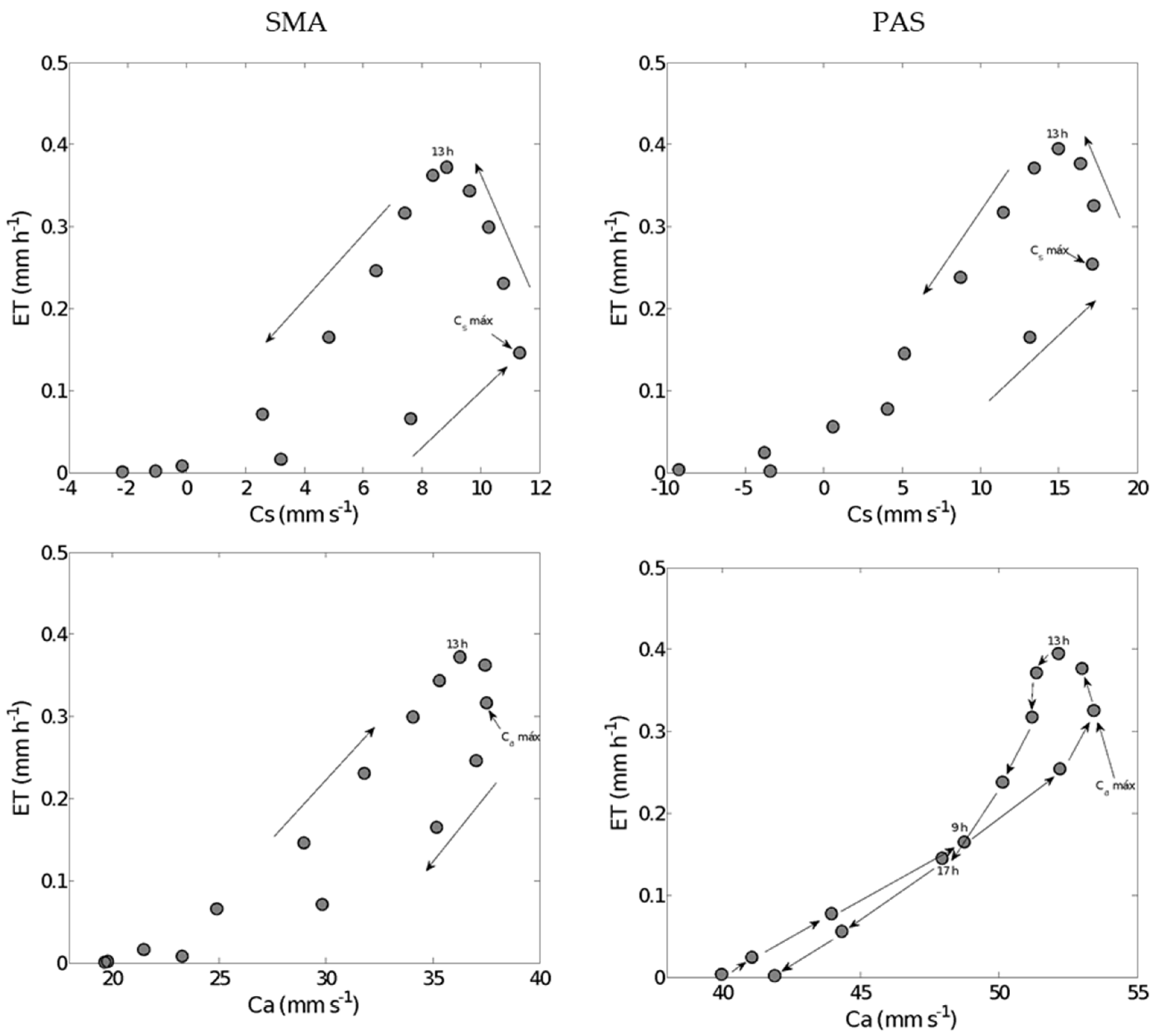
3.5. Biophysical Control of Evapotranspiration

The relationships between Cs and Ca also formed hysteresis loops with ET in the average daily cycle and are shown in Figure 8. The relationship between Ca and ET for the PAS site showed a different behavior from the other relationships. In this cycle, the ET response to Ca increase is high in the early morning. The same occurs after 17:00 when the ET drop ratio shows a quick response due to the Ca decrease. In other words, the hysteresis cycle may be negligible during these periods. Between 9:00 and 17:00, the formation of hysteresis loops between ET and Ca is counterclockwise and shows ET response to Ca when aerodynamic conductance values are already reducing. At 9:00 and 17:00, the ET reaches close values, ending the hysteresis cycle. At the SMA site, the relationship between aerodynamic conductance and ET forms clockwise hysteresis loops, showing that the ET response to Ca is high earlier in the day. At 13:00 (local time), the maximum ET value begins to drop the Ca, thereby decreasing ET. However, in this period, the ET response to Ca is lower when compared to the morning period. Therefore, between 13:00 and 15:00, ET shows less Ca dependence, showing high biophysical control in the evapotranspiration rate. Mallick et al. [91] report hysteresis loops between the Cs and Ca with evaporation and transpiration in the Amazon Basin. The authors reported significant hysteresis between the transpiration component and Cs during the dry season for sites with pasture vegetation. The evaporation component was significantly influenced by Ca for all sites.
The relationships between ET and surface conductance for both sites formed hysteresis loops in a counterclockwise direction, showing a low ET response in the morning. In this period, ET increases as Cs increases until reaching their maximum value at 9:00 at the SMA site and 11:00 in PAS. After this time, Cs begins to decrease with the increase in ET. Therefore, ET responds to Cs in this interval since evapotranspiration does not reduce instantly, even after the stomata have closed. In summary, the decrease in ET is mainly caused by the Cs reduction response due to the increase in VPD and air temperature.
The areas of the hysteresis curves were estimated to verify the intensity of ET response to Cs and Ca. Hysteresis was weaker in the ET-Ca ratios when compared to ET-Cs. The largest area obtained was for the ET-Cs ratio at the SMA site (0.0657), 33% higher than for the PAS site. The ET-Ca ratio was weaker at the PAS site, representing only 7% of the area’s value for the same ratio at the SMA site. On average, ET responds more strongly to surface conductance, about 86%, compared to the Pampa biome ET-Ca ratio.

4. Conclusions

In this work, we assessed the patterns and controls in the turbulent energy exchanges of the Pampa biome in southern Brazil from two grassland sites. Rn presented a strong seasonality, with AW being 47% and 39% smaller than SS in the SMA and PAS sites, respectively. LE was the main component of the energy balance in AW and SS periods, but with similar results of H during AW in both sites. Global radiation was the main controller of the LE and H. G was a smaller component of the energy partition, with greater values in PAS.
Cs and Ca for both sites did not show seasonality. Cs and Ca were highly influenced by u and turbulence conditions in each site. Rn was the main driving factor controlling Cs in the morning. VPD and morning air temperature directly influenced Cs in the afternoon. Cs presented a similar daily cycle for both sites, with Ca showing a higher magnitude in PAS, mainly because of higher u . The hysteresis cycles formed by ET and the conductances showed substantial biophysical control in the ET process complex.
Cs and Ca are considered complex variables and have fundamental importance in most land surface models. In addition, the Pampa biome is a complex ecosystem where the surface–atmosphere interactions depend on weather and climate, soil, and vegetation phenology. Thus, the results presented in this study should guide numerical modeling simulations and public water use policies for Pampa biome ecosystem.

Author Contributions

G.C.D.R., V.d.A.S., T.Z., G.P.V., A.M. and T.B. collected, processed, and analyzed the eddy covariance data. G.C.D.R. and D.R.R. wrote the manuscript. D.R.R. and L.G.G.d.G. conceived and designed the experiments. D.R.R. supervised and advised all the research work that led to this paper. D.R.R., V.d.A.S., T.B., A.R. and L.G.G.d.G. reviewed the manuscript and conducted the English editing. All authors have read and agreed to the published version of the manuscript.

Funding

This study was financed in part by Coordination for the Improvement of Higher Education Personal (CAPES-Brazil) through the project CAPES-ANA-DPB (88881.178688/2018-01).

Institutional Review Board Statement

Not applicable.

Informed Consent Statement

Not applicable.

Acknowledgments

The authors acknowledge the National Council for Scientific and Technological Development (CNPq-Brazil), the Coordination for the Improvement of Higher Education Personnel (CAPES-Brazil), the Foundation for Research of Rio Grande do Sul State (FAPERGS, Project n° 17/2551-0001124-4), and Financier of Studies and Projects (FINEP-Brazil) for their financial support. The authors acknowledge the staff of the Micrometeorology Lab of the Federal University of Santa Maria (UFSM) for the technical support provided, particularly relative to the flux tower and the eddy covariance instruments. The authors acknowledge the Acevedo family for allowing us to carry out the experiment on their farm in Pedras Altas.

Conflicts of Interest

The authors declare no conflict of interest.

References

  1. Sellers, P.J.; Bounoua, L.; Collatz, G.J.; Randall, D.A.; Dazlich, D.A.; Los, S.O.; Berry, J.A.; Fung, I.; Tucker, C.J.; Field, C.B.; et al. Comparison of Radiative and Physiological Effects of Doubled Atmospheric CO2 on Climate. Science 1996, 271, 1402–1406. [Google Scholar] [CrossRef]
  2. Zhang, Y.; Kadota, T.; Ohata, T.; Oyunbaatar, D. Environmental controls on evapotranspiration from sparse grassland in Mongolia. Hydrol. Process. 2007, 21, 2016–2027. [Google Scholar] [CrossRef]
  3. Woodward, F.I.; Smith, T.M. Global Photosynthesis and Stomatal Conductance: Modelling the Controls by Soil and Climate. Adv. Bot. Res. 1994, 20, 1–41. [Google Scholar]
  4. Adams, J.M.; Faure, H.; Faure-Denard, L.; McGlade, J.M.; Woodward, F.I. Increases in terrestrial carbon storage from the Last Glacial Maximum to the present. Nature 1990, 348, 711–714. [Google Scholar] [CrossRef]
  5. Roesch, L.F.W.; Vieira, F.C.B.; Pereira, V.A.; Schünemann, A.L.; Teixeira, I.F.; Senna, A.J.T.; Stefenon, V.M. The Brazilian Pampa: A fragile biome. Diversity 2009, 1, 182–198. [Google Scholar] [CrossRef]
  6. Overbeck, G.; Muller, S.; Fidelis, A.; Pfadenhauer, J.; Pillar, V.; Blanco, C.; Boldrini, I.; Both, R.; Forneck, E. Brazil’s neglected biome: The South Brazilian Campos. Perspect. Plant Ecol. Evol. Syst. 2007, 9, 101–116. [Google Scholar] [CrossRef]
  7. Ruviaro, C.F.; de Léis, C.M.; Lampert, V.D.N.; Barcellos, J.O.J.; Dewes, H. Carbon footprint in different beef production systems on a southern Brazilian farm: A case study. J. Clean. Prod. 2015, 96, 435–443. [Google Scholar] [CrossRef] [Green Version]
  8. Pillar, V.D.; Müller, S.C.; Castilhos, Z.M.; Jacques, A.V.Á. Campos Sulinos—Conservação E Uso Sustentável Da Biodiversidade; Ministério do Meio Ambiente: Brasília, Brazil, 2009; ISBN 978-85-7738-117-3.
  9. Oliveira, T.E.D.; Freitas, D.S.D.; Gianezini, M.; Ruviaro, C.F.; Zago, D.; Mércio, T.Z.; Dias, E.A.; Lampert, V.D.N.; Barcellos, J.O.J. Agricultural land use change in the Brazilian Pampa Biome: The reduction of natural grasslands. Land Use Policy 2017, 63, 394–400. [Google Scholar] [CrossRef]
  10. Chen, S.; Chen, J.; Lin, G.; Zhang, W.; Miao, H.; Wei, L.; Huang, J.; Han, X. Energy balance and partition in Inner Mongolia steppe ecosystems with different land use types. Agric. For. Meteorol. 2009, 149, 1800–1809. [Google Scholar] [CrossRef]
  11. Babel, W.; Biermann, T.; Coners, H.; Falge, E.; Seeber, E.; Ingrisch, J.; Schleuß, P.-M.; Gerken, T.; Leonbacher, J.; Leipold, T.; et al. Pasture degradation modifies the water and carbon cycles of the Tibetan highlands. Biogeosciences 2014, 11, 6633–6656. [Google Scholar] [CrossRef] [Green Version]
  12. Lan, X.; Li, Y.; Shao, R.; Chen, X.; Lin, K.; Cheng, L.; Gao, H.; Liu, Z. Vegetation controls on surface energy partitioning and water budget over China. J. Hydrol. 2021, 600, 125646. [Google Scholar] [CrossRef]
  13. Lang, Y.; Yang, X.; Cai, H. Assessing the degradation of grassland ecosystems based on the advanced local net production scaling method—The case of Inner Mongolia, China. Land Degrad. Dev. 2021, 32, 559–572. [Google Scholar] [CrossRef]
  14. Knapp, A.K.; Smith, M.D. Variation Among Biomes in Temporal Dynamics of Aboveground Primary Production. Science 2001, 291, 481–484. [Google Scholar] [CrossRef] [Green Version]
  15. Guo, D.; Westra, S.; Maier, H.R. Impact of evapotranspiration process representation on runoff projections from conceptual rainfall-runoff models. Water Resour. Res. 2017, 53, 435–454. [Google Scholar] [CrossRef]
  16. Rajan, N.; Maas, S.J.; Cui, S. Extreme drought effects on summer evapotranspiration and energy balance of a grassland in the Southern Great Plains. Ecohydrology 2015, 8, 1194–1204. [Google Scholar] [CrossRef]
  17. Wang, K.; Dickinson, R.E. A review of global terrestrial evapotranspiration: Observation, modeling, climatology, and climatic variability. Rev. Geophys. 2012, 50, RG2005. [Google Scholar] [CrossRef]
  18. Bonan, G.B. Forests and Climate Change: Forcings, Feedbacks, and the Climate Benefits of Forests. Science 2008, 320, 1444–1449. [Google Scholar] [CrossRef] [Green Version]
  19. Senay, G.B.; Leake, S.; Nagler, P.L.; Artan, G.; Dickinson, J.; Cordova, J.T.; Glenn, E.P. Estimating basin scale evapotranspiration (ET) by water balance and remote sensing methods. Hydrol. Process. 2011, 25, 4037–4049. [Google Scholar] [CrossRef]
  20. Forzieri, G.; Alkama, R.; Miralles, D.G.; Cescatti, A. Satellites reveal contrasting responses of regional climate to the widespread greening of Earth. Science 2017, 356, 1180–1184. [Google Scholar] [CrossRef] [Green Version]
  21. Liu, Z.; Cheng, L.; Zhou, G.; Chen, X.; Lin, K.; Zhang, W.; Chen, X.; Zhou, P. Global Response of Evapotranspiration Ratio to Climate Conditions and Watershed Characteristics in a Changing Environment. J. Geophys. Res. Atmos. 2020, 125, e2020JD032371. [Google Scholar] [CrossRef]
  22. Zha, T.; Li, C.; Kellomäki, S.; Peltola, H.; Wang, K.-Y.; Zhang, Y. Controls of Evapotranspiration and CO2 Fluxes from Scots Pine by Surface Conductance and Abiotic Factors. PLoS ONE 2013, 8, e69027. [Google Scholar]
  23. Igarashi, Y.; Kumagai, T.; Yoshifuji, N.; Sato, T.; Tanaka, N.; Tanaka, K.; Suzuki, M.; Tantasirin, C. Environmental control of canopy stomatal conductance in a tropical deciduous forest in northern Thailand. Agric. For. Meteorol. 2015, 202, 1–10. [Google Scholar] [CrossRef]
  24. Hirano, T.; Suzuki, K.; Hirata, R. Energy balance and evapotranspiration changes in a larch forest caused by severe disturbance during an early secondary succession. Agric. For. Meteorol. 2017, 232, 457–468. [Google Scholar] [CrossRef]
  25. Zhao, W.; Liu, B.; Chang, X.; Yang, Q.; Yang, Y.; Liu, Z.; Cleverly, J.; Eamus, D. Evapotranspiration partitioning, stomatal conductance, and components of the water balance: A special case of a desert ecosystem in China. J. Hydrol. 2016, 538, 374–386. [Google Scholar] [CrossRef]
  26. Yue, P.; Zhang, Q.; Zhang, L.; Li, H.; Yang, Y.; Zeng, J.; Wang, S. Long-term variations in energy partitioning and evapotranspiration in a semiarid grassland in the Loess Plateau of China. Agric. For. Meteorol. 2019, 278, 107671. [Google Scholar] [CrossRef]
  27. Baldocchi, D. A comparative study of mass and energy exchange rates over a closed C3 (wheat) and an open C4 (corn) crop: II. CO2 exchange and water use efficiency. Agric. For. Meteorol. 1994, 67, 291–321. [Google Scholar] [CrossRef]
  28. Jarvis, P.G.; McNaughton, K.G. Stomatal Control of Transpiration: Scaling Up from Leaf to Region. Adv. Ecol. Res. 1986, 15, 1–49. [Google Scholar]
  29. Fraga, C.I.D.M.; Sanches, L.; Pinto Junior, O.B.; Curado, L.F.A.; Gaio, D.C. Canopy Conductance, Aerodynamic Conductance and the Decoupling Coefficient in the Vochysia Divergens Pohl (Vochysiaceae) Forest in the Brazilian Pantanal. Rev. Bras. Meteorol. 2015, 30, 275–284. [Google Scholar] [CrossRef]
  30. Cabral, O.M.R.; da Rocha, H.R.; Gash, J.H.; Freitas, H.C.; Ligo, M.A.V. Water and energy fluxes from a woodland savanna (cerrado) in southeast Brazil. J. Hydrol. Reg. Stud. 2015, 4, 22–40. [Google Scholar] [CrossRef] [Green Version]
  31. da Rocha, H.R.; Goulden, M.L.; Miller, S.D.; Menton, M.C.; Pinto, L.D.V.O.; de Freitas, H.C.; e Silva Figueira, A.M. Seasonality Of Water And Heat Fluxes Over A Tropical Forest In Eastern Amazonia. Ecol. Appl. 2004, 14, 22–32. [Google Scholar] [CrossRef]
  32. Eamus, D.; Cole, S. Diurnal and Seasonal Comparisons of Assimilation, Phyllode Conductance and Water Potential of Three Acacia and One Eucalyptus Species in the Wet-Dry Tropics of Australia. Aust. J. Bot. 1997, 45, 275. [Google Scholar] [CrossRef]
  33. Wilson, K.B.; Baldocchi, D.D. Seasonal and interannual variability of energy fluxes over a broadleaved temperate deciduous forest in North America. Agric. For. Meteorol. 2000, 100, 1–18. [Google Scholar] [CrossRef]
  34. Yu, G.-R.; Nakayama, K.; Lu, H.-Q. Responses of Stomatal Conductance in Field-grown Maize Leaves to Certain Environmental Factors over a Long Term. J. Agric. Meteorol. 1996, 52, 311–320. [Google Scholar] [CrossRef]
  35. Wright, I.R.; Manzi, A.O.; da Rocha, H.R. Surface conductance of Amazonian pasture: Model application and calibration for canopy climate. Agric. For. Meteorol. 1995, 75, 51–70. [Google Scholar] [CrossRef]
  36. Sellers, P.J.; Randall, D.A.; Collatz, G.J.; Berry, J.A.; Field, C.B.; Dazlich, D.A.; Zhang, C.; Collelo, G.D.; Bounoua, L. A Revised Land Surface Parameterization (SiB2) for Atmospheric GCMS. Part I: Model Formulation. J. Clim. 1996, 9, 676–705. [Google Scholar] [CrossRef]
  37. Villalobos, F.J.; Testi, L.; Orgaz, F.; García-Tejera, O.; Lopez-Bernal, A.; González-Dugo, M.V.; Ballester-Lurbe, C.; Castel, J.R.; Alarcón-Cabañero, J.J.; Nicolás-Nicolás, E.; et al. Modelling canopy conductance and transpiration of fruit trees in Mediterranean areas: A simplified approach. Agric. For. Meteorol. 2013, 171–172, 93–103. [Google Scholar] [CrossRef]
  38. Polhamus, A.; Fisher, J.B.; Tu, K.P. What controls the error structure in evapotranspiration models? Agric. For. Meteorol. 2013, 169, 12–24. [Google Scholar] [CrossRef]
  39. Rubert, G.C.; Roberti, D.R.; Pereira, L.S.; Quadros, F.L.F.; Velho, H.F.D.C.; Moraes, O.L.L.D. Evapotranspiration of the Brazilian Pampa Biome: Seasonality and Influential Factors. Water 2018, 10, 1864. [Google Scholar] [CrossRef] [Green Version]
  40. Peel, M.C.; Finlayson, B.L.; McMahon, T.A. Updated world map of the Köppen-Geiger climate classification. Hydrol. Earth Syst. Sci. 2007, 11, 1633–1644. [Google Scholar] [CrossRef] [Green Version]
  41. IBGE. Mapas. Available online: http://mapas.ibge.gov.br/tematicos/solos (accessed on 26 June 2021).
  42. dos Santos, A.B.; de Quadros, F.L.F.; Confortin, A.C.C.; Seibert, L.; Ribeiro, B.S.M.R.; Severo, P.D.O.; Casanova, P.T.; Machado, G.K.G. Morfogênese de gramíneas nativas do Rio Grande do Sul (Brasil) submetidas a pastoreio rotativo durante primavera e verão. Ciência Rural 2014, 44, 97–103. [Google Scholar] [CrossRef] [Green Version]
  43. Quadros, F.L.F.; Pillar, V.D.P. Dinâmica vegetacional em pastagem natural submetida a tratamentos de queima e pastejo. Ciência Rural 2001, 31, 863–868. [Google Scholar] [CrossRef] [Green Version]
  44. Timm, A.U.; Roberti, D.R.; Streck, N.A.; de Gonçalves, L.G.G.; Acevedo, O.C.; Moraes, O.L.; Moreira, V.S.; Degrazia, G.A.; Ferlan, M.; Toll, D.L. Energy Partitioning and Evapotranspiration over a Rice Paddy in Southern Brazil. J. Hydrometeorol. 2014, 15, 1975–1988. [Google Scholar] [CrossRef]
  45. Diaz, M.B.; Roberti, D.R.; Carneiro, J.V.; Souza, V.D.A.; de Moraes, O.L.L. Dynamics of the superficial fluxes over a flooded rice paddy in southern Brazil. Agric. For. Meteorol. 2019, 276–277, 107650. [Google Scholar] [CrossRef]
  46. Acevedo, O.C.; Moraes, O.L.L.; Degrazia, G.A.; Medeiros, L.E. Intermittency and the exchange of scalars in the nocturnal surface layer. Bound.-Layer Meteorol. 2006, 119, 41–55. [Google Scholar] [CrossRef]
  47. Webb, E.K.; Pearman, G.I.; Leuning, R. Correction of flux measurements for density effects due to heat and water vapour transfer. Q. J. R. Meteorol. Soc. 1980, 106, 85–100. [Google Scholar] [CrossRef]
  48. Gash, J.H.C.; Culf, A.D. Applying a linear detrend to eddy correlation data in realtime. Bound.-Layer Meteorol. 1996, 79, 301–306. [Google Scholar] [CrossRef]
  49. Moncrieff, J.B.; Massheder, J.M.; de Bruin, H.; Elbers, J.; Friborg, T.; Heusinkveld, B.; Kabat, P.; Scott, S.; Soegaard, H.; Verhoef, A. A system to measure surface fluxes of momentum, sensible heat, water vapour and carbon dioxide. J. Hydrol. 1997, 188–189, 589–611. [Google Scholar] [CrossRef]
  50. Moncrieff, J.; Clement, R.; Finnigan, J.; Meyers, T. Averaging, Detrending, and Filtering of Eddy Covariance Time Series. In Handbook of Micrometeorology; Kluwer Academic Publishers: Dordrecht, The Netherlands, 2004; pp. 7–31. [Google Scholar]
  51. Mauder, M.; Foken, T. Impact of post-field data processing on eddy covariance flux estimates and energy balance closure. Meteorol. Z. 2006, 15, 597–609. [Google Scholar] [CrossRef]
  52. Nakai, T.; Shimoyama, K. Ultrasonic anemometer angle of attack errors under turbulent conditions. Agric. For. Meteorol. 2012, 162–163, 14–26. [Google Scholar] [CrossRef] [Green Version]
  53. Vickers, D.; Mahrt, L. Quality control and flux sampling problems for tower and aircraft data. J. Atmos. Ocean. Technol. 1997, 14, 512–526. [Google Scholar] [CrossRef]
  54. Reichstein, M.; Falge, E.; Baldocchi, D.; Papale, D.; Aubinet, M.; Berbigier, P.; Bernhofer, C.; Buchmann, N.; Gilmanov, T.; Granier, A.; et al. On the separation of net ecosystem exchange into assimilation and ecosystem respiration: Review and improved algorithm. Glob. Chang. Biol. 2005, 11, 1424–1439. [Google Scholar] [CrossRef]
  55. Wilson, K.B.; Baldocchi, D.D.; Aubinet, M.; Berbigier, P.; Bernhofer, C.; Dolman, H.; Falge, E.; Field, C.; Goldstein, A.; Granier, A.; et al. Energy partitioning between latent and sensible heat flux during the warm season at FLUXNET sites. Water Resour. Res. 2002, 38, 30-1–30-11. [Google Scholar] [CrossRef] [Green Version]
  56. Leuning, R.; Cleugh, H.A.; Zegelin, S.J.; Hughes, D. Carbon and water fluxes over a temperate Eucalyptus forest and a tropical wet/dry savanna in Australia: Measurements and comparison with MODIS remote sensing estimates. Agric. For. Meteorol. 2005, 129, 151–173. [Google Scholar] [CrossRef]
  57. Foken, T. The energy balance closure problem: An overview. Ecol. Appl. 2008, 18, 1351–1367. [Google Scholar] [CrossRef] [PubMed]
  58. Allen, R.G.; Pereira, L.S.; Raes, D.; Smith, M. Crop Evapotranspiration-Guidelines For Computing Crop Water Requirements—FAO Irrigation And Drainage Paper 56; FAO: Rome, Italy, 1998. [Google Scholar]
  59. Campbell, G.S.; Norman, J.M. An Introduction to Environmental Biophysics; Springer: New York, NY, USA, 1998; ISBN 978-0-387-94937-6. [Google Scholar]
  60. Lyra, G.B.; Pereira, A.R. Dificuldades de estimativa dos parâmetros de rugosidade aerodinâmica pelo perfil logarítmico do vento sobre vegetação esparsa em região semi-árida. Rev. Bras. Geofísica 2007, 25. [Google Scholar] [CrossRef]
  61. Yunusa, I.A.M.; Eamus, D.; Taylor, D.; Whitley, R.; Gwenzi, W.; Palmer, A.R.; Li, Z. Partitioning of turbulent flux reveals contrasting cooling potential for woody vegetation and grassland during heat waves. Q. J. R. Meteorol. Soc. 2015, 141, 2528–2537. [Google Scholar] [CrossRef]
  62. Trepekli, A.; Loupa, G.; Rapsomanikis, S. Seasonal evapotranspiration, energy fluxes and turbulence variance characteristics of a Mediterranean coastal grassland. Agric. For. Meteorol. 2016, 226–227, 13–27. [Google Scholar] [CrossRef]
  63. Kuplich, T.M.; Moreira, A.; Fontana, D.C. Série temporal de índice de vegetação sobre diferentes tipologias vegetais no Rio Grande do Sul. Rev. Bras. Eng. Agrícola E Ambient. 2013, 17, 1116–1123. [Google Scholar] [CrossRef] [Green Version]
  64. Guerini Filho, M.; Kuplich, T.M.; Quadros, F.L.F. De Estimating natural grassland biomass by vegetation indices using Sentinel 2 remote sensing data. Int. J. Remote Sens. 2020, 41, 2861–2876. [Google Scholar] [CrossRef]
  65. Wilson, K.; Goldstein, A.; Falge, E.; Aubinet, M.; Baldocchi, D.; Berbigier, P.; Bernhofer, C.; Ceulemans, R.; Dolman, H.; Field, C.; et al. Energy balance closure at FLUXNET sites. Agric. For. Meteorol. 2002, 113, 223–243. [Google Scholar] [CrossRef] [Green Version]
  66. Zimmer, T.; Buligon, L.; de Arruda Souza, V.; Romio, L.C.; Roberti, D.R. Influence of clearness index and soil moisture in the soil thermal dynamic in natural pasture in the Brazilian Pampa biome. Geoderma 2020, 378, 114582. [Google Scholar] [CrossRef]
  67. Seneviratne, S.I.; Corti, T.; Davin, E.L.; Hirschi, M.; Jaeger, E.B.; Lehner, I.; Orlowsky, B.; Teuling, A.J. Investigating soil moisture–climate interactions in a changing climate: A review. Earth-Sci. Rev. 2010, 99, 125–161. [Google Scholar] [CrossRef]
  68. Majozi, N.P.; Mannaerts, C.M.; Ramoelo, A.; Mathieu, R.; Nickless, A.; Verhoef, W. Analysing surface energy balance closure and partitioning over a semi-arid savanna FLUXNET site in Skukuza, Kruger National Park, South Africa. Hydrol. Earth Syst. Sci. 2017, 21, 3401–3415. [Google Scholar] [CrossRef] [Green Version]
  69. Alves, I.; Santos Pereira, L. Modelling surface resistance from climatic variables? Agric. Water Manag. 2000, 42, 371–385. [Google Scholar] [CrossRef]
  70. Goulden, M.L.; Miller, S.D.; da Rocha, H.R.; Menton, M.C.; de Freitas, H.C.; de Silva Figueira, A.M.; de Sousa, C.A.D. Diel and seasonal patterns of tropical forest CO2 exchange. Ecol. Appl. 2004, 14, 42–54. [Google Scholar] [CrossRef] [Green Version]
  71. Krishnan, P.; Meyers, T.P.; Scott, R.L.; Kennedy, L.; Heuer, M. Energy exchange and evapotranspiration over two temperate semi-arid grasslands in North America. Agric. For. Meteorol. 2012, 153, 31–44. [Google Scholar] [CrossRef]
  72. Huizhi, L.; Jianwu, F. Seasonal and Interannual Variations of Evapotranspiration and Energy Exchange over Different Land Surfaces in a Semiarid Area of China. J. Appl. Meteorol. Climatol. 2012, 51, 1875–1888. [Google Scholar] [CrossRef]
  73. Wang, H.; Guan, H.; Deng, Z.; Simmons, C.T. Optimization of canopy conductance models from concurrent measurements of sap flow and stem water potential on Drooping Sheoak in South Australia. Water Resour. Res. 2014, 50, 6154–6167. [Google Scholar] [CrossRef] [Green Version]
  74. Rodrigues, T.R.; Vourlitis, G.L.; Lobo, F.D.A.; Santanna, F.B.; de Arruda, P.H.Z.; Nogueira, J.D.S. Modeling canopy conductance under contrasting seasonal conditions for a tropical savanna ecosystem of south central Mato Grosso, Brazil. Agric. For. Meteorol. 2016, 218–219, 218–229. [Google Scholar] [CrossRef] [Green Version]
  75. Tan, Z.-H.; Zhao, J.-F.; Wang, G.-Z.; Chen, M.-P.; Yang, L.-Y.; He, C.-S.; Restrepo-Coupe, N.; Peng, S.-S.; Liu, X.-Y.; da Rocha, H.R.; et al. Surface conductance for evapotranspiration of tropical forests: Calculations, variations, and controls. Agric. For. Meteorol. 2019, 275, 317–328. [Google Scholar] [CrossRef]
  76. Marques, T.V.; Mendes, K.; Mutti, P.; Medeiros, S.; Silva, L.; Perez-Marin, A.M.; Campos, S.; Lúcio, P.S.; Lima, K.; dos Reis, J.; et al. Environmental and biophysical controls of evapotranspiration from Seasonally Dry Tropical Forests (Caatinga) in the Brazilian Semiarid. Agric. For. Meteorol. 2020, 287, 107957. [Google Scholar] [CrossRef]
  77. Groh, J.; Pütz, T.; Gerke, H.H.; Vanderborght, J.; Vereecken, H. Quantification and Prediction of Nighttime Evapotranspiration for Two Distinct Grassland Ecosystems. Water Resour. Res. 2019, 55, 2961–2975. [Google Scholar] [CrossRef]
  78. Phillips, N.; Oren, R. A comparison of daily representations of canopy conductance based on two conditional time-averaging methods and the dependence of daily conductance on environmental factors. Ann. Des. Sci. For. 1998, 55, 217–235. [Google Scholar] [CrossRef] [Green Version]
  79. Moffat, A.M.; Papale, D.; Reichstein, M.; Hollinger, D.Y.; Richardson, A.D.; Barr, A.G.; Beckstein, C.; Braswell, B.H.; Churkina, G.; Desai, A.R.; et al. Comprehensive comparison of gap-filling techniques for eddy covariance net carbon fluxes. Agric. For. Meteorol. 2007, 147, 209–232. [Google Scholar] [CrossRef]
  80. Grelle, A.; Lindroth, A.; Mölder, M. Seasonal variation of boreal forest surface conductance and evaporation. Agric. For. Meteorol. 1999, 98–99, 563–578. [Google Scholar] [CrossRef]
  81. Souza Filho, J.D.D.C.; Ribeiro, A.; Costa, M.H.; Cohen, J.C.P. Mecanismos de controle da variação sazonal da transpiração de uma floresta tropical no nordeste da amazônia. Acta Amaz. 2005, 35, 223–229. [Google Scholar] [CrossRef]
  82. Grossiord, C.; Buckley, T.N.; Cernusak, L.A.; Novick, K.A.; Poulter, B.; Siegwolf, R.T.W.; Sperry, J.S.; McDowell, N.G. Plant responses to rising vapor pressure deficit. New Phytol. 2020, 226, 1550–1566. [Google Scholar] [CrossRef] [Green Version]
  83. Streck, N.A. Stomatal response to water vapor pressure deficit: An unsolved issue. Rev. Bras. Agrociência 2003, 09, 314–322. [Google Scholar]
  84. Kelliher, F.M.; Leuning, R.; Raupach, M.R.; Schulze, E.-D. Maximum conductances for evaporation from global vegetation types. Agric. For. Meteorol. 1995, 73, 1–16. [Google Scholar] [CrossRef]
  85. Chen, L.; Zhang, Z.; Li, Z.; Tang, J.; Caldwell, P.; Zhang, W. Biophysical control of whole tree transpiration under an urban environment in Northern China. J. Hydrol. 2011, 402, 388–400. [Google Scholar] [CrossRef]
  86. Lu, P.; Yunusa, I.A.M.; Walker, R.R.; Müller, W.J. Regulation of canopy conductance and transpiration and their modelling in irrigated grapevines. Funct. Plant Biol. 2003, 30, 689. [Google Scholar] [CrossRef]
  87. Unsworth, M.; Phillips, N.; Link, T.; Bond, B.; Falk, M.; Harmon, M.; Hinckley, T.; Marks, D.; Paw, U. Components and Controls of Water Flux in an Old-growth Douglas-fir?Western Hemlock Ecosystem. Ecosystems 2004, 7, 468–481. [Google Scholar] [CrossRef]
  88. Bai, Y.; Zhu, G.; Su, Y.; Zhang, K.; Han, T.; Ma, J.; Wang, W.; Ma, T.; Feng, L. Hysteresis loops between canopy conductance of grapevines and meteorological variables in an oasis ecosystem. Agric. For. Meteorol. 2015, 214–215, 319–327. [Google Scholar] [CrossRef]
  89. Tuzet, A.; Perrier, A.; Leuning, R. A coupled model of stomatal conductance, photosynthesis and transpiration. Plant. Cell Environ. 2003, 26, 1097–1116. [Google Scholar] [CrossRef]
  90. Zhang, Q.; Manzoni, S.; Katul, G.; Porporato, A.; Yang, D. The hysteretic evapotranspiration-Vapor pressure deficit relation. J. Geophys. Res. Biogeosciences 2014, 119, 125–140. [Google Scholar] [CrossRef]
  91. Mallick, K.; Trebs, I.; Boegh, E.; Giustarini, L.; Schlerf, M.; Drewry, D.T.; Hoffmann, L.; von Randow, C.; Kruijt, B.; Araùjo, A.; et al. Canopy-scale biophysical controls of transpiration and evaporation in the Amazon Basin. Hydrol. Earth Syst. Sci. 2016, 20, 4237–4264. [Google Scholar] [CrossRef] [Green Version]
Figure 1. Location of the study areas in the Pampa biome—Santa Maria (SMA) and Pedras Altas (PAS). The footprint climatology (until 90%) of the flux measurements for both sites is presented in the right panel. The image of the area was not obtained in the period of the experiments analyzed in this study.
Atmosphere 13 00023 g001
Figure 2. Daily cycles of meteorological variables: solar radiation (Rg, W m−2) (ac); air temperature (Temp, °C) (df); vapor pressure deficit (VPD, kPa) (gi); wind velocity (u, m s−1) (jl); on the left column for the entire study period, on central for SMA in the AW and SS periods, and the right for PAS in AW and SS periods.
Atmosphere 13 00023 g002
Figure 3. (a) Surface albedo and (b) EVI index for the SMA and PAS sites. The hatched areas represent the autumn-winter (AW) period.
Atmosphere 13 00023 g003
Figure 4. Weekly average of the energy balance components: net radiation, Rn (W m−2); sensible heat flux, H (W m−2); latent heat flux, LE (W m−2); and soil heat flux, G (W m−2) from 1 September 2014 to 1 September 2016, for the Pampa biome, at the (a) SMA and (b) PAS sites. The points represent the average every six days. The hatched areas represent the autumn-winter (AW) periods.
Atmosphere 13 00023 g004
Figure 5. Daily cycle of the energy balance components, Rn (W m−2); H (W m−2); LE (W m−2); G (W m−2) for the SMA site on the left column and PAS on the right. (a,b) Average for the entire period; (c,d) AW; (e,f) SS.
Atmosphere 13 00023 g005
Figure 6. Average daily cycles of surface conductance (Cs, mm s−1) (ac) in top panels and aerodynamic conductance (Ca, mm s−1) (df) in bottom panels for the Pampa biome, at the SMA and PAS sites, on the left column for the entire study period, on central for SMA in the AW and SS periods, and on right for PAS in the AW and SS periods.
Atmosphere 13 00023 g006
Figure 7. Hysteresis loops between surface conductance (Cs, mm s−1) and the environmental variables of net radiation (Rn, W m−2); vapor pressure deficit (VPD, kPa), and air temperature (Temp, °C) for the (a,c,e) SMA and (b,d,f) PAS sites, from 1 September 2014 to 1 September 2016.
Atmosphere 13 00023 g007
Figure 8. Hysteresis loops between surface conductance (Cs, mm s−1), aerodynamic conductance (Ca, mm s−1), and evapotranspiration (ET, mm h−1) for the SMA and PAS sites, from 1 September 2014 to 1 September 2016.
Atmosphere 13 00023 g008
Table 1. Sensors installed at the flux towers used in this study.
VariableSensor Model and Manufacturer/Sensor TypePosition (m)-SitesFrequency
Wind speed components and air temperatureCSAT3, Campbell Scientifific Inc., Logan, UT, USA/3D sonic anemometer2.5-PAS10 Hz
Wind Master Pro; Gill Instruments, Hampshire, UK/3D sonic anemometer3.0-SMA
(until 25 June 2016)
10 Hz
IRGASON, Campbell Scientific Inc., Logan, UT, USA/Integrate 3D sonic anemometer and open path gas analyzer3.0-SMA
(after 25 June 2016)
10 Hz
H2O concentrationLI7500, LI-COR Inc., Lincoln, NE, USA/Open path gas analyzer2.5-PAS
3.0-SMA
(until 25 June 2016)
10 Hz
IRGASON, Campbell Scientific Inc., Logan, UT, USA/Integrate 3D sonic anemometer and open path gas analyzer3.0-SMA
(after 25 June 2016)
10 Hz
Air temperature (Temp) and
relative humidity (RH)
HMP155, Vaisala, Finland/Thermohygrometer2.5-PAS
3.0-SMA
1 min
PrecipitationTR525USW, Texas Electronics, Dallas, TX, USA/Pluviometer2.5-SMA
2.0-SMA
1 min
Net radiation (Rn)CNR4, Kipp & Zonen, Delft, The Netherlands/Net Radiometer3.0-SMA1 min
CNR2, Campbell Scientific Inc., Logan, UT, USA/Net Radiometer2.5-PAS1 min
Global Radiation (Rg)CNR4, Kipp & Zonen, Delft, The Netherlands/Net Radiometer3-SMA1 min
Li 200S Pyranometer—LI-COR, Lincoln, NE, USA/Pyranometer2.5-PAS1 min
Ground heat flux (G)HFP01, Hukseflux Thermal Sensors B.V., Delft, The Netherlands/Thermopile−0.10-PAS
−0.10-SMA
5 min
Soil moisture
( θ )
CS616, Campbell Scientific Inc., Logan, UT, USA/Water Content Reflectometer−0.10-PAS
−0.10-SMA
1 min
Soil Temperature
(Tsoil)
T108, Campbell Scientific Inc., Logan, UT, USA/Thermometer−0.05-PAS
−0.05-SMA
1 min
Table 2. Average of air temperature (Temp), solar radiation (Rg), accumulated precipitation (Prec), soil humidity (θ), soil temperature (Tsoil), energy balance components (Rn, LE, H, G), and Bowen ratio (β) for the Pampa biome, at the SMA and PAS sites.
SiteTemp
(°C)
Rg
(Wm−2)
Prec
(mm)
θ
(m3 m−3)
Tsoil
(°C)
Rn
(Wm−2)
LE
(Wm−2)
H
(Wm−2)
G
(Wm−2)
β
AWSMA16.2127.218130.2416.669.748.426.1−4.50.54
PAS13.9123.913590.2015.757.244.119.0−4.60.43
SSSMA22.6226.320360.1722.1148.4105.542.10.60.40
PAS19.9243.419190.2023.2145.1108.835.22.20.33
Annual2014/2015SMA19.8183.118240.2319.8114.180.834.9−1.60.43
PAS17.6192.417230.17.19.8105.978.428.9−0.20.37
2015/2016SMA18.7171.020250.2118.2104.473.233.2−2.10.45
PAS16.2176.715550.1918.797.275.625.3−2.10.33
Entire periodSMA19.4177.138490.2219.3109.477.134.1−1.80.44
PAS16.9184.532780.1819.3101.677.127.0−1.10.35
Table 3. Pearson’s correlation (r) coefficients between the LE and H with environmental variables for the SMA and PAS sites, from 1 September 2014 to 1 September 2016, in a half-hour base with a p-value of 0.001.
Pearson’s CorrelationPASSMA
LE vs. Rg0.970.86
LE vs. VPD0.660.65
LE vs. Temp0.500.48
LE vs. RH−0.59−0.64
H vs. Rg0.920.90
H vs. VPD0.480.44
H vs. Temp0.360.30
H vs. RH−0.47−0.50
Table 4. Maximum values and respective hour for the surface conductance Cs (mm s−1), net radiation (Rn, W m−2), air temperature (Temp, °C), and vapor pressure deficit (VPD, kPa) occur for the Pampa biome, at the SMA and PAS sites, in the average daily cycles, from 1 September 2014 to 1 September 2016.
VariablesSiteMax Value (Pick)HourValues at Max Cs
CsSMA11.9 mm s−110 h 30 min11.9 mm s−1
PAS17.5 mm s−19 h17.5 mm s−1
RnSMA424.9 W m−212 h 30 min181.0 W m−2
PAS429.1 W m−212 h 30 min328.4 W m−2
VPDSMA1.182 kPa15 h 30 min0.40 kPa
PAS0.96 kPa15 h 30 min0.52 kPa
TempSMA23.94 °C15 h 30 min16.5 °C
PAS20.92 °C15 h18.1 °C
Table 5. Pearson correlation (r) between the surface conductance Cs (mm s−1), and the net radiation (Rn, W m−2), air temperature (Temp, °C), and vapor pressure deficit (VPD, kPa) for the Pampa biome, at the SMA and PAS sites in periods P1 (06 h 30 min–11 h 30 min) and P2 (12 h–17 h), with a p-value of 0.001.
VariablesP1 (Morning)P2 (Afternoon)
CsCs
SMAPASSMAPAS
P1
(morning)
Rn0.710.90−0.98−0.98
VPD0.650.82−0.99−1
Temp0.700.87−0.98−0.99
P2
(afternoon)
Rn−0.49−0.730.980.98
VPD0.960.92−0.63−0.56
Temp0.970.85−0.61−0.42
Publisher’s Note: MDPI stays neutral with regard to jurisdictional claims in published maps and institutional affiliations.

