The Impact of Lead Patterns on Mean Profiles of Wind, Temperature, and Turbulent Fluxes in the Atmospheric Boundary Layer over Sea Ice

Abstract

In the polar regions, the atmospheric boundary layer (ABL) characteristics are strongly influenced by convection over leads, which are elongated channels in the sea ice covered ocean. The effects on the ABL depend on meteorological forcing and lead geometry. In non-convection-resolving models, in which several leads of potentially different characteristics might be present in a single grid cell, such surface characteristics and the corresponding ABL patterns are not resolved. Our main goal is to investigate potential implications for such models when these subgrid-scale patterns are not considered appropriately. We performed non-eddy-resolving microscale simulations over five different domains with leads of different widths separated by 100% sea ice. We also performed coarser-resolved simulations over a domain representing a few grid cells of a regional climate model, wherein leads were not resolved but accounted for via a fractional sea ice cover of 91% in each cell. Domain size and mean sea ice concentration were the same in all simulations. Differences in the domain-averaged ABL profiles and patterns of wind, temperature, and turbulent fluxes indicate a strong impact of both the leads and their geometry. Additional evaluations of different turbulence parameterizations show large effects by both gradient-independent heat transport and vertical entrainment.

1. Introduction

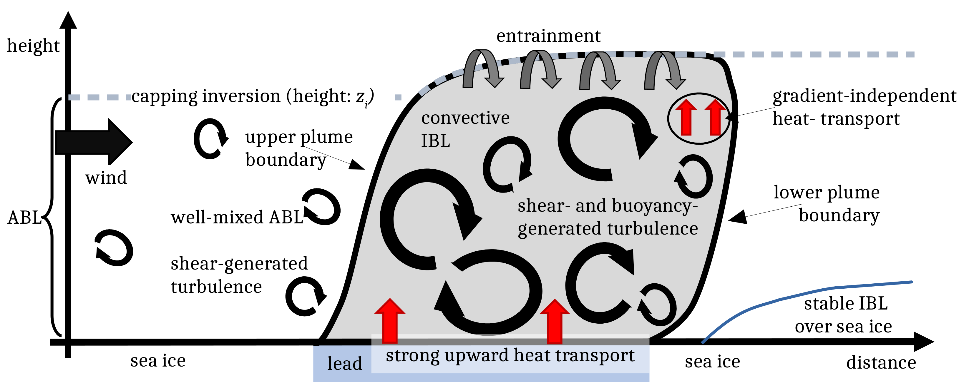
In the polar sea ice regions, the magnitude of transport mechanisms across the surface–atmosphere interface and, thus, the near-surface energy budget are strongly related to the characteristics of the surface, such as sea ice concentration, sea ice thickness, and surface temperatures. Both the surface characteristics and the corresponding interaction processes show high spatial and temporal variabilities. For example, between late autumn and early spring, with low incoming solar radiation, a thick sea ice surface acts as a good insulator between the relatively cold atmosphere and the warm ocean. Strong upward transports of heat and moisture are then almost limited to regions with polynyas or leads, where the latter represent elongated channels in sea ice. Both leads and polynyas are either free of ice or are covered with thin ice only. Thus, in this season, their surface is up to 40 K warmer than the air as long as no new ice has developed. This causes strong convection (convective plumes) and increased turbulent motion in convective internal boundary layers (IBL). They develop inside the atmospheric boundary layer (ABL) over the horizontally inhomogeneous environment of the leads (see Figure 1).

Leads, which are formed by divergent sea ice drift, are typically meters to a few kilometers wide and up to hundreds of kilometers long [4]. Locally, lead-generated convection can considerably alter wind, temperature, and also moisture fields within the shallow ABL over sea ice. For an almost lead-perpendicular flow in springtime conditions, Tetzlaff et al. [3] found based on airborne measurements during the Springtime Atmospheric Boundary Layer Experiment (STABLE) that a low-level jet can form upwind of leads. Further downwind, the low-level jet was then destroyed by lead-generated convection. They also found that the convective plumes can penetrate into the temperature inversion at the top of the ABL causing vertical entrainment, which amounted to 30% of the upward heat fluxes at the leads’ surfaces. The observations also pointed to regions of gradient-independent or counter-gradient heat transport in the plumes, as already stated by Lüpkes et al. [5] based on large eddy simulation (LES) and microscale model results. Concerning this feature, the nature of inhomogeneous convection over leads is similar to the nature of horizontally homogeneous convection (see the formulations by, for example, [6,7]). Entrainment, counter-gradient heat fluxes, and the enhanced heat transport over the lead surface in general contribute to the warming and to a stabilization of the downwind ABL including the formation of a stable IBL over the downwind sea ice surface (e.g., [2,3,8]). Potential sensitivities of such local ABL modifications on the meteorological forcing or on the lead geometry were investigated in numerous studies mostly using LES, microscale modeling, or both, e.g., [5,9,10,11,12].

Several atmospheric effects by leads—not only on a local scale, but also on a more regional scale—have been reported on in the literature. For example, this concerns effects on the balance of up- and downward heat fluxes [13,14], ABL temperature [15,16], stability over sea ice [15,17,18], near-surface relative humidity [19], or clouds [20,21]. Regarding ABL warming/cooling, the effects by leads are most pronounced for weak wind in clear-sky conditions during polar night [15,18,22]. Moreover, not only the actual open water percentage in sea ice may modify the ABL characteristics but also the distribution of sea ice and open water and, thus, the configuration of leads in sea ice. For example, Grötzner et al. [23] found by general circulation model simulations that there is a clear linkage between the transports at the atmosphere–ocean interface in the Arctic and the subgrid-scale distribution of sea ice. Such a dependence on sea ice distribution also holds for the ABL circulation over sea ice as Wenta and Herman [24] showed with a mesoscale model. Batrak and Müller [25] found a strong non-local effect on atmospheric conditions 500–1000 km away from the sea ice edge in a mesoscale model simulation considering an observed distribution of leads as compared to a simulation without these small-scale structures, while keeping the average large-scale sea ice concentration constant in both simulations. Recently, Heinemann et al. [26] obtained a good representation of near-surface in situ observations with a regional climate model by introducing new parameterizations, including one for the sea ice thickness to better reproduce thin ice often covering leads in winter. These studies clearly show that large-scale models, which cannot explicitly resolve leads and the atmospheric effects by lead-generated convection, can be strongly improved by somehow considering these subgrid-scale features.

Regarding the realistic reproduction of at least kilometer-wide leads in large-scale coupled ocean–sea ice models, for example, Wang et al., Hutter et al., and Zhang [27,28,29] obtained promising results by strongly increased resolutions of their respective sea ice models. However, as all studies pointed out, atmospheric interaction with the lead formation needs to be investigated in more detail. It is, however, unclear, up until now, if large-scale atmosphere models need specific parameterizations of the subgrid-scale lead-generated convection and related ABL processes. To better understand this, it is important to model the lead impact on atmospheric processes in much detail.

Regarding lead-averaged fluxes at the surface, Alam and Curry [30] and Andreas and Cash [31] showed a linkage to the width of the leads, with the heat transport over narrow leads of less than a 100 m width being most effective. Both formulated lead-width-dependent parameterizations for the corresponding transfer coefficients. By considering the lead width dependence, the average heat fluxes over open water can increase by 55%, for an observed distribution of leads (see [32] domain size: 60 × 66 km${}^2$).

Michaelis et al. [8,12] considered leads with a width L larger than at least 500 m. They showed that, for such leads, L is an important parameter that affects the fluxes of heat and momentum in the entire turbulent ABL above and downwind of leads. With their approach, they obtained a good agreement of their model results with LES [12] and with the observations from STABLE [8]. Michaelis et al. [8,12] applied horizontal grid sizes ${\Delta }_x=\mathcal{O}\left({10}^2\right)$ m in their simulations so that the entire convective plumes but not the single turbulent eddies were resolved. Thus, compared to Andreas and Cash [31], Michaelis et al. [8,12] considered much wider leads (500 m to 10 km width). Michaelis et al. [12] developed a lead-width-dependent turbulence parameterization, which was based on a non-local approach to account for the above-mentioned counter-gradient heat transport. It was also based on the approach by Lüpkes et al. [5], who formulated their parameterization for a lead of fixed width (1 km). Michaelis et al. [12] showed that their approach is robust against variations of the wind speed upwind of leads and of the surface temperature. Their approach was also applicable when the upwind stability and the ABL height were varied [8,33]. Simulations, however, using a local closure showed drawbacks, especially regarding entrainment and downwind ABL stratification [12].

The small-scale simulations of Michaelis et al. [8,12] focused on the effects over individual leads. Their findings regarding the necessary degree of complexity of the turbulence parameterization to sufficiently represent the microscale features in their microscale model raised the question as to how complex a parameterization should be to sufficiently reproduce lead-generated effects in non-convection-resolving models (e.g., regional climate models). Considering a region covered by a few grid cells of such a model, several leads of different geometry (widths) might exist in the individual grid cells, and the lead configuration might even change from one grid cell to the next one. However, the relevance of such changes for the ABL structure was unclear, until now.

The main goal of our study is to point at potential implications for non-convection-resolving models, which neither resolve the numerous microscale effects on the ABL over leads nor the exact distribution of sea ice and open water/leads. As a consequence, the topographical description of a sea ice region with leads, as it is realized in climate models, represents a strong difference to the real sea ice/leads topography. With the present study, we investigated the physical consequences of the idealized and simplified treatment in climate models.

As a first step, we used a microscale model for simulations of the flow over different series of leads, where the model allowed a more realistic treatment than in climate models, although still idealized. We applied the same model as used by Michaelis et al. [8,12] for convection over individual leads with microscale resolution (horizontal grid size ${\Delta }_x=200$ m). Thus, unlike climate models accounting for leads only by a reduced grid-cell-averaged sea ice concentration, the microscale simulations can distinguish and resolve lead patterns that are subgrid-scale for climate models.

In simulations of five cases, we used the same model with the same grid and domain sizes and the same prescribed domain-averaged sea ice concentration. To keep the analysis as simple as possible, in four cases, the only variable topographical parameter was the lead width L and the distance between the leads was set constant in each scenario. However, for a lead width of $L=5$ km, we selected a fifth case that differed by the distance between the leads from the main counterpart. Related simulations of this additional case aim to prove that topographical parameters other than the lead width are also important. Its impact needs a more detailed investigation in the future.

In the second step, we performed model runs of a sixth case, now with a coarse grid size of ${\Delta }_x=35$ km, which is comparable with the grid size of a regional climate model. Thus, leads were accounted for as in climate models, namely just by a sea ice concentration smaller than 100%, but with no other information on sea ice topography. However, the comparability of related simulation results to the lead-resolving simulations is ensured since the fractional sea ice concentration and domain-averaged surface temperature in the coarse-resolution simulations match the domain-averaged values of sea ice concentration and surface temperature of the microscale ones. This comparison finally allowed us to relate potential differences in domain-averaged quantities directly to the configuration of sea ice and open water. Moreover, we saved much computational time compared to LES by using a non-eddy-resolving model, whose turbulence parameterization has been developed for the flow over leads based on validations using LES and airborne observations; see [1,8,12]. We compare the ABL effects caused by the different configurations both qualitatively and quantitatively. This will underline the importance of leads and of their geometry for future parameterizations of the subgrid-scale atmospheric effects over lead-dominated sea ice regions in regional climate models.

Besides pointing at potential implications for non-convection-resolving models, our goal is to quantify differences in the model simulations regarding the applied turbulence parameterization. We considered both local and non-local approaches. Our study basically follows Michaelis [1], but we considered additional simulations and present more detailed analyses and discussions of the results. Lüpkes et al. [34] used a similar approach, but with preliminary versions of the parameterizations.

2. Model Description

Our modeling approach is as follows. A non-eddy-, but plume-resolving microscale model was used for idealized simulations of the convection over different lead configurations. We followed Michaelis et al. [12], who used the same model for comparable simulations over individual leads. Their non-eddy-resolving model results were all validated using LES. Namely, they used LES to optimize the adjustable parameters in their lead-width-dependent, non-local closure, which was also used in our study for most of the simulations (see Section 2.3.3). With that closure, they achieved a good agreement with LES, especially concerning heat flux patterns, plume inclinations, and downstream stratification for lead widths in the range 500 m $<L<$ 10 km and for different meteorological forcing. For example, a local maximum in the heat flux distribution in the convective plumes and the regions with gradient and gradient-independent heat transport were well reproduced. A good agreement with the LES was also shown for the wind field with a diminishing low-level jet over the lead, and for the structure of the momentum transport in the convective region. A similar validation using LES was performed by Michaelis [1] for domain-averaged profiles of the flow over two consecutive leads using the same initial conditions as in Michaelis et al. [12]. Finally, the same modeling approach was used by Michaelis et al. [8] to simulate three cases of lead-generated convection observed by aircraft during the campaign STABLE. They showed that the model is also capable of reproducing observed entrainment transport and variations near the top of the ABL, and that it can be applied to more stable inflow conditions and shallower ABLs than those considered by Michaelis et al. [12]. Thus, it was already proven that the modeling approach we used here is a good approximation of a much higher resolved but more expensive LES modeling, and of airborne observations of lead-generated convection. Hence, we consider this approach as reasonable, although the remaining differences to LES and the observations addressed by Michaelis et al. [8,12] should be investigated and confirmed in future studies.

2.1. Domain Characteristics

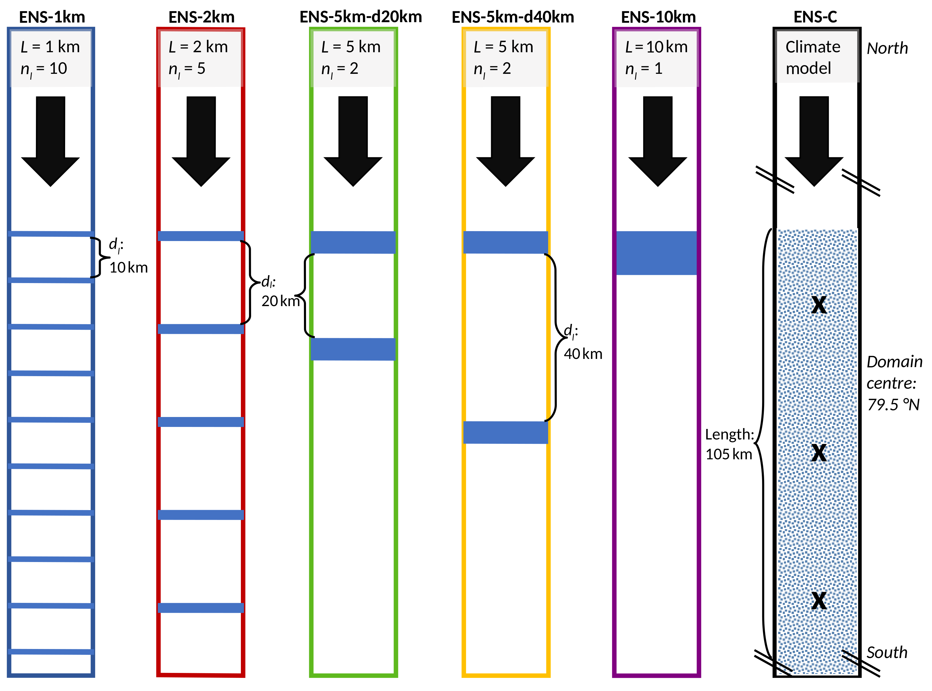
As shown in Figure 2, we distinguish six different cases. All cases are considered as representative for the quasi-2D flow over different configurations of sea ice and open water (leads) downwind of an inflow region over closed sea ice. For the inflow region, we prescribed a neutrally stratified ABL capped by a strong temperature inversion starting at height $z_i=300$ m and with an ABL-averaged flow velocity of approximately 5 ms${}^{-1}$. These inflow conditions represent one of the idealized cases of the ABL flow over individual leads considered by Michaelis et al. [12]. Note that all initial conditions used in their cases were selected according to atmospheric observations during several Arctic campaigns. All model domains have the same size (105 km length) and the same domain-averaged sea ice concentration (approximately 91%).

In five cases, we prescribed different ensembles of leads on a microscale grid with ${\Delta }_x=200$ m horizontal grid spacing. They differed by the lead width ($L=\{1,2,5,10\}$ km) and by the distance between the leads $d_l$ (cases ENS-1km, ENS-2km, ENS-5km-d20km, ENS-5km-d40km, ENS-10km, see Figure 2). Since we focused on possible atmospheric effects by varying L, the upwind edges of the leads closest to the inflow boundary were all at the same position in the corresponding domains. This guarantees that, in all model runs, the inflow profiles are the same at the upwind boundary of the first lead. The surface temperatures of the leads were prescribed to 270 K (representing leads covered by thin, new ice). Between the leads, we assumed 100% thick sea ice cover with a surface temperature of 250 K.

The sixth case should represent a few grid cells of a regional climate model, wherein leads were not explicitly resolved so that the surface topography differed strongly from the other cases. It is abbreviated by ENS-C (Figure 2), where ’C’ hints to climate models. The model domain of case ENS-C is arranged using a grid with ${\Delta }_x=35$ km horizontal grid spacing. As mentioned in Section 1, the corresponding sea ice concentration in each grid cell is the same as the domain-averaged sea ice concentration in the other five cases. This leads to the same domain-averaged surface temperature (approximately 251.9 K). Thus, although the topography in case ENS-C differs completely from the other cases, a comparison of domain-averaged quantities is still possible [1,34]. This setup allowed us to derive potential implications for regional climate models wherein leads and the related ABL effects are not resolved.

For all model domains, we prescribed the momentum roughness lengths as $z_{0,i}={10}^{-3}$ m and $z_{0,w}={10}^{-4}$ m for sea ice and open water surfaces, respectively. The ratio between the surface roughness lengths for heat and momentum is assumed as 1/10.

2.2. Applied Model

All our simulations were performed with the microscale, 2D, non-hydrostatic atmosphere model METRAS (MEsoscale TRAnsport and Stream model, [35,36], dry version). The model’s equation system consists of the Boussinesq-approximated primitive equations, which are solved on a staggered Arakawa-C grid. Basically, we followed the setup used by Michaelis et al. [8,12] and Michaelis [1] for their simulations over individual leads. Hence, we also prescribed fixed values at the inflow boundary and a gradient-zero approach at the outflow boundary for the temperature. For the wind components, the same boundary conditions were used at in- and outflow (zero-gradient for boundary-parallel components and a direct calculation of boundary-normal components). We refer to the model’s documentation for a more detailed explanation of the boundary conditions; see [36]. Similar to previous studies [1,8,12], we applied a vertical grid spacing of ${\Delta }_z=20$ m in the ABL of height $z_i=300$ m and a more stretched grid up to the model’s top at about 9000 m. In all our simulations, turbulence was treated as a subgrid-scale and, thus, a completely unresolved process requiring parameterization. We used different parameterizations for the turbulent heat and momentum fluxes (see Section 2.3).

2.3. Turbulence Parameterizations

We distinguished between parameterizations used for simulations of case ENS-C with fractional sea ice cover in each surface grid cell and for the lead-resolving simulations.

2.3.1. Surface Fluxes

In the surface layer, which was represented by the first grid cell above the surface, we basically applied the Monin–Obukhov similarity theory in all model runs using Businger–Dyer functions [37,38]. For simulations of case ENS-C, which did not resolve the plumes over individual leads, we then calculated the turbulent fluxes in each surface grid cell with a flux-averaging method following the blending height concept [39]. For the lead-resolving cases, the flux-averaging method was not necessary since each surface grid cell consisted of either 100% thick sea ice or open water.

2.3.2. Closures Used for Case ENS-C

For the parameterization of the mixed layer turbulent fluxes, we applied different first-order closures, a local mixing-length scheme and various non-local schemes. We applied two versions of a non-local closure for model runs of case ENS-C, as well as two other versions, described in Section 2.3.3, for the runs resolving lead-generated convection. Thus, each lead scenario was simulated with three different closures so that the differences related to the used closures could be analyzed.

In all simulations of case ENS-C, we basically used the local mixing-length closure of Herbert and Kramm [40] in regions with stable stratification. In one simulation of this case, this closure was also used for neutral and unstable stratification developing over the fractional sea ice cover. However, it is well known that local mixing-length closures cause drawbacks, especially in strongly convective regimes (e.g., [6,7,41,42]), since gradient-independent or counter-gradient fluxes cannot be reproduced and the potential temperature cannot show the well-documented slight increase with height often observed in the upper half of the convective ABL.

Thus, in the other two simulations considered for case ENS-C, we applied a non-local closure with a gradient-correction term to account for the counter-gradient transport. We used the closure by Lüpkes and Schlünzen [41], who originally derived their parameterization for turbulent fluxes in a strongly convective ABL associated with Arctic cold-air outbreaks, where they obtained a good agreement with airborne measurements. In this closure, non-local effects were accounted for by also relating the turbulent fluxes to the ABL height $z_i$ and to the surface buoyancy flux over the horizontally homogeneous surface. Moreover, the cold-air outbreaks studied by Lüpkes and Schlünzen [41] were associated with a strong growth of $z_i$ with increasing distance to the ice edge by convection penetrating into the inversion layer. This caused negative heat transport at the ABL top (vertical entrainment). Unlike these conditions, for case ENS-C, we could expect much weaker convection due to the high sea ice concentration of 91%. This led to low average surface temperatures in the grid cells with fractional sea ice cover, causing only a small upward heat transport into the ABL. Hence, the penetrating convection was probably much smaller than in the cases studied by Lüpkes and Schlünzen [41]. Therefore, we applied their non-local closure in two versions. In the first version, we assumed a constant mixed layer height $z_i$. In the second version, we applied a method for the $z_i$-determination as described in Section 2.3.4.

2.3.3. Closures Used for the Lead-Resolving Cases

For the simulations of the cases with explicitly resolved leads, we used the following three parameterizations. First, we again used the mixing-length closure of Herbert and Kramm [40] and, thus, the same as in one model run of case ENS-C. The two other parameterizations were based on a non-local closure that was derived by Michaelis et al. [12] for convection over leads of different widths. Their approach was based on Lüpkes et al. [5], who showed that the parameterization of the turbulent heat fluxes over individual leads should include the distance to the lead to account for the horizontal inhomogeneity of lead-generated convection. This closure differs from traditional non-local closures, since those were derived for homogeneous terrain, but not for inhomogeneous surfaces, as those considered in the lead-resolving cases. The latter kind of inhomogeneity is explicitly taken into account by the non-local closure of Michaelis et al. [12]. Hence, while inside the convective plumes over leads, a non-local closure was used, a local closure was used outside. The transition is determined by the positions of the upper and lower plume boundaries (see also Figure 1). Michaelis et al. [12] improved their results concerning the decaying convection downwind of the leads by including the lead width L in the decay function they used.

Here, we used two versions of the closure, which differed by the treatment of $z_i$. In the most simple one, the growth of the upper plume boundary was limited by the upwind ABL height $z_i$, for which Michaelis et al. [12] prescribed a fixed value of 300 m in their simulations. This was in agreement with the observed vertical profile of the potential temperature used in the inflow region. In the second version, $z_i$ varied with distance from the leads. The method for its determination is described in the following subsection.

2.3.4. Treatment of the ABL Height in Simulations with the Non-Local Closures

For both the lead-resolving cases (ENS-1km–ENS-10km) and case ENS-C, we expect that convection will cause mixing in the entire ABL. This includes convection penetrating into the inversion and, thus, to higher altitudes than to its bottom prescribed at $z_i=300$ m in the inflow region causing vertical entrainment. In cold-air outbreaks, $z_i$ increases strongly to values of more than 1 km after the air mass has reached the open ocean with a surface temperature near the freezing point [41]. Over sea ice with leads, this increase is, however, only small due to the short fetches over leads and, thus, a much weaker domain-averaged convection. However, although limited to small areas, penetrating convection was, for example, shown in the observations during STABLE [3]. The observed entrainment fluxes amounted to up to 30% of the surface heat fluxes over the leads, which led to different values for $z_i$ on the upwind and downwind side of the leads [3]. Thus, Michaelis et al. [8] showed that with METRAS simulations of the cases from STABLE, an improved agreement with the observations can be obtained regarding the increase of $z_i$ and the related entrainment when the closure by Michaelis et al. [12], assuming constant $z_i$, is modified by considering variations of $z_i$ in the flow direction.

Lüpkes and Schlünzen [41] and Michaelis et al. [8] used different approaches to calculate $z_i$ in their studies. While the former related $z_i$ to the vertical position of the minimum heat flux at each horizontal grid point, the latter determined $z_i$ by tracking the vertical position of a specific contour line of the potential temperature in the inversion layer. Both methods, as well as other commonly used methods to diagnostically determine $z_i$, are explained in more detail by Sullivan et al. [43]. To evaluate potential advantages regarding the representation of $z_i$-variability and related entrainment, we used the non-local closures either with constant $z_i$ or with variable $z_i$ by applying the method of Michaelis et al. [8] to diagnostically calculate $z_i$ (see also Figure S1 in the Supplementary Material).

In total, we considered three simulations for each case summarized in

Table 1. Overview of the model runs and the corresponding turbulence closures used in this study for the lead-resolving cases (ENS-1km, ENS-2km, ENS-5km-d20km, ENS-5km-d40km, and ENS-10km) and for the case ENS-C with the same fractional sea ice concentration in each grid cell (see Figure 2 for the cases).

	Model Runs
Cases	MIX [40]	NL-M20 [12]	NL-LS96 [41]	NL-M20-zi	NL-LS96-zi
Lead-resolving	Local mixing-length closure	Non-local closure for lead-generated plumes, lead-width-dependent, constant $z_i$	-	Non-local closure for lead-generated plumes, lead-width-dependent, variable $z_i$	-
ENS-C	Local mixing-length closure	-	Non-local closure for convection over homogeneous surfaces, constant $z_i$	-	Non-local closure for convection over homogeneous surfaces, variable $z_i$

. Simulations using only the mixing-length closure are henceforth abbreviated by MIX. Simulations with the above-mentioned non-local closures using constant $z_i$ are henceforth abbreviated by NL-LS96 for case ENS-C and by NL-M20 for the lead-resolving cases. Simulations with the same non-local closures, in which we allow variations of $z_i$, are henceforth abbreviated by NL-LS96-zi and NL-M20-zi, respectively.

2.3.5. Mixed-Layer Momentum Fluxes and Linkage with the Surface Layer

For the simulations using the non-local closures for the heat fluxes, the subgrid-scale momentum fluxes are calculated prescribing the eddy diffusivity for momentum as a function of the eddy diffusivity for heat (see [36,41]). Moreover, in all closures used, a continuity of the fluxes at the top of the surface layer is ensured.

3. Results

This section is divided into two parts. First, we present simulated vertical cross-sections of mean atmospheric quantities as well as the horizontal evolution of the turbulent fluxes with increasing distance to the inflow region for two different layers of the ABL, for all cases. Second, we show domain-averaged vertical profiles of both mean atmospheric quantities and turbulent fluxes to point at the differences in the ABL structures caused by the different lead patterns and different parameterizations. All corresponding figures show model results obtained after quasi-stationary conditions were reached.

3.1. Individual ABL Patterns

Figure 3 shows vertical cross-sections of potential temperature and wind speed obtained with the METRAS simulations NL-M20-zi for the cases with explicitly resolved leads and NL-LS96-zi for case ENS-C. Potential temperatures are shown as deviations from the inflow potential temperature of 250 K and wind speeds as dimensionless values normalized by the ABL-averaged inflow wind speed of 5 ms${}^{-1}$. Based on the results of previous studies mentioned in Section 2, we consider these simulations as the most appropriate applications to reproduce either ABL structures over resolved series of leads by a non-eddy-resolving model, or ABL structures over the homogeneously heated surface of case ENS-C by a non-convection-resolving model.

As expected, a warming of the ABL is obtained by all simulations with increasing distance to the inflow region (Figure 3a,c,e,g,i,k). However, the mean ABL potential temperature increase with distance slightly differs among the different cases. Moreover, the whole ABL structure and, thus, stratification considerably differ between case ENS-C and the other cases. For case ENS-C, a slightly unstable layer is obtained in the lowermost 100 m, followed by a neutrally stratified layer up to approximately 250 m height, and slightly stable stratification between 250 m height and $z_i$ over the entire domain (Figure 3k). In the lead-resolving simulations, an inclined unstable layer is simulated over the leads resembling the convective IBLs. Further downwind over sea ice, stable IBLs are shown in the lowermost 100 m, and a much weaker (but still stable) stratification exists between 100 m height and the ABL top (Figure 3a,c,e,g,i). The stability of the downwind IBL increases from case to case with increasing lead number. For the cases with $L\ge 5$ km, weak gravity waves were simulated in the strengthening stable IBL close to the outflow edge of the domains (Figure 3e,g,i).

The ABL patterns of the horizontal wind speed also strongly differ between the microscale and the coarser-resolved simulations (Figure 3b,d,f,h,j,l). For the lead-resolving cases, pronounced wind speed maxima are simulated upwind of the leads. Especially near the leads closest to the inflow boundary, these maxima occur slightly below the capping inversion and the flow velocity exceeds the ABL-averaged inflow velocity by approximately 15–20%. Over the leads, the maxima vanish by the lead-generated convection. This pattern is repeatedly shown over each lead in the cases with more than one lead. Moreover, the strongly stable IBL over sea ice in the cases with $L\ge 5$ km leads to strong local wind speed minima over sea ice. A weak local wind speed maximum is also obtained for the case ENS-C, but this one exceeds the mean ABL flow speed by less than 10% (Figure 3l). Further downwind, the wind field only marginally differs from the upwind ABL flow.

In Figure 4 and Figure 5, we show the horizontal development of turbulent heat and momentum fluxes near the surface and near the ABL top as obtained with the simulations NL-M20-zi and NL-LS96-zi. In the lead-resolving simulations, the sensible heat fluxes show maxima of up to 190 Wm${}^{-2}$ close to the lead surfaces and slightly negative values downwind over sea ice (Figure 4a). For case ENS-C, the grid-cell-averaged heat flux is at approximately 10–20 Wm${}^{-2}$ in every grid cell.

Due to vertical wind shear in the inflow region, the momentum fluxes at 10 m height amount to about 0.04 Nm${}^{-2}$ upwind of the respective domains (Figure 4b). Further downwind, we obtain momentum fluxes of up to 0.07 Nm${}^{-2}$ in the lead-resolving simulations. Moreover, the small-scale structure of the momentum fluxes differs from case to case. While for the cases ENS-1km and ENS-2km the highest fluxes are obtained close to the downwind lead edges, these maxima occur already in the first half of the leads in the cases with $L\ge 5$ km. For these cases, we obtain a slightly inhomogeneous development of the near-surface fluxes in the second half of the domains, which probably resembles the influence of the above-mentioned weak gravity waves. For case ENS-C, we obtain only slightly increased values of about 0.05 Nm${}^{-2}$ in each grid cell.

Near the ABL’s top, for most lead-resolving cases, strongly negative heat fluxes are simulated (Figure 5a). This denotes vertical entrainment above and downwind of the leads. The entrainment heat fluxes amount to about 20% of the near-surface fluxes. The highest entrainment is obtained over the leads closest to the inflow boundary. The reason is that there the plumes are strongest because the difference between the temperatures of the inflow air and the lead is highest. In addition, the stratification upwind of these leads is neutral, whereas it is slightly stable upwind of the leads further downwind. The latter causes a weakening of the plumes and, thus, also of entrainment. For case ENS-C, the heat fluxes at 300 m height are slightly below 0 Wm${}^{-2}$ in each grid cell. For the momentum fluxes at 300 m, we obtain values close to zero in both lead-resolving and non-lead-resolving simulations (Figure 5b).

In the supplementary material (Figures S2–S7), we show the results of the quantities discussed in this section as obtained with the other model runs (MIX, NL-M20, and NL-LS96).

3.2. Domain-Averaged Vertical Profiles

As shown in Figure 3, Figure 4 and Figure 5, we obtain various small-scale ABL structures above and downwind of the leads in the convection-resolving simulations. Apparently, the characteristics of such structures depend on the lead width [12]. Such horizontal inhomogeneity is especially important when it also affects the domain-averaged values. This would be relevant mainly for the case ENS-C, for which such structures cannot be resolved. Therefore, in Figure 6 and Figure 7, we show domain-averaged ABL profiles of the sensible heat flux, potential temperature, horizontal wind speed, and the momentum flux. Moreover, to point at potential differences among the different parameterizations applied in this study, results of all 18 simulations are shown.

Basically, the ABL effects by the leads and by the lead geometry are clearly obvious in the domain-averaged vertical profiles, irrespective of the parameterization (Figure 6 and Figure 7). For example, we obtain surface heat fluxes of about 11–12 Wm${}^{-2}$ for case ENS-C, which is lower than for all lead cases (Figure 6a–c). There, the surface heat fluxes are at approximately 12.5 Wm${}^{-2}$ for case ENS-1km, and they increase with increasing lead width to 16 Wm${}^{-2}$ for case ENS-10km. Thus, the domain-averaged surface heat fluxes obtained for case ENS-C are up to 30% lower than for the lead-resolving simulations. The range of surface heat fluxes in the lead-resolving simulations is smallest for the model runs MIX (Figure 6a) and largest for the model runs NL-M20-zi (Figure 6c) and, thus, for the simulations using the best representation of the small-scale turbulence as compared to observations and LES (see [1,8,12]). This indicates a clear relationship between the lead width and the average surface heat transport.

We obtained different results depending on the case, not only for the surface fluxes, but also for the entire heat flux profile. In particular, for the heat flux minima near the inversion layer, the parameterization plays a role. In the model runs using the non-local closures, we obtain downward heat fluxes near the inversion indicating entrainment, whereas no entrainment is simulated in the model runs MIX at all (Figure 6a–c). The largest entrainment is obtained by simulations using the method with varying $z_i$ (model runs NL-M20-zi and NL-LS96-zi), which agrees with the model results obtained by Michaelis et al. [8] for observed convection over individual leads. Moreover, the smaller the lead width, the larger are the domain-averaged entrainment fluxes. However, the domain-averaged entrainment fluxes for the cases with narrow leads ($L\approx 1$ km) might be too strong in the runs NL-M20-zi as discussed by Michaelis [1] using a comparison to LES. For case ENS-C, we obtain vertical entrainment only by the run NL-LS96-zi with a similar value as shown for the lead-resolving cases with $L\le 2$ km (Figure 6c).

Three main effects by leads can be derived from the domain-averaged potential temperature profiles. First, a strongly stably stratified ABL on average is shown in all lead-resolving model runs in the lowermost 100 m, irrespective of the lead configuration and strongest for the cases with $L\ge 5$ km (Figure 6d–f). The stabilization effect by leads over sea ice was shown also in other studies, e.g., [18]. On the contrary, an unstably stratified ABL is simulated for case ENS-C. Second, the domain-averaged warming of the ABL center is smallest for the cases with $L\le 2$ km and largest for case ENS-10km. Both the stable IBL and the ABL warming are strongest in the simulations NL-M20-zi and weakest in the simulation MIX. This indicates that gradient-independent heat transport and vertical entrainment both enhance the warming effect. Third, only a small quantitative difference is shown between the potential temperature profiles obtained for the cases ENS-1km, ENS-2km, and ENS-C. However, differences in the simulated ABL stabilities are fundamental, especially in the simulations using non-local closures.

The domain-averaged vertical profiles of the horizontal wind speed also show three main features (Figure 7a–c). First, the lowest wind speeds are obtained for the lead-resolving cases with $L\ge 5$ km, which most probably resembles the influence of the stable IBL (see Figure 6d–f). Second, a local wind maximum is shown for all cases close to the ABL top, where it is highest for case ENS-2km. Third, the variability of the results among the different cases is much larger in the simulations MIX than in those using a non-local closure. For the momentum fluxes, such a difference in the variability of the results is not that high (Figure 7d–f). Here, the main result is a nearly linear vertical profile for case ENS-C, whereas we obtain non-linear vertical profiles for the lead-resolving cases. This fundamental difference is especially shown in the simulations using the non-local closures. In addition, the surface momentum fluxes show large differences between approximately 0.05 Nm${}^{-2}$ for case ENS-C and approximately 0.025–0.03 Nm${}^{-2}$ for case ENS-10km.

For both mean quantities and turbulent fluxes, some of the domain-averaged ABL profiles strongly depend on the configuration of leads, but especially on the lead width. The wider the leads are, the larger the differences between the lead cases and case ENS-C.

4. Discussion and Conclusions

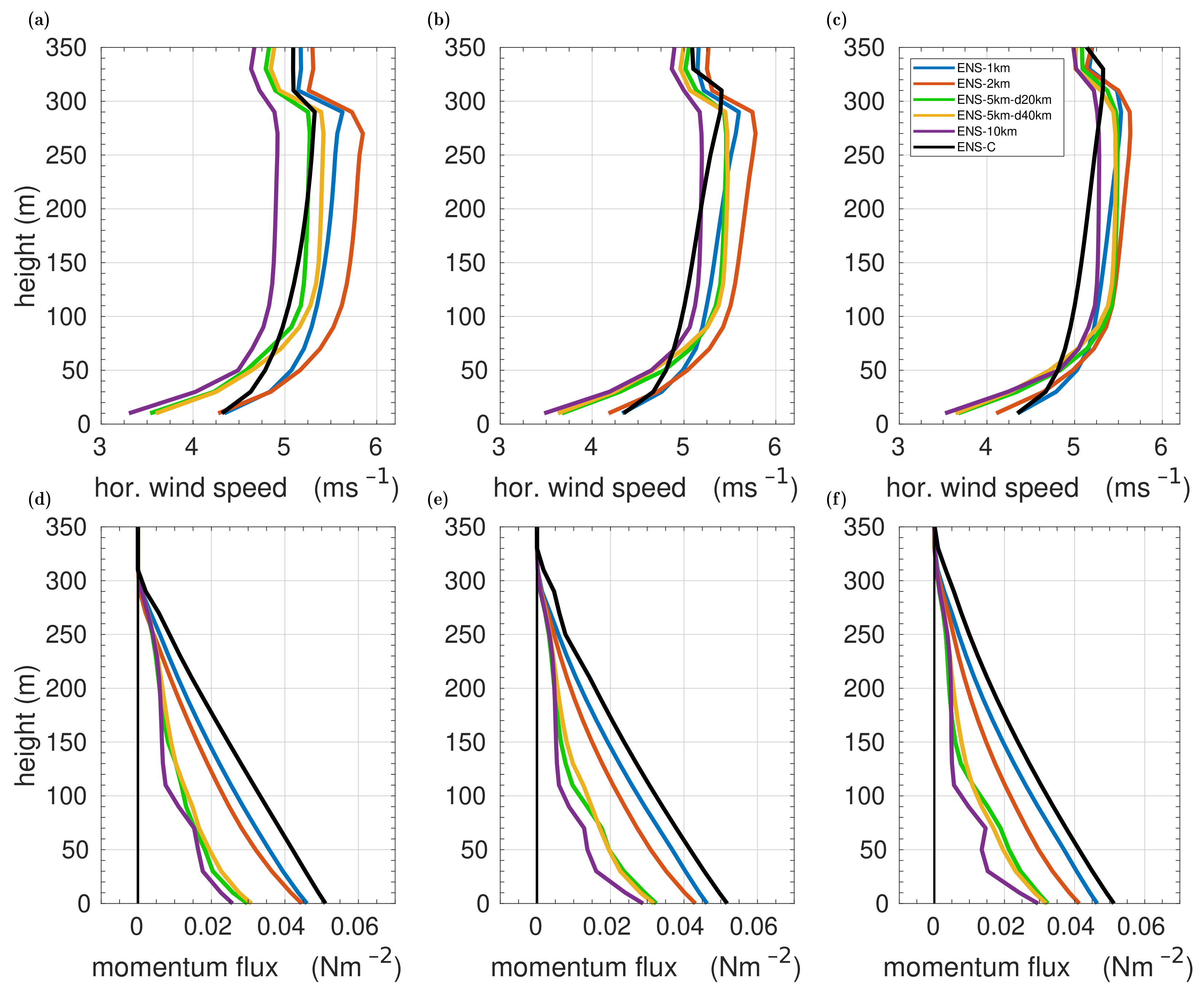
Our results show that the actual configuration of leads in a sea ice covered region has a clear influence on ABL characteristics, which was obvious in the respective ABL structures over the individual domains, as well as in the domain-averaged vertical profiles of wind, temperature, and turbulent fluxes. Moreover, as already indicated by Michaelis [1] and Lüpkes et al. [34], the geometry (widths) of the leads also influence these averaged results. Hence, the domain-averaged ABL structures depend, to a certain degree, on the lead width, which shows the importance of this quantity.

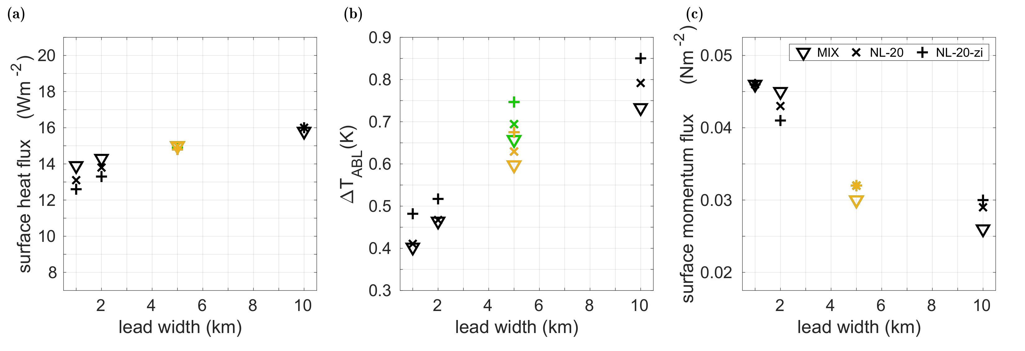
The domain-averaged vertical profiles show that certain characteristic quantities, for example, the average turbulent fluxes at the surface or the average warming of the ABL, either increase or decrease monotonically with increasing lead width. To highlight this rather qualitative result also quantitatively, and to point at possible functional dependencies, we show the fluxes and ABL warming in Figure 8 as a function of lead width obtained from all simulations for the lead-resolving cases.

Apparently, the domain-averaged surface sensible heat fluxes show a nearly linear dependence of the lead width, while both momentum fluxes and ABL warming show a non-linear dependence (Figure 8). This non-linearity depends only slightly on the closure. However, the relation between heat fluxes and the lead width deviates slightly from linearity when the non-local closure with variable $z_i$ is used (Figure 8a). Moreover, it is remarkable that although the sensible heat flux increases only slightly with lead width, the ABL warming increases by a factor of about 1.8 when the lead width increases from 1 km to 10 km. This can be explained by the positions of the leads within the respective domains. One can speculate that if the 10 km-wide lead of the case ENS-10km was located much closer to the outflow edge, the domain-averaged ABL warming would be much lower. This indicates that the actual position of the leads within the domain is important to be considered at least for lead-perpendicular inflow conditions. 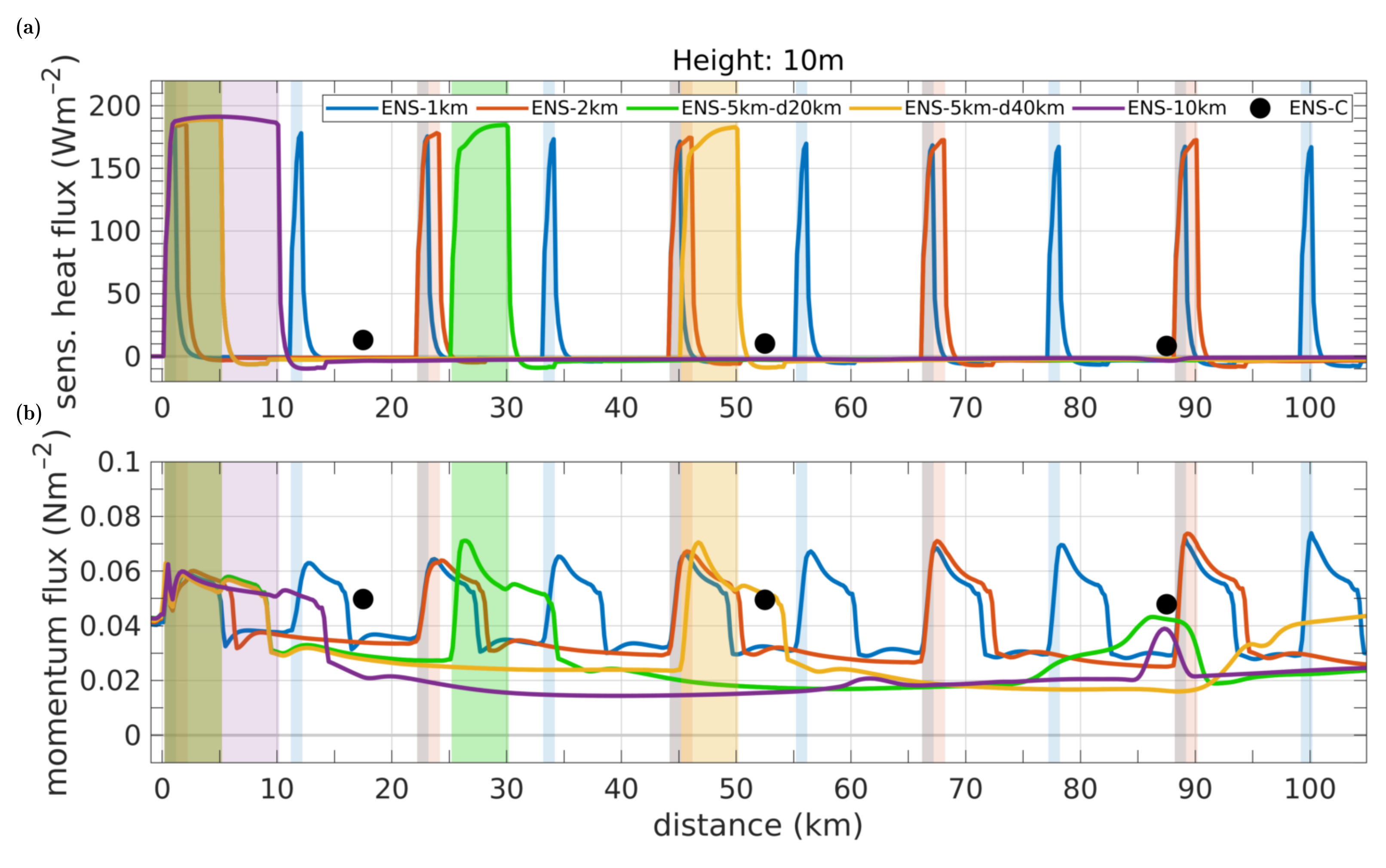The effect on the domain-averaged ABL warming is also visible by the differences between the two cases with the same lead width but different distances between the leads (ENS-5km-d20km and ENS-5km-d40km, Figure 8b). However, the effect is not large in this case. Moreover, the domain-averaged heat and momentum fluxes show almost no differences when the distance between the 5 km-wide leads is varied, and variations in the lead width have a much larger effect on the flux profiles (Figure 6 and Figure 7). Finally, we stress that the result concerning the sensible heat flux should not be mixed with the results of Andreas and Cash [31] for small leads of less than 100 m width (not considered here). Their results showed that the fluxes over the leads increased with decreasing width, but unlike in our study, they considered only the lead area and not the complete domain.

Our results suggest that besides the above-mentioned differences between the lead-resolving simulations, results of the latter differ also strongly from those of case ENS-C, and thus from results that a regional climate model would achieve with a grid spacing of 35 km if the same domain-averaged surface temperature would be predicted. The largest difference was shown between ENS-C and the model runs over leads with $L\ge 5$ km. To underline these differences also quantitatively, we show in

Table 2. Overview of the domain-averaged values of selected characteristic quantities obtained by the model runs NL-M20-zi for the lead-resolving cases ENS-1km, ENS-2km, ENS-5km-d20km, ENS-5km-d40km, and ENS-10km, and by the simulation NL-LS96-zi for case ENS-C. Cases and model runs are described in Figure 2 and Table 1 (see Section 2).

	Case
Quantity	ENS-1km	ENS-2km	ENS-5km-d20km	ENS-5km-d40km	ENS-10km	ENS-C
Surface heat flux (Wm${}^{-2}$)	12.6	13.3	14.9	14.8	16.0	10.9
Minimum heat flux in ABL (Wm${}^{-2}$)	−5.1	−4.1	−2.1	−2.2	−1.6	−4.2
ABL warming (K)	0.48	0.52	0.75	0.68	0.85	0.54
ABL stratification below 100 m (K(100 m)${}^{-1}$)	0.01	0.08	0.32	0.24	0.48	−0.06
ABL stratification (K(100 m)${}^{-1}$)	0.10	0.16	0.17	0.16	0.20	0.02
Minimum wind speed in ABL above 10 m (ms${}^{-1}$)	4.4	4.1	3.7	3.6	3.5	4.3
Maximum wind speed in ABL (ms${}^{-1}$)	5.5	5.6	5.5	5.5	5.3	5.3
Surface momentum flux (10${}^{-2}$Nm${}^{-2}$)	4.6	4.1	3.2	3.2	3.0	5.1

domain-averaged values for selected characteristic quantities as obtained by the simulations using non-local closures with varying $z_i$ (NL-M20-zi and NL-LS96-zi). Results from the other simulations are shown in Tables S1–S2 as supplementary material.

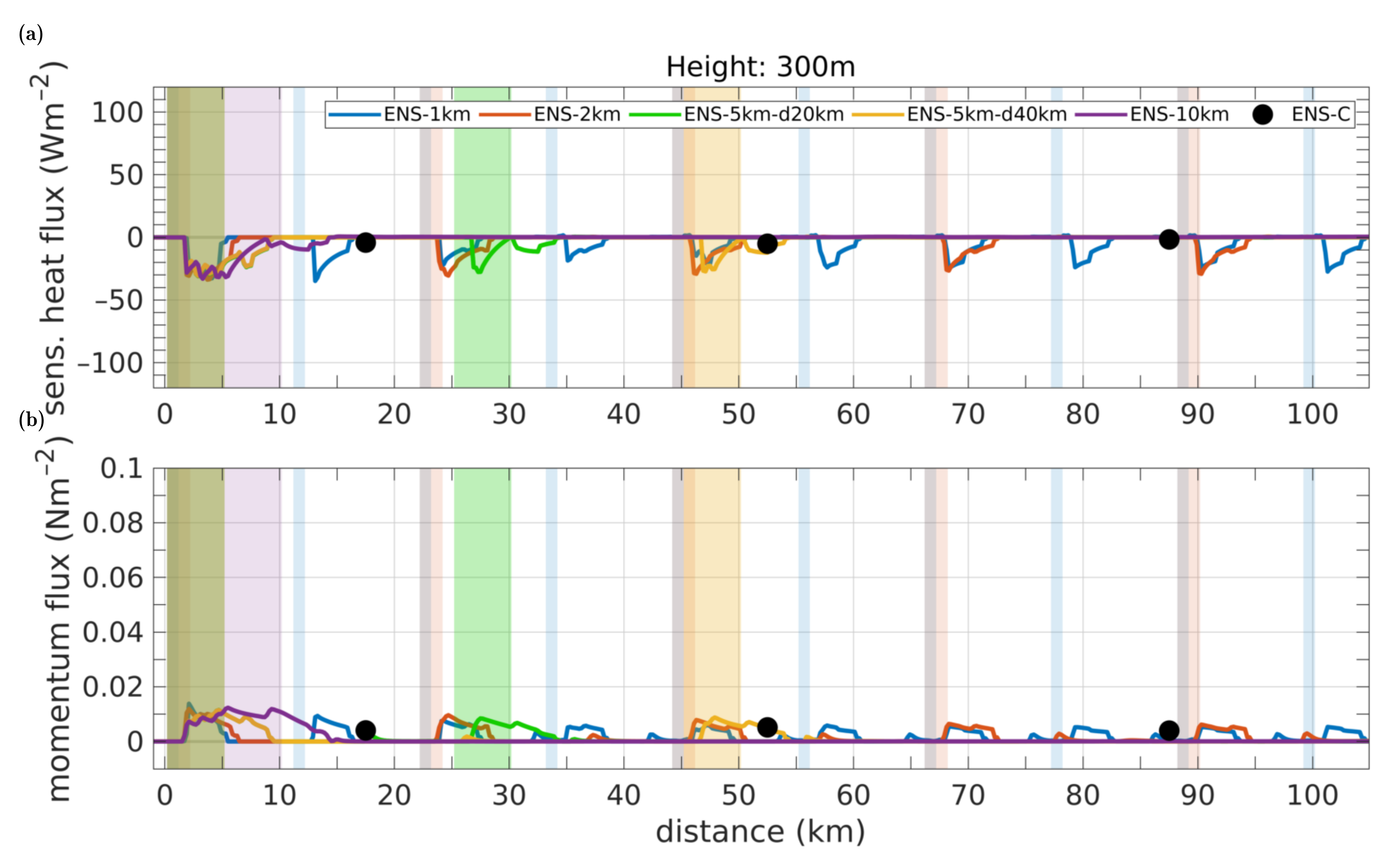
As Table 2 shows, differences between the lead-resolving cases and case ENS-C are largest for the surface turbulent fluxes as well as for the stability, especially in the lowest 100 m. Consequently, we can formulate at least three implications for models that cannot explicitly resolve leads. First, surface heat fluxes are slightly underestimated by such models. Second, surface momentum fluxes are slightly overestimated by them, and third, the stabilization effect by leads in the lowest 100 m of the ABL is completely missing. Thus, as already stressed by Michaelis [1], the nature of the domain-averaged heat transport in this layer is fundamentally different, depending on whether leads are explicitly resolved or not (gradient transport for case ENS-C, gradient-independent transport in the lead-resolving simulations). Another implication for case ENS-C concerns the inability to reproduce the non-linearity in the vertical momentum flux profile that was shown especially for the cases with $L\ge 5$ km (see Section 3).

Regarding the structures of the domain-averaged ABLs, we also found differences between the results obtained with different parameterizations (see Section 3, Table 2, and the Supplementary Material). The largest differences were obtained between the simulation using the local closure for case ENS-C (model run MIX) compared to the simulations with the non-local closure and a varying $z_i$ for the lead-resolving cases (model runs NL-M20-zi). Thus, counter-gradient transport and the entrainment had a large impact on the results. These differences to the runs of case ENS-C were slightly smaller when the local closure was replaced by a non-local closure (runs NL-LS96 and NL-LS96-zi). However, even with the simulation NL-LS96-zi, we still obtained fundamental differences between the lead-resolving cases and case ENS-C. Hence, although the non-local closure with variable $z_i$ improved the non-convection-resolving model results, with respect to the lead-resolving ones, large differences in the domain-averaged ABL profiles of both mean quantities and turbulent fluxes remain. All this points to a large relevance of the treatment of leads in climate models using grid sizes far beyond those needed to resolve lead-generated convection.

Our microscale simulations were carried out with an atmospheric model resolving plumes over leads but not the small-scale eddies. This was achieved with only little numerical effort as compared to LES resolving both plumes and eddies (roughly 1/1000 of the CPU time, [1,5]). Considering the results, we need to point at some methodological limitations. First of all, our runs were strongly idealized and limited to a certain set of forcing conditions. Further simulations with different meteorological forcing (wind, surface temperatures, ABL height) are necessary to confirm our above findings. Also, we stress that we compared model results with model results but did not consider observations, which are not available in the required resolution and domain size. However, the parameterizations we used have been validated against airborne observations and LES in previous studies for the flow over one lead [8,12] or over two consecutive leads [1]. The corresponding observations are available from one campaign only with the sufficient vertical and horizontal resolution (see [3]). Thus, in the future, data from similar campaigns would be beneficial. In addition, our study might stimulate similar sensitivity studies with LES, and also observed distributions of leads might be considered then like those addressed in Marcq and Weiss [32] and Tetzlaff [44].

In our model simulations, no elevation (freeboard) of the sea ice is considered. Thus, we do not account for the form drag of the floe edge as in Lüpkes et al. [45]. However, since we use two different roughness lengths for open water and sea ice surfaces, a purely mechanically induced IBL develops in the model when the flow crosses the lead surfaces. However, for the temperature difference of 20 K that we apply, the mechanically induced IBL plays only a negligible role with respect to the very strong thermally induced IBL. Moreover, sea ice pressure ridges (accounted for by the increased sea ice roughness length) would make a larger effect than the few edges of the leads due to the large distances to each other. This is different in a marginal sea ice zone with much smaller sea ice fraction and a much larger number of floe edges (see [45,46]). Nevertheless, there is certainly a step change in roughness between open water and sea ice. In future work, one could indeed investigate the effect of this step change in summer conditions when the stratification over leads is close to neutral. This would probably mainly affect the momentum budget.

We also stress that our model was not coupled with sea ice. This might have affected the stability at the downstream side of leads because the slightly heated plumes could not warm the sea ice surface. However, we expect that even in a coupled version, the stabilization of the ABL by leads would not disappear completely since it has already been described by coupled 1D models (see [15,18]). Additional runs similar to ours, but with coupled models, might be useful in the future to better understand air–ice interaction over sea ice with leads (see also [3,8]). Our results showed that the treatment of leads has a strong impact on the energy fluxes and thus also on the energy budget, which would finally also affect the sea ice surface temperature. In a coupled model, the small-scale wind field would furthermore affect the formation of leads, which would trigger several feedback mechanisms depending on the season. This might then affect the sea ice concentration, so that coupled small-scale modeling resolving leads and processes over leads could be beneficial also for ship navigation.

Our analysis is limited to cases of dry convection over leads since we neglected phase transitions of water. Such an assumption can be justified as shown by the observations during STABLE [3]. We considered newly refrozen rather than ice-free leads by prescribing the leads’ surface temperatures as 270 K. Over such leads, which are typical for low air temperatures, and which were observed mostly during STABLE, sensible heat fluxes clearly exceed the latent heat transport. The lead-generated convection can even cause ABL clouds to dissipate [20,21].

To summarize, we can formulate three main conclusions based on our results. First, the domain-averaged vertical profiles of wind, temperature, and turbulent fluxes strongly depend on the configuration of sea ice and open water (leads). Second, the geometry (width) of the lead plays an important role due to its clear influence on the domain-averaged results. Concerning this feature, our results indicate a non-linear functional relation between domain-averaged quantities (ABL-warming, momentum fluxes) and the lead width. Moreover, we hint at further topographical parameters that might have an impact on these results, such as the position of the leads within the domain and their distance to each other. Third, we stress the importance of gradient-independent turbulent transport and vertical entrainment for the parameterization in microscale, non-eddy-resolving models, as well as in non-convection-resolving models. Altogether, our results imply that the actual representation of leads and their distribution in a domain of a regional climate model can strongly influence atmospheric patterns in related simulations. These findings could help to promote the development of an improved parameterization for turbulent transport and convection in climate and numerical weather prediction simulations over lead-dominated sea ice regions.

References

1. Michaelis, J. Modelling and Parametrization of Turbulent Convective Processes over Leads in Sea Ice. Ph.D. Thesis, Universität Bremen, Bremen, Germany, 2020. [Google Scholar] [CrossRef]
2. Vihma, T.; Pirazzini, R.; Fer, I.; Renfrew, I.A.; Sedlar, J.; Tjernström, M.; Lüpkes, C.; Nygard, T.; Notz, D.; Weiss, J.; et al. Advances in understanding and parameterization of small-scale physical processes in the marine Arctic climate system: A review. Atmos. Chem. Phys. 2014, 14, 9403–9450. [Google Scholar] [CrossRef] [Green Version]
3. Tetzlaff, A.; Lüpkes, C.; Hartmann, J. Aircraft-based observations of atmospheric boundary-layer modification over Arctic leads. Q. J. Roy. Meteor. Soc. 2015, 141, 2839–2856. [Google Scholar] [CrossRef]
4. Smith, S.D.; Muench, R.D.; Pease, C.H. Polynyas and leads: An overview of physical processes and environment. J. Geophys. Res.-Oceans. 1990, 95, 9461–9479. [Google Scholar] [CrossRef]
5. Lüpkes, C.; Gryanik, V.M.; Witha, B.; Gryschka, M.; Raasch, S.; Gollnik, T. Modeling convection over arctic leads with LES and a non-eddy-resolving microscale model. J. Geophys. Res.-Oceans. 2008, 113, C09028. [Google Scholar] [CrossRef] [Green Version]
6. Deardorff, J.W. Theoretical expression for the countergradient vertical heat flux. J. Geophys. Res. 1972, 77, 5900–5904. [Google Scholar] [CrossRef]
7. Holtslag, A.A.M.; Moeng, C.-H. Eddy diffusivity and countergradient transport in the convective atmospheric boundary layer. J. Atmos. Sci. 1991, 48, 1690–1698. [Google Scholar] [CrossRef] [Green Version]
8. Michaelis, J.; Lüpkes, C.; Schmitt, A.U.; Hartmann, J. Modelling and parametrization of the convective flow over leads in sea ice and comparison with airborne observations. Q. J. Roy. Meteor. Soc. 2021, 147, 914–943. [Google Scholar] [CrossRef]
9. Glendening, J.W.; Burk, S.D. Turbulent transport from an Arctic lead: A large-eddy simulation. Bound-Lay. Meteorol. 1992, 59, 315–339. [Google Scholar] [CrossRef]
10. Weinbrecht, S.; Raasch, S. High-resolution simulations of the turbulent flow in the vicinity of an Arctic lead. J. Geophys. Res.-Oceans. 2001, 106, C11. [Google Scholar] [CrossRef]
11. Esau, I.N. Amplification of turbulent exchange over wide Arctic leads: Large-eddy simulation study. J. Geophys. Res. Atmos. 2007, 112, D8. [Google Scholar] [CrossRef] [Green Version]
12. Michaelis, J.; Lüpkes, C.; Zhou, X.; Gryschka, M.; Gryanik, V.M. Influence of lead width on the turbulent flow over sea ice leads: Modeling and parametrization. J. Geophys. Res.-Atmos. 2020, 125, 15. [Google Scholar] [CrossRef]
13. Overland, J.; McNutt, S.L.; Groves, J.; Salo, S.; Andreas, E.L.; Persson, P.O.G. Regional sensible and radiative heat flux estimates for the winter Arctic during the Surface Heat Budget of the Arctic Ocean (SHEBA) experiment. J. Geophys. Res. Oceans. 2000, 105, 14093–14102. [Google Scholar] [CrossRef]
14. Eisen, O.; Kottmeier, C. On the importance of leads in sea ice to the energy balance and ice formation in the Weddell Sea. J. Geophys. Res. Oceans. 2000, 105, 14045–14060. [Google Scholar] [CrossRef]
15. Lüpkes, C.; Vihma, T.; Birnbaum, G.; Wacker, U. Influence of leads in sea ice on the temperature of the atmospheric boundary layer during polar night. Geophys. Res. Let. 2008, 35, 3. [Google Scholar] [CrossRef] [Green Version]
16. Valkonen, T.; Vihma, T.; Doble, M. Mesoscale modeling of the atmosphere over Antarctic sea ice: A late-autumn case study. Mon. Weather Rev. 2008, 136, 1457–1474. [Google Scholar] [CrossRef]
17. Lampert, A.; Maturilli, M.; Ritter, C.; Hoffmann, A.; Stock, M.; Herber, A.; Birnbaum, G.; Neuber, R.; Dethloff, K.; Orgis, T.; et al. The spring-time boundary layer in the Central Arctic observed during PAMARCMiP 2009. Atmosphere 2012, 3, 320–351. [Google Scholar] [CrossRef] [Green Version]
18. Chechin, D.G.; Makhotina, I.A.; Lüpkes, C.; Makshtas, A.P. Effect of wind speed and leads on clear-sky cooling over Arctic sea ice during polar night. J. Atmos. Sci. 2019, 76, 2481–2503. [Google Scholar] [CrossRef]
19. Andreas, E.L.; Guest, P.S.; Persson, P.O.G.; Fairall, C.W.; Horst, T.W.; Moritz, R.E.; Semmer, S.R. Near-surface water vapor over polar sea ice is always near ice saturation. J. Geophys. Res. Oceans. 2002, 107, C10. [Google Scholar] [CrossRef]
20. Li, X.; Krueger, S.K.; Strong, C.; Mace, G.G.; Benson, S. Midwinter Arctic leads form and dissipate low clouds. Nat. Commun. 2020, 11, 1–8. [Google Scholar] [CrossRef]
21. Li, X.; Krueger, S.K.; Strong, C.; Mace, G.G. Relationship between wintertime leads and low clouds in the pan-Arctic. J. Geophys. Res.-Atmos. 2020, 125, e2020JD032595. [Google Scholar] [CrossRef]
22. Grachev, A.A.; Fairall, C.W.; Persson, P.O.G.; Andreas, E.L.; Guest, P.S. Stable boundary-layer scaling regimes: The SHEBA data. Bound-lay. Meteorol. 2005, 116, 201–235. [Google Scholar] [CrossRef]
23. Grötzner, A.; Sausen, R.; Claussen, M. The impact of sub-grid scale sea-ice inhomogeneities on the performance of the atmospheric general circulation model ECHAM3. Clim. Dynam. 1996, 12, 477–496. [Google Scholar] [CrossRef]
24. Wenta, M.; Herman, A. The influence of the spatial distribution of leads and ice floes on the atmospheric boundary layer over fragmented sea ice. Ann. Glaciol. 2018, 59, 213–230. [Google Scholar] [CrossRef] [Green Version]
25. Batrak, Y.; Müller, M. Atmospheric response to kilometer-scale changes in sea ice concentration within the marginal ice zone. Geophys. Res. Let. 2018, 45, 6702–6709. [Google Scholar] [CrossRef]
26. Heinemann, G.; Willmes, S.; Schefczyk, L.; Makshtas, A.; Kustov, V.; Makhotina, I. Observations and Simulations of Meteorological Conditions over Arctic Thick Sea Ice in Late Winter during the Transarktika 2019 Expedition. Atmosphere 2021, 12, 174. [Google Scholar] [CrossRef]
27. Wang, Q.; Danilov, S.; Jung, T.; Kaleschke, L.; Wernecke, A. Sea ice leads in the Arctic Ocean: Model assessment, interannual variability and trends. Geophys. Res. Let. 2016, 43, 7019–7027. [Google Scholar] [CrossRef] [Green Version]
28. Hutter, N.; Losch, M.; Menemenlis, D. Scaling properties of Arctic sea ice deformation in a high-resolution viscous plastic sea ice model and in satellite observations. J. Geophys. Res.-Oceans. 2018, 123, 672–687. [Google Scholar] [CrossRef]
29. Zhang, J. Sea ice properties in high-resolution sea ice models. J. Geophys. Res.-Oceans. 2020, 126, 1. [Google Scholar] [CrossRef]
30. Alam, A.; Curry, J.A. Determination of surface turbulent fluxes over leads in Arctic sea ice. J. Geophys. Res.-Oceans. 1997, 102, 3331–3343. [Google Scholar] [CrossRef]
31. Andreas, E.L.; Cash, B.A. Convective heat transfer over wintertime leads and polynyas. J. Geophys. Res.-Oceans. 1999, 104, 25721–25734. [Google Scholar] [CrossRef]
32. Marcq, S.; Weiss, J. Influence of sea ice lead-width distribution on turbulent heat transfer between the ocean and the atmosphere. Cryosphere 2012, 6, 143–156. [Google Scholar] [CrossRef] [Green Version]
33. Lampert, A.; Altstädter, B.; Bärfuss, K.; Bretschneider, L.; Sandgaard, J.; Michaelis, J.; Lobitz, L.; Asmussen, M.; Damm, E.; Käthner, R.; et al. Unmanned Aerial Systems for Investigating the Polar Atmospheric Boundary Layer—Technical Challenges and Examples of Applications. Atmosphere 2020, 11, 416. [Google Scholar] [CrossRef] [Green Version]
34. Lüpkes, C.; Gryanik, V.M.; Hartmann, J.; Vihma, T.; Herold, A.B. Summary Report on the Small Scale Modelling of the Impact of Leads on the ABL. Report D2.2-08 of the Project DAMOCLES (Developing Arctic Modelling and Observation Capabilities for Long-term Environment Studies). 2010. Available online: https://epic.awi.de/id/eprint/22637/ (accessed on 20 November 2021).
35. Schlünzen, K.H.; Boettcher, M.; Fock, B.H.; Gierisch, A.; Grawe, D.; Salim, M. Technical Documentation of the Multiscale Model System M-SYS (METRAS, MITRAS, MECTM, MICTM, MESIM), Meteorologisches Institut, Centrum für Erdsystemforschung und Nachhaltigkeit, Universität Hamburg. 2018. Available online: https://www.mi.uni-hamburg.de/en/arbeitsgruppen/memi/modelle/dokumentation/msys-technical-documentation-20180706.pdf (accessed on 20 November 2021).
36. Schlünzen, K.H.; Boettcher, M.; Fock, B.H.; Gierisch, A.; Grawe, D.; Salim, M. Scientific Documentation of the Multiscale Model System M-SYS (METRAS, MITRAS, MECTM, MICTM, MESIM), Meteorologisches Institut, Centrum für Erdsystemforschung und Nachhaltigkeit, Universität Hamburg. 2018. Available online: https://www.mi.uni-hamburg.de/en/arbeitsgruppen/memi/modelle/dokumentation/msys-scientific-documentation-20180706.pdf (accessed on 20 November 2021).
37. Businger, J.A.; Wyngaard, J.C.; Izumi, Y.; Bradley, E.F. Flux-profile relationships in the atmospheric surface layer. J. Atmos. Sci. 1971, 28, 181–189. [Google Scholar] [CrossRef]
38. Dyer, A.J. A review of flux-profile relationships. Bound-Lay. Meteorol. 1974, 7, 363–372. [Google Scholar] [CrossRef]
39. von Salzen, K.; Claussen, M.; Schlünzen, K.H. Application of the concept of blending height to the calculation of surface fluxes in a mesoscale model. Meteorol. Z. 1996, 5, 60–66. [Google Scholar] [CrossRef]
40. Herbert, F.; Kramm, G. Trockene Deposition reaktionsträger Substanzen, beschrieben mit einem diagnostischen Modell der bodennahen Luftschicht. In Atmosphärische Spurenstoffe und ihr Physikalisch-Chemisches Verhalten; Becker, K.H., Löbel, J., Eds.; Springer: Berlin/Heidelberg, Germany, 1985; Volume 5, pp. 190–209. [Google Scholar] [CrossRef]
41. Lüpkes, C.; Schlünzen, K.H. Modelling the Arctic convective boundary-layer with different turbulence parameterizations. Bound-Lay. Meteorol. 1996, 79, 107–130. [Google Scholar] [CrossRef]
42. Zilitinkevich, S.; Gryanik, V.M.; Lykossov, V.N.; Mironov, D.V. Third-Order Transport and Nonlocal Turbulence Closures for Convective Boundary Layers. J. Atmos. Sci. 1999, 56, 3463–3477. [Google Scholar] [CrossRef]
43. Sullivan, P.P.; Moeng, C.-H.; Stevens, B.; Lenschow, D.H.; Mayor, S.D. Structure of the entrainment zone capping the convective atmospheric boundary layer. J. Atmos. Sci. 1998, 55, 3042–3064. [Google Scholar] [CrossRef] [Green Version]
44. Tetzlaff, A. Convective Processes in the Polar Atmospheric Boundary Layer: A Study Based on Measurements and Modeling. Ph.D. Thesis, Universität Bremen, Bremen, Germany, 2016. Available online: http://nbn-resolving.de/urn:nbn:de:gbv:46-00105016-14 (accessed on 20 November 2021).
45. Lüpkes, C.; Gryanik, V.M.; Hartmann, J.; Andreas, E.L. A parametrization, based on sea ice morphology, of the neutral atmospheric drag coefficients for weather prediction and climate models. J. Geophys. Res. Atmos. 2012, 117, D13112. [Google Scholar] [CrossRef] [Green Version]
46. Lüpkes, C.; Gryanik, V.M. A stability-dependent parametrization of transfer coefficients for momentum and heat over polar sea ice to be used in climate models. J. Geophys. Res. Atmos. 2015, 120, 552–581. [Google Scholar] [CrossRef]
Figure 1. Sketch of the atmospheric boundary layer (ABL) over a lead in sea ice for a lead-perpendicular flow. Effects of the lead on the ABL are shown. They are caused by enhanced turbulence due to a strong upward convective heat transport over the lead. A convective internal boundary layer (IBL) is formed, also referred to as convective plume, and a stable IBL is generated over the downwind sea ice. The upwind ABL of height z i is capped by a strong inversion, and penetrating convection may cause downward transport of heat through this layer (vertical entrainment). Modified based on Michaelis [1], Vihma et al. [2], and Tetzlaff et al. [3].
Atmosphere 13 00148 g001
Figure 2. Sketch of the model domains representing the six different cases ENS-1km, ENS-2km, ENS-5km-d20km, ENS-5km-d40km, ENS-10km, and ENS-C. The domains consist of 100% sea ice (white areas), leads (blue rectangles), or of a fractional sea ice concentration of approximately 91% (mosaic area, only in case ENS-C). The parameters belonging to the first five cases are the lead width L, the number of leads n l , and the distance between two consecutive leads d l . Related simulations of these cases were performed with a horizontal grid spacing of 200 m in lead-perpendicular direction. Case ENS-C represents a few grid cells of a regional climate model, where the crosses denote the grid point positions in a distance of 35 km to each other in flow direction. The length of the inflow region over closed sea ice is 50 km for the lead-resolving cases or 385 km for case ENS-C. Averaged over a region of 105 km length starting from the downwind edges of the inflow regions, in all six domains, the sea ice concentration amounted to 91%. The different cases are distinguished by color, which is also used to distinguish the corresponding simulation results in the subsequent figures of this paper. A lead-perpendicular ABL flow is considered (black arrows). Modified based on Michaelis [1].
Atmosphere 13 00148 g002
Figure 3. Deviation of potential temperature from the ABL-averaged inflow potential temperature (250 K) and horizontal wind speed normalized by the ABL-averaged inflow wind speed (5 ms 1 ) as functions of height and distance to the downwind edge of the inflow region at 0 km obtained by the model runs NL-M20-zi of the lead-resolving cases (ENS-1km (a,b), ENS-2km (c,d), ENS-5km-d20km (e,f), ENS-5km-d40km (g,h), and ENS-10km (i,j)), and by the model run NL-LS96-zi for case ENS-C (k,l). Cases and model runs are described in Figure 2 and Table 1 (see Section 2). Dashed white lines denote the positions of the leads (also marked by the blue rectangles) in the first five cases and the boundaries of the model domain in case ENS-C. The flow is from left to right.
Atmosphere 13 00148 g003
Figure 4. Fluxes of sensible heat (a) and momentum (b) at height z = 10 m as a function of distance obtained by the model runs NL-M20-zi for the lead-resolving cases (ENS-1km, ENS-2km, ENS-5km-d20km, ENS-5km-d40km, ENS-10km), and by the model run NL-LS96-zi for case ENS-C. Cases and model runs are described in Figure 2 and Table 1 (see Section 2). The colored rectangles denote the positions of the leads. The flow is from left to right. Modified based on Michaelis [1].
Atmosphere 13 00148 g004
Figure 5. Same as Figure 4, but sensible heat and momentum fluxes at height z = 300 m as a function of distance are shown. Modified based on Michaelis [1].
Atmosphere 13 00148 g005
Figure 6. Vertical profiles veraged over a region of 105 km length and with an average sea ice concentration of 91% obtained for the six different cases for sensible heat flux (ac) and potential temperature (df). Model results are shown from the runs with the local closure for all lead scenarios (a,d), the non-local closures with fixed z i (b,e), and the non-local closures with variable z i (c,f). Cases and model runs are described in Figure 2 and Table 1 (see Section 2). The figure is a modified version of a similar one shown by Michaelis [1].
Atmosphere 13 00148 g006
Figure 7. Same as Figure 6, but domain-averaged vertical profiles are shown for horizontal wind speed (ac) and momentum fluxes (df). The figure is a modified version of a similar one shown by Michaelis [1].
Atmosphere 13 00148 g007
Figure 8. Domain-averaged values of three characteristic quantities against the lead width as obtained by all model runs for the five different lead-resolving cases. Results for the cases ENS-5km-d20km (green) and ENS-5km-d40km (yellow) are both plotted against 5 km lead width. (a) shows the surface sensible heat flux; (b) the air temperature difference in the ABL with respect to the inflow region temperature; and (c) the surface momentum flux. The model runs are explained in Section 2 (see also Table 1).
Atmosphere 13 00148 g008