Possible Causes of the Occurrence of a Rare Antarctic Sudden Stratospheric Warming in 2019

Abstract

A minor Antarctic sudden stratospheric warming (SSW) with the strongest circulation changes since the first major SSW over the Antarctic was recorded in 2002 occurred in early September 2019. The diagnosis demonstrates two possible causes of this SSW. First, the tropical central Pacific warming is identified, which enhanced the amplitude of tropospheric planetary wavenumber 1 (W1) in the extratropics on the seasonal time scale. Second, the impact of intraseasonal convection anomalies similar to previous studies is also suggested here. The enhanced deep convection over the South Pacific Convergence Zone (SPCZ) in late August–early September excited a Rossby wave train to deepen an anomalous ridge, which significantly and persistently strengthened the tropospheric W1. The central Pacific warming and intraseasonal convection anomalies jointly provided the conditions for the occurrence of the Antarctic SSW in 2019 on different time scales. On the other hand, the difference of the stratospheric state between the Antarctic SSWs in 2019 and 2002 may be an important reason why the 2019 event did not meet the major SSW criteria. The stratospheric state before the 2019 SSW event is somewhat not as ideal as that of the 2002 event. Vertical planetary waves are, hence, more difficult to enter into the polar stratosphere, making it more difficult to trigger major events.

1. Introduction

Since the first recorded major sudden stratospheric warming (SSW) occurred over Antarctica in 2002 [1,2,3,4], a large amplitude of polar vortex disturbance (close to the major SSW) has been absent for a long time in the Southern Hemisphere. Many works have suggested that anomalous tropospheric planetary waves propagating into the stratosphere could contribute to the weakening of the polar vortex, especially SSW [5,6,7]. Based on the criteria of the World Meteorological Organization (WMO; [8]), major SSW events occur roughly six times every decade in the Northern Hemisphere. However, as the climatological upward planetary waves are weaker in the Southern Hemisphere, there was only one major SSW in 2002 in the Southern Hemisphere. Although there are much fewer major SSWs in the Southern Hemisphere compared to that in the Northern Hemisphere [9], the Antarctic SSW can also impact the tropospheric circulation. It was suggested that the circulation anomalies associated with Antarctic SSW can descend from the stratosphere to the troposphere, and the relevant Southern Annular Mode (SAM) anomaly can even persist for up to about 90 days [10].

In early September 2019, an SSW event occurred in the Southern Hemisphere. As the reversal of the 10 hPa zonal winds poleward of 60° S did not appear, this event could be characterized as a minor Antarctic SSW [11,12,13,14]. However, the temperature at the South Pole in September 2019 was extremely high (Figure 1a) and caused the second strongest zonal wind deceleration (Figure 1b) [13]. Thus, it indicated that the unusual 2019 Antarctic SSW is, indeed, worthy of further investigation.

In the case of significant circulation changes, the 2019 Antarctic SSW had great impacts on both the stratosphere and troposphere. On the one hand, the unusual SSW led to an anomalously small ozone hole of 2019, which was comparable in size to the 2002 case [15]. On the other hand, this 2019 Antarctic SSW had a significant influence on the tropospheric weather and climate. The strong and persistent negative SAM during the 2019 Antarctic SSW propagated downward to the troposphere, which had a crucial role on the extreme hot and dry conditions over Australia [13,14,16,17,18]. These extreme climate conditions were closely linked to the serious wildfire in eastern Australia in 2019.

The occurrence of the 2002 Antarctic SSW was mainly attributed to an enhanced deep convection (lower outgoing longwave radiation (OLR)) in the South Pacific Convergence Zone (SPCZ), which excited a Rossby wave train to strengthen the upward planetary waves at high latitudes [2]. As for the 2019 Antarctic SSW, there have been some works to investigate the precursors. It was suggested that this Antarctic SSW was also significantly affected by the deep and persistent convection [14], which was similar to the cause of the 2002 case. Continuous blocking over the southeastern Pacific was facilitated to promote upward propagation of planetary waves into the stratosphere and lead to Antarctic SSWs [13,17]. However, the sea surface temperature (SST) signals over the Pacific, which may contribute to the 2019 Antarctic SSW, is still unclear, and why did the 2019 quasi-major SSW event appear in the Southern Hemisphere? In this study, both the seasonal mean SST and intraseasonal deep convection forcings that promoted the occurrence of the 2019 Antarctic SSW will be addressed. In addition, Esler et al. (2006) [19] indicated that the occurrence of the 2002 Antarctic warming is associated with a self-tuned resonance. Therefore, stratospheric conditions prior to Antarctic SSW events will also be discussed to explore the role of the stratospheric state in triggering the 2002 and 2019 events.

2. Data and Methods

The daily data of geopotential height, horizontal wind, and air temperature are from the National Centers for Environment Prediction–Department of Energy (NCEP–DOE) Atmospheric Model Intercomparison Project-II reanalysis dataset [20]. This dataset has a horizontal resolution of 2.5° × 2.5° and 17 vertical pressure levels from 1000 hPa to 10 hPa, which spans the period from January 1979 to December 2019. A daily mean uninterpolated OLR dataset provided by the National Oceanic and Atmospheric Administration (NOAA) with the period from January 2002 to December 2019, from their website at https://www.esrl.noaa.gov/psd/ (accessed on 31 April 2021), were used to estimate convection. To investigate the background SST conditions, the monthly mean SST dataset with the period from January 1979 to December 2019 from the NOAA Extended Reconstructed Sea Surface Temperature (ERSST) version 5 [21] was employed. The long-term linear trends were removed, and the daily and monthly anomalies were obtained by subtracting the climatological annual cycle calculated from the entire period for different variables.

The zonal wavenumbers were obtained by applying a Fast Fourier Transform to geopotential height at each latitude coordinate. In order to illustrate the propagation of Rossby waves, the wave activity flux [22] and the Eliassen–Palm (EP) flux [23] were calculated. The Rossby wave source associated with the divergent component of the horizontal wind and the absolute vorticity was estimated referring to Sardeshmukh and Hoskins (1988) [24].

The SAM was calculated as the leading empirical orthogonal function (EOF) mode of the September–December daily zonal-mean geopotential height anomalies poleward of 20° S. The height anomalies were obtained by removing the daily climatological values, and then were smoothed with a 90-day low-pass filter. After weighting the data by the square root of the cosine of the latitude, we calculated the leading EOF mode and corresponding time series. The daily SAM anomalies were then determined by projecting daily zonal-mean geopotential height anomalies onto the leading EOF mode. Finally, the SAM index was normalized at each level to ensure that the entire time series had unit variance [10]. Note that the normalized variables in this study were calculated by first removing the daily climatological mean and then dividing by the daily standard deviation.

Meridional potential vorticity gradient (hereafter PV gradient; [25]) along the vortex edge could be considered as a dynamical indicator to partially represent the stratospheric preconditioning of SSWs [26,27]. We first computed the meridional gradient of potential vorticity (hereafter PV) as given in Andrew et al. (1987) [28]:

$$\overline{q_{\varphi }}=2\Omega cos\varphi - \frac{1}{a}{\left[\frac{{\left(\overline{u}cos\varphi \right)}_{\varphi }}{cos\varphi }\right]}_{\varphi }-\frac{f^2}{\rho }{\left(\rho \frac{\overline{u_z}}{N^2}\right)}_z$$

(1)

where $\overline{q_{\varphi }}$ is the zonal-mean quasigeostrophic PV gradient; $\Omega$, N denote Earth-rotation angular speed and buoyancy frequency, respectively. $\rho ={\rho }_0\exp \left(-\frac{Z}{H}\right)$ is the standard density in log-pressure coordinates; z is geopotential height; ${\rho }_0$ is the sea level reference density; $\varphi$ is latitude; a is the radius of Earth; f is the Coriolis parameter; H is the scale height (7000 m). Then, we computed the meridional mean value of the PV gradient averaged between 55° S–75° S at 30 hPa. The standardized value was the meridional PV index, which was standardized by first removing the daily climatological mean and then dividing by the daily standard deviation [29].

The refractive index was also used here to diagnose whether the stratospheric environment was conducive to the upward propagation of planetary waves. The calculation form refers to the latest method of Weinberger et al. (2021) [30].

3. Results

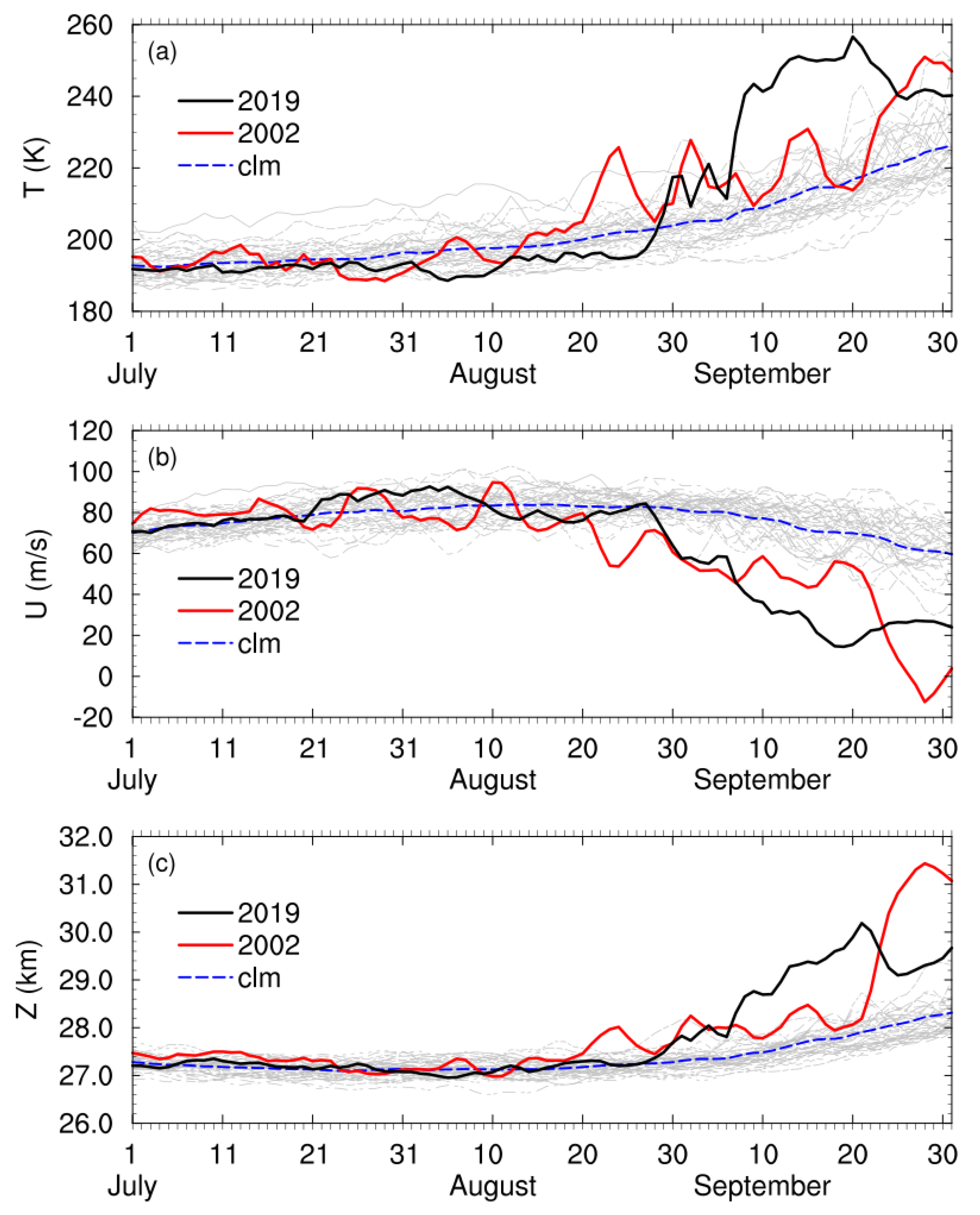
The time evolution of the Antarctic stratospheric polar vortex is shown in Figure 1. As mentioned in Rao et al. (2020) [16], the 2019 Antarctic SSW had very strong circulation changes, which were not weaker than the major event in 2002 and some major SSWs in the Northern Hemisphere. There were two warming processes in the life cycle of this 2019 Antarctic SSW event. During July-August-September (JAS) in 2019, the first warming of 10 hPa temperature over the polar cap occurred in late August, rising by about 20 K (Figure 1a). Meanwhile, the stratospheric polar night jet (PNJ) was disturbed markedly (Figure 1b). Then, the second warming followed in early September, with the temperature at the Pole increasing more than 30 K. The PNJ continued to weaken, reaching the minimum in mid-September. It is clear that the peak of temperature over the polar cap was the highest since 1979. As for the evolution of the geopotential height over the polar cap (Figure 1c), we can also see the significant weakening of the polar vortex during the 2019 Antarctic SSW, which was second only to that in 2002. Although the wind-reversal at 10 hPa did not appear at 60° S, the second strongest wind deceleration and the most significant warming do suggest that the Antarctic SSW in early September 2019 was, indeed, an unusual event with a very strong disturbance.

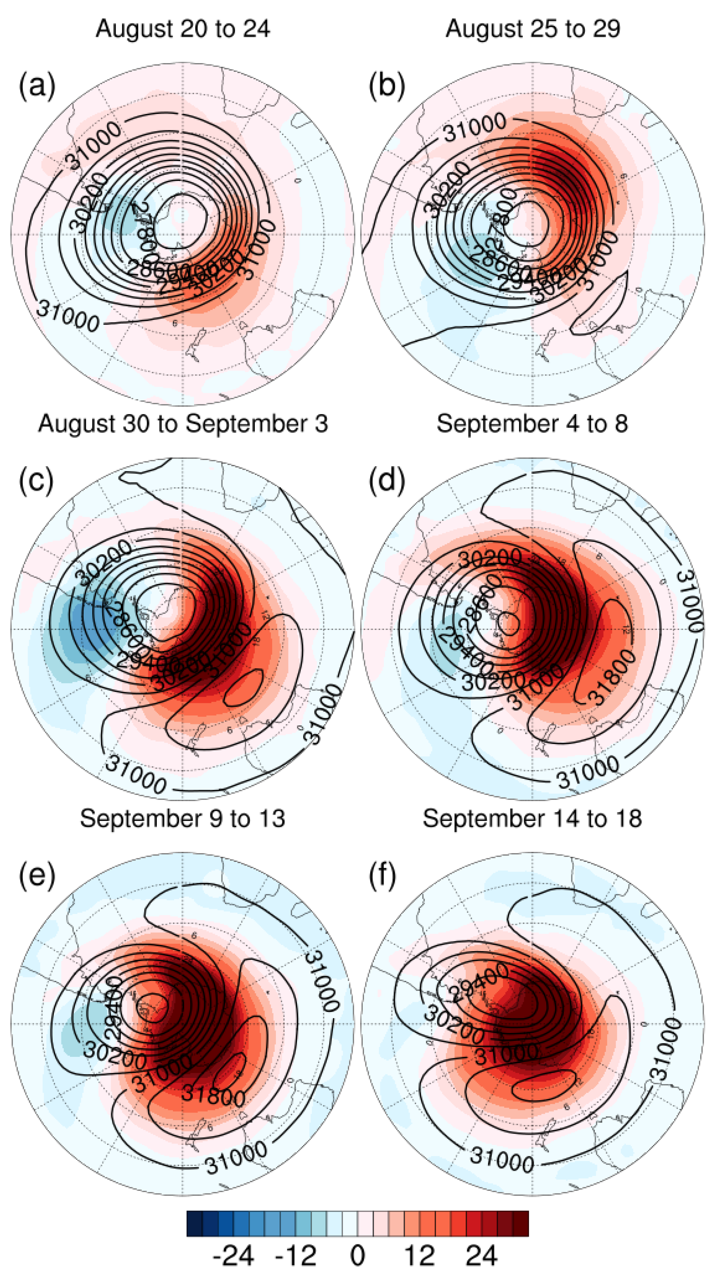
In addition to the dramatic change of the time evolution of circulation, the geometry of the polar vortex has also undergone great changes. Figure 2 shows the temporal–spatial distributions of geopotential height field and temperature anomalies at 10 hPa in the Southern Hemisphere. In late August, the polar vortex in the Southern Hemisphere was basically undisturbed, and the warming over the polar cap was also not marked (Figure 2a,b). From early to mid-September (Figure 2c–f), the polar vortex over the Southern Hemisphere was prominently disturbed and shifted toward the low latitudes, forming a clear wave-1 structure. Meanwhile, the warming also peaked in mid-September, occupying the entire Antarctic region.

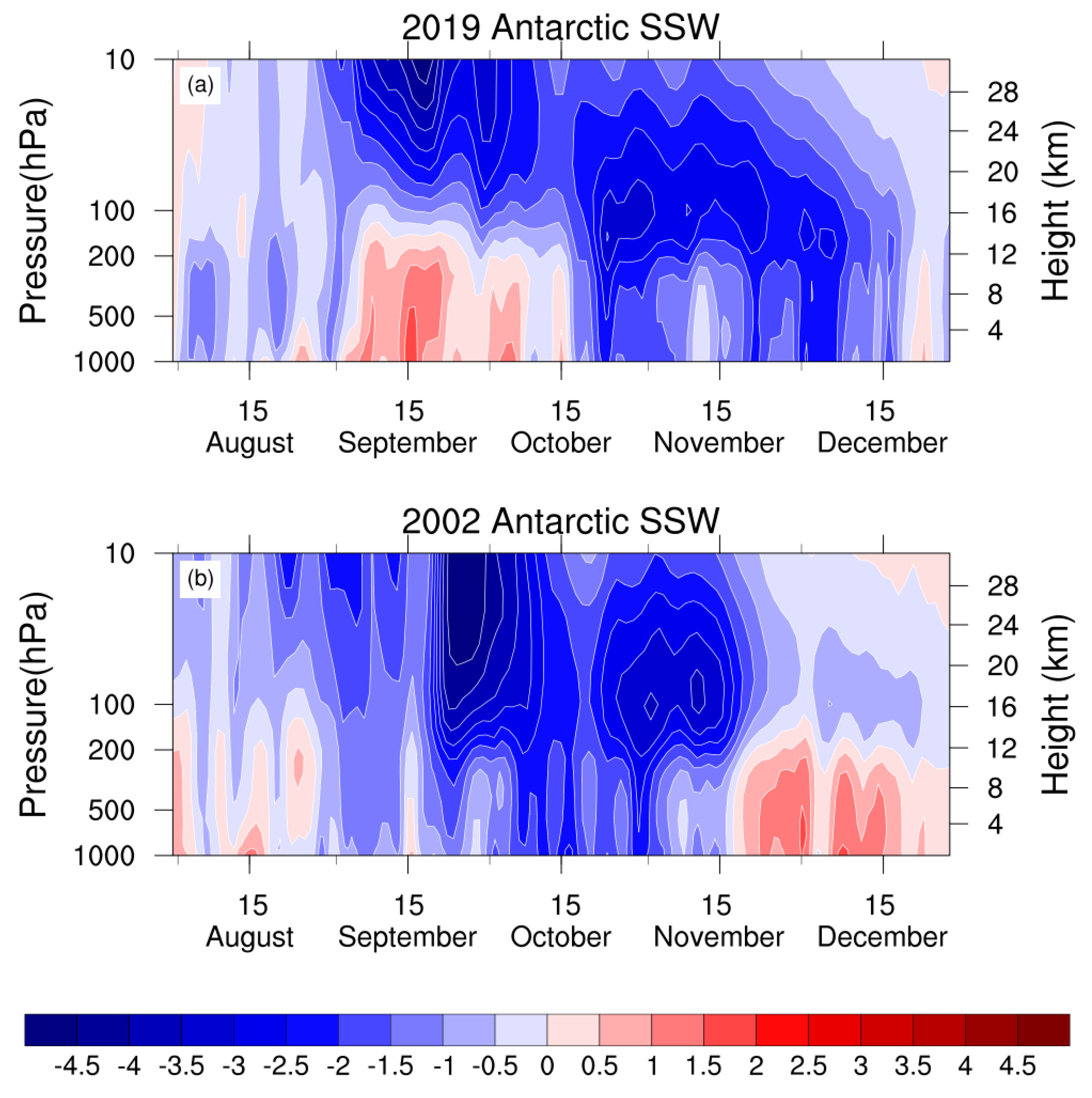
Accompanied by the clear shift of the polar vortex, this change also affects the lower-level circulation. Figure 3 shows the time-height evolution of the SAM from August to December in 2019 (Figure 3a) and 2002 (Figure 3b), respectively. It is clear that the SAM in the stratosphere turned significantly negative since September 2019, with a sudden stratospheric warming (Figure 3a). A distinctly negative SAM persisted in the stratosphere for about 40 days and began to propagate downward into the lower levels in mid-October, with a clear impact on the troposphere, lasting for nearly two months. Meanwhile, we can see that the downward influence of the SAM in 2002 also lasted for nearly two months, so the influence of the two Antarctic SSWs on the lower-level circulation was very significant and persistent. However, it should be noted that there was a significant difference in the evolution of the SAM in the two years. The vertical evolution of the SAM during the 2002 Antarctic SSW indicated an instantaneous response between the upper and lower levels, showing a barotropic mode. In contrast, the evolution of the SAM in the 2019 event showed a distinctly downward-propagation mode. It reflects that there are differences in the formation and downward-propagation mechanism of the two Antarctic SSWs.

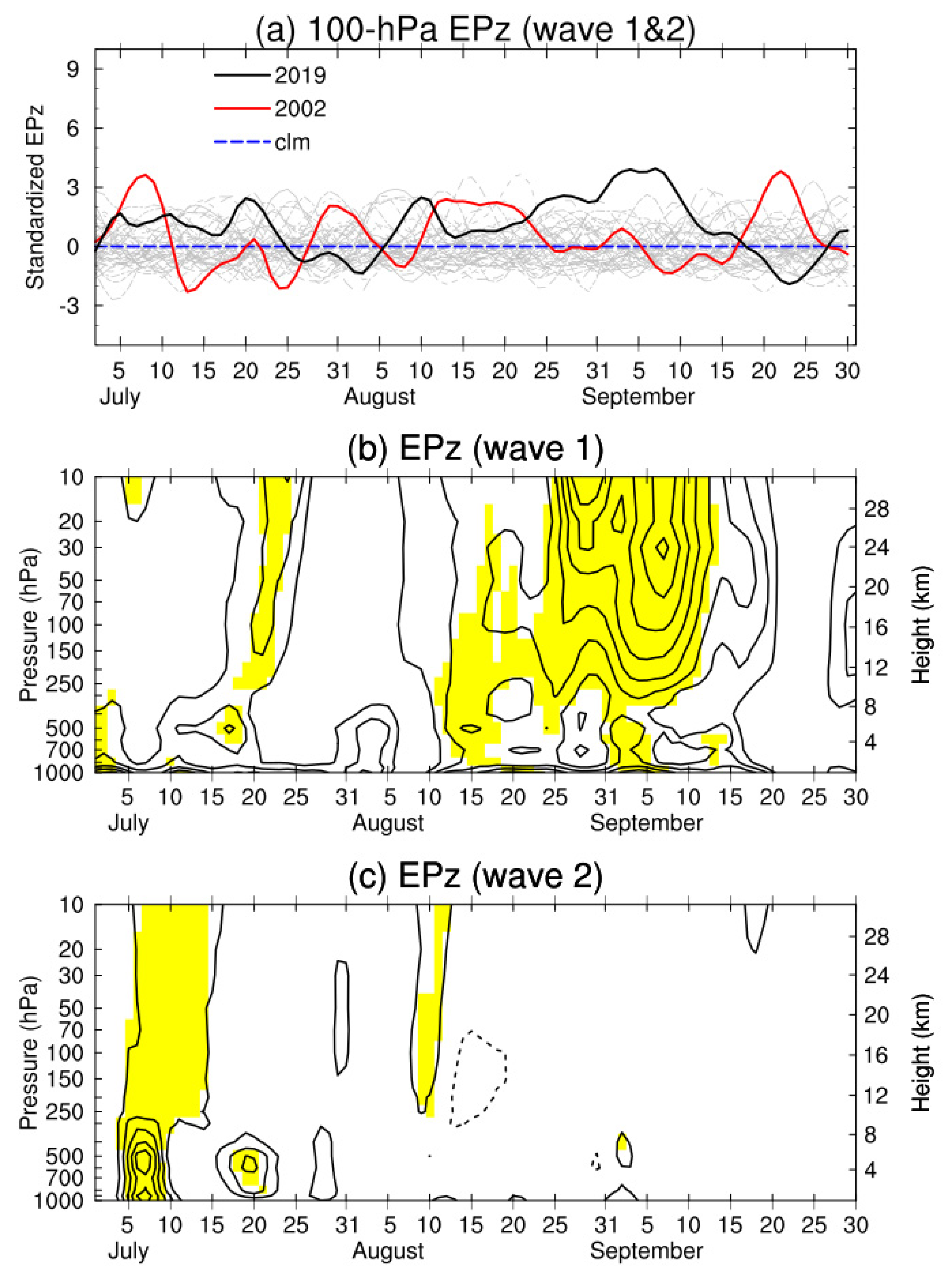
It has been shown theoretically that enhanced upward EP fluxes associated with planetary-scale waves play an important role in the occurrence of SSWs [31]. The results by Bao et al. (2017) [32] indicated that there exist several tropospheric circulation patterns that strengthen the tropospheric planetary waves preceding Arctic SSW events. It was found that the 2002 Antarctic SSW event was closely related to the enhancement of the tropospheric planetary waves [4,33]. Figure 4 illustrates the time series of the standardized upward EP fluxes (EPz; top panel) at 100 hPa over 40 years and time-height sections of the EPz of zonal wavenumbers 1 (W1; middle) and 2 (W2; bottom) at 60° S during the period of 2019, respectively. It can be seen that the upward wave flux in 2019 has been the strongest in 40 years from late August to mid-September (Figure 4a), which indicates that there must be a strong and persistent wave source in the troposphere. Moreover, the planetary wave activity of W1 was very strong through the period in 2019, especially from mid-August to mid-September (Figure 4b). This result is consistent with a recent study on the 2019 case [12]. The strongest stratospheric wave activity starting in late August corresponds to the occurrence of the disturbed polar vortex. In contrast, the stratospheric wave activity of W2 is very calm except for two pulses with moderate values in early July and early August (Figure 4c). Therefore, the occurrence of the 2019 Antarctic SSW can be attributed to the strong and persistent planetary W1.

The persistent strong planetary-scale W1 originated from the troposphere. It has been suggested that there could exist some tropospheric forcing to play a role in enhancing the planetary wave amplitudes [31]. Many studies have demonstrated that the warm SST anomalies near the equator can excite a Rossby wave train emanating poleward from the tropics [34]. 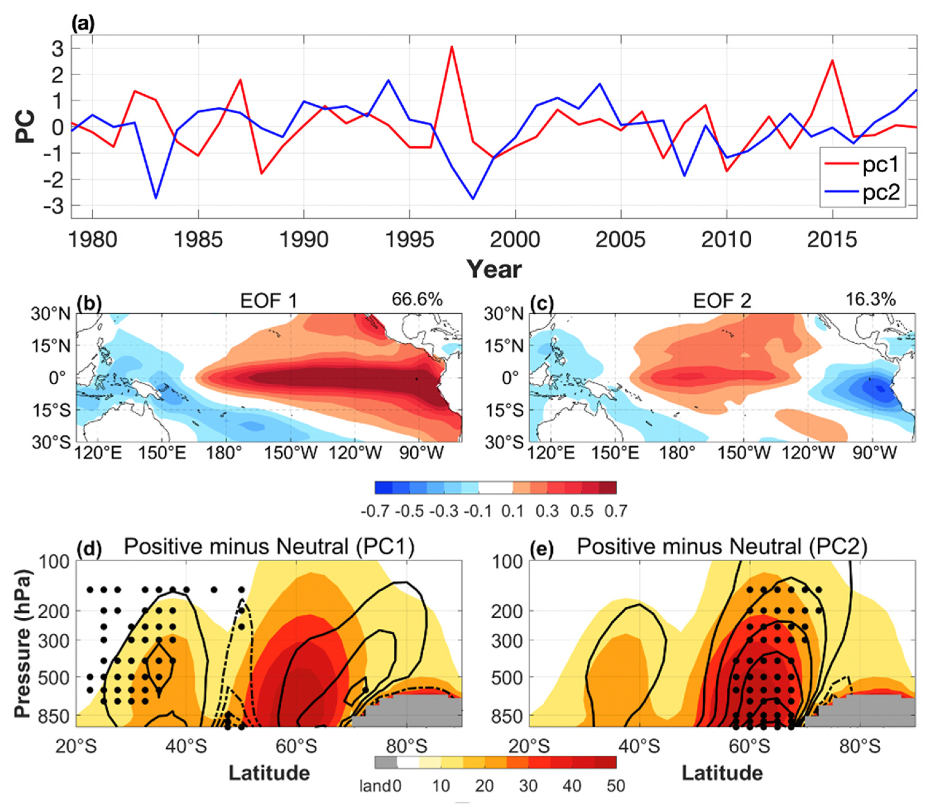Such a teleconnection of the El Niño Southern Oscillation (ENSO) to the extratropics can deepen the Aleutian low and strengthen the upward wave activity into the stratosphere in boreal winter [35], thus increasing the probability of SSW events [36]. Different from the Arctic SSWs appearing in boreal winter, the Antarctic SSWs in 2002 and 2019 occurred in September. Thus, we performed an EOF analysis on the tropical Pacific (10° S–10° N, 110° E–70° W) SST anomalies following Ashok et al. (2007) [37], but for JAS season during 1979–2019. The EOFs 1–3 explain 66.6%, 16.3%, and 5.8% of total variance, respectively. The first and second EOFs are unique according to the North test [38]. Figure 5a–c show the EOF1, 2, and their corresponding principal components (PCs). The EOF1 denotes a canonical ENSO-like pattern during austral late winter–early spring. The years with the significantly positive PC1 anomalies (values of standardized PC1 more than 1.0 standard deviation (SD)) include 1982, 1983, 1987, 1997, and 2015. The positive phase of EOF2 presents the Pacific SST anomalies with the central warming and the eastern cooling. Note that the central (eastern) Pacific warming during JAS season does not equal to a central (eastern) Pacific El Niño event during its growing phase. The years with the significantly positive PC2 anomalies (values of PC2 more than 1.0 SD) are 1994, 2002, 2004, and 2019. These four years all exhibit typically central Pacific warming.

Figure 5d,e show the difference of the JAS-mean tropospheric W1 amplitudes between the significantly positive years and the neutral years (absolute values less than 1.0 SD). The climatological-mean amplitudes of the tropospheric W1 maximize around 60° S. While the W1 amplitudes are significantly enhanced in the subtropics for EOF1 (Figure 5d), they do not enhance the climatological W1 at mid-high latitudes and thus do not disturb the polar vortex. A significant difference at mid-high latitudes only appears for EOF2 (Figure 5e), indicating the marked strengthening of the seasonal-mean tropospheric W1 at mid-high latitudes. The strengthened convection associated with central Pacific warming would excite the stationary Rossby wave. Then, the Rossby wave would enhance the extratropical seasonal-mean W1 by propagating on the sphere and interfering constructively with the climatological-mean W1 [39,40,41].

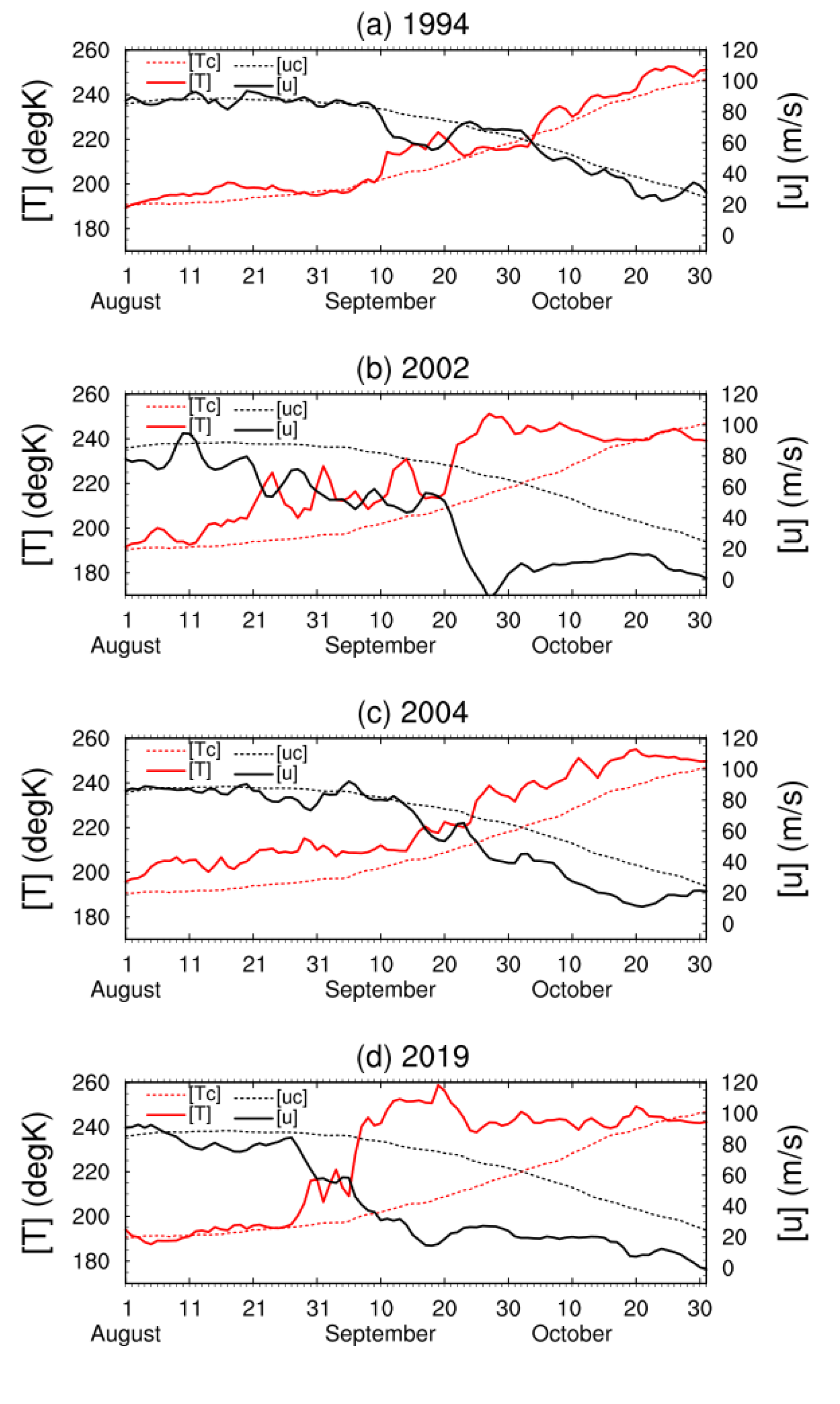
Based on the impact of central Pacific warming, we examined the evolution of four significant warming years. As shown in Figure 6, in addition to the unusual weakening of the Antarctic vortex in 2002 and 2019, there were also clear disturbances of the Antarctic vortex in 1994 and 2004. In addition, it is noted that since the subsequent wind field was still easterly for a long time, these disturbances were obviously not caused by the final warming. Besides, we have checked the time evolution of the Antarctic vortex from August to October in other years (not shown). It is found that the Antarctic vortex generally has a disturbed event in the year with positive PC2 (e.g., 1992, 1994, 2001) in Figure 2, but usually does not have obvious disturbances in the year with negative PC2 (e.g., 1983, 1997–1999, 2009). These results and previous studies [40,42] reflect that the central Pacific warming does play a role in the disturbance of the polar vortex in the Southern Hemisphere. Therefore, the 2019 Antarctic SSW was somewhat influenced by the significant central Pacific warming.

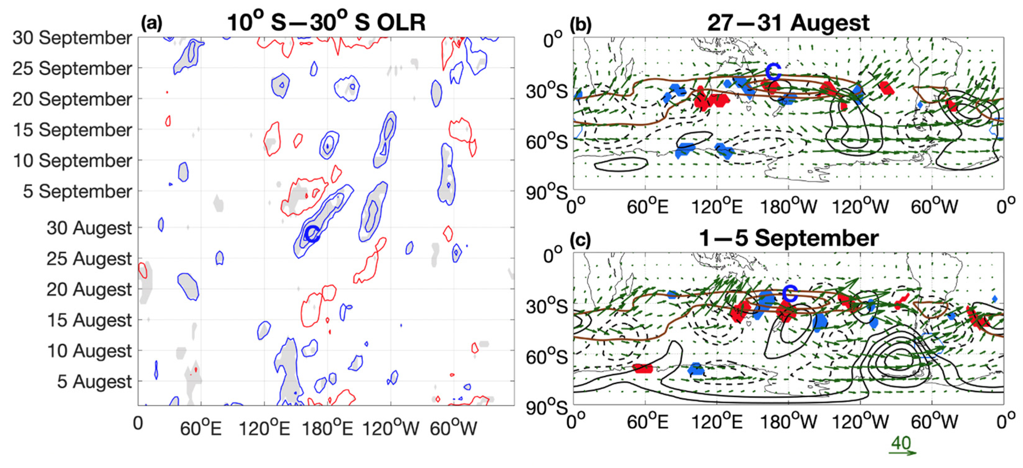
Nishii and Nakamura (2004) [2] found that the anomalous deep convection over the SPCZ in mid-September 2002 forced a Rossby wave train that formed a tropospheric blocking ridge over the Southern Atlantic. This blocking enhanced the upward propagating of planetary waves and thus led to the 2002 SSW. We examined the time evolution of the convection activities along 10° S–30° S in 2019 (Figure 7a). Note that the seasonal (JAS) mean is subtracted in Figure 7. The anomalous deep convection over the SPCZ appeared from 25 August to 5 September, propagating southeastward and crossing the dateline slowly. The timing of the anomalous deep convection coincided with the strengthening of the upward propagation of W1 (Figure 4b) and the first stratospheric warming stage (Figure 1a). The positive Rossby wave source associated with the anomalous deep convection was attributed to the large absolute vorticity gradients associated with the subtropical jet [24]. In late August and early September, the Rossby wave source near the dateline excited a Rossby wave train propagating eastward along the subtropical jet and another Rossby wave train propagating southeastward into the South Pacific denoted by the wave activity flux in Figure 7b,c. The wave train propagating southeastward was strengthened due to the feedback from transient eddies and formed a planetary-scale ridge (Figure 7c). The resultant planetary-scale anomalous ridge over the southeast Pacific indicates a strengthening of the tropospheric W1, as the anomalous ridge constructively interferes with the climatological-mean W1 ridge (not shown). The result of the wave train is consistent with that in Shen et al. (2020) [14].

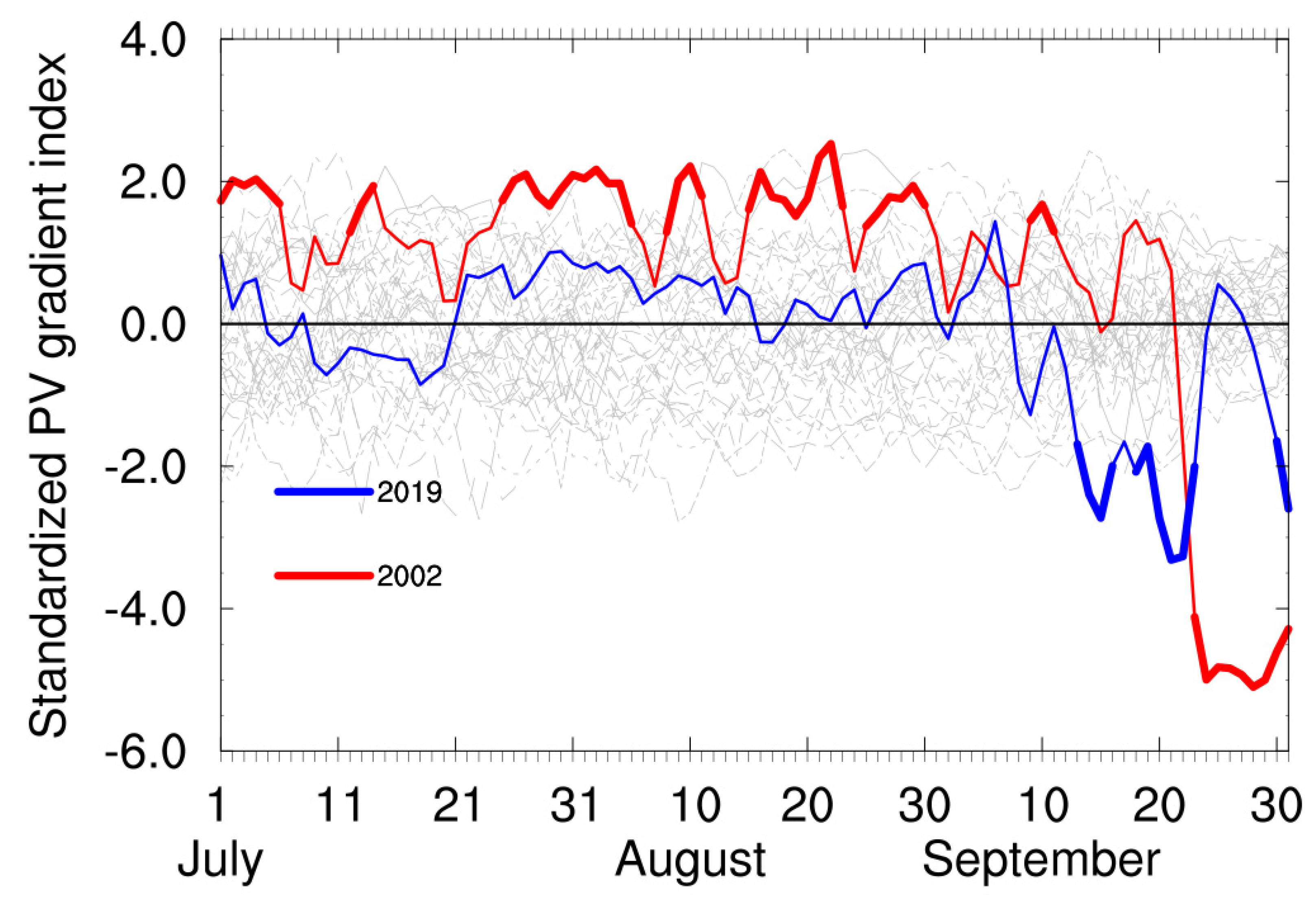
Both the central Pacific warming and intraseasonal anomalous deep convection played important roles in the two Antarctic SSWs in 2002 and 2019—why did the 2019 Antarctic SSW fail to meet the standards of major events? Figure 8 shows the evolution of the meridional PV index from 1 July to 30 September over 40 years. It is clear that the meridional PV index of the 2019 SSW remained small before the SSW until it turned significantly negative after the warming. However, the meridional PV index of the 2002 event was significantly positive, which is distinctly different from that in 2019. It should be noted that the sharpening of the PV gradient along the vortex edge can increase the local refractive index there and facilitate wave flux at the lower levels to enter the stratosphere at high latitudes [29].

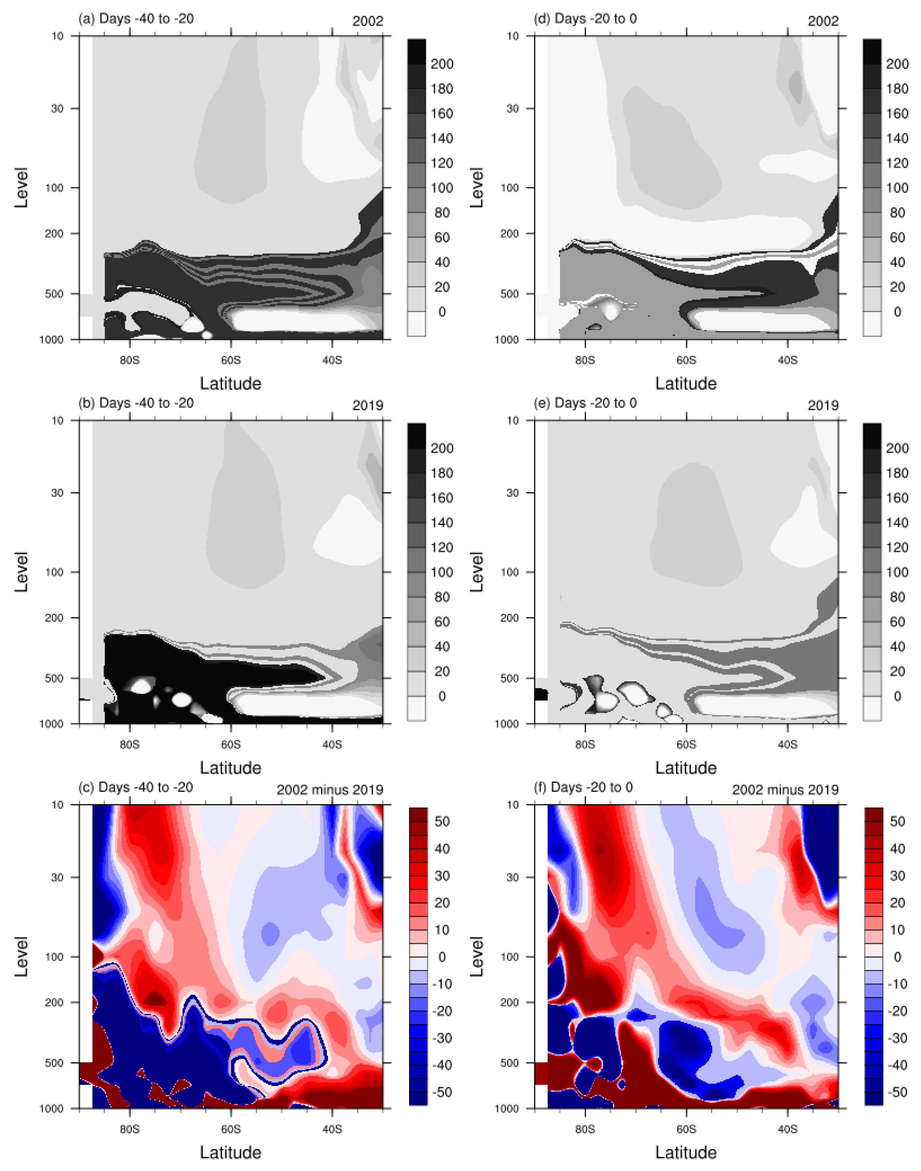
In addition, the W1 refractive index was also diagnosed, which is shown in Figure 9. The W2 refractive index showed similar results (not shown). According to the temperature evolution in Figure 1, September 20 and September 5 were selected as the onset dates of the two significant warming events in 2002 and 2019, respectively. Compared with the 2019 event, the refractive index showed a more pronounced vertical structure in the polar stratosphere from days −40 to −20 before for the 2002 warming, accompanied by a more positive index. During days −20 to 0, the difference of index in the middle stratosphere was more distinctive. Waves are preferentially refracted toward regions with a more positive index of refraction [28]. As a result, the stratospheric state prior to the 2002 Antarctic SSW might have been in a more favorable state for wave activity to propagate upward to the polar stratosphere for a long time, which caused the polar vortex in the Southern Hemisphere to be disturbed for a long time. It matches the fact that PNJ in 2002 has been weakening, and the minor warming has appeared many times since mid-August before the occurrence of the major Antarctic SSW (Figure 1). Since the strong PNJ may inhibit the upward propagation of a planetary wave [43], the favorable stratospheric dynamics and the weak polar vortex in the preconditioning of the 2002 Antarctic SSW provide favorable conditions for the occurrence of the major event. However, since the preconditioning of the minor SSW event in 2019 was not as ideal as that of the 2002 event, the polar vortex was basically not disturbed and maintained at a strong level. Therefore, even though the tropospheric wave source was almost as strong as the 2002 event, it was more difficult to trigger a major SSW.

4. Summary and Discussion

In the present study, we have analyzed the occurrence of the Antarctic SSW event in 2019 since the first major Antarctic SSW event was recorded in 2002. We have also discussed possible contributions of the seasonal-mean SST and intraseasonal deep convection forcings to the amplification of the tropospheric W1 at mid-high latitudes and their impacts on the occurrence of this SSW event. Moreover, we have analyzed the possible reasons why the 2019 Antarctic SSW could not be a major event but the 2002 event was.

The enhanced deep convection on intraseasonal time scale over the SPCZ played a potential role in 2019 similar to that in 2002, which was revealed by previous work [2]. The strong and persistent deep convection over the SPCZ excited a Rossby wave train to favor the formation of a prominent anomalous ridge, which significantly strengthened the tropospheric W1 for a long time. Here, we emphasize that the tropical central Pacific warming may provide an important climatic preconditioning both for 2002 and 2019 SSW events. The central Pacific warming has evident effects on strengthening the tropospheric W1, which could propagate upward to disturb the stratospheric polar vortex. The impacts of central Pacific warming on the tropospheric W1 and the stratosphere in the Southern Hemisphere have also been mentioned in previous studies [39,40,41,42]. In addition, the warming SST around the central Pacific may also provide favorable conditions for anomalous strong and continuous convection. However, it should be noted that it is very difficult to quantitatively compare the relative contributions of the two forcings—intraseasonal deep convection over the SPCZ and central Pacific warming. Firstly, the two forcings do not directly affect the stratosphere, but provide favorable conditions. Secondly, considering the time scales of the two forcings are quite different, they may not be independent. Finally, limited by the shortage of sample size, general results are difficult to obtain. All of these have given rise to great obstacles in clarifying the relative contributions of the two forcings. Therefore, further quantitative research is needed in the future.

When summarizing the research results for the 2002 SSW event, it was concluded that “Indeed there may well have been no identifiable external cause: it may simply be best just to regard it as a random event, associated with the chaotic nature of atmosphere dynamics.” [44]. The present study suggests that the tropical central Pacific warming might be regarded as an identifiable external factor for an Antarctic SSW prediction. However, there are some exceptional years (e.g., 1988, 2007, 2012) exhibiting minor weakening of the Antarctic vortex without significant central Pacific warming. It is indicated that the tropical central Pacific warming is a responsible but not necessary cause for the disturbance of the Antarctic vortex. There are other potential factors (e.g., Quasi-Biennial Oscillation (QBO), solar cycle, sea ice, and Indian Ocean Dipole) that may influence the minor weakening of the Antarctic vortex.

Both the seasonal-mean and intraseasonal wave signals provided the conditions for the occurrence of the Antarctic SSWs in 2002 and 2019. Moreover, SSW preconditioning could also come from the stratospheric precursor [27,29,45,46,47]. However, the stratospheric state before the 2019 Antarctic SSW was not ideal as that of the 2002 event. As a result, the PNJ continued to weaken due to the favorable stratospheric dynamics for a long time before the occurrence of the 2002 Antarctic major SSW. Additionally, the unideal stratospheric state in 2019 not only made the PNJ prior to the minor warming not disturbed, but also somewhat restrained the impact of a strong troposphere wave on the polar vortex. Therefore, the internal stratospheric state may be an important reason why the 2019 Antarctic SSW did not meet the standard of a major event.

Hurwitz et al. (2011) [40] found that there was a significant response of the Antarctic stratosphere to the central Pacific El Niño in austral late spring, but no response to cold tongue El Niño. Lin et al. (2012) [41] obtained a similar conclusion based on the maximum covariance analysis from late winter to early summer. Gray et al. (2005) [48] indicated that the anomalous easterlies in the equatorial upper stratosphere contributed to the development of the 2002 Antarctic SSW, and Shen et al. (2020) [14] also pointed out that the upper stratospheric QBO provides a favorable stratospheric background for the occurrence of the 2019 Antarctic SSW. Meanwhile, the conditions of QBO and central Pacific warming were similar in 2002 and 2019, and some studies also pointed out that the joint effect of QBO and ENSO will have a role on the Antarctic polar vortex [49]. Thus, the joint effect of the eastern phase of QBO and central Pacific warming may be worthy of further study.

Note that the impact of QBO on the polar vortex is mainly on the seasonal time scale, while the evolution of stratospheric circulation in 2002 and 2019 was different for a long time from late winter to early spring. Therefore, although there were some works that suggested the impact of the QBO on the Antarctic polar vortex [50,51,52], the modulation of the QBO and the equatorial zonal winds in the upper stratosphere on the Antarctic stratospheric polar vortex in different seasons still needs specific investigations.

According to the projection, the more frequent central Pacific warming events indicated by the warming in the tropical western Pacific [53] and the warming in the SPCZ area under future anthropogenic forcing imply there may be an increased probability of occurrence of Antarctic SSW. Meanwhile, the internal stratospheric state should also be noted in the future studies of Antarctic SSW.