Article

Analysis of Chemical Composition Characteristics and Source of PM2.5 under Different Pollution Degrees in Autumn and Winter of Liaocheng, China

1
State Key Laboratory of Environmental Criteria and Risk Assessment, Chinese Research Academy of Environmental Sciences, Beijing 100012, China
2
Chinese Academy for Environmental Planning, Beijing 100012, China
*
Authors to whom correspondence should be addressed.
Atmosphere 2021, 12(9), 1180; https://doi.org/10.3390/atmos12091180
Submission received: 19 July 2021 / Revised: 31 August 2021 / Accepted: 6 September 2021 / Published: 13 September 2021
(This article belongs to the Section Air Quality)

Abstract

:
Analysis of chemical composition characteristics of PM2.5 under different pollution degrees can reveal the changes of pollution sources. In order to make clear the evolution process of PM2.5 compositions in autumn and winter, PM2.5 samples were continuously collected and analyzed at Liaocheng city, China. The collected samples were classified as clean days (CLD), mild-moderate pollution days (MMD) and severe-serious pollution days (SSD). It was concluded that with the increase of pollution degrees, the concentrations of water-soluble ions and carbon components increased significantly, while elements only increased slightly. In addition, as the pollution degrees increased, the percentage of NO3, SO42− and NH4+ increased significantly, from 23.0% in CLD to 49.0% in SSD, while the percentage of other components decreased, especially crust material. The PMF analyzed results showed that secondary transformation (36.7%), combustion sources (20.4%), secondary organic aerosols (SOA) (11.7%), vehicle sources (11%), dust (10.5%) and industrial processes (9.7%) were the main sources of PM2.5 during autumn and winter in Liaocheng. The contribution of secondary transformation reached 57% at the SSD level, which indicated that it was the main reason for the increase of PM2.5 concentrations. The air mass mainly came from five paths to Liaocheng. The secondary transformation contribution of the air mass with short transmission distance was higher, while the contribution of the dust was higher from the long distance.

1. Introduction

In recent years, China has experienced rapid economic developments along with serious air pollution problems, especially extreme haze episodes. Since 2013, with the formulation and implementation of a number of air pollution prevention and control measures, such as “Air Ten” and “Winning the Battle to Protect the Blue Sky” [1,2], the emission of air pollutants in China has decreased significantly, and the air quality has improved, but PM2.5 is still the primary pollutant in most cities [3]. The chemical composition of PM2.5 is very complex and has an important impact on visibility, climate and human health. At present, numerous analyses of chemistry compositions and source appointment of PM2.5 have been carried out in typical polluted areas in China like Beijing-Tianjin-Hebei and surrounding areas [4], the Yangtze River Delta [5] and the Pearl River Delta [6] and lots of cities like Beijing [7], Tianjin [8], Shijiazhuang [9], Xingtai [10], Jinan [11], Shanghai [12] and Guangzhou [13]. Sulfate, nitrate and ammonium were found to be the major components of water-soluble inorganic ions, which accounted for 30–80% of PM2.5. Carbonaceous components are also important constituents of PM2.5, and OC contains a large number of carcinogenic, teratogenic and mutagenic components [14]. Elements were divided into crustal elements and anthropogenic pollution elements, including trace heavy metals, although their concentration is relatively low but harmful to the human body [15]. An analytical model of particulate matter receptor method is one of the common tools in the study of source appointment [16]. The positive definite matrix (PMF) and its analytic results are also objective sources of information. Additionally, the PMF model can provide the time series of various pollution sources’ contributions. Therefore, the PMF model was selected in this paper to analyze the sources of PM2.5 in Liaocheng.
Shandong Province is an area with a high concentration of air pollutants and frequently encountered haze episodes. Liaocheng is located at the northwest inland area of Shandong Province, and it is one of the important transport channels of air pollution in the “2 + 26” cities area. The air pollution problem of Liaocheng has been widely concerned because of its low ranking in the Shandong province. Currently, the research of PM2.5 in Liaocheng mainly focuses on the analysis of the characteristics of chemical components and sources [17,18,19], but there was no report on the characteristics and source apportionment of PM2.5 under different pollution degrees, as well as research in the whole autumn and winter period. Therefore, this study analyzed the characteristics and sources of PM2.5 under different pollution degrees in the autumn and winter of Liaocheng in order to provide data support and scientific support for air pollution control in Liaocheng.

2. Materials and Methods

2.1. Sampling of PM2.5

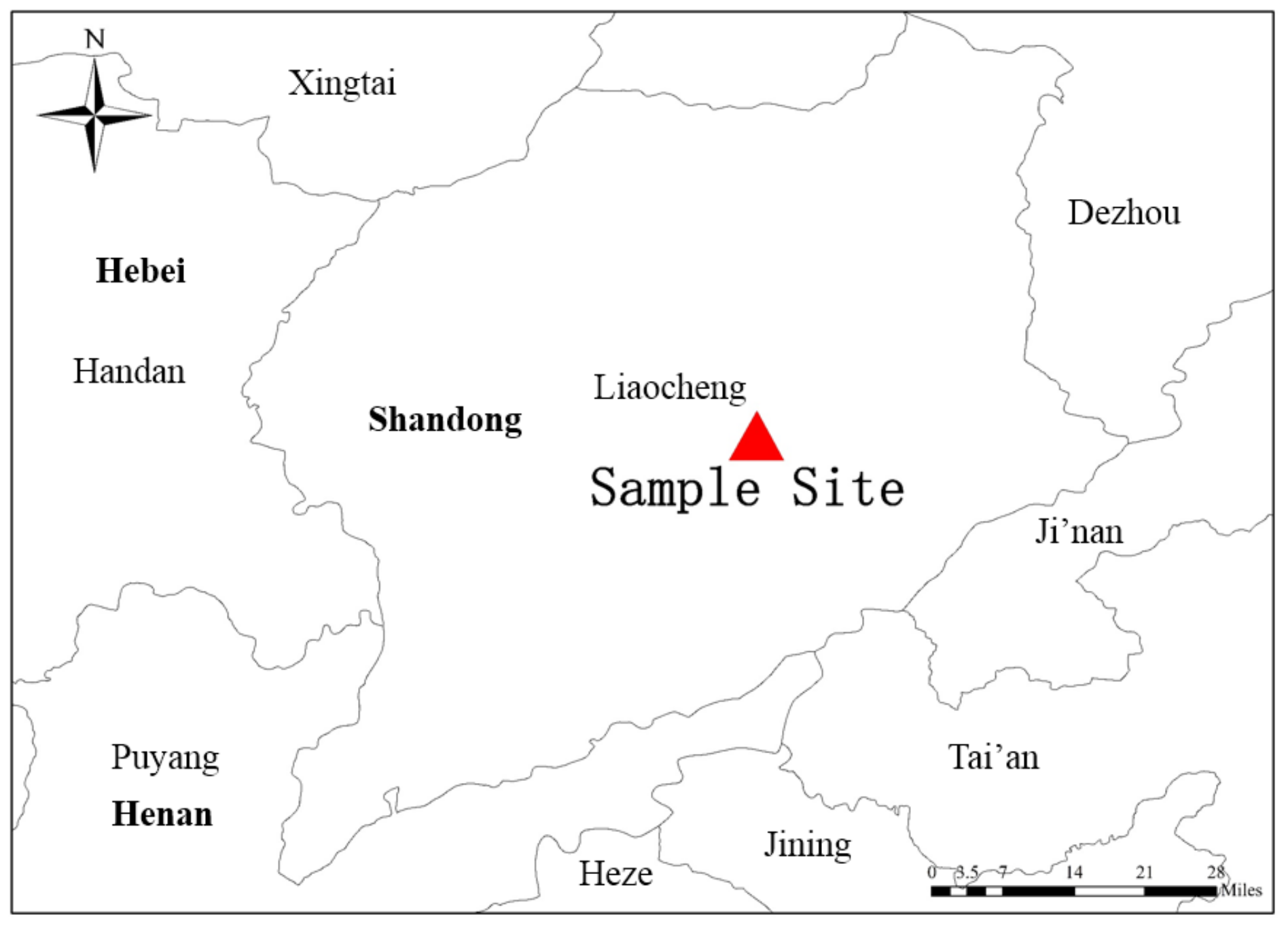
2.1.1. Sampling Position, Period and Samples Collection

PM2.5 was collected at the campus of Liaocheng University, located east of Liaocheng (34.43° N, 115.99° E) and is shown in Figure 1. The instruments used in this study were installed on the rooftop (15 m above ground) of NO.4 Experimental Building. There were no tall buildings and obvious pollution sources around the sampling site, which could objectively reflect the air pollution situation in Liaocheng. Two high-volume samplers (TH-150C, Tianhong Instrument Co. Ltd., Wuhan, China) were used to collect PM2.5 samples, and the flow rate was set to 100 L·min−1 during the sampling process. Quartz and polypropylene films were loaded to capture PM2.5, and both were 90 cm in size. After sampling, the filter samples were placed in the refrigerator at −4 °C for preservation. The sampling time was 109 days, from 15 October 2017 to 31 January 2018, while the sampling duration for each sample was 23.5 h, from 10:00 a.m. to 9:00 a.m. the next day, and a total of 109 PM2.5 samples were collected. During sampling periods, the machine failure period and invalid data were removed, and a total of 105 groups of effective samples were obtained.

2.1.2. Quality Assurance and Quality Control of Sampling

The samplers were calibrated before the sampling process, the flow-rate range of the samplers was from 60 to 150 L/min with an accuracy of ±2.5%, and the relative error of the flow rate was less than 2%. The quartz films were first calcined at 450 °C for 5 h, and polypropylene films at 60 °C for 3 h in order to remove the organics and other impurities on the films. Then, the films were packed into aluminum foil papers and placed in a constant temperature and humidity chamber at 25 °C and 50 °C of 5% relative humidity for 24 h. Then, the films were sealed in film boxes at a temperature of 20 °C. Three blank films were reserved as the blank samples to correct the data of each sample in order to guarantee the accuracy and reliability of the analyzed data of the collected samples.

2.2. Chemical Components Analysis of PM2.5

2.2.1. Water-Soluble Ions

Before analysis, polypropylene films were extracted ultrasonically by 20 mL of ultrapure water for 20 min, and then water-soluble matter was filtrated and stored at 4 °C. Ion chromatography (Universal ICS-90, Metrohm Company, Herisau, Swiss) was used to analyze the inorganic ions, which included chloride (Cl), nitrate (NO3) and sulfate (SO42−), sodium (Na+), ammonium (NH4+), potassium (K+), magnesium (Mg2+), calcium (Ca2+) and fluoride (F) [20,21,22].

2.2.2. Carbonaceous Species

A circular quartz filter with an area of 0.558 cm2 was used to determine organic carbon (OC) and elemental carbon (EC) concentrations by a thermal/optical carbon analyzer (Model 2008; Desert Research Institute, Reno, NV, USA) [23,24,25,26].

2.2.3. Inorganic Element

Six quartz filters (10.9 cm2 each) were placed in a high-pressure Teflon digestion vessel, digested with a mixture of ultra-high purity acids (11.1% HNO3/33.5% HCl) and then heated in a microwave system. The microwave system was ramped to 200 °C and was retained at this temperature for 30 min. After the digestion process, metal components, such as Li, Be, Mg, Ti, V, Cr, Mn, Fe, Co, Ni, Cu, Zn, As, Se, Mo, Cd, Sn, Sb, Ba, Hg, Pb, Bi, Ca, K, Mg, Na, were determined using Inductively Coupled Plasma-Mass Spectrometry (7700 Series ICP-MS, Agilent Technologies Inc., Palo Alto, CA, USA). In addition, the concentrations of Al and Si were determined by Inductively Coupled Plasma Atomic Emission Spectrometry (8300 ICP-AES, PerkinElmer company, Boston, MA, USA) [27,28,29,30].

2.2.4. Quality Assurance and Quality Control of Chemical Components Analysis

Strict quality control and quality assurance measures were used in the chemical components analysis process. A three field blank was collected, and the laboratory blank was also analyzed. For each batch of samples, a blank addition criterion was added (water-soluble ions and inorganic elements). Recovery as well as calibration and quantification were performed using external standard solutions, the recovery rate of calibration was between 80% and 120%. The correlation coefficients of standard curves were all higher than 0.99. For every 10 samples, a calibration median point was analyzed. If the deviation of the calibration median point was greater than 20%, the curve was redrawn.
For carbonaceous species, the background contamination was regularly monitored by blank tests, which were used to validate and correct the corresponding data. Calibration of the analyzer was done before and after sample analysis every day. The first sample was analyzed every ten samples again, and the precision had to be less than 5%.

2.3. Data Analysis Method

2.3.1. Online Data Source

Air quality data were obtained from China’s air quality online monitoring and analysis platform (http://www/aqistudy.cn/historydata, accessed on 18 July 2021), and meteorological data were obtained from the National Oceanic and Atmospheric Administration (ftp://arlftp.arlhq.noaa.gov/pub/archives/gdas1/, accessed on 18 July 2021), which are open-source databases for research.

2.3.2. Analysis of Secondary Pollution

Secondary formation is an important reason for PM2.5 pollution. Sulfate and nitrate are the main products of secondary inorganic formation in PM2.5, and their components are related to the oxidation efficiency of SO2 and NO2. Usually, secondary formation rates of SO2 and NO2 are characterized by SOR (sulfate oxidation rate) and NOR (nitrate oxidation rate) [31,32], which can be calculated by the following Equations (1) and (2):
SOR = [SO42−]/([SO42−] + [SO2])
NOR = [NO3]/([ NO3] + [NO2])
where [SO42−] and [NO3] are concentrations in PM2.5, μmol/m3; [SO2] and [NO2] are the concentrations of the gas phase, μmol/m3.
Secondary organic carbon in the atmosphere is formed by photochemical reactions or gas-particle conversion of volatile and semi-volatile organic compounds. The degree of secondary carbon pollution can be characterized by indicators like OC/EC and SOC/OC. The higher the ratio, the more serious the secondary pollution. SOC concentrations were determined by the EC tracer method following Equations (3) and (4) [33,34].
POC = EC × (OC/EC)min
SOC = OC − POC
where OC and EC are measured concentration, (OC/EC) min is the minimum OC/EC ratio in the sampling period, POC and SOC represent the estimated primary OC and secondary OC, respectively.

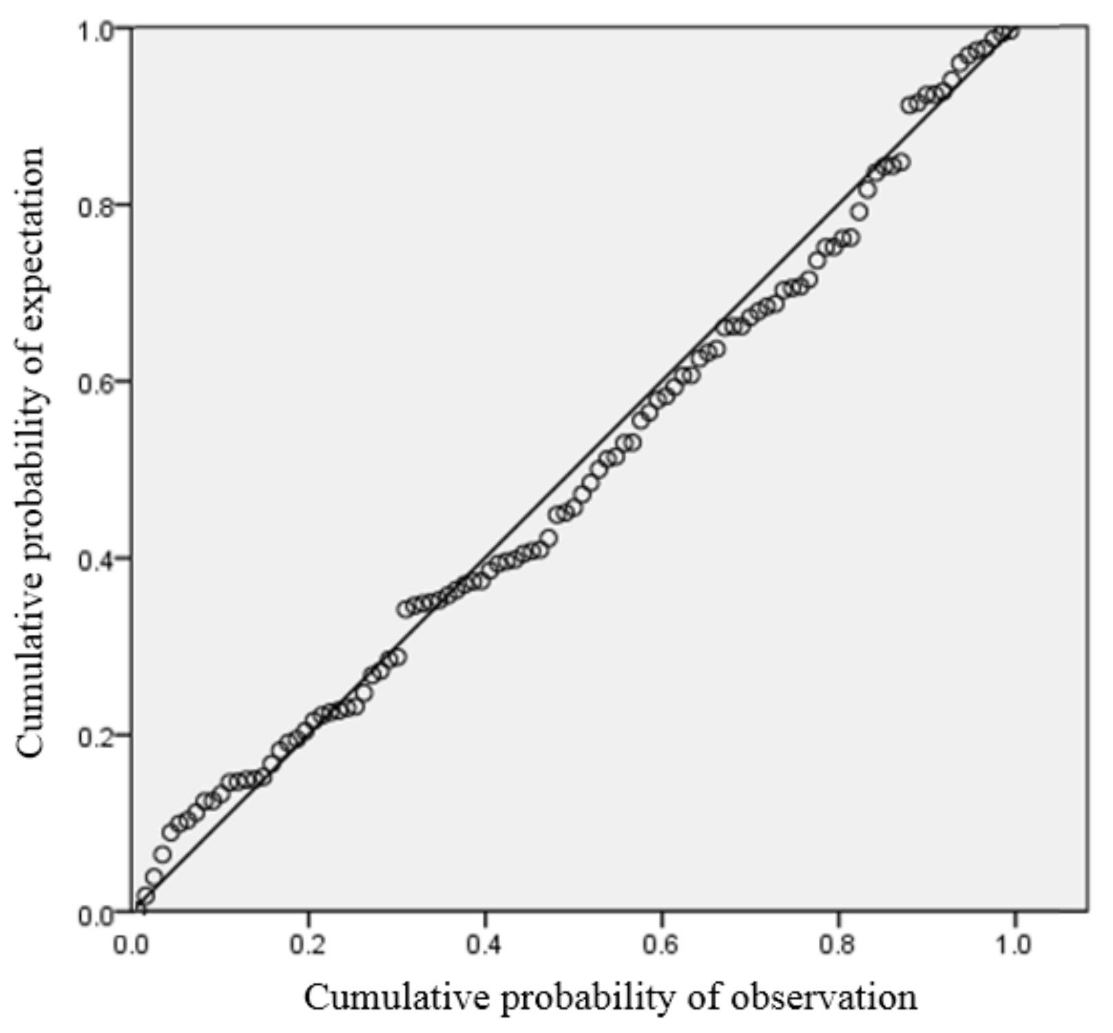
2.3.3. Positive Matrix Factorization Analysis

Positive Matrix Factorization (PMF) is a multivariate factor analysis tool that decomposes a matrix of sample data into two matrices: factor contributions and factor profiles [35,36]. With measured source profile information and emission inventories, the source type is determined. In this study, the EPA PMF 3.0 program was used for PMF analysis. The PMF model can be expressed as:
X i j = j = 1 p g i k × f k j + e i j
where Xij is matrix X of i by j dimensions, i is the number of samples and j is the number of chemical species, p is the number of factors, f is the species profile of each source, g is the amount of mass contributed by each factor to each individual sample, and eij is the residual for each sample/species. Q is an object function, and a criterion for the model, which is defined as:
Q = i = 1 n j = 1 n ( e i j / u i j ) 2
Qtheorical = I × jp × (I + j)
where uij is the uncertainty of the j th component in the i th sample.

2.3.4. Back Trajectory and Clustering Analysis

The 24 h backward trajectories of air mass during the pollution processes were investigated by the Hybrid Single Particle Lagrangian Integrated Trajectory (HYSPLIT) (http://ready.arl.noaa.gov/HYSPLIT.php, accessed on 12 July 2021) model developed by the National Oceanic and Atmosphere Administration (NOAA), and the ARL archives of the NOAA were used as the meteorological input data in this study. In this study, the model started at a height of 100 m above ground level with a time interval of one hour and set hourly 72 h back trajectory starting from the sampling site. Based on the results of the backward trajectory analysis, the trajectories and pollution concentrations were used for cluster analysis by MeteoInfo Map, which is an open-source geographic information system and scientific computing environment software.
Cluster analysis is an objective classification method to study multiple elements (or variables). It looks for a statistical quantity that can objectively reflect the distance relationship between samples and then divides samples into several categories according to the statistical quantity. The clustering method based on airflow trajectory is to group a large number of airflow tracks according to their spatial similarity (transmission velocity and direction). In this study, the Angle Distance algorithm provided by TrajStat software was used to cluster the airflow trajectory, and total spatial variance (TSV) was used to judge the classification quality. The principle is as follows: the TSV of the first several classification steps increases rapidly and then increases slowly. When the categories are divided to a certain number, TSV increases rapidly again, indicating that the merged categories are different. The classification merger is over, and the categories before the merger are the classification results. The average trajectories of these categories are the main flow trajectories of the target point in the analysis periods.

3. Results and Discussion

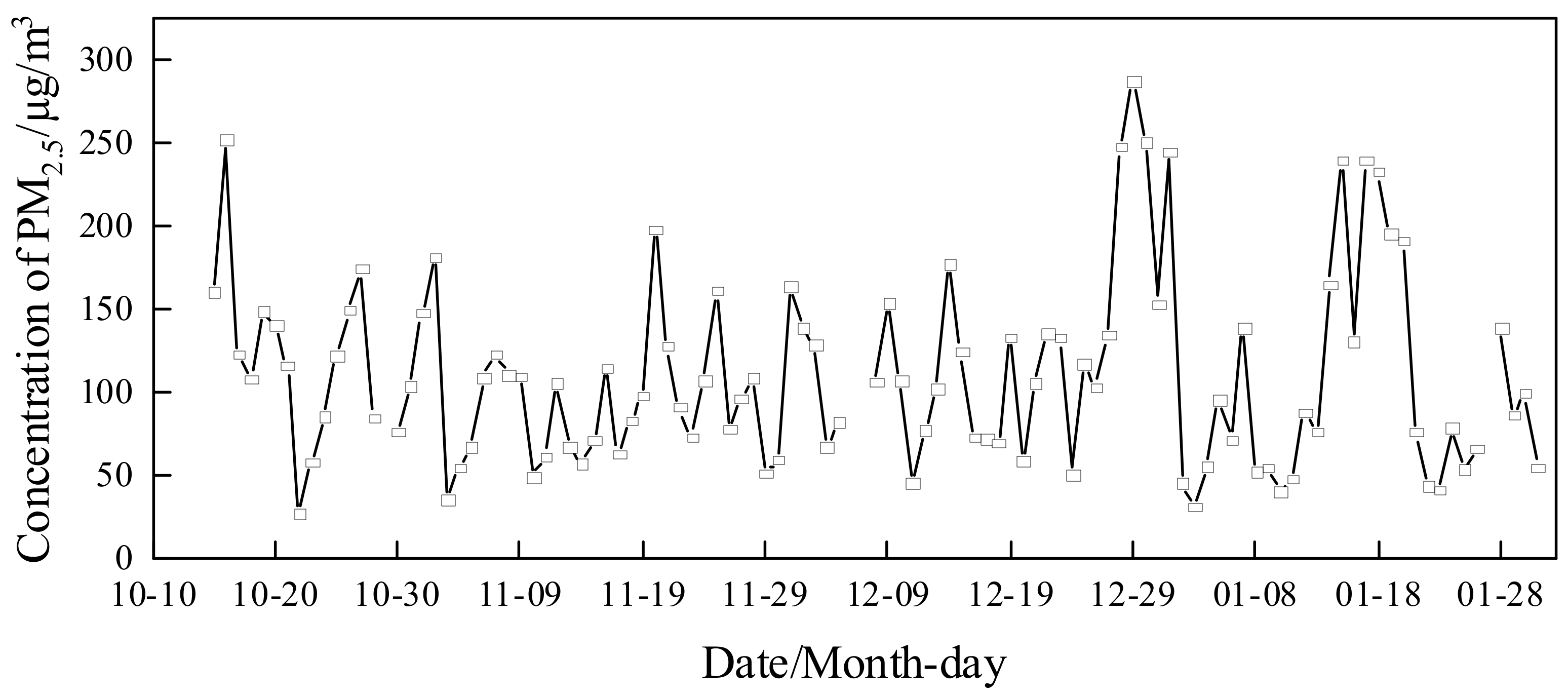
3.1. Analysis of Mass Concentrations of PM2.5 and the Meteorological Conditions

The daily average concentrations of PM2.5 and the meteorological conditions are shown in Figure 2 and Table 1, respectively. The average concentration of PM2.5 was 109.7 μg/m3, ranging from 26.7 to 286.3 μg/m3 with a standard deviation of 56.8 μg/m3. Compared with the Chinese National Ambient Air Quality Standard (NAAQS) (daily standard: 75 μg/m3), this value exceeded NAAQS 0.46 times, and the peak concentration appeared in December 29, exceeding the standard 2.82 times. Liaocheng is one of the “2 + 26” cities which are heavily polluted in China. The PM2.5 concentrations of Liaocheng in autumn and winter were comparable to those of Yuncheng [37] and Xingtai [38], but were higher than those of Beijing [39], Heze [40], Puyang [41] as well as Central Plains City Group cities [42] like Zhengzhou, Luoyang, Anyang and Xinxiang.
According to the calculation method of PM2.5 sub-index in the Ambient Air Quality Index (AQI) Technical Regulation (Trial) (HJ 633-2012), the days during the sampling period were divided into three types: clean days (CLD) (PM2.5 < 75 μg/m3), mild-moderate pollution days (MMD) (75 μg/m3 < PM2.5 < 150 μg/m3) and severe-serious pollution days (SSD) (PM2.5 > 150 μg/m3). There were 34 CLD, 51 MMD and 20 SSD during the sample period, and the pollution days accounted for 67.6% of all sampling days. The average concentrations of PM2.5 were 55.2 ± 12.3 μg/m3, 109.5 ± 21.8 μg/m3, 202.8 ± 41.5 μg/m3 at CCD, MMD and SSD, respectively, which indicated that PM2.5 pollution degree was still serious in the Liaocheng area, and stricter strategies should be used to reduce the pollution situation.
The specific meteorological parameters during the sample period are shown in Table 1. As seen in this table, the dominant wind direction was northwest, the overall wind speed was low with a mean value of 1.37 m/s and ranged from 0.52 to 2.71 m/s. The average temperature was 5.80 °C and ranged from −5.24 to 18.59 °C with a standard deviation of 6.22 °C, and relative humidity (RH) ranged from 21.0% to 81.0% with an average value of 44.15%. As pollution degree increased, the wind speed showed a decreasing trend and decreased from 1.44 m/s in CLD to 1.33 m/s in SSD, while the air pressure also decreased to a certain extent. RH showed a contrary trend compared with that of wind speed and increased from 28.38% in CLD to 53.56% in SSD. Generally, when the wind speed is low and air pressure is stable, the diffusion conditions are unfavorable, and pollutants easily accumulate. In addition, high RH is conducive to the secondary conversion of gaseous precursors such as SO2 and NOx in the ambient air, which promotes moisture absorption growth and increase of particulate matter concentration.

3.2. Analysis of Chemical Components

The time variation of concentrations of water-soluble ions, carbon components and elements in PM2.5 during sampling is shown in Figure 3. On the whole, water-soluble ions were the main component of PM2.5 with a concentration of 50.4 μg/m3 and accounted for 46.0% of PM2.5 during the sampling period. The concentrations of OC and EC were 15.2 μg/m3 and 6.66 μg/m3 and accounted for 13.9% and 6.1% of PM2.5, respectively. The concentration of elements was relatively low with a concentration of 12.21 μg/m3, accounting for 11.1% of PM2.5, therefore, water-soluble ions and OC were the key points of PM2.5 pollution control.

3.2.1. Water Soluble Ions Analysis

The concentration of various chemical components of PM2.5 in Liaocheng in autumn and winter as well as concentrations at different pollution degrees are shown in Table 2. The average concentration of water-soluble ions was 50.42 ± 37.91 μg/m3 and accounted for 45.9 ± 66.7% of PM2.5. The concentration of water-soluble ion species showed the order of NO3 > SO42− > NH4+> Cl > Ca2+> K+ > Na+ > Mg2+ > F. SNA, including NO3, SO42− and NH4+, were the main components of water-soluble ions. Their concentrations were 22.4 ± 19.44, 10.96 ± 10.88 and 9.40 ± 7.65 μg/m3, respectively, and SNA accounted for 84.7% of the water-soluble ions. Previous studies demonstrated that the ratio of NO3/SO42− could be reasonably used as an indicator of the importance of mobile and stationary sources of nitrogen and sulfur in the atmosphere [43], and high NO3/SO42− signified the predominance of mobile sources over stationary sources of pollutants. In this study, the ratio was 2.04. Due to the increase of number of motor vehicles and impact of transit diesel vehicles, vehicle emission is large. Vehicle emission in Liaocheng is an important source of PM2.5 [44,45,46]. The concentration of Cl was 3.85 ± 2.58 μg/m3, accounting for 7.6% of water-soluble ions. Cl in the atmosphere mainly comes from fossil fuel combustion and biomass combustion [47], and may partly come from sea salt. However, Liaocheng is an inland city and is thus more related to a combustion source than sea salt. In addition, K+ is usually used as the indicator ion of biomass combustion source [48], and its concentration was 1.11 ± 0.46 μg/m3 during the sampling period. With an increase of pollution degree, both Cl and K+ concentrations increased to a certain extent. The average concentration of Ca2+ was 2.10 ± 1.12 μg/m3, and the concentration gradually decreased with an increase of pollution degree, from 2.20 μg/m3 in CLD to 1.83 μg/m3 in SSD. Ca2+ is mainly derived from dust [49], indicating that with the increase of pollution, the influence of dust gradually increases. The concentration of Mg2+, which is also a representative ion of dust, was low and changed little with the change of pollution degree. Na+ and F concentrations were relatively lower, with 0.41 ± 0.18 μg/m3 and 0.11 ± 0.08 μg/m3, respectively. With an increase of pollution degree, the concentration of Na+ increased, while the concentration of F had no significant change. The main source of Na+ may be soil dust because of its inland location, and the variation trend was similar to that of Ca2+. In addition, the concentration of F was low and stable, indicating that its source was relatively stable.
The analysis above shows that SO42− and NO3 were important components of water-soluble ions and PM2.5. NOR and SOR are the indicators of secondary aerosols in the atmosphere, and it is generally believed that the secondary transformation of SO2 and NOx occurs when SOR and NOR are greater than 0.1 [50]. The average values of NOR and SOR were 0.26 and 0.22 in autumn and winter of Liaocheng, and the maximum values were 0.76 and 0.52, respectively, suggesting that the phenomenon of atmospheric secondary transformation was obvious during autumn and winter in Liaocheng. SOR and NOR were significantly different at different pollution degrees. They were 0.06 and 0.05 at CLD, which suggested no obvious secondary transformation, but increased to 0.26 and 0.23 at MMD and to 0.47 and 0.36 at SSD, 8.0 and 7.0 times those of CLD, respectively. SOR and NOR increased significantly with the increase of pollution degree, suggesting that the increase of PM2.5 concentrations was greatly affected by the conversion of sulfate and nitrate. In addition, SOR and NOR are greatly affected by meteorological conditions, especially temperature and RH, and their relationship between temperature and RH is shown in Figure 4. SOR and NOR were positively correlated with RH (R2 were 0.69 and 0.59, respectively), but the correlation with temperature was complex. SOR and NOR were correlated positively with the temperature when the temperature was above 10 °C, but relatively poorly when the temperature was low.

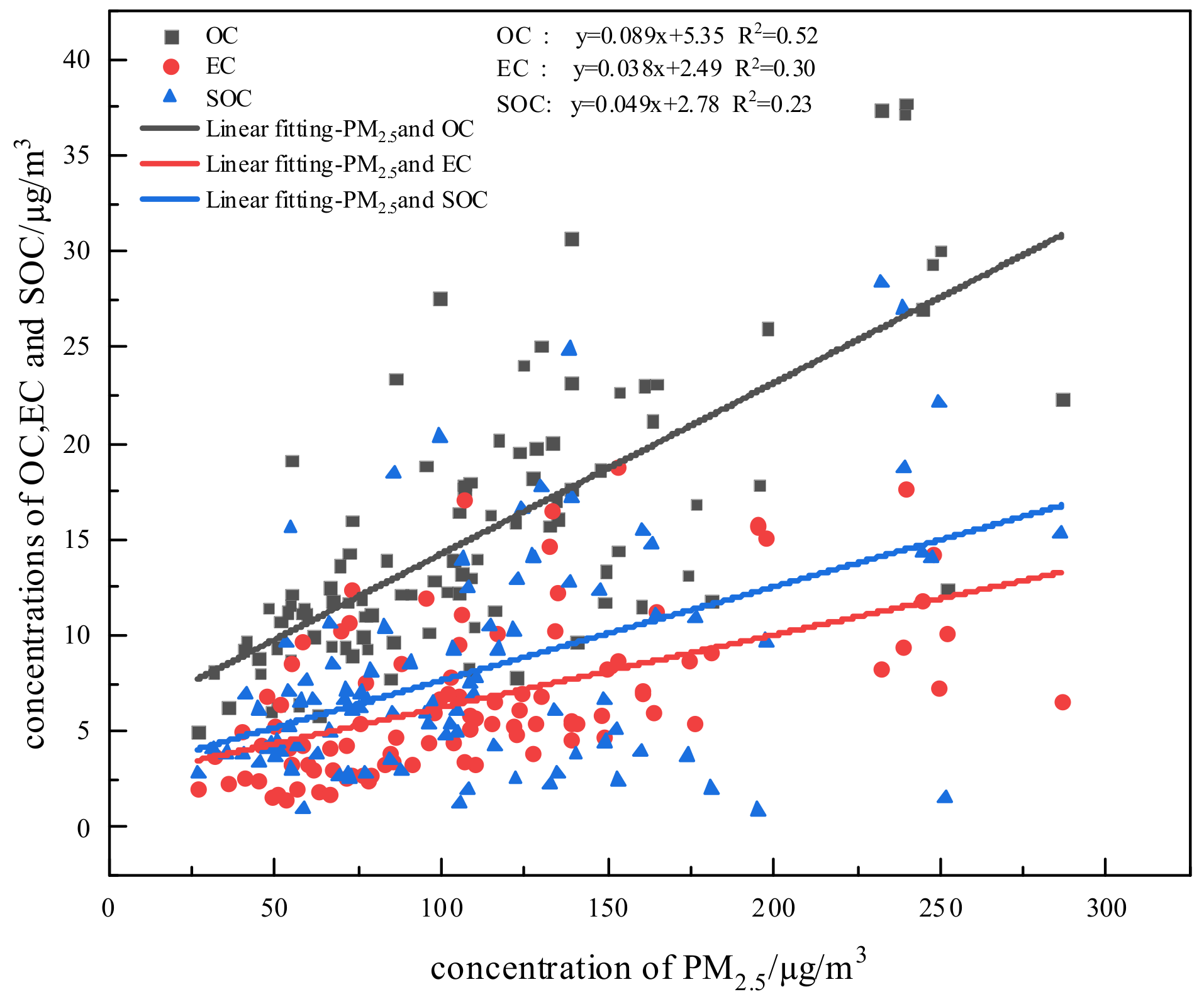
3.2.2. OC and EC Analysis

Carbonaceous species were found to contribute significantly to the formation of fine particles which mainly include EC and OC. EC is a good indicator of primary anthropogenic pollutants and it is one of the main light-absorbing species in fine particles. It is also the medium of gas-solid reaction for SO2 and NOx [51]. While the source of OC is more complex, besides the primary emissions from fuel combustion, industrial production and natural sources, there is secondary organic carbon (SOC) produced by photochemical reactions of gaseous precursors in the atmosphere. The mean concentrations of OC and EC were 15.20 ± 7.02 μg/m3 and 6.66 ± 3.95 μg/m3 in the autumn and winter in Liaocheng. The concentrations of OC and EC increased with the increase of pollution degree and reached 22.93 μg/m3 and 10.45 μg/m3 at SSD from 10.22 μg/m3 and 4.43 μg/m3 at CLD, respectively.
Usually, the OC/EC value is often used to judge a pollution source preliminarily. The relevant studies show that OC/EC between 1.0 and 4.2 indicates the presence of vehicle exhaust emissions [52]; OC/EC between 2.5 and 10.5 indicates the presence of coal-burning emissions [34] and OC/EC between 3.8 and 13.2 indicates the presence of biomass combustion emissions [53]. Chow [54] considered that when OC/EC exceeds 2, there is a secondary organic carbon presence. Through calculation, the average OC/EC value during the sample period was 2.28, therefore, secondary pollution more likely happened in the autumn and winter in Liaocheng, and the main source may be vehicle exhaust. Moreover, the concentrations of SOC could also reflect the level of secondary pollution and were also calculated. The concentration of SOC was 8.01 ± 5.95 μg/m3 and accounted for 52.7% in OC. As the pollution degree increased, the concentration of SOC increased gradually from 5.43 μg/m3 at CLD to 11.65 μg/m3 at SSD, but its proportion in OC decreased from 53.1% to 50.8%. The correlations between PM2.5 and OC, EC and SOC are shown in Figure 5. As seen in Figure 5, OC, EC and SOC were significantly correlated with PM2.5, and the R2 (Pearson coefficient) were 0.52, 0.30 and 0.23, respectively, suggesting that PM2.5 concentrations were affected by organic matter to some extent, but secondary organic pollution was not the main reason for the increase of PM2.5 concentrations.

3.2.3. Elemental Analysis

Elements were mainly divided into two groups: (1) crustal elements like Si, Ca, Mg, Al and Fe, which were considered as the main indicators of crustal dust; (2) anthropogenic elements including Mn, Ni, Cu, Zn, As, Se, Cd, Sb, Pb, et al., which probably originated from fossil fuel combustion, industrial metallurgical processes and vehicle emissions [55,56]. The total concentration of elements in the study was 12.21 ± 4.84 μg/m3 and accounted for 11.1% of PM2.5 mass. With increased pollution degree, the elements’ concentration increased from 11.81 μg/m3 at CCD to 12.6 μg/m3 at MMD, while the proportion in PM2.5 decreased significantly from 21.4% to 6.2%, which indicates that elements were not the cause of the PM2.5 concentration increase. The concentrations of element species follow the order of Si > Ca > Al > K > Fe > Na > Mg > Zn > Pb > Ti > Mn > Cu > Ba > Cr > As > Sn > Sb > Ni > V > Cd > Li > Co, and Si, Ca, Al, K and Fe were the abundant elements quite possibly coming from crustal dust with the average concentrations of 3.99 ± 2.03, 2.74 ± 1.37, 1.53 ± 0.79, 1.47 ± 0.60 and 1.10 ± 0.49 μg/m3, respectively. With the increase of pollution degree, the concentrations of Si, Ca, Mg and Ti gradually decreased, while the concentrations of other elements basically showed a gradually increasing trend, indicating that with the pollution increase, the natural sources of elements decreased, while the influence of anthropogenic source increased to some extent.

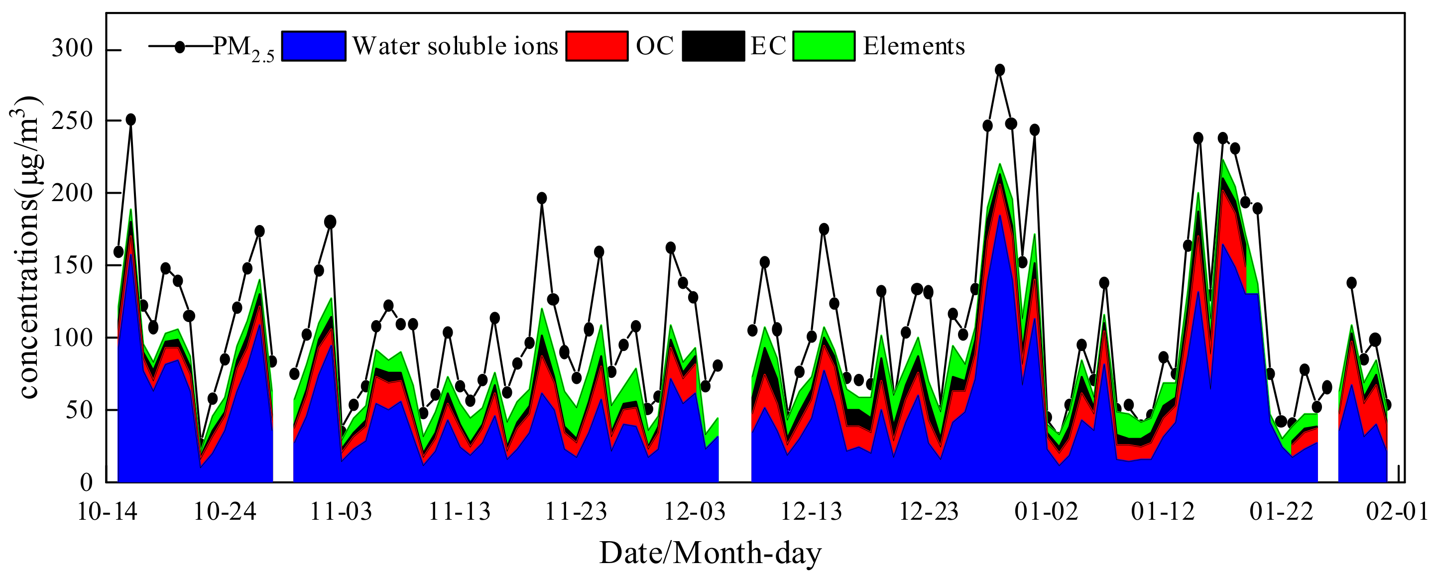
3.3. PM2.5 Mass Reconstruction

The results of PM2.5 mass reconstruction during CCD, MMD and SSD are shown in Figure 6, including SNA (sum of NO3, SO42− and NH4+), other soluble ions, organic matter (OM), EC, crustal matter (CM), other elements, and non-identified compositions. OM is estimated as OC multiplied by 1.6 for urban areas [57]. The sum of Na+, K+, F and Cl concentrations were calculated [58] as other soluble ions, and 20 concentrations of elements (all elements except Al, Si, Ca, Fe and Mg) as other elements. CM is calculated using the crustal species, which can be expressed as Equation (7). Additionally, there were some unknown components in the chemical mass reconstruction results which may come from the other components that cannot be measured, the mass weighing error of PM2.5, the measurement error of chemical components and the deviation of conversion coefficient; this part was defined as UD. After reconstruction, PM2.5 concentrations were significantly correlated with the monitored value, R and average residual were 0.96 and 0, respectively, indicating that the reconstructed data were effective, while the monitoring data and chemical composition analysis data were highly reliable, too.
CM = 2.20[Al] + 2.49[Si] + 1.63[Ca] + 2.42[Fe] + 1.93[Mg]
The reconstruction of PM2.5 during the sample period and different pollution degrees are shown in Figure 7. SNA, OM and CM were the main chemical components of PM2.5. As the pollution degree increased, the total chemical components’ concentrations increased significantly, as did SNA, and the concentrations were 13.97, 39.78, 99.48 μg/m3 and the proportions were 23.0%, 36.3%, 49.0% at CLD, MMD, SSD, respectively, while the ratio of SNA/PM2.5 at SSD was 6.17 times than that at CLD. SNA mainly came from secondary transformation of SO2, NOx and NH3. Coal combustion produces lots of pollutants in the autumn and winter in Liaocheng, while vehicle emissions and transit vehicles also have a certain amount of emission. Combined with the relatively stable weather conditions, pollutants were more likely to undergo secondary transformation under low temperature and high humidity conditions [59], resulting in a higher concentration and proportion of SNA. As for OM, the concentrations and proportions were 16.34, 24.72, 36.69 μg/m3 and 27.1%, 22.6%,18.1% at CLD, MMD and SSD, respectively. With the increase of pollution degree, the concentration increased but the proportion decreased, while the change trend of EC was similar with that of OM. The concentration and proportions of CM were 17.82, 17.59 and 16.36 μg/m3 at CLD, MMD and SSD, respectively. With the increase of pollution degree, CM concentration decreased slightly, but the proportions decreased significantly. The ratio decreased from 29.6% at CLD to 8.1% at SSD. CM is mainly derived from dust, which indicated that the contribution of dust may have obviously decreased with the increase of pollution degree. Generally, PM2.5 in autumn and winter in Liaocheng was dominated by SNA, OM and CM, and SNA was the main reason for the increase of PM2.5 concentrations, so the control of its precursors like SO2 and NOx was particularly important.

3.4. Source Apportionment of PM2.5

3.4.1. Source Apportionment of PM2.5 Using PMF

In this study, 26 species including PM2.5 were used as input data for the PMF model. In general, SOA and SOC data were removed from PM2.5 and OC, respectively, in order to reduce the SOC influence of the calculation. The factor number performed ranged from 1 to 7, and the five-factor with FPEAK = 0 solution was found to provide the “optimal solution”. Under this solution, residuals of the majority of standardized species were between −3 and +3, G-space plots showed data points lying within the source axes. The results of five source factors with clear profile and physical meaning are shown in Figure 8.
Factor 1 showed major loadings of POC, EC, As, Cd and K+. Both source profiles measured in the laboratory and the chemical analysis of ambient PM2.5 samples have indicated that OC and EC can be considered as tracer contents of coal combustion. K+ is primarily emitted from biomass burning [49], and As is often used as a marker for coal-fired power plant emissions [60], so Factor 1 has been identified as the combustion-related source.
Factor 2 was significantly loaded on SO42−, NO3 and NH4+ and could be identified as a mixture of secondary aerosols of nitrates and sulfates. In the atmosphere, the formation of secondary ions is mainly from gaseous precursors (SO2, NH3 and NOx) created by anthropogenic activities.
Factor 3 was predominantly loaded on Ni, Zn, Cr, V, Mn and Pb. It is generally believed that Zn, Mn, Cr and Ni are the indicator species of metallurgical emissions [61], and V is usually discharged by oil-fired power plants and steam boilers [62]. Therefore, Factor 3 was identified as the industrial process source related to metal processing.
Factor 4 showed high loadings for POC, EC, Zn, Pb, Mn, Cu and Ni. In general, EC is the characteristic element of vehicles [63], while vehicle brake wear, tire wear and oil drip could result in greater abundance of Zn, Mn and Pb in paved road dust [64]. Zn is also a marker element with Pb for transportation, because utilization of Pb as a fuel additive nowadays has been banned. Therefore, Factor 4 represents the pollution of vehicles.
Factor 5 was significantly loaded on Mg2+, Ca2+, Ti, Al and Si. Ions like Mg2+ and Ca2+ are often used to identify building dust, while Al, Si and Ti are mainly related to dust blown into the atmosphere by soil or rock weathering, so Factor 5 was identified as dust source.
The source of PM2.5 during the sampling period is shown in Figure 9, according to the result of PMF. It showed that secondary transformation had the most abundant contribution to PM2.5 (36.7%), followed by combustion-related source (20.4%). The contributions of SOA and mobile sources were not significantly different, accounting for 11.7% and 11%, respectively, while the contributions of dust sources and industrial process sources were 10.5% and 9.7%, respectively (Figure 8). Regarding different pollution degrees, at CLD dust sources contributed the most (22.7%), followed by mobile sources (19.2%) and combustion sources (17%), the contribution of SOA and industrial process sources were 15.7% and 14.9%, respectively, while secondary transformation was the lowest (10.4%). In the case of MMD, the contribution of secondary transformation sources increased significantly (31.4%), while the contribution of combustion sources also increased to a certain extent (23.5%), other sources’ contribution decreased with different ranges, especially dust and industrial process, which decreased to 11% and 11.2%, respectively. However, in the case of SSD, the proportion of secondary transformation increased sharply again, reaching 57%, more than five times that at CLD, while the contribution proportion of other pollution sources decreased to some extent. The contribution proportion of combustion sources decreased to 18%, and the contributions of other pollution sources were less than 10%. Generally, as the pollution degree increased, the contribution of secondary transformation increased significantly, that of combustion sources first increased and then decreased, while the contributions of dust sources, mobile sources, industrial process sources and SOA gradually decreased. In autumn and winter, the diffusion conditions were unfavorable when the pollution was heavy, the humidity was also relatively high and secondary transformation was conducive. Therefore, efforts should be made to control the emission of PM2.5 precursors including NOx and SO2, with the focus on coal burning and vehicle exhaust emissions, in order to reduce the generation of secondary inorganic particles.

3.4.2. Source Analysis of PM2.5 Using Back Trajectory and Clustering

Regional transport has important influence of the formation of air pollution. Thus, the transport of PM2.5 during the sample period was studied. The clustering analysis of the backward flow trajectory of the sampling period was conducted, and the result are shown in Figure 10. It showed that there were five transport paths during the sampling period. The short-distance transport from the northeast and west-northwest (cluster 1 and cluster 2) directions ratio were high, accounting for 29% and 28% of the total trajectory, respectively. The third type of trajectory from southeast to Liaocheng from Anhui Province was the shortest (cluster 3), accounting for 17% of the total trajectory. The fourth and fifth types of trajectories were relatively long, both from the northwest to Liaocheng via Inner Mongolia and Hebei Province, accounting for 15% (cluster 4) and 11% (cluster 5) of the total trajectories, respectively.
Source resolution results of atmospheric PM2.5 are classified according to air mass sources, which is helpful in determining the spatial orientation of atmospheric PM2.5 pollution sources. PM2.5 source resolution results corresponding to various trajectories are also shown in Figure 9. The contribution of secondary transformation of clusters 1, 2 and 3 which transmitted in short distance were relatively high, accounting for more than 40% of PM2.5 and suggesting that the accumulation of local pollutants was conducive to the secondary reaction when the weather was calm and stable. The secondary transformation proportions of cluster 4 and 5 transmitted by long distance were significantly lower, especially cluster 5, but the dust sources’ contributions of cluster 4 and 5 were significantly higher. Wind speed was higher during long distance transmission, so it more easily led surface dust pollution. There was little difference in the contribution of industrial sources of every cluster. The contribution of cluster 1 and cluster 3 was slightly higher, accounting for 12.1% and 12.5% respectively. Cluster 1 passed through Shandong Province, while cluster 3 was mainly influenced by cities of Anhui Province, which had more industrial enterprises. As for cluster 4 and cluster 5, mobile sources and SOA contributed more, which may be related to the route crossing Hebei. However, the contribution of combustion sources was the highest, which may be related to the primary pollutants and coal burning in winter in North China.

4. Conclusions

(1)
During the study period, the concentration of PM2.5 varied from 26.7 to 286.3 μg/m3, with an average concentration of 109.7 ± 56.8 μg/m3 in autumn and winter in Liaocheng, which was 0.46 times higher than the limit value of PM2.5 concentration CAAQS (GB 3095-2012) (daily standard: 75 μg/m3). Number of pollution days accounted for 67.6% of sampling period.
(2)
The concentration of water-soluble ions, OC, EC and elements were 50.47, 15.2, 6.66, 12.21 μg/m3 and accounted for 46.0%,13.9%,6.1% and 11.1% of PM2.5 concentrations, respectively. SNA were the main component of water-soluble ions and accounted for 84.7%, while the concentration of SOC was 8.01 μg/m3 and accounted for 52.7% of OC.
(3)
The concentrations of water-soluble ions, OC, EC and elements were 19.85, 10.22, 4.43, 11.81 μg/m3, 47.32, 15.45, 6.65 and 12.32 μg/m3, 110.29, 22.93, 10.45 and 12.60 μg/m3 at CLD, MMD and SSD, respectively. With the increase of pollution degree, the concentration of water-soluble ions and carbon components increased significantly, while the concentration of inorganic elements only increased slightly.
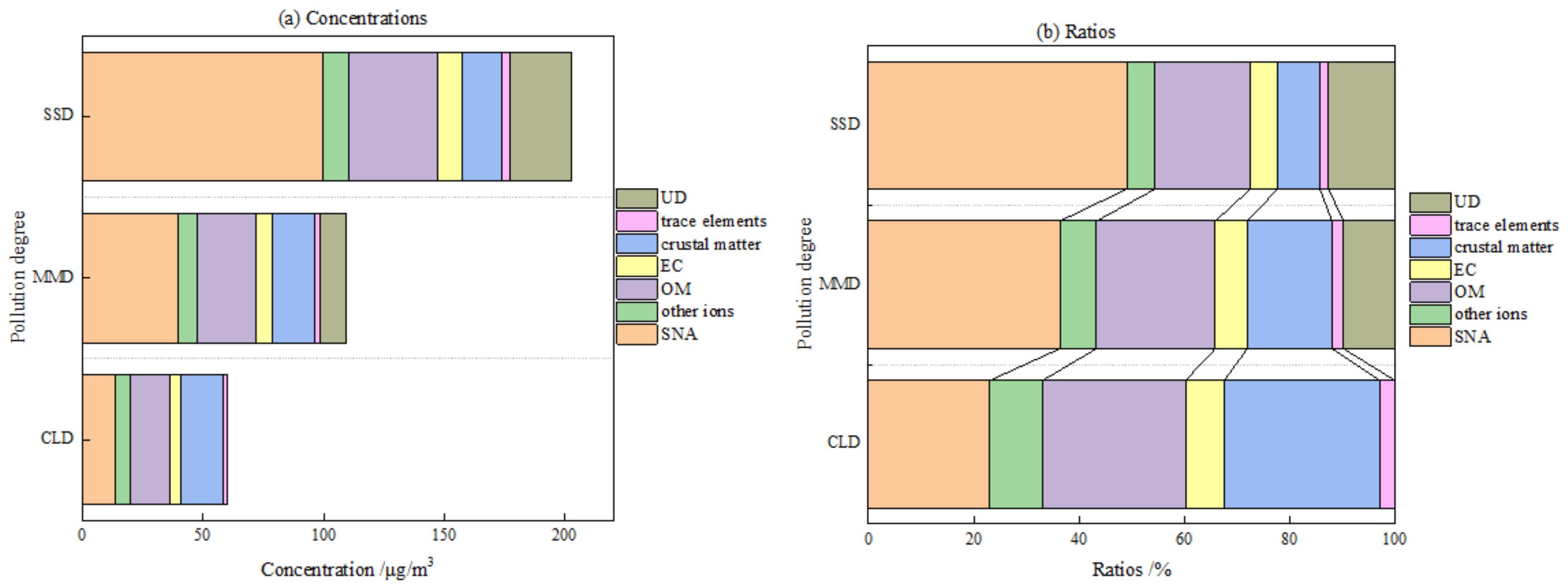
(4)
The results of chemical composition reconstruction showed that SNA and OM accounted for a higher proportion of PM2.5, which were 39.0% and 22.2%, respectively. The proportion of crustal substances, other ions, EC and trace elements were relatively low, 15.9%, 7.0%, 6.1% and 2.1%, respectively. The proportion of SNA increased significantly with the increase of pollution degree, from 23.0% at CLD to 49.0% at SSD. The proportion of other components decreased, especially crustal materials.
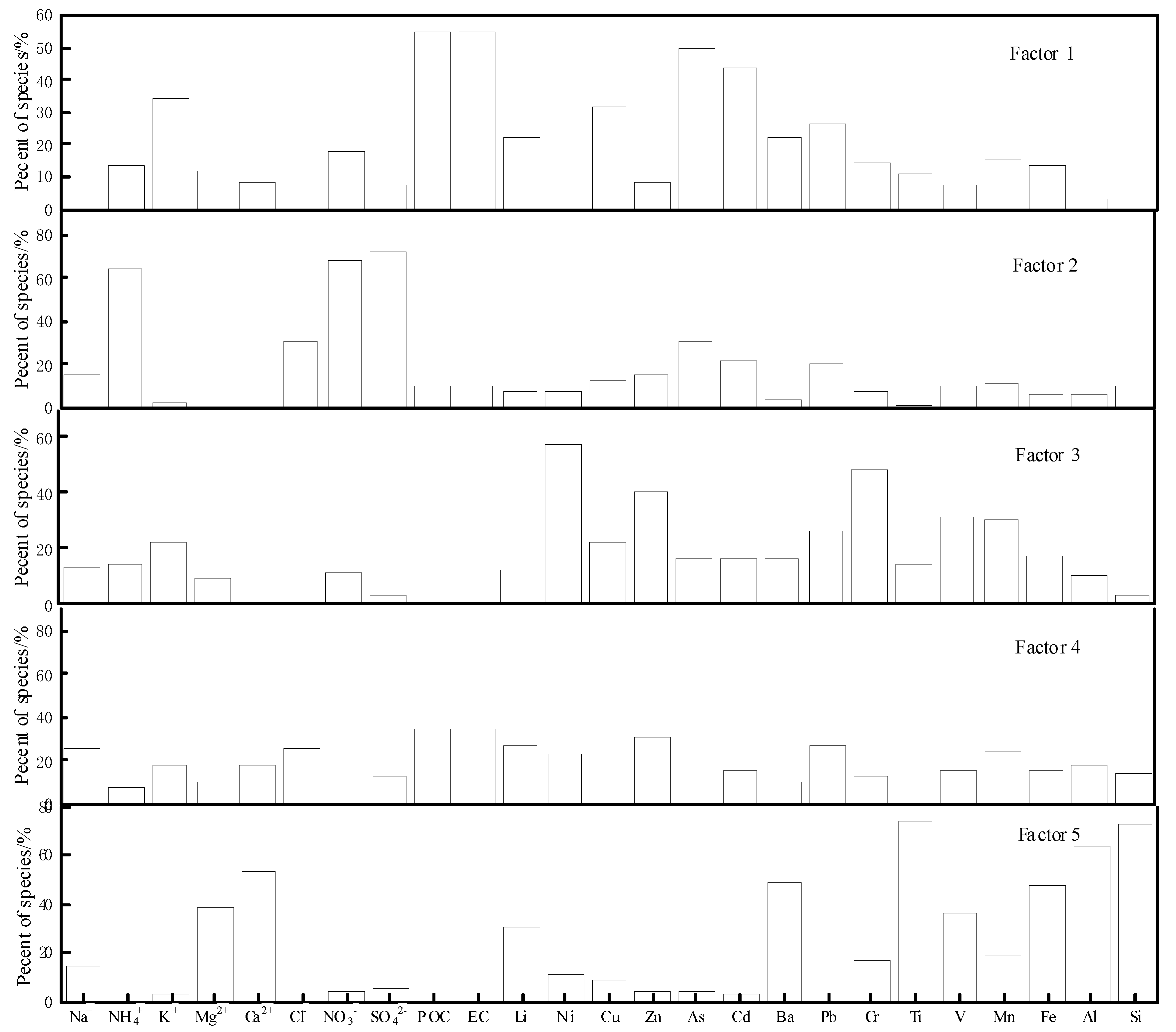
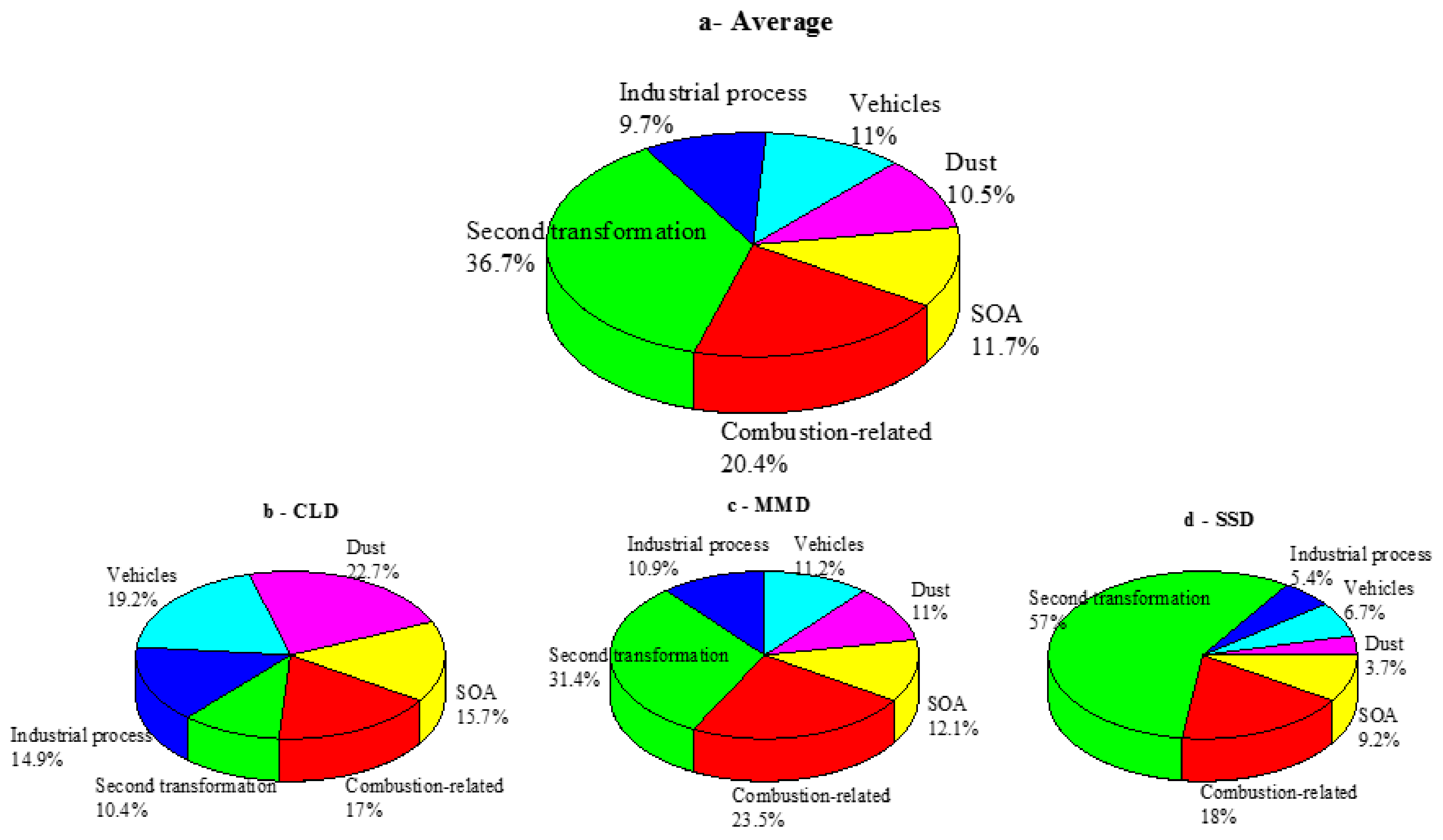
(5)
Five factors of PM2.5 have been identified by PMF: secondary transformation sources (36.7%), combustion-related sources (20.4%), SOA (11.7%), vehicle emissions (11%), dust (10.5%) and industrial processes (9.7%). The contribution of secondary inorganic sources, which was the main cause of the PM2.5 concentration rise, reached 57% in SSD.
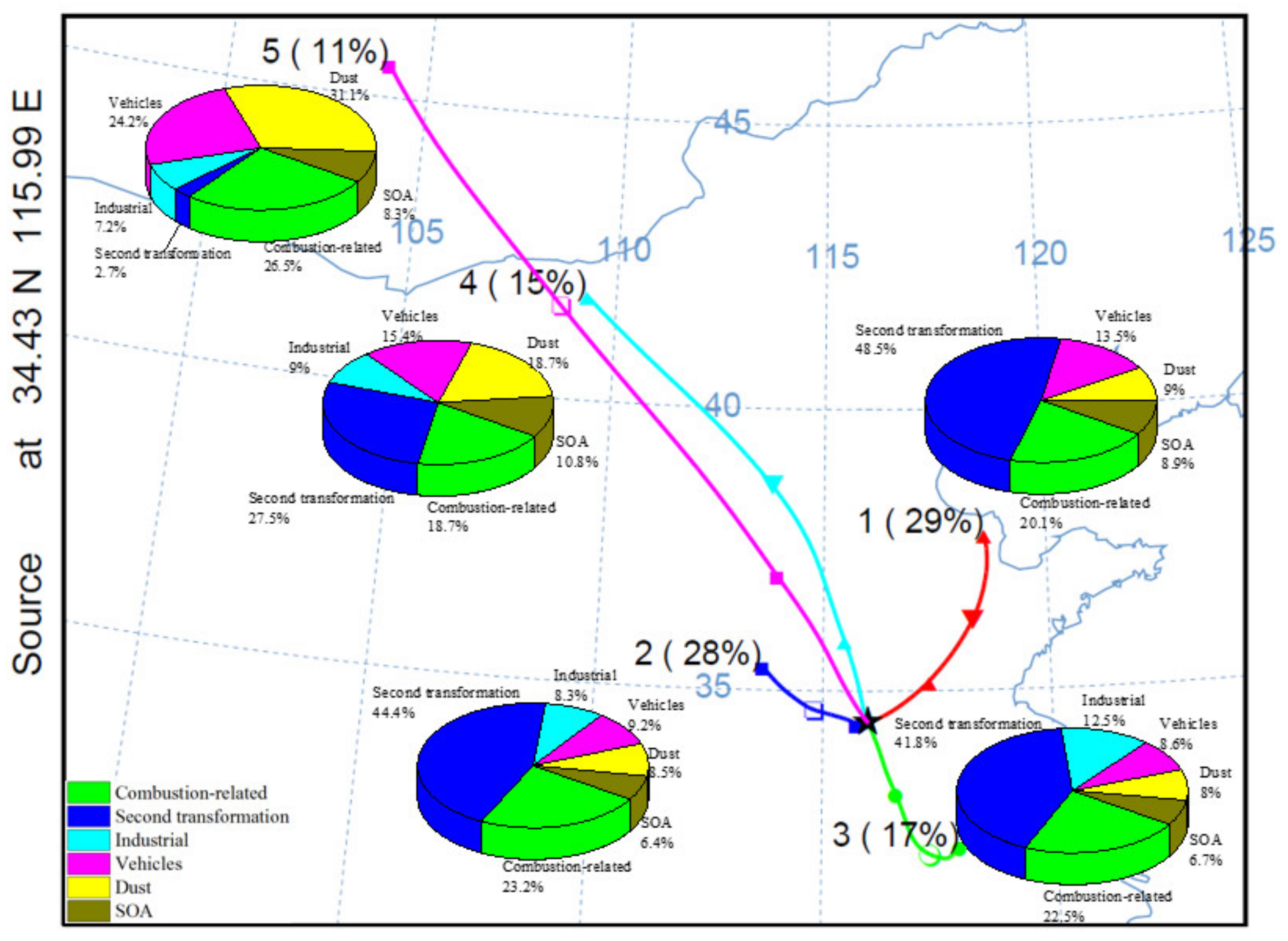
(6)
During the study period, the air mass mainly came from five paths in Liaocheng, and the air mass from the Shandong province and the northeast accounted for a higher proportion. The secondary transformation contribution of the air mass with short transmission distance like that in clusters 1, 2 and 3 were higher, while the contribution of the dust from the long distance, like clusters 4 and 5, were higher.

Author Contributions

Conceptualization, S.W. and H.W. (Hongliang Wang).; methodology, J.Z. and W.D.; data analysis and discussion of the results, L.Y. and R.L.; sample collection and data determination and validation, H.W. (Han Wang) and R.L.; writing—original draft preparation, J.Z.; writing—review and editing, J.Z., S.W. and H.W. (Han Wang). All authors have read and agreed to the published version of the manuscript.

Funding

This work was supported by National Research Program for Key Issues in Air Pollution Control, China (DQGG0107-21).

Institutional Review Board Statement

Not applicable.

Informed Consent Statement

Not applicable.

Data Availability Statement

Not applicable.

Acknowledgments

The authors would like to thank the Bureau of Ecology and Environment of Liaocheng for administrative support of this study and thank the Environmental Monitor Center of Liaocheng for technical support of this study.

Conflicts of Interest

The authors declare no conflict of interest.

References

  1. Circular of the State Council on Printing and Distributing the Action Plan for the Prevention and Control of Air Pollution. Available online: http://www.gov.cn/zwgk/2013-09/12/content_2486773.htm (accessed on 12 September 2013).
  2. Circular of the State Council on Printing and Distributing the Three-Year Action Plan for Winning the Battle against Blue Sky. Available online: http://www.gov.cn/zhengce/content/2018-07/03/content_5303158.htm (accessed on 27 June 2018).
  3. China Ecological and Environmental Status Bulletin. 2019. Available online: http://www.mee.gov.cn/hjzl/sthjzk/zghjzkgb/202006/P020200602509464172096.pdf (accessed on 2 June 2020).
  4. Dao, X.; Ji, D.S.; Zhang, X.; Zhang, X.; Tang, G.G.; Liu, Y.; Wang, L.L.; Cheng, L.J.; Wang, Y.S. Characteristics of chemical composition of PM2.5 in Beijing-Tianjin-Hebei and its surrounding areas during the heating period. Res. Environ. Sci. 2021, 34, 1–10. [Google Scholar]
  5. Li, L.; An, J.Y.; Zhou, M.; Qiao, L.P.; Zhu, S.H.; Yan, R.S.; Ooi, C.G.; Wang, H.L.; Huang, C.; Huang, L. An integrated source apportionment methodology and its application over the Yangtze River Delta region, China. Environ. Sci. Technol. 2018, 26, 14216–14227. [Google Scholar] [CrossRef] [PubMed]
  6. Yu, G.H.; Su, C.P.; Cao, L.M.; Wang, C.; Huang, X.F. Source apportionment of organic matter in atmospheric PM2.5 of a typical light-industrial zone in the Pearl River Delta. Environ. Sci. Technol. 2020, 43, 155–162. [Google Scholar]
  7. Wen, W.; He, X.D.; Ma, X.; Wei, P.; Cheng, S.Y.; Wang, X.Q.; Liu, L. Understanding the regional transport contributions of primary and secondary PM2.5 components over Beijing during a severe pollution episode. Aerosol Air Qual. Res. 2018, 18, 1720–1733. [Google Scholar] [CrossRef] [Green Version]
  8. Ding, J.; Zhang, Y.F.; Zhao, P.S.; Xiao, Z.M.; Zhang, W.H.; Zhang, H.T.; Yu, Z.J.; Du, X.; Li, L.W.; Yuan, J. Comparison of size-resolved hygroscopic growth factors of urban aerosol by different methods in Tianjin during a haze episode. Sci. Total. Environ. 2019, 678, 618–626. [Google Scholar] [CrossRef]
  9. Guan, Y.N.; Zhang, B.X.; Ni, S.Y.; Wang, H.H.; Lu, J.J.; Han, J.; Zhao, Y.G.; Duan, E.H.; Hou, L.A. Relationship between atmospheric visibility and particulate matter pollution in addition to relative humidity in Shijiazhuang. J. Saf. Environ. 2020, 20, 2001–2008. [Google Scholar]
  10. Wang, S.B.; Wang, H.; Zhang, J.Q.; Li, H.; Wu, Y.J.; Liu, R.Z.; Wang, S.L. Characterization analysis of PM2.5 and water-soluble ions during autumn in Xingtai City. China Environ. Sci. 2020, 40, 1877–1884. [Google Scholar]
  11. Yang, L.X.; Wang, D.C.; Cheng, S.H.; Wang, Z.; Zhou, Y.; Zhou, X.H.; Wang, W.X. Influence of meteorological conditions and particulate matter on visual range impairment in Jinan, China. Sci. Total. Environ. 2007, 383, 164–173. [Google Scholar] [CrossRef] [PubMed]
  12. Qiao, L.P.; Cai, J.; Wang, H.L.; Wang, W.B.; Zhou, M.; Lou, S.R.; Chen, R.J.; Dai, H.X.; Chen, C.H.; Kan, H.D. PM2.5 constituents and hospital emergency-room visits in Shanghai, China. Environ. Sci. Technol. 2014, 48, 10406–10414. [Google Scholar] [CrossRef]
  13. Guo, Z.Y.; Yang, Y.X.; Peng, L.; Lian, X.F.; Fu, Y.Z.; Zhang, G.H.; Bi, X.H.; Wang, X.M. The size-resolved light absorption contribution of water soluble organic carbon in the atmosphere of Guangzhou. China Environ. Sci. 2021, 41, 497–504. [Google Scholar]
  14. Liu, B.S.; Bi, X.H.; Feng, Y.C.; Dai, Q.L.; Xiao, Z.M.; Li, L.W.; Wu, J.H.; Yuan, J.; Zhang, Y.F. Fine carbonaceous aerosol characteristics at a megacity during the Chinese Spring Festival as given by OC EC online measurements. Atmos. Res. 2016, 181, 20–28. [Google Scholar] [CrossRef]
  15. Costa, D.L.; Dreher, K.L. Bioavailable transition metals in particulate matter mediate cardiopulmonary injury in healthy and compromised animal models. Environ. Health Perspect. 1997, 105, 1053–1060. [Google Scholar] [PubMed] [Green Version]
  16. Zhu, T.; Feng, Y.C. Atmospheric Particulate Matter Source Analysis; Science Press: Beijing, China, 2012; pp. 8–9. [Google Scholar]
  17. Zhang, J.Q.; Wu, Y.J.; Zhang, M.; Wang, H.; Chen, Z.X.; Hu, J.; Li, H.; Fan, X.L.; Chai, F.H.; Wang, S.L. PM2.5 pollution characterization and cause analysis of a winter heavy pollution event, Liaocheng city. Environ. Sci. 2018, 39, 4026–4033. [Google Scholar]
  18. Yi, Y.N.; Hou, Z.F.; Meng, J.J.; Yan, L.; Wang, X.P.; Liu, X.D.; Fu, M.X.; Wei, B.J. Diurnal variations and source analysis of water-soluble compounds in PM2.5 during the winter in Liaocheng city. Environ. Sci. 2019, 40, 4319–4329. [Google Scholar]
  19. Zhang, J.Q.; Luo, D.T.; Wang, S.B.; Wang, H.; Hu, W.Z.; Li, H.; Liu, R.Z.; Wang, S.L. Characterization and source analysis of PM2.5 and water-soluble ions during winter in Liaocheng city. Res. Environ. Sci. 2018, 31, 1712–1718. [Google Scholar]
  20. Charles, L.B.; Philip, M.R.; Shelley, J.T.; Steve, D.Z.; John, H.S. The use of ambient measurements to identify which precursor species limit aerosol nitrate formation. J. Air Waste Manag. Assoc. 2011, 50, 2073–2084. [Google Scholar]
  21. Ambient Air-Determination of the Water Soluble Anions (F, Cl, Br, NO2, NO3, PO43−, SO32−, SO42−) from Atmospheric Paticles-Ion Chromatography. Available online: http://www.mee.gov.cn/ywgz/fgbz/bz/bzwb/jcffbz/201605/t20160519_337906.shtml (accessed on 13 May 2016).
  22. Ambient Air-Determination of the Water Soluble Cations (Li+, Na+, NH4+, K+, Ca2+, Mg2+) from Atmospheric Particles-Ion Chromatography. Available online: http://www.mee.gov.cn/ywgz/fgbz/bz/bzwb/jcffbz/201605/t20160519_337907.shtml (accessed on 13 May 2016).
  23. Willeke, K.; Baron, P.A. Aerosol Measurement: Principles, Techniques and Applications; Van Nostrand Reinhold: New York, NY, USA, 1993; p. 249. [Google Scholar]
  24. Guide to Source Analysis and Monitoring of Ambient Air Particlate Matter. Available online: http://www.mee.gov.cn/xxgk2018/xxgk/sthjbsh/202005/W020200514318605389760.pdf (accessed on 1 May 2020).
  25. Chow, J.C.; Watson, J.G.; Pritchett, L.C.; Pierson, W.R.; Frazier, C.A.; Purcell, R.G. The dri thermal optical reflectance carbon analysis system–Description, evaluation and applications in United-States air-quality studies. Atmos. Environ. Part A Gen. Top. 1993, 27, 1185–1201. [Google Scholar] [CrossRef]
  26. Chow, J.C.; Watson, J.G.; Chen, L.W.A.; Paredes, M.G.; Chang, M.C.O.; Trimble, D.; Fung, K.K.; Zhang, H.; Zhen, Y.J. Refining temperature measures in thermal/optical carbon analysis. Atmos. Chem. Phys. 2005, 5, 2961–2972. [Google Scholar] [CrossRef] [Green Version]
  27. Chow, J.C.; Watson, J.G.; Chen, L.W.A.; Oliver, M.C.; Norman, F.C.; Dana, R.; Steven, K.t. The IMPROVE-A temperature protocol for thermal/optical carbon analysis: Maintaining consistency with a long-term database. J. Air Waste Manag. 2007, 57, 1014–1023. [Google Scholar] [CrossRef] [Green Version]
  28. Ambient Air and Waste Gas From Stationary Sources Emission-Determination of Metal Elements in Ambient Particle Matter-Inductively Coupled Plasma Optical Emission Spectrometry. Available online: http://www.mee.gov.cn/ywgz/fgbz/bz/bzwb/jcffbz/201512/t20151214_319107.shtml (accessed on 1 January 2016).
  29. Ambient Air and Stationary Source Emission-Determination of Metals in Ambient Particulat Matter Inductively Coupled Plasma/Mass Spectrometry(ICP-MS). Available online: http://www.mee.gov.cn/ywgz/fgbz/bz/bzwb/jcffbz/201308/t20130820_257714.shtml (accessed on 16 August 2013).
  30. Karthikeyan, S.; Balasubramanian, R. Inter laboratory study to improve the quality of trace element determinations in rainwater. Anal. Chim. Acta 2006, 576, 9–16. [Google Scholar] [CrossRef]
  31. Karthikeyan, S.; Joshi, U.M.; Balasubramanian, R. Rapid sample preparation using microwave for evaluation of bioavailability of trace elements in urban airborne particulate matter. Anal. Chim. Acta 2006, 576, 23–30. [Google Scholar] [CrossRef]
  32. Yao, X.H.; Chan, C.K.; Fang, M.; Cadle, S.; Chan, T.; Mulawa, P.; He, K.B.; Ye, B.M. The water-soluble ionic composition of PM2.5 in Shanghai and Beijing, China. Atmos. Environ. 2002, 4223–4234. [Google Scholar] [CrossRef]
  33. Zhang, Y.L.; Jun, L.; Gan, Z. Radiocarbon-based source apportionment of carbonaceous aerosols at a regional background site on Hainan Island, South China. Environ. Sci. Technol. 2014, 48, 2651–2659. [Google Scholar] [CrossRef]
  34. Chen, Y.; Zhi, G.; Feng, Y.; Fu, J.; Feng, J.; Sheng, G.; Simoneit, B.R.T. Measurements of emission factors for primary carbonaceous particles from residential raw-coal combustion in China. Geophys. Res. Lett. 2006, 33, 382–385. [Google Scholar] [CrossRef]
  35. Zheng, M.; Zhang, Y.J.; Yan, C.Q.; Zhu, X.L.; Schauer, J.J.; Zhang, Y.H. Review of PM2.5 source apportionment methods in China. Acta Sci. Nat. Univ. Pekin. 2014, 50, 1141–1154. [Google Scholar]
  36. US EPA. PMF 5.0 User Guide [EB/OL]. Available online: https://www.epa.gov/air-research/epa-positive-matrix-factorization-50-fundamentals-and-user-guide. (accessed on 10 April 2021).
  37. Zhao, Q.; Li, X.R.; Wang, G.X.; Zhang, L.; Yang, Y.; Liu, S.Q.; Sun, N.N.; Huang, Y.; Lei, W.K.; Liu, X.G. Chemical composition and source analysis of PM2.5 in Yuncheng, Shanxi province in autumn and winter. Environ. Sci. 2021, 42, 1626–1635. [Google Scholar]
  38. Wang, H.; Wang, S.L.; Zhang, J.Q.; Li, H. Characteristics of PM2.5 pollution with comparative analysis of O3 in Autumn–Winter Seasons of Xingtai, China. Atmosphere 2021, 12, 569. [Google Scholar] [CrossRef]
  39. Xu, R.; Zhang, H.D.; Yang, X.W.; Cheng, S.Y.; Zhang, T.H.; Jiang, Q. Concentration characteristics of PM2.5 and the causes of heavy air pollution events in Beijing during autumn and winter. Environ. Sci. 2019, 40, 3405–3414. [Google Scholar]
  40. Lei, T.Y.; Zhang, Y.; Gao, Y.G.; Li, G.; Wang, W.; Miao, Y.G.; Ren, L.H. Chemical characteristics of water-soluble ions of PM2.5 in autumn and winter in Heze city. Res. Environ. Sci. 2020, 33, 831–840. [Google Scholar]
  41. Chen, C.; Wang, T.J.; Li, Y.H.; Ma, H.L.; Chen, P.L.; Wang, D.Y.; Zhang, Y.X.; Qiao, Q.; Li, G.M.; Wang, W.H. Pollution characteristics and source apportionment of fine particulate matter in autumn and winter in Puyang, China. Environ. Sci. 2019, 40, 3421–3430. [Google Scholar]
  42. Miao, Q.Q.; Jiang, N.; Zhang, R.Q.; Zhao, X.N.; Qi, W.J. Characteristics and sources of PM2.5 pollutions in typical cities of the central plains Urban Agglomeration in autumn and winter. Environ. Sci. 2021, 42, 19–29. [Google Scholar]
  43. Liu, H.J.; Zhao, C.S.; Nekat, B.; Ma, N.; Wiedensohler, A.; Pinxteren, D.V.; Spindler, G.; Muller, K.; Herrmann, H. Aerosol hygroscopicity derived from size-segregated chemical composition and its parameterization in the North China Plain. Atmos. Chem. Phys. 2014, 14, 2525–2539. [Google Scholar] [CrossRef] [Green Version]
  44. Number of Motor Vehicles of Liaocheng City. 2016. Available online: http://www.liaocheng.gov.cn/xxgk/szfbmxxgk/sgaj/201901/t20190121_1913323.html (accessed on 17 February 2017).
  45. Conference of Etc Promotion and Application. Available online: http://jtj.liaocheng.gov.cn/xwzx_13663/jtyw/201908/t20190812_2345636.html (accessed on 12 August 2019).
  46. The Number of Private Cars Surpassed 200 Million for the First Time in 66 Cities, China. Available online: https://www.mps.gov.cn/n7944517/n7944597/n7945888/c7478950/content.html (accessed on 8 January 2020).
  47. Naoki, K.; Hiroshi, Y.; Tateki, M.; Kazuhiko, S.; Mastaka, S. Chemical forms and sources of extremely high nitrate and chloride in winter aerosol pollution in the Kanto Plain of Japan. Atmos. Environ. 1999, 33, 1745–1756. [Google Scholar]
  48. Zong, Z.; Wang, X.P.; Tian, C.G.; Chen, Y.J.; Qu, L.; Ji, L.; Zhi, G.R.; Li, J.; Zhang, G. Source apportionment of PM2.5 at a regional background site in North China using PMF linked with radiocarbon analysis: Insight into the contribution of biomass burning. Atmos. Chem. Phys. 2016, 16, 11249–11265. [Google Scholar] [CrossRef] [Green Version]
  49. Andreae, M.O. Soot carbon and excess fine potassium: Long-range transport of combustion-derived aerosols. Science 1983, 220, 1148–1151. [Google Scholar] [CrossRef] [PubMed]
  50. Lestari, P.; Mauliadi, Y.D. Source apportionment of particulate matter at urban mixed site in Indonesia using PMF. Atmos. Environ. 2009, 43, 1760–1770. [Google Scholar] [CrossRef]
  51. Pachauri, T.; Singla, V.; Satsangi, A.; Lakhani, A.; Maharaj, K.K. Characterization of carbonaceous aerosols with special reference to episodic events at Agra, India. Atmos. Res. 2013, 128, 98–110. [Google Scholar] [CrossRef]
  52. Schauer, J.J.; Kleeman, M.J.; Cass, G.R.; Simoneit, B.R.T. Measurement of emissions from air pollution sources.2.C1 through C30 organic compounds from medium duty diesel trucks. Environ. Sci. Technol. 1999, 33, 1578–1587. [Google Scholar] [CrossRef]
  53. Schauer, J.J.; Kleeman, M.J.; Cass, G.R.; Simoneit, B.R.T. Measurement of emissions from air pollution sources: 3.C1-C29 organic compounds from fireplace combustion of wood. Environ. Sci. Technol. 2001, 35, 1716–1728. [Google Scholar] [CrossRef]
  54. Chow, J.C.; Watson, J.G.; Lu, Z.Q.; Lowenthal, D.H.; Frazier, C.A.; Solomon, P.A.; Thuillier, R.H.; Magliano, K. Descriptive analysis of PM2.5 and PM10 at regionally representative locations during Sjvaqs/Auspex. Atmos. Environ. 1996, 30, 2079–2112. [Google Scholar] [CrossRef]
  55. Gao, J.J.; Tian, H.Z.; Cheng, K.; Lu, L.; Zheng, M.; Wang, S.X.; Hao, J.M.; Wang, K.; Hua, S.B.; Zhu, C.Y. The variation of chemical characteristics of PM2.5 and PM10 and formation causes during two haze pollution events in urban Beijing, China. Atmos. Environ. 2015, 107, 1–8. [Google Scholar] [CrossRef]
  56. Zhang, F.; Wang, Z.W.; Cheng, H.R.; Lv, X.P.; Gong, W.; Wang, X.M.; Zhang, G. Seasonal variations and chemical characteristics of PM2.5 in Wuhan, central China. Sci. Total Environ. 2015, 518, 97–105. [Google Scholar] [CrossRef] [PubMed]
  57. Xing, L.; Fu, T.M.; Cao, J.J.; Lee, S.C.; Wang, G.H.; Ho, K.F.; Cheng, M.C.; You, C.F.; Wang, T.J. Seasonal and spatial variability of the OM/OC mass ratios and high regional correlation between oxalic acid and zinc in Chinese urban organic aerosols. Atmos. Chem. Phys. 2013, 13, 4307–4318. [Google Scholar] [CrossRef] [Green Version]
  58. Yang, F.M.; He, K.B.; Ma, Y.L.; Zhang, Q.; Cadle, S.H.; Chan, T.; Mulawa, P.A. Characterization of mass balance of PM2.5 chemical speciation in Beijing. Environ. Chem. 2004, 23, 326–333. [Google Scholar]
  59. Tursic, J.; Berner, A.; Podkrajsek, B.; Grgic, I. Influence of ammonia on sulfate formation under haze conditions. Atmos. Environ. 2004, 38, 2789–2795. [Google Scholar] [CrossRef]
  60. Tian, H.Z.; Wang, Y.; Xue, Z.G.; Cheng, K.; Qu, Y.P.; Chai, F.H.; Hao, J.M. Trend and characteristics of atmospheric emissions of Hg, As and Se from coal combustion in China,1980–2007. Atmos. Chem. Phys. 2010, 10, 11905–11919. [Google Scholar] [CrossRef] [Green Version]
  61. Tao, J.; Gao, J.; Zhang, L.M.; Zhang, R.J.; Che, H.Z.; Zhang, Z.S.; Lin, Z.; Jing, J.; Cao, J.J.; Hsu, S.C. PM2.5 pollutions in a megacity of southwest China: Source apportionment and implication. Atmos. Chem. Phys. 2014, 14, 8679–8699. [Google Scholar] [CrossRef] [Green Version]
  62. Duan, J.C.; Tan, J.H. Atmospheric heavy metals and Arsenic in China: Situation, sources and control policies. Atmos. Environ. 2014, 74, 93–101. [Google Scholar] [CrossRef]
  63. Watson, J.G.; Chow, J.C.; Houck, J.E. PM2.5 chemical source profiles for vehicle exhaust, vegetative burning, geological material, and coal burning in Northwestern Colorado during 1995. Chemosphere 2001, 43, 1141–1151. [Google Scholar] [CrossRef]
  64. Yu, L.D.; Wang, G.F.; Zhang, R.J.; Zhang, L.M.; Song, Y.; Wu, B.B.; Li, X.F.; An, K.; Chu, J.H. Characterization and source apportionment of PM2.5 in an urban environment in Beijing. Aerosol Air Qual. Res. 2013, 13, 574–583. [Google Scholar] [CrossRef] [Green Version]
Figure 1. Sampling site location.
Atmosphere 12 01180 g001
Figure 2. PM2.5 mass concentration variation during the sampling period in Liaocheng.
Atmosphere 12 01180 g002
Figure 3. Concentration of chemical components of PM2.5 during the sampling period in Liaocheng.
Atmosphere 12 01180 g003
Figure 4. Correlation between temperature and relative humility with SOR/NOR.
Atmosphere 12 01180 g004
Figure 5. Correlation between PM2.5 with OC, EC and SOC.
Atmosphere 12 01180 g005
Figure 6. Standard P-P plots of regression normalized residuals.
Atmosphere 12 01180 g006
Figure 7. Reconstruction results of PM2.5 with different pollution levels during the sampling period.
Atmosphere 12 01180 g007
Figure 8. Source analysis of PM2.5 in autumn and winter in Liaocheng.
Atmosphere 12 01180 g008
Figure 9. Sources proportion of different pollution levels to PM2.5 in autumn and winter in Liaocheng.
Atmosphere 12 01180 g009
Figure 10. The clustering results and sources proportion of the different passes.
Atmosphere 12 01180 g010
Table 1. Meteorological parameters and PM2.5 concentrations at different pollution levels during the sampling period.
AverageCLDMMDSSD
Wind speed/m/s1.37 ± 0.411.44 ± 0.401.35 ± 0.411.33 ± 0.45
Temperature/°C5.80 ± 6.223.96 ± 5.316.91 ± 6.756.00 ± 5.76
RH/%44.15 ± 15.8538.38 ± 14.5744.19 ± 15.6553.56 ± 14.42
Air pressure/Pa1020.9 ± 5.11022.6 ± 5.21020.2 ± 5.21019.9 ± 4.2
Table 2. Concentration of chemical components of PM2.5 of different pollution degrees during the sampling period.
ComponentsAverage ConcentrationCLDMMDSSD
μg/m3
PM2.5109.7 ± 56.855.2 ± 12.3109.5 ± 21.8202.8 ± 41.5
water soluble ionsNa+0.41 ± 0.180.34 ± 0.100.40 ± 0.180.56 ± 0.19
NH4+9.40 ± 7.653.29 ± 1.599.03 ± 3.7820.73 ± 8.70
K+1.11 ± 0.460.78 ± 0.291.22 ± 0.391.40 ± 0.52
Mg2+0.14 ± 0.060.14 ± 0.060.15 ± 0.070.13 ± 0.07
Ca2+2.10 ± 1.122.20 ± 1.102.13 ± 1.151.83 ± 1.10
F0.11 ± 0.080.10 ± 0.070.11 ± 0.090.11 ± 0.10
Cl3.85 ± 2.582.46 ± 1.063.59 ± 1.966.87 ± 3.33
NO322.40 ± 19.446.64 ± 3.3421.47 ± 10.7551.56 ± 20.08
SO42−10.96 ± 10.883.93 ± 1.909.28 ± 5.2027.19 ± 14.05
SUM-IC50.42 ± 37.9119.85 ± 6.1147.32 ± 17.24110.29 ± 39.32
carbonOC15.20 ± 7.0210.22 ± 3.0615.45 ± 5.2322.93 ± 8.64
EC6.66 ± 3.954.43 ± 2.946.65 ± 3.3910.45 ± 4.04
SOC8.01 ± 5.955.43 ± 2.888.28 ± 5.5611.65 ± 8.47
ElementsLi0.0019 ± 0.00080.0015 ± 0.00060.0019 ± 0.00070.0026 ± 0.0010
Co0.0005 ± 0.00030.0004 ± 0.00020.0005 ± 0.00030.0005 ± 0.0003
Ni0.0057 ± 0.00480.0049 ± 0.00330.0064 ± 0.00620.0054 ± 0.0020
Cu0.0455 ± 0.02010.0338 ± 0.01570.0482 ± 0.01900.0587 ± 0.0199
Zn0.2016 ± 0.09140.1779 ± 0.10830.1955 ± 0.07990.2572 ± 0.0647
As0.0094 ± 0.00670.0041 ± 0.00210.0100 ± 0.00590.0171 ± 0.0054
Cd0.0025 ± 0.00170.0011 ± 0.00050.0028 ± 0.00160.0039 ± 0.0016
Sn0.0065 ± 0.00360.0044 ± 0.00300.0070 ± 0.00370.0090 ± 0.0025
Sb0.0060 ± 0.00340.0038 ± 0.00310.0060 ± 0.00260.0096 ± 0.0028
Ba0.0202 ± 0.00910.0181 ± 0.00850.0211 ± 0.00820.0214 ± 0.0117
Pb0.0734 ± 0.04000.0443 ± 0.02200.0753 ± 0.03360.1177 ± 0.0367
Na0.5020 ± 0.23010.4332 ± 0.17280.4861 ± 0.24480.6594 ± 0.2122
K1.4711 ± 0.60470.9903 ± 0.31681.5093 ± 0.41832.1913 ± 0.6347
Cr0.0102 ± 0.00550.0079 ± 0.00380.0109 ± 0.00560.0124 ± 0.0064
Ti0.0728 ± 0.04030.0775 ± 0.03830.0723 ± 0.04220.0657 ± 0.0395
V0.0030 ± 0.00140.0024 ± 0.00090.0031 ± 0.00140.0039 ± 0.0016
Mn0.0608 ± 0.02430.0496 ± 0.01950.0622 ± 0.02490.0764 ± 0.0212
Fe1.1028 ± 0.48681.0034 ± 0.46051.1247 ± 0.48381.2161 ± 0.5298
Mg0.3494 ± 0.18350.3693 ± 0.17440.3488 ± 0.18840.3172 ± 0.1904
Ca2.7409 ± 1.37012.9749 ± 1.29222.7356 ± 1.39172.3566 ± 1.4228
Al1.5279 ± 0.79001.5258 ± 0.65561.5946 ± 0.91021.3611 ± 0.6694
Si3.9964 ± 2.03544.0806 ± 1.94604.0023 ± 2.10813.8380 ± 2.0894
SUM12.21 ± 4.8411.81 ± 4.4712.32 ± 5.0512.60 ± 5.11
Publisher’s Note: MDPI stays neutral with regard to jurisdictional claims in published maps and institutional affiliations.

