Diagnostic Relations between Pressure and Entropy Perturbations for Acoustic and Entropy Modes

Abstract

Diagnostics and decomposition of atmospheric disturbances in a planar flow are considered and applied to numerical modelling with the direct possibility to use in atmosphere monitoring especially in such strong events which follow magnetic storms and other large scale atmospheric phenomena. The study examines a situation in which the stationary equilibrium temperature of a gas may depend on a vertical coordinate, which essentially complicates the diagnostics. The relations connecting perturbations for acoustic and entropy (stationary) modes are analytically established and led to the solvable diagnostic equations. These equations specify acoustic and entropy modes in an arbitrary stratified gas under the condition of stability. The diagnostic relations are independent of time and specify the acoustic and the entropy modes. They provide the ability to decompose the total vector of perturbations into acoustic and non-acoustic (entropy) parts uniquely at any instant within the total accessible heights range. As a prospective model, we consider the diagnostics at the height interval 120–180 km, where the equilibrium temperature of a gas depends linearly on the vertical coordinate. For such a heights range it is possible to proceed with analytical expressions for pressure and entropy perturbations of gas variables. Individual profiles of acoustic and entropy parts for some data are illustrated by the plots for the pure numerical data against those obtained by the model. The total energy of a flow is determined for both approaches and its vertical profiles are compared.

1. Introduction

Theoretical and numerical models which describe dynamics of gases and liquids affected by external forces are of great interest in geophysics, meteorology, and wave theory [1,2,3,4,5,6]. The external forces and sources of energy, as well as momentum transfer, make the background of a fluid non-uniform. Hence, equilibrium thermodynamic parameters should depend on spatial coordinates. This drastically complicates the definition of linear modes (motions of infinitely small magnitude) taking place in such non-uniform media, so-called “non-exponential”. The number of roots of the dispersion equation, if it is possible to determine them, agrees with the number of types of motion, and equals the number of balance equations [4]. Each of the balance equations represents a partial differential equation (PDE) which contains the first-order derivative with respect to time. In the case of isothermal gas in equilibrium with pressure and density depending exponentially on the coordinate (named often the “exponential atmosphere”), and in the simplest case of a planar flow, the dispersion relations may be introduced over the total wavelength range. This model is widely used for the classification of wave modes in practice as a “zero approximation”. The realistic non-exponential case needs either consideration of the atmosphere as a layered medium or, for the short waves, making use of the Wentzel, Kramers, Brillouin (WKB) method [3]. Generally, the sources like tsunami, lying at the lower boundary in the atmosphere usually excite combined waves with the leading front formed by quasi-planar acoustics [7].

There are three types of motion in a one-dimensional (1D) exponential atmosphere: two acoustic modes of different direction of propagation, and the entropy mode, corresponding to zero frequency in a linear lossless flow [1,2]. The entropy mode, however, is not stationary in a viscous fluid that conducts heat, and with a non-linearity account [1,4,8]. In the flows exceeding one dimension, the buoyancy, or “internal” waves appear [3,4]. For the Rossby and Poincare waves description see, e.g., [4,6]. The first results that allow distinguishing modes due to relations of specific perturbations have been obtained namely relative to the motion of an exponentially stratified ideal gas in the constant gravity field [6,8,9]. Mathematically, these relations are determined by the eigenvectors of the evolution operator which specifies the basic balance system.

Experimental observation of wave and non-wave disturbances is not easy, there are special facilities as “Sura” [10] based on the active experiment of ionosphere excitation that allows measuring directly the atmosphere parameters variations at the ionosphere heights [11]. Only recently an attempt to apply the diagnostic method, based on projecting operators technique, was realized within a set of such measurements. The projecting technique was developed for a space-evolution operator. That makes it possible to apply it to the relations of atmospheric parameters at a vicinity of a point of observation. It allowed to distinguish up- and down- directed acoustic wave via the real dataset [12] (in this paper the algorithm of entropy mode diagnosis was elaborated, see also [13]).

This work considers the dynamics of ideal atmosphere gas perturbations over a background of equilibrium temperature, dependent on height, affected by a gravity field and other geophysical impacts, for instance, geomagnetic storms. The main aim of this study is the diagnostics as decomposition of a total disturbance into wave and non-wave modes in the case of arbitrary stable stratification. This is helpful in the interpretation of experimental data related to the significantly disturbed atmosphere (e.g., by storms), it also may be useful in a validation of a numerical modelling [14]. Especially, it is important in establishing the location of wave sources, and modelling the atmosphere’s warming [15,16], related to the atmosphere gas wave heating. The theory should base on the balance equations and rely upon physically justified boundary conditions and simplifications [17], and the modes decomposition should be instructive in a specific mathematical statement of problem formulation [18,19].

In this study, which develops ideas of [20], the modes of a planar flow are determined by means of relations between specific perturbations that are time-independent. We name such relations as “diagnostic relations”. They are valid for arbitrary dependence of the equilibrium temperature on a coordinate for the case of a stable atmosphere. These relations give the ability to distinguish modes from the total field analytically at any instant, solving the diagnostic equations, that are the direct corollary of the mentioned diagnostic relations. That serves as a tool to predict their dynamics, and to conclude about the energy of modes (which remains constant in time). This is undoubtedly important in applications in meteorology and diagnostics of atmospheric dynamics, including the understanding of such phenomena as variations of the equilibrium temperature of the stratosphere, e.g., so-called warming [21] conventionally understood as period-average. Such phenomenon, also named “heating”, may be explained in the framework of non-linear interaction of acoustic wave and entropy modes in the presence of dissipation [16,22]. The whole exposition is also important in the diagnostics of wave and non-wave modes in order to follow experimental observations and numerical simulations [14] as an element of monitoring of atmospheric dynamics [23]. The authors of [23] stress, that the acoustic component of a perturbation is the first that reach ionosphere heights. This is important for the mentioned hazard phenomena detection.

As the practical example of the general theory and the particular model applications we use the dataset of numerical modelling of an atmospheric perturbation by the source, positioned at the vicinity of Earth surface [17,18]. The theory uses the standard atmosphere $H\left(z\right)$ profile [24] at the $z\in$$[0,500]$ km range with the application of diagnostic equations solution with the right-hand-side (RHS), discretized as the dataset from a numerical experiment we use. We should refer only to cases with non-negative energy density to avoid the instability of disturbances. For this aim, we choose a diagnostic at the interval at which the $H\left(z\right)$ profile is well approximated by a linear function. It is the heights range $z\in [120,180]$ km, for which we elaborate the model with the explicit form of the diagnostic equation solution. In the frames of this interval, we compare the results of the general theory digitization and the result of a more compact model, based on explicit approximation of the $H\left(z\right)$ profile at the pointed height range.

We begin from the basic system of the balance equations and derive the diagnostic ones (Section 2). In the final subsection, we solve the differential diagnostic equation by the method of factorization. Next, we apply the obtained relation to the datasets, obtained by numerical solution of an atmosphere perturbation problem [17] within the heights range $z\in$$[120,180]$ km, using the $H\left(z\right)$ profile from standard atmosphere [24]. It results in entropy mode contribution profiles (Section 5). In the Section 5.2 we build the model for the mentioned heights interval repeating the calculations, when possible, analytically, see also [25]. The results, obtained by the direct application of the theory to the dataset basing on the standard atmosphere within the range of approximate linear profile, and the conclusions of a model are compared.

2. Diagnostic Relations

2.1. Basic Balance Equations for Arbitrary Stable Stratification

The case of the non-exponential atmosphere in equilibrium permits to fix the entropy and acoustic mode without subdivision into “upwards” and “downwards” directed acoustic waves [20], see also [9]. The main functional parameter in this case, the local atmosphere’s scale height $H\left(z\right)$ depends on height as, e.g., in [24]. The background density which supports the equilibrium distribution of temperature $\overline{T}\left(z\right)$, takes the form:

$$\overline{\rho }\left(z\right)=\frac{\overline{\rho }\left(0\right)H\left(0\right)}{H\left(z\right)}exp\left(-{\int }_0^z\frac{d{z}^{\prime }}{H\left(z^{\prime }\right)}\right),$$

(1)

where the pressure scale height is

$$H\left(z\right)=\frac{\overline{p}}{\overline{\rho }g}=\frac{\overline{T}\left(z\right)(C_p-C_v)}{g}.$$

(2)

Here the conventional gas parameters are used: g-gravity acceleration, $C_{p,v}$ are the molar heat capacities at constant pressure and volume correspondingly. It is convenient to introduce the quantity ${\phi }^{\prime }$ instead of perturbation in density ${\rho }^{\prime }$

$${\phi }^{\prime }=p^{\prime }-\gamma \frac{\overline{p}}{\overline{\rho }}{\rho }^{\prime },$$

(3)

where the parameter $\gamma =C_p/C_v$. We will name it the entropy perturbation, because in the limit $g=0$ and constant background temperature $\overline{T}$, ${\phi }^{\prime }$ is responsible for the deviation of an ideal gas entropy from the equilibrium one [26,27].

As it was done in [25] we use the conventional set of variables:

$$P=p^{\prime }·exp\left(\underset{0}{\overset{z}{\int }}\frac{d{z}^{\prime }}{2H\left(z^{\prime }\right)}\right),$$

(4)

$$\mathsf{\Phi }={\phi }^{\prime }·exp\left(\underset{0}{\overset{z}{\int }}\frac{d{z}^{\prime }}{2H\left(z^{\prime }\right)}\right),$$

(5)

$$U=V·exp\left(-\underset{0}{\overset{z}{\int }}\frac{d{z}^{\prime }}{2H\left(z^{\prime }\right)}\right),$$

(6)

where $P,\mathsf{\Phi },U$ are the new quantities which represent the pressure perturbation $p^{\prime }$, entropy perturbation ${\phi }^{\prime }$ and the vertical velocity of the flow V correspondingly. The system of momentum-energy-mass balance equations in the new variables reads (see [9,25]):

$$\frac{\partial U}{\partial t}=\frac{1}{\overline{\rho }\left(0\right)}\left(\frac{\gamma -2}{2\gamma H\left(0\right)}-\frac{H\left(z\right)}{H\left(0\right)}\frac{\partial }{\partial z}\right)P+\frac{\mathsf{\Phi }}{\gamma H\left(0\right)\overline{\rho }\left(0\right)},$$

(7)

$$\frac{\partial P}{\partial t}=-\gamma gH\left(0\right)\overline{\rho }\left(0\right)\frac{\partial U}{\partial z}-gH\left(0\right)\overline{\rho }\left(0\right)\frac{\gamma -2}{2H\left(z\right)}U,$$

(8)

$$\frac{\partial \mathsf{\Phi }}{\partial t}=-\frac{\nu \left(z\right)}{H\left(z\right)}gH\left(0\right)\overline{\rho }\left(0\right)U,$$

(9)

where $\nu \left(z\right)$ is positive:

$$\nu \left(z\right)=\gamma -1+\gamma \frac{dH\left(z\right)}{dz}>0,$$

(10)

this guarantees the positive definition of energy, defined at the Section 6.

The system (7)–(9) is the initial problem which imposes the setting of unknown functions at $t=0$ as functions of z (see [28]).

2.2. Relation between Pressure and Entropy Perturbations for Acoustic and Entropy Modes

The relation between pressure and entropy perturbations within the acoustic mode, for arbitrary stable stratification of 1D atmosphere can be obtained by substituting Equation (9) into Equation (8) [25]. As a result, the diagnostic relation between the pressure and entropy perturbations within the acoustic mode follows:

$$P_a=\left(\frac{\gamma -2}{2\nu \left(z\right)}+\gamma \frac{\partial }{\partial z}\frac{H\left(z\right)}{\nu \left(z\right)}\right){\mathsf{\Phi }}_a.$$

(11)

The first equation in the basic system (7) for $U_0=0$ fixes the diagnostic link in the stationary (entropy) mode:

$${\mathsf{\Phi }}_0=\left(-\frac{\gamma -2}{2}+\gamma H\left(z\right)\frac{\partial }{\partial z}\right)P_0.$$

(12)

The relations (11) and (12) can be rewritten as

$$P_a+D_a{\mathsf{\Phi }}_a=0,$$

(13)

$${\mathsf{\Phi }}_0+D_0{P}_0=0,$$

(14)

where the operators

$$D_a=-\left(\frac{\gamma -2}{2\nu \left(z\right)}+\gamma \frac{\partial }{\partial z}\frac{H\left(z\right)}{\nu \left(z\right)}\right),$$

(15)

$$D_0=-\left(-\frac{\gamma -2}{2}+\gamma H\left(z\right)\frac{\partial }{\partial z}\right)$$

(16)

are the first order differential operators. We name Equations (13) and (14) as diagnostic relations. They determine the acoustic and entropy mode in the 1D atmosphere with arbitrary stratification.

2.3. Diagnostic Equations

Let us introduce operator-valued two-component vector:

$$\left(\begin{array}{cc}1& D_a\end{array}\right),$$

(17)

and the column that represents the vector of state:

$$\left(\begin{array}{c}P\\ \mathsf{\Phi }\end{array}\right),$$

(18)

where

$$P=P_a+P_0,\mathsf{\Phi }={\mathsf{\Phi }}_a+{\mathsf{\Phi }}_0.$$

(19)

The action

$$\left(\begin{array}{cc}1& D_a\end{array}\right)\left(\begin{array}{c}P\\ \mathsf{\Phi }\end{array}\right)=P+D_a\mathsf{\Phi }=P_a+D_a{\mathsf{\Phi }}_a+P_0+D_a{\mathsf{\Phi }}_0=P_0+D_a{\mathsf{\Phi }}_0=P_0-D_a{D}_0{P}_0,$$

(20)

determines the second order ordinary differential equation, we will name as the diagnostic one:

$$(1-D_a{D}_0)P_0=P+D_a\mathsf{\Phi }=f_0\left(z\right).$$

(21)

Further, the function $f_0\left(z\right)$ will be defined by the numerical data using the relationships (4)–(6).

So, to extract the entropy mode, we need to solve the differential Equation (21) with appropriate boundary conditions. Similar consideration with a solution form is presented at [20] in different units. The acoustic mode either could be extracted in the same manner or simply using the identity $P=P_a+P_0$.

There is also a similar alternative, which also leads to a second order differential diagnostic equation but for $P_a$. This alternative is implemented by the action of the row operator vector on the column vector function

$$\left(\begin{array}{cc}{D}_0& 1\end{array}\right)\left(\begin{array}{c}P\\ \mathsf{\Phi }\end{array}\right)=D_{0}P+\mathsf{\Phi }=D_0{P}_a+{\mathsf{\Phi }}_a+D_0{P}_0+{\mathsf{\Phi }}_0=$$

$$=D_0{P}_a+{\mathsf{\Phi }}_a=-D_a^{-1}{P}_a+D_0{P}_a=(D_0-D_a^{-1})P_a.$$

(22)

The diagnostic relation (14) is taken into account. The evaluations result in the second order equation

$$D_a{D}_0{P}_a-P_a=f_a\left(z\right)=D_a{D}_{0}P+D_a,\mathsf{\Phi }$$

(23)

see also [25], where the derivation is absent. The function $f_a\left(z\right)$ is defined similarly to the function $f_0\left(z\right)$ using the data.

The operator at the LHS of the second diagnostic Equation (23) transforms as

$$D_a{D}_0-1=\left(\frac{\gamma -2}{2\nu \left(z\right)}+\gamma \frac{\partial }{\partial z}\frac{H\left(z\right)}{\nu \left(z\right)}\right)\left(-\frac{\gamma -2}{2}+\gamma H\left(z\right)\frac{\partial }{\partial z}\right)-1.$$

(24)

3. On the Dataset

We process the set of numerical experiment data consisting of horizontal coordinate, vertical coordinate, pressure, background pressure, density, background density, temperature, wave perturbation of temperature, wave perturbation of pressure, wave perturbation of density. The mentioned physical values are given as files such that for the fixed horizontal coordinate the vertical coordinate $z_i$ is presented for the range [0, 500] km with the steps that vary with a height from 150 m till 2000 m. Visualization of numerical modelling data is shown in Figure 1. The fixed time and horizontal coordinate seem to be convenient since the one-dimensional theory is considered. Data set was provided to authors by the sources, related to the paper [18]. The model, used in this paper [29], is a numeric solution of the full two-dimensional nonlinear system of hydrothermodynamic balance equations. The program which processes the dataset allows solving the diagnostic Equations (21) and (23) with reasonable accuracy of about a few percents, as estimated by the Runge rule.

Figure 1. Wave perturbation of temperature from a local source of pressure fluctuations for the considered moment of time. Courtesy of. Yu. Kurdyaeva (see [18]).

According to the equations rhs (21) and (23) and the diagnostic Equations (13) and (14), such a study requires pressure and entropy data for constructing function $f_0\left(z\right),f_a\left(z\right)$, where the link of the variables $P,\mathsf{\Phi }$ with original, pressure and density wave perturbations $p^{\prime }$ and ${\rho }^{\prime }$ directly measured or calculated ones, are described by the relations (4) and (5).

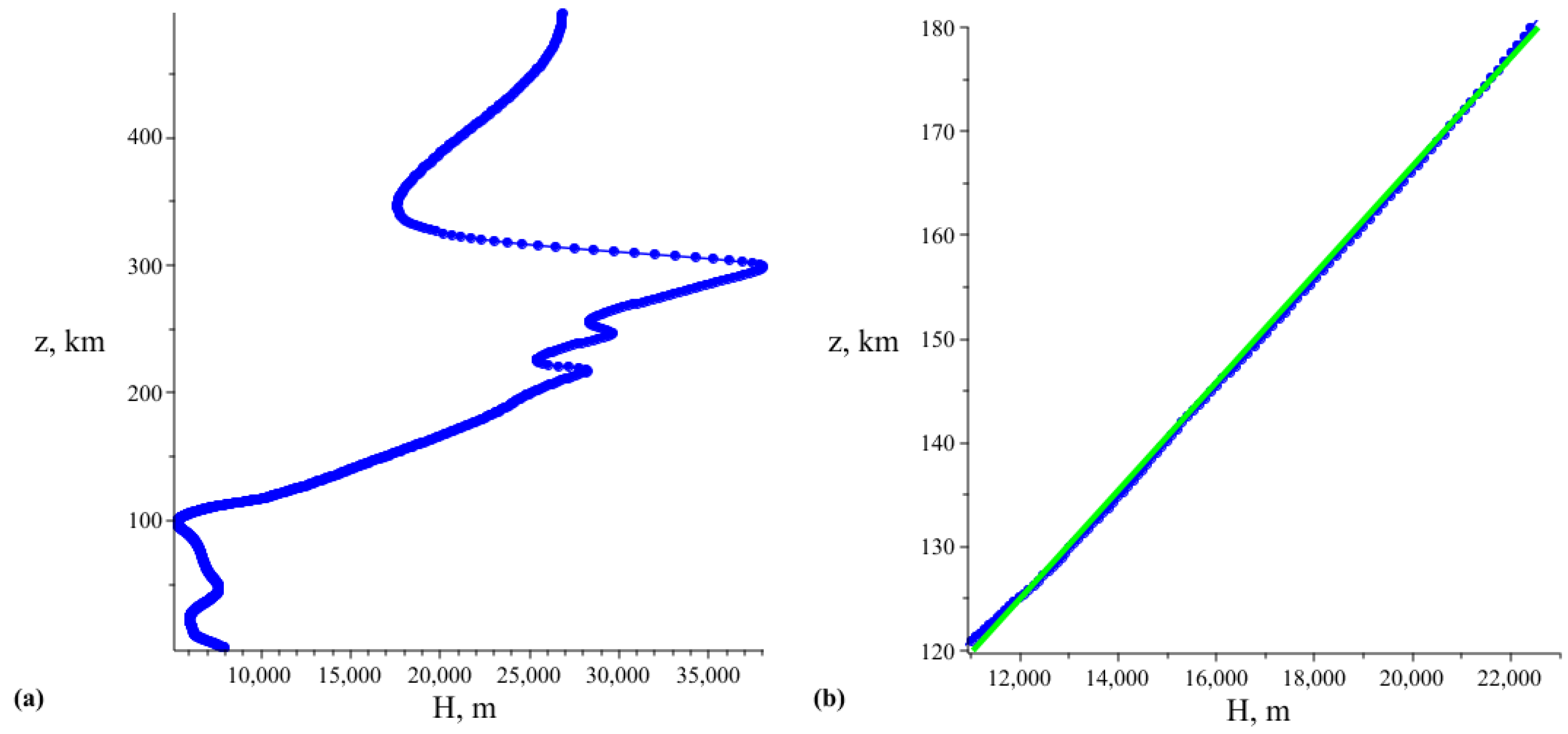
3.1. Standard Atmosphere H(z) Profile

In this section we prepare the atmosphere characteristics for numerical calculations, starting from the atmospheric scale height as follows

$$H\left(z_i\right)=H_i=\frac{R_{s}T\left(z_i\right)}{g},$$

(25)

where $z_i$ is the i-row element of the discrete data array for vertical coordinate, $H_i$ is the value of the atmosphere scale height at the height $z_i$, $T\left(z_i\right)$ is the value of the temperature at the reference height $z_i$, $R_s=R/M=287.1$ J/(kg·K) is the specific gas constant for dry air [24].

The height scale profile in Figure 2a corresponds to the table for background temperature $T\left(z_i\right)$, taken from [24].

Figure 2. (a) The atmosphere’s scale height $H\left(z_i\right)$ profile obtained according to the formula (25) [24]; (b) The atmosphere’s scale height $H\left(z_i\right)$ for $z_i$ within 120 km to 180 km range (in blue) and its linear approximation represented by formula (27) (in green).

The function (10) we approximate as follows

$${\nu }_i\left(z_i\right)=\gamma -1+\gamma \frac{dH\left(z\right)}{dz}{|}_{z=z_i}\approx \gamma -1+\gamma \frac{H_{i+1}-H_{i-1}}{z_{i+1}-z_{i-1}}.$$

(26)

The expression shows how we estimate the derivatives (excluding the first and last points, where the left and right derivatives approximations are used).

3.2. Linear Approximation of H(z)

According to the graph for the atmosphere’s scale height in Figure 2a, we will focus on the approximately linear part in the interval z $\in [120,180]$ km.

Note, that the difference between the dependence of $H\left(z\right)$ taken from the dataset and the linear approximations, given in Figure 2b within 120 km to 180 km range, is almost invisible at such scale. This gives an argument to use the linear approximation in further modelling. To provide the model test, we put $H\left(z\right)$ depending linearly on the coordinate z like:

$$H\left(z\right)=\alpha z-H$$

(27)

where the curves at the Figure 2b adjustment is provided by the choice of $H=12$,$000\mathrm{m}$, $\alpha =0.192$. The function $H\left(z\right)$ graph is shown in green in Figure 2b.

For the linear $H\left(z\right)$, the function (10) is:

$$\nu \left(z\right)=\gamma -1+\gamma \frac{dH\left(z\right)}{dz}=\gamma -1+\gamma \alpha .$$

(28)

4. Solution of a Disgnostic Equation for Linear Dependence of H(z) by Factorization Method

4.1. Operator Factorization

Let us choose the Equation (21), where

$$1-D_a{D}_0=1-{\gamma }^2\frac{{\left(H\left(z\right)\right)}^2}{\nu \left(z\right)}\frac{{\partial }^2}{\partial z^2}-2\alpha \gamma ·\gamma \frac{H\left(z\right)}{\nu \left(z\right)}\frac{\partial }{\partial z}+\frac{{\gamma }^2+2\alpha {\gamma }^2}{4\nu \left(z\right)},$$

(29)

for the entropy mode $(1-D_a{D}_0)P_0=f_0,$ or, on base of linear approximation of $H\left(z\right)$, it, by the factorization, may be rewritten as

$$\left(D^2+ED-A\right)P_0=\left(D-\varphi \right)\left(D-\psi \right)P_0=-\left(\gamma +\alpha \gamma -1\right)f_0=-\nu \left(z\right)f_0,$$

(30)

where, for the factorization convenience, the following expressions are introduced

$$D=\gamma H\left(z\right)\frac{\partial }{\partial z},E=\alpha \gamma ,A=\frac{{\gamma }^2+2\alpha {\gamma }^2}{4},$$

(31)

$$\varphi =E-\psi ,$$

(32)

$$\psi =\frac{1}{2}\sqrt{E^2+4A}-\frac{1}{2}E.$$

(33)

The operator of the second diagnostic Equation (23) for the acoustic mode is opposite to one of the first diagnostic equation, hence its solution differs only by the RHS (inhomogeneity).

4.2. On Boundary Conditions

4.2.1. General Remarks

A statement of the problem for the second order equations as (21) and (23) implies two boundary conditions either at the ends of the interval of consideration or both at one end of the heights range.

Generally, the inhomogeneous equation with the linear operator A

$$Au=f_0$$

(34)

is solved up to general solution of the homogeneous one:

$$u=A^{-1}{f}_0+u_h,$$

(35)

$$A{u}_h=0.$$

(36)

The function $u_h$ is fixed by a set of boundary conditions. In the case of the second order differential equation, we should choose two such conditions that determine the constants $C,C_1$.

In the problem of diagnostics, its formulation is more complicated. We have two ODE for the variables $P_0$ and $P_a$ of the same form of the operator, but with different RHS, The statement of the problem should also keep the condition

$$P_0+P_a=P,$$

(37)

within the whole range of the problem including the boundary.

4.2.2. Boundary Problem

The condition (37) being read literally, impose the condition

$$P_a\left(z_2\right)=P\left(z_2\right)-P_0\left(z_2\right).$$

(38)

It, together with

$$P_0\left(z_1\right)=0,P_0^{\prime }\left(z_1\right)=0,$$

(39)

and

$$P_a\left(z_1\right)=P\left(z_1\right)$$

(40)

closes the diagnostics problem formulation we investigate within this work.

The detailed solution to the first and second diagnostic equations is presented in the Appendix A.

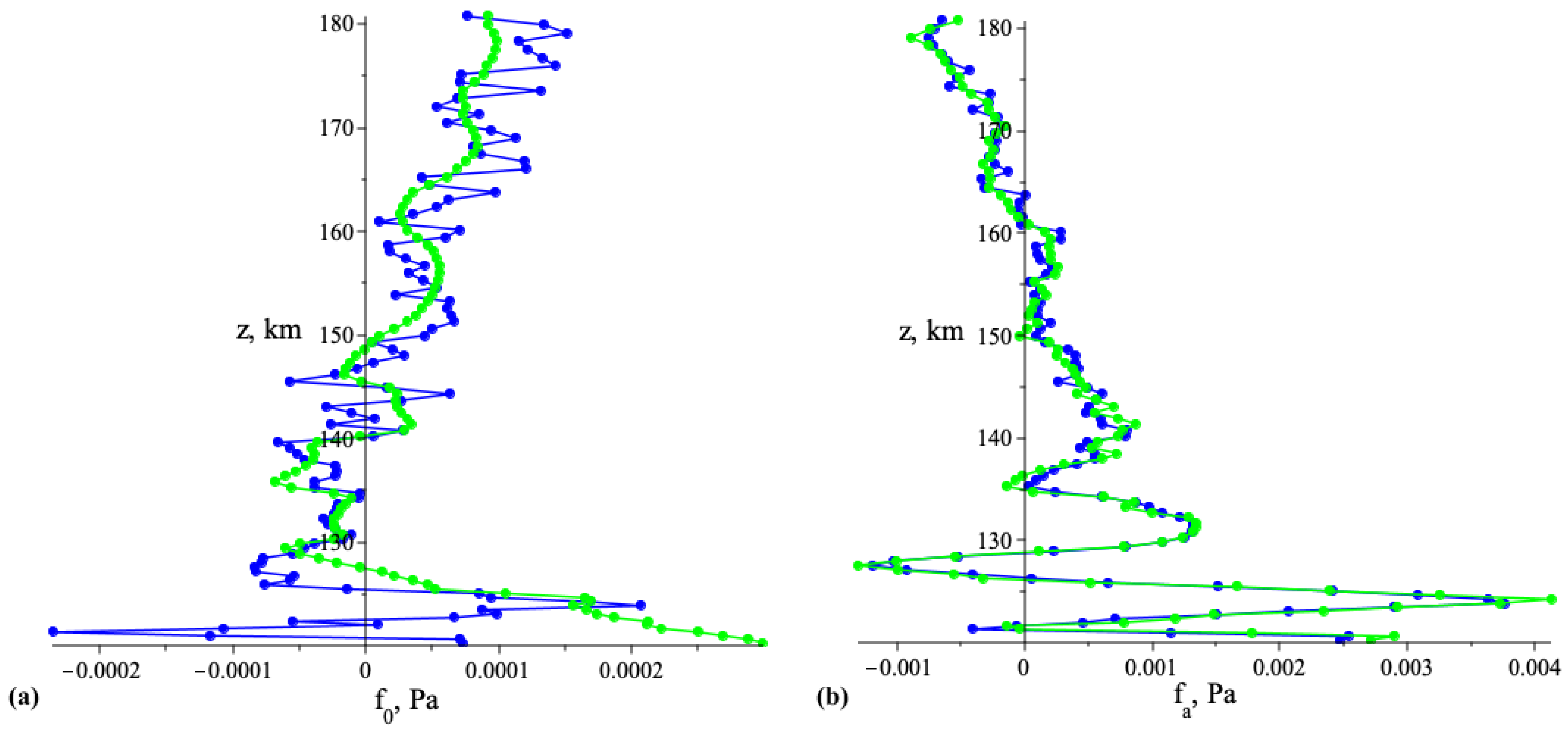
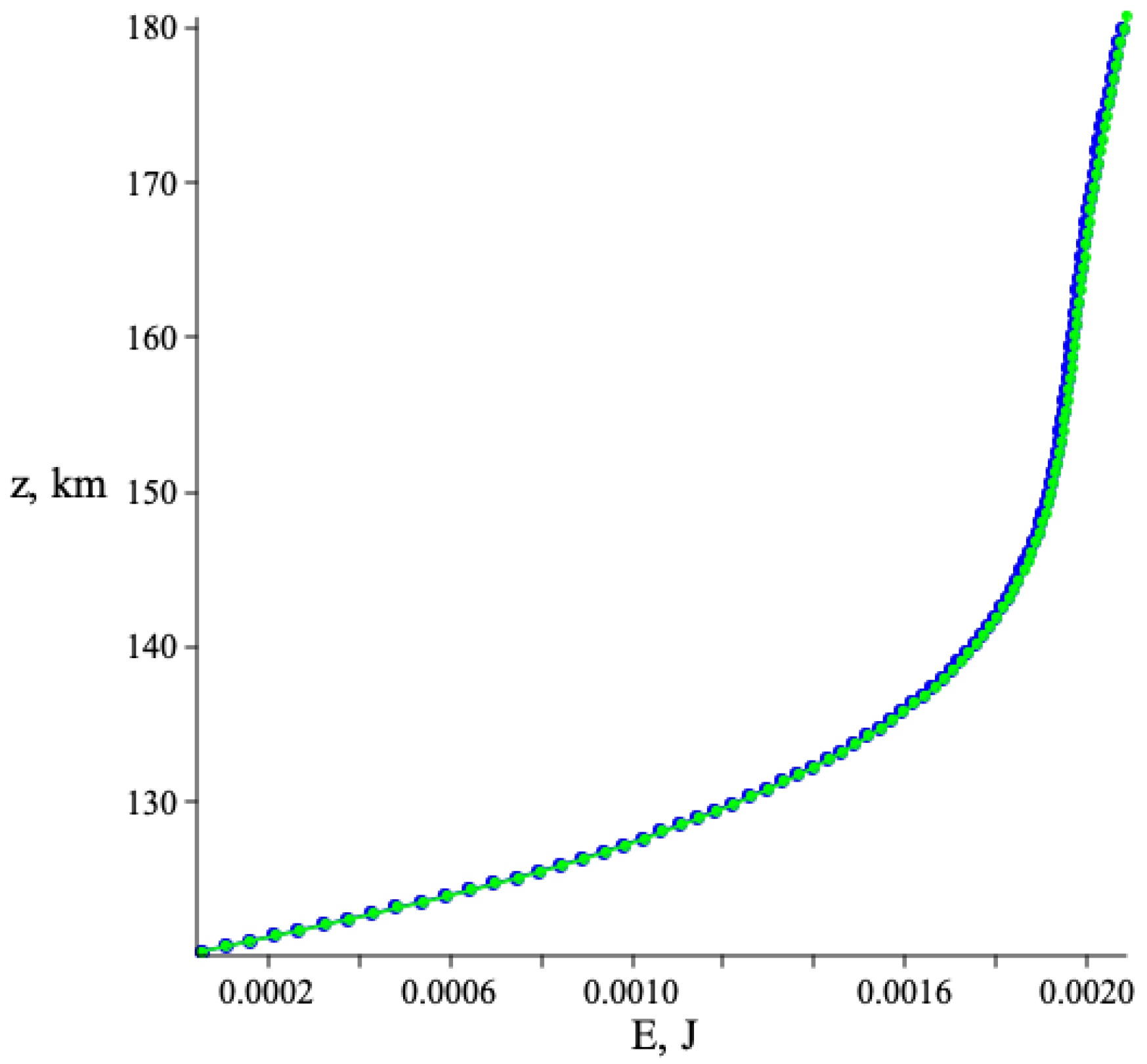
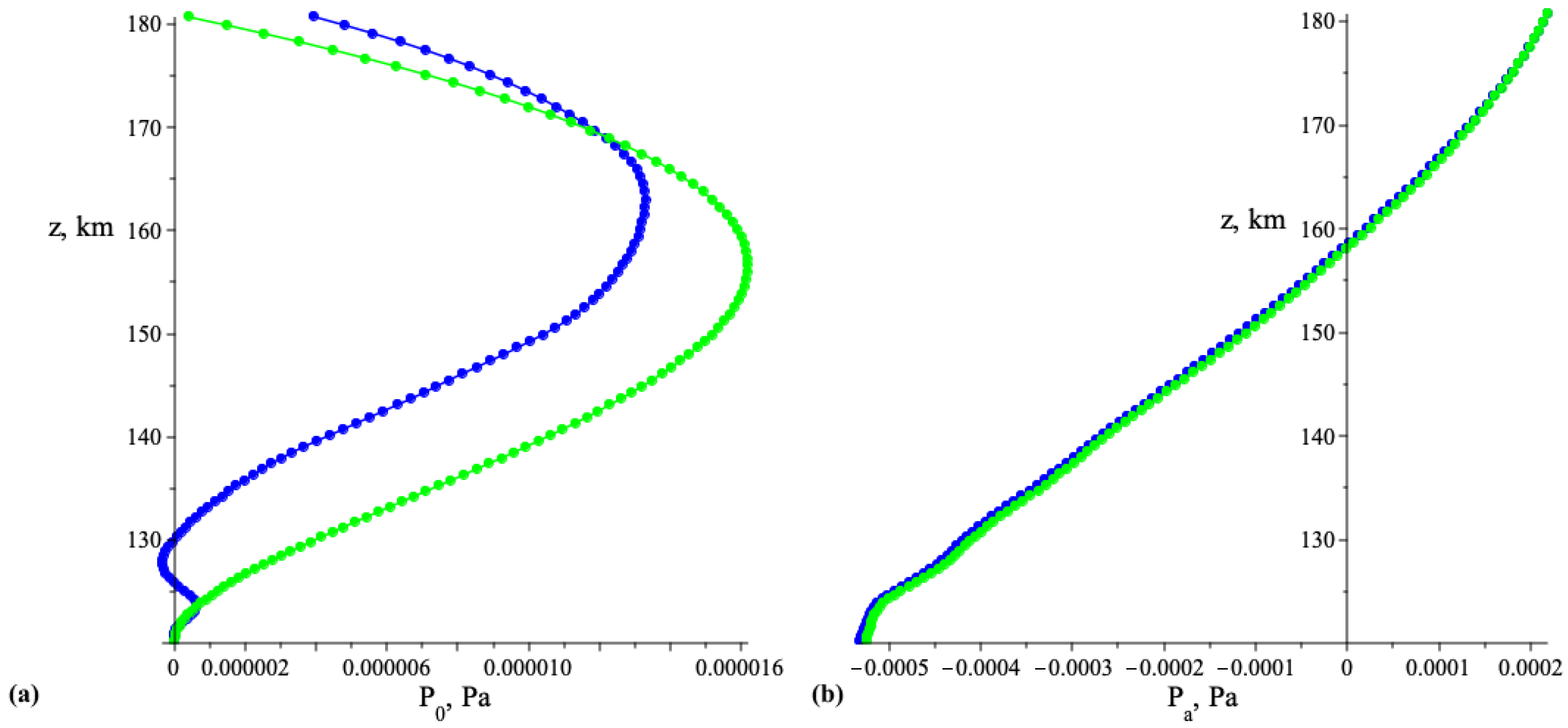
5. Applications to Data of a Numeric Experiment

5.1. Discrete Representation of Functions and Operators for the Standard Atmosphere H(z) Case

It follows from (21) that:

$$f_0\left(z_i\right)=P_i+D_{a,i}{\mathsf{\Phi }}_i,$$

(41)

where according to (15):

$$D_{a,i}=-\frac{\gamma -2}{2{\nu }_i\left(z_i\right)}-\gamma \frac{H_i}{{\nu }_i\left(z_i\right)}\frac{\partial }{\partial z}-\gamma {\left(\frac{H\left(z\right)}{{\nu }_i\left(z\right)}\right)}^{\prime }{|}_{z=z_i}.$$

(42)

In the same way the function (23)

$$f_a\left(z_i\right)=D_{a,i}{D}_{0,i}{P}_i+D_{a,i}{\mathsf{\Phi }}_i,$$

(43)

where according to (16):

$$D_{0,i}=\frac{\gamma -2}{2}-\gamma H_i\frac{\partial }{\partial z}.$$

(44)

The functions $P_i$ and ${\mathsf{\Phi }}_i$ are defined by means of dataset using formulas (4) and (5) which for the real $H\left(z_i\right)$ take the forms:

$$P_i=P\left(z_i\right)=p^{\prime }\left(z_i\right)·exp\left(\underset{0}{\overset{z_i}{\int }}\frac{d{z}^{\prime }}{2H\left(z^{\prime }\right)}\right)\approx p^{\prime }\left(z_i\right)·exp\left(\sum _{j=1}^i\frac{\Delta z_j}{2H\left(z_j\right)}\right),$$

(45)

$${\mathsf{\Phi }}_i=\mathsf{\Phi }\left(z_i\right)={\phi }^{\prime }\left(z_i\right)·exp\left(\underset{0}{\overset{z_i}{\int }}\frac{d{z}^{\prime }}{2H\left(z^{\prime }\right)}\right)\approx {\phi }^{\prime }\left(z_i\right)·exp\left(\sum _{j=1}^i\frac{\Delta z_j}{2H\left(z_j\right)}\right).$$

(46)

5.2. Representation of Functions and Operators for the Linear H(z) Case

For linear approximation of $H\left(z\right)$ of the form (27), the operators (15) and (16) have the forms:

$$D_a=-\left(\frac{\gamma -2}{2(\gamma -1+\gamma \alpha )}+\gamma \frac{\partial }{\partial z}\frac{\alpha z-H}{\gamma -1+\gamma \alpha }\right),$$

(47)

$$D_0=-\left(-\frac{\gamma -2}{2}+\gamma (\alpha z-H)\frac{\partial }{\partial z}\right).$$

(48)

For linear dependence of $H\left(z\right)$, the function $f_0\left(z\right)$ from (21) can be calculated as:

$$f_0\left(z\right)=P+D_a\mathsf{\Phi }=P-\frac{\gamma -2+2\alpha \gamma }{2(\gamma -1+\gamma \alpha )}\mathsf{\Phi }-\frac{\gamma (\alpha z-H)}{\gamma -1+\gamma \alpha }\frac{\partial \mathsf{\Phi }}{\partial z}$$

(49)

and function $f_a\left(z\right)$ from (23) takes the form:

$$f_a\left(z\right)=D_a{D}_{0}P+D_a\mathsf{\Phi }=\frac{1}{\gamma -1+\gamma \alpha }(-\frac{1}{4}(\gamma -2)(\gamma -2+2\alpha \gamma )P+$$

$$+2\alpha {\gamma }^2(\alpha z-H)\frac{\partial P}{\partial z}+{\gamma }^2{(\alpha z-H)}^2\frac{{\partial }^{2}P}{\partial z^2}-\frac{1}{2}(\gamma -2+2\alpha \gamma )\mathsf{\Phi }-\gamma (\alpha z-H)\frac{\partial \mathsf{\Phi }}{\partial z}),$$

(50)

where pressure and entropy perturbation functions (4) and (5) are:

$$P=p^{\prime }·exp\left(\underset{z_1}{\overset{z}{\int }}\frac{d{z}^{\prime }}{2H\left(z^{\prime }\right)}\right)=p^{\prime }·exp\left(\frac{1}{2\alpha }\left(ln(\alpha z-H)-ln(\alpha z_1-H)\right)\right),$$

(51)

$$\mathsf{\Phi }={\phi }^{\prime }·exp\left(\underset{z_1}{\overset{z}{\int }}\frac{d{z}^{\prime }}{2H\left(z^{\prime }\right)}\right)={\phi }^{\prime }·exp\left(\frac{1}{2\alpha }\left(ln(\alpha z-H)-ln(\alpha z_1-H)\right)\right).$$

(52)

Here, $z_1$ denotes the initial coordinate or in the case of a discrete dataset for the vertical coordinate. The above formulas yield:

$$P\left(z_i\right)=p^{\prime }·exp\left(\frac{1}{2\alpha }\left(ln\left(H\left(z_i\right)\right)-ln(\alpha z_1-H)\right)\right),$$

(53)

$$\mathsf{\Phi }\left(z_i\right)={\phi }^{\prime }·exp\left(\frac{1}{2\alpha }\left(ln\left(H\left(z_i\right)\right)-ln(\alpha z_1-H)\right)\right).$$

(54)

6. Comparison of the Models and Discussion of the Results

The oscillations of the RHSs of the diagnostic equations for $P_{0,a}$ (Figure 3), apart from a small variation of the function $H\left(z\right)$, appear due to the application of differentiation operation to the dataset components as in (42), which scale of coordinate differences and errors are noticeable.

Figure 3. Comparison of the functions $f_0\left(z\right)$ (a) and $f_a\left(z\right)$ (b) obtained using the formulas (41), (43) (49) and (50), respectively, for the cases of standard atmosphere $H\left(z\right)$ (25) (in blue) and linear height scale dependence $H\left(z\right)$ model (27) (in green).

Figure 4 shows the result of the diagnosis, namely the vertical structure of $P_{0,a}$ in the total pressure perturbation P. It looks much more smooth because its evaluation makes use of integration that acts as a “smoothing” operation, as opposite to differentiation. Such phenomena are well-known in the theory of inverse problems.

Figure 4. Comparison of the entropy mode $P_0\left(z\right)$ (a) and the acoustic one $P_a\left(z\right)$ (b) obtained using the formulas (A2) and (A8), respectively, for the cases of standard atmosphere $H\left(z\right)$ (25) (in blue) and linear height scale dependence $H\left(z\right)$ model (27) (in green).

The plots of Figure 4 represent one of the principle result of this work: they show that there is a discrepancy between the profile obtained by the direct dataset processing and handling by means of the apparatus based on the analytical approximation of the theory elements. The difference, however, is not so big, and the linear model allows to estimate the entropy mode profile confidently. The addition of independent results of calculations of $P_0$ and $P_a$ gives the curve closely matching with the graph of a function P represented by formula (4), which is consistent with the main idea of the expansion into modes $P=P_0+P_a$. The transition to energy distribution leads to the results for which the difference almost disappear, see Figure 5.

Figure 5. Energy calculated by the Equation (55) for the cases of standard atmosphere (in blue) and linear dependence (in green) of the height scale $H\left(z\right)$ for $z\in [120,180]$ km, see the relation (27).

Speaking about the modes extraction at the level of the pressure-entropy vector disturbances field we observe the difference of the results, visible at the plots of the Figure 4. The difference (by module about 5 percents) is due to the significant non-coincidence of the functional parameter $\nu \left(z\right)$. Namely, it is constant, in the case of the model (approximately equal to $0.79$), but varies, oscillating from $0.73$ to $0.92$, being calculated directly from standard atmosphere data $H\left(z\right)$, and being differentiated in (10) by means of the conventional derivative approximation. Estimation of $E\left(z\right)$, that is, the total energy of all modes at the coordinate range $[0,z]$, is given by the following expression

$$E\left(z\right)=\frac{1}{2}\underset{0}{\overset{z}{\int }}dz\left(\overline{\rho }{V}^2+\frac{p^{\prime 2}}{\gamma \overline{p}}+\frac{{\varphi }^{\prime 2}}{\gamma \nu \left(z\right)\overline{p}}\right),$$

(55)

and is represented by the profiles at Figure 5.

Note, that the energy profiles for the cases of the direct standard atmosphere and these based on explicit linear dependence are represented by the curves with scarcely visible difference (the difference is about the percent). Hence we propose to use the total energy values and the profiles (55) for the model mode weights estimation.

The authors believe that the analytical models are more desirable than numerical methods, which are usually time-consuming, require a high-performance computer, and special attention to underlying algorithms, their convergence, and stability investigation. On the other hand, reasonably simple analytical models, when complemented by a numerical approach, are much more efficient.

7. Conclusions

The main result of the presented work constitutes in the diagnostic equation, which solution gives the vertical profile of the acoustic and entropy modes contribution in the total wave perturbation. These results are applied to the realistic numerical modelling of the atmospheric perturbations by a source positioned near the Earth surface.

The next result of the study represents the diagnostic algorithm that uses the restricted heights interval, at which the $H\left(z\right)$ dependence is very close to linear. Its restriction guarantees the stability condition and the positively defined energy density. Usage of approximation on z allows proceeding with the diagnostic equation solution in explicit form. The resulting diagnostic predictions are compared with the results of numerical calculations at the whole available heights range under consideration. The extracted acoustical and entropy modes are extracted from the total perturbation field. The plots are compared with the model results.

One of the important ingredients of diagnostics is the possibility to estimate the relative weight of any mode contribution. It is also important to evaluate an error of this estimation, cumulative measurements errors and the theoretical and numerical discrepancies. Such possibility is directly based on the energy density definition with the positive functional parameter $\nu \left(z\right)$ at a height range under consideration. This has an impact on the norm definition in a functional space of the state vector.

References

- Kovasznay, L.S.G. Turbulence in Supersonic Flow. J. Aeronaut. Sci. 1953, 20, 657–674. [Google Scholar] [CrossRef]
- Chu, B.-T.; Kovásznay, L.S.G. Non-linear interactions in a viscous heat-conducting compressible gas. J. Fluid Mech. 1958, 3, 494. [Google Scholar] [CrossRef]
- Brekhovskikh, L.M.; Godin, A.O. Acoustics of Layered Media; Springer: Berlin, Germany, 1990. [Google Scholar]
- Pedloski, J. Geophysical Fluid Dynamics; Springer: New York, NY, USA, 1987. [Google Scholar]
- Gordin, A.V. Mathematical Problems of Hydrodynamical Weather Prediction. Analytical Aspects; Gydrometeoizdat: Leningrad, Russia, 1987. [Google Scholar]
- Leble, S.B. Nonlinear Waves in Waveguides with Stratification; Springer: Berlin, Germany, 1990. [Google Scholar]
- Wu, Y.; Llewellyn Smith, S.; Rottman, J.; Broutman, D.; Minster, J. The propagation of tsunami-generated acoustic–gravity waves in the atmosphere. J. Atmos. Sci. 2016, 73, 3025–3036. [Google Scholar] [CrossRef]
- Leble, S.; Perelomova, A. Dynamical Projectors Method in Hydro- and Electrodynamics; CRC Press, Taylor and Frensis Group: Boca Raton, FL, USA, 2018. [Google Scholar]
- Leble, S.; Perelomova, A. Problem of proper decomposition and initialization of acoustic and entropy modes in a gas affected by the mass force. Appl. Math. Model. 2013, 37, 629–635. [Google Scholar] [CrossRef]
- Belikovich, V.V.; Benediktov, E.A.; Tolmacheva, A.V.; Bakhmet’eva, N.V. Ionospheric Research by Means of Artificial Periodic Irregularities; Copernicus GmbH: Katlenburg-Lindau, Germany, 2002. [Google Scholar]
- Bakhmetieva, N.V.; Grigor’ev, G.I.; Tolmacheva, A.V. Artificial periodic irregularities, hydrodynamic instabilities, and dynamic processes in the mesosphere-lower thermosphere. Radiophys. Quantum Electron. 2011, 53, 623–637. [Google Scholar] [CrossRef]
- Leble, S.; Vereshchagin, S.; Bakhmetieva, N.; Grigoriev, G. On the Diagnosis of Unidirectional Acoustic Waves as Applied to the Measurement of Atmospheric Parameters by the API Method in the SURA Experiment. Atmosphere 2020, 11, 924. [Google Scholar] [CrossRef]
- Leble, S.; Vereshchagin, S.; Vereshchagina, I. Algorithm for the Diagnostics of Waves and Entropy Mode in the Exponentially Stratified Atmosphere. Russ. J. Phys. Chem. B 2020, 14, 371–376. [Google Scholar] [CrossRef]
- Leble, S.; Vereshchagina, I. Problem of disturbance identification by measurement in the vicinity of a point. Task Q. 2016, 20, 131–141. [Google Scholar]
- Butler, A.H.; Sjoberg, J.P.; Seidel, D.J.; Rosenlof, K.H. A sudden stratospheric warming compendium. Earth Syst. Sci. Data 2017, 9, 63–76. [Google Scholar] [CrossRef] [Green Version]
- Karpov, I.V.; Kshevetsky, S.P.; Borchevkina, O.P.; Radievsky, A.V.; Karpov, A.I. Disturbances of the upper atmosphere and ionosphere caused by acoustic-gravity wave sources in the lower atmosphere. Russ. J. Phys. Chem. B 2016, 10, 127–132. [Google Scholar] [CrossRef]
- Kshevetskii, S.P.; Kurdyaeva, Y.A.; Gavrilov, N.M.; Karpov, I.V. Simulation of vertical propagation of acoustic-gravity waves in the atmosphere based on variations of atmospheric pressure and research of heating of the upper atmosphere by dissipated waves. In Proceedings of the V International Conference Atmosphere, Ionosphere, Safety; Publishing house of the Baltic Federal University. I. Kant: Kaliningrad, Russia, 2016; pp. 468–473. [Google Scholar]
- Kshevetskii, S.P.; Kurdyaeva, Y.A. The Numerical Study of Impact Of Acoustic-Gravity Waves from the Pressure Source on The Earth’s Surface on the Thermosphere Temperature. Tr. Kol‘skogo Nauchnogo Czentra RAS 2016, 4, 161–166. [Google Scholar]
- Kurdyaeva, Y.A.; Kshevetski, S.P.; Gavrilov, N.; Kulichkov, S.N. Correct boundary conditions for the high-resolution model of nonlinear acoustic-gravity waves forced by atmospheric pressure variations. Pure Appl. Geophys. 2018, 175, 3639–3652. [Google Scholar] [CrossRef]
- Brezhnev, Y.; Kshevetsky, S.; Leble, S. Linear initialization of hydrodynamical fields. Atmos. Ocean. Phys. 1994, 30, 84–88. [Google Scholar]
- Sun, L.; Robinson, W.A.; Chen, G. The predictability of stratospheric warming events: More from the troposphere or the stratosphere? J. Atmos. Sci. 2012, 69, 768–783. [Google Scholar] [CrossRef] [Green Version]
- Perelomova, A. Weakly nonlinear dynamics of short acoustic waves in exponentially stratified gas. Arch. Acoust. 2009, 34, 127–143. [Google Scholar]
- Zettergren, M.D.; Snively, J.B. Ionospheric response to infrasonic- acoustic waves generated by natural hazard events. J. Geophys. Res. Space Phys. 2015, 120, 8002–8024. [Google Scholar] [CrossRef] [Green Version]
- U.S. Government Printing Office. U.S. Standard Atmosphere; U.S. Government Printing Office: Washington, DC, USA, 1976. [Google Scholar]
- Leble, S.; Perelomova, A. Decomposition of acoustic and entropy modes in a non-isothermal gas affected by a mass force. Arch. Acoust. 2018, 43, 497–503. [Google Scholar]
- Perelomova, A. Nonlinear dynamics of directed acoustic waves in stratified and homogeneous liquids and gases with arbitrary equation of state. Arch. Acoust. 2000, 25, 451–463. [Google Scholar]
- Perelomova, A. Nonlinear dynamics of vertically propagating acoustic waves in a stratified atmosphere. Acta Acust. 1998, 84, 1002–1006. [Google Scholar]
- Leble, S.; Smirnova, E. Tsunami-Launched Acoustic Wave in the Layered Atmosphere: Explicit Formulas Including Electron Density Disturbances. Atmosphere 2019, 10, 629. [Google Scholar] [CrossRef] [Green Version]
- AtmoSym: A Multi-Scale Atmosphere Model from the Earth’s Surface up to 500 km. 2016. Available online: http://atmos.kantiana.ru (accessed on 10 April 2017).
Publisher’s Note: MDPI stays neutral with regard to jurisdictional claims in published maps and institutional affiliations. |
© 2021 by the authors. Licensee MDPI, Basel, Switzerland. This article is an open access article distributed under the terms and conditions of the Creative Commons Attribution (CC BY) license (https://creativecommons.org/licenses/by/4.0/).