Latitudinal Dependence of the Ionospheric Slab Thickness for Estimation of Ionospheric Response to Geomagnetic Storms

Abstract

The changes in the ionosphere during geomagnetic disturbances is one of the prominent Space Weather effects on the near-Earth environment. The character of these changes can differ significantly at different regions on the Earth. We studied ionospheric response to five geomagnetic storms of March 2012, using data of Total Electron Content (TEC) and F2-layer critical frequency (foF2) along the meridian of 70° W in the Northern Hemisphere. There are few ionosondes along this longitudinal sector: in Thule, Sondrestrom, Millstone Hill and Puerto Rico. The lacking foF2 values between the ionosondes were determined by using the experimental latitudinal dependences of the equivalent ionospheric slab thickness and TEC values. During geomagnetic storms, the following features were characteristic: (a) two-hours (or longer in one case) delay of the ionospheric response to disturbances, (b) the more prominent mid-latitude trough and (c) the sharper border of the EIA northern crest. During four storms of 7–17 March, the general tendency was the transition from negative disturbances at high latitudes to intense positive disturbances at low latitudes. During the fifth storm, the negative ionospheric disturbance controlled by O/N₂ change was masked by the overall prolonged electron density increase during 21–31 March. The multiple correlation analysis revealed the latitudinal dependence of dominant Space Weather parameters’ impacts on foF2.

1. Introduction

Space Weather conditions influence on the ionosphere, whose state defines the reliability of operation of different technological systems [1,2]. Ionospheric response to geomagnetic disturbances depends on the latitude and can be estimated with two main ionospheric parameters: critical frequency of the F2-layer (foF2) and vertical Total Electron Content (TEC). Both foF2 and TEC characterize the state of the ionosphere and have common features, but are not interchangeable, as it was shown, for example, in References [3,4,5]. For a comprehensive diagnostics of the ionosphere, it is preferable to have information about the changes of both parameters. The networks of ionosondes that perform direct foF2 measurements have less spatial coverage if compared to the networks of Global Navigation Satellite System (GNSS) receivers that provide raw data for TEC calculation. Global Ionospheric Maps (GIM) based on data from International GNSS Service receivers provide spatial TEC resolution of 5° in longitude and 2.5° in latitude worldwide [6]. When foF2 data are missed, they can be derived from TEC data indirectly (e.g., Reference [7]). It can be also done by using the equivalent slab thickness (τ) which is defined as a relation of TEC to the maximum electron concentration in the F2-layer (NmF2) [8]. Variations of τ have been discussed by many authors (see, for example, References [9,10,11,12,13,14]). The issue of foF2 reconstruction based on τ was discussed, for example, in References [15,16,17,18]. In the present work it is suggested to use the experimental median value of the ionospheric slab thickness τ(med) for this purpose. The idea is, first, to determine the experimental value of τ when the experimental values of both foF2 and TEC are available. This experimental τ can serve as a “reference” value. Further, it can be used to reconstruct foF2 missed values from the measured TEC values for the periods of interest. We used monthly median τ(med) as a reference value. It was calculated every two hours for each hour of the day separately. Equations (1)–(4) describe the foF2 reconstruction procedure.

foF2(rec) = 897 (NmF2(rec))^0.5,

(1)

NmF2(rec) = TEC(obs)/τ(med),

(2)

τ(obs) = TEC(obs)/NmF2(obs),

(3)

τ(med) = med(τ(obs))

(4)

There are different attempts to estimate Space Weather impacts on the ionospheric variations during storms (for examples, see References [19,20,21,22]). The ionospheric response to disturbances depends on the longitude and can differ significantly in different longitudinal sectors. The aim of this work was to study TEC and foF2 responses to geomagnetic disturbances during March 2012 along the of 290° E (70° W) meridian in Northern Hemisphere using the calculated latitudinal τ(med) dependence in this region. The mentioned disturbed period was suggested by SCOSTEP [23,24] as a subject for the comprehensive study. Our tasks were (1) to construct the latitudinal τ(med) dependence; (2) reconstruct the required foF2 values during disturbances through the obtained τ(med) and TEC(obs); (3) analyze TEC(obs) and foF2(rec) responses to five distinct geomagnetic storms in the considered longitudinal sector; and (4) make estimations of how the ionospheric parameters depended on Space Weather parameters (solar wind, interplanetary magnetic field and geomagnetic field) during the considered disturbances.

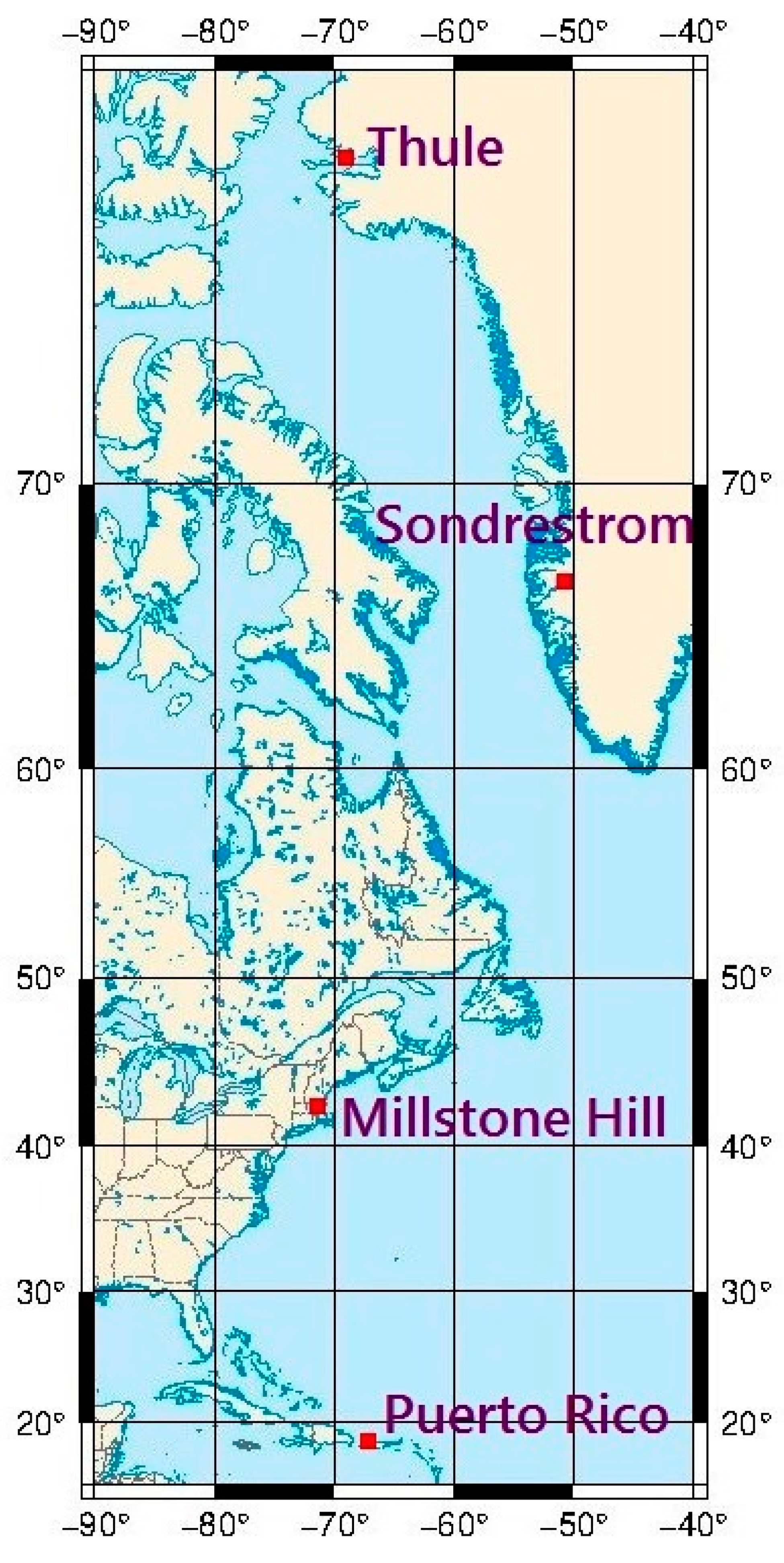
2. Experiments

We used critical frequency observational data foF2(obs) measured at four ionosondes installed along the mentioned meridian within the latitude range of (15°–80°) N. These four ionosondes belong to Digisonde Network [25] and have the following coordinates: Thule (77.5° N, 69.2° W), Sondrestrom (67° N, 50.9° W), Millstone Hill (42.6° N, 71.5° W), Puerto Rico (18.5° N, 67.2° W). Figure 1 illustrates the map of their locations. To obtain TEC(obs) values in the region, we used GIM data by Jet Propulsion Laboratory (JPL), California Institute of Technology, Pasadena, CA, USA [26].

The period of 7–17 March 2012 includes four magnetic storms of different intensity, which were triggered by different solar wind structures. The fifth storm of the month occurred on 27–29 March 2012.

Table 1. Parameters of geomagnetic storms during March 2012. MP, main phase; RP, recovery phase.

Storm №	MP Beginning	RP Beginning	Minimum Dst Value	Maximum Kp Value
1	7 March ~04 UT	7 March ~09 UT	−88 nT	6
2	9 March ~01 UT	9 March ~08 UT	−145 nT	8
3	12 March ~10 UT	12 March ~16 UT	−64 nT	6
4	15 March ~14 UT	15 March ~20 UT	−88 nT	6
5	27 March ~10 UT	28 March ~04 UT	−68 nT	5

provides information about the moments of storms’ main (MP) and recovery (RP) phase beginnings, Dst-index minimum and Kp-index maximum values. The events are numbered in order of their occurrence (first column). UT means Universal Time and LT means Local Time throughout the text. Figure 2 shows Space Weather parameters variations during the period of interest: solar radio flux at the wavelength of 10.7 cm (F10.7-index) that characterizes solar activity; Interplanetary Magnetic Field (IMF) magnitude and its Bz-component that characterize solar wind interaction with Earth’s magnetosphere; solar wind proton temperature; solar wind speed (V); proton density (Np) in the solar wind plasma and indices of geomagnetic activity Dst, AE and Kp, describing different processes in geomagnetic field variation [27,28,29,30,31,32]. Numbers 1–5 in Figure 2 correspond to the numbers of storm events in Table 1.

The review of geomagnetic storms of March 2012 was given in Reference [23] and references therein. It is important to emphasize that, in regard to geomagnetic field, the period of 7–17 March was non-quiet, which is clearly observed in variations of Dst and Kp indices (Figure 2) whose values during this period were systematically far from their quiet levels. Such a perturbed state was due to a highly structured interplanetary medium provoked by, at least, two simultaneous conditions. First, it was largely due to the presence of multiple coronal holes detected at Sun. Furthermore, the occurrence of several fast Coronal Mass Ejections (CMEs) played its role as their driven-shock waves changed the state of the interplanetary medium significantly. Therefore, strictly speaking, it is difficult to identify the exact beginning and end of each geomagnetic storm within this period, especially when its MP was not sufficiently intense or clear. We briefly mention the main triggers for each of five storms of March 2012 below. To identify them, the following CME catalogs were used: Richardson and Cane ICME List [33], CfA Interplanetary Shock Database, LASCO CME [34,35], CACTus [36] and SEEDS [37]; and the images by CHIMERA algorithm [38] for detection of coronal holes. In addition, the descriptions of interplanetary structure features in References [39,40,41] and references therein were helpful.

Storm №1 probably was triggered by the transit of a streams interacting region with southward Bz component of IMF. This interacting region was consistent with (caused by) the equatorial coronal hole observed in the Sun–Earth direction three days before the magnetic storm.

Storm №2 began with the sudden commencement caused by the shockwave arrival on 8 March. Some hours after the shock’s transit (early hours of 9 March), a region of southern Bz magnetic field appeared and lasted till the midday of 9 March, which marked the beginning of the RP of the storm. This magnetic region formed part of the magnetic structure (cloud) of the Interplanetary CME (ICME) (2012/03/07 0024-LASCO Catalog) associated with the shock wave mentioned above.

The abrupt increase of Dst at ~5 UT on 12 March marked the beginning of storm №3 and was probably caused by the shock wave arrival at Earth. Then, the magnetosheath behind the shock had the significant southern Bz-component with short duration, which resulted in the MP of the magnetic storm lasting several hours. Its RP began with the ICME arrival at the end of the day, as its magnetic structure was not sufficient to prolong the storm. It is important to highlight that the period of storm №3 is consistent with the possible transits of two interacting ICMEs: one detected at 2012/03/09-0426 and another at 2012/03/10-1800 (see LASCO Catalog). Therefore, the structure associated with storm №3 could be triggered by a complex event of two interacting ICMEs.

Storm №4 was triggered by the transit of the region with the southern Bz component of IMF, which was a part of the magnetic structure (cloud) of ICME whose transit in the near-Earth space lasted some hours. This is why the storm’s MP was short.

Finally, storm №5 was provoked by the southern Bz-component associated with the transit of a streams interacting region probably caused by the coronal hole observed on 14 March, at the solar equator. The southern Bz-component was oscillating, causing a variable electric field which in turn caused a slow and partially weak MP for this storm.

3. Results

In this section we assess the ionospheric behavior along the chosen longitudinal sector during the considered disturbances. First, τ was estimated according to Equations (1)–(4), for a further reconstruction of foF2 values. Then, TEC and foF2 variations were analyzed at different latitudes of the sector.

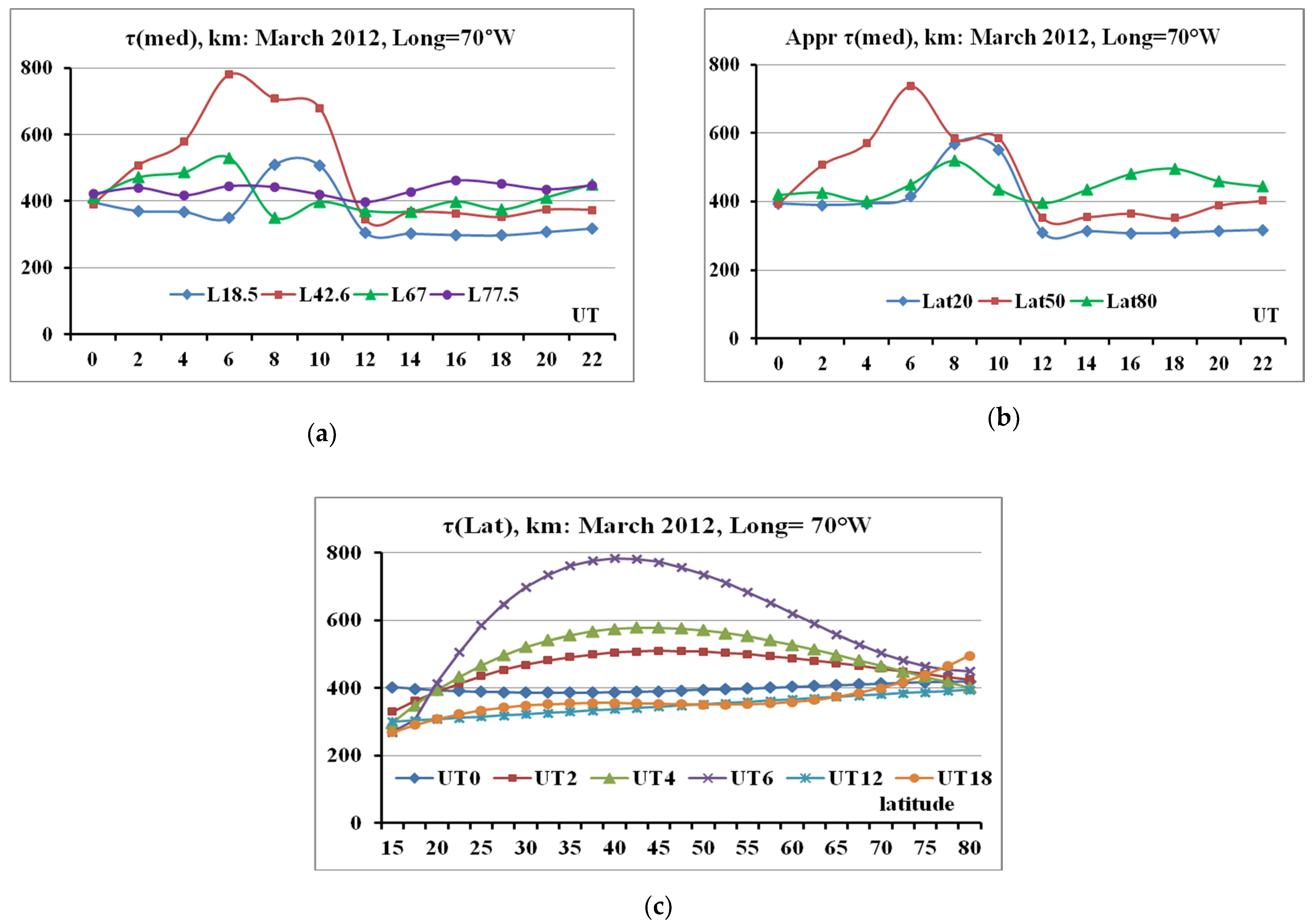
3.1. τ(med) Estimation for Different Latitudes

The ionosonde stations from Figure 1 are located at different latitudes. Therefore, τ(med) values calculated for these stations can be used to construct the latitudinal dependence of τ(med) for each hour. The parameter τ has its own independent meaning, as it provides the substantial information on the shape of the electron density profile, the neutral and ionospheric temperatures/gradients, the ionospheric composition and dynamics [42]. However, in the instant case, it has an ancillary character as a coefficient of proportionality between TEC and NmF2. Figure 3a shows the experimental τ(med) obtained at four ionosonde stations. It is seen that the mid-latitude ionosphere expands in the first half of the day by UT. During other hours, the range of τ variations is not large and has a tendency of increase with latitude. Diurnal variation of τ is obtained within the range of all latitudes with 2.5° step by constructing the polynomial of τ by four points. In this case, the polynomial of third degree provided the confidence factor close to 1 for all UT hours, except 12 UT (~7 LT). For the last case, the linear approximation with the confidence factor of 0.98 was sufficient. The examples of the diurnal variation calculated by polynomial are given in Figure 3b for three distinct latitudes at which the ionosonde measurements were not performed.

The latitudinal distribution of τ for the particular hours (UT) of the day in the considered longitudinal sector is presented in Figure 3c. An interesting feature was revealed for τ at 0 UT (~19 LT). It almost did not change with latitude having the value of about 400 km along the whole meridian. The τ for 12 and 18 UT (01 and 13 LT) did not change much between 30° N and 60° N. The large variations at other hours were due to the τ(med) behavior at the Millstone Hill station (Figure 3a).

To sum up, the latitudinal dependence of τ(med) was obtained with use of polynomial approximation and can be used to reconstruct foF2 latitudinal dependences from TEC data, as shown in Section 3.3.

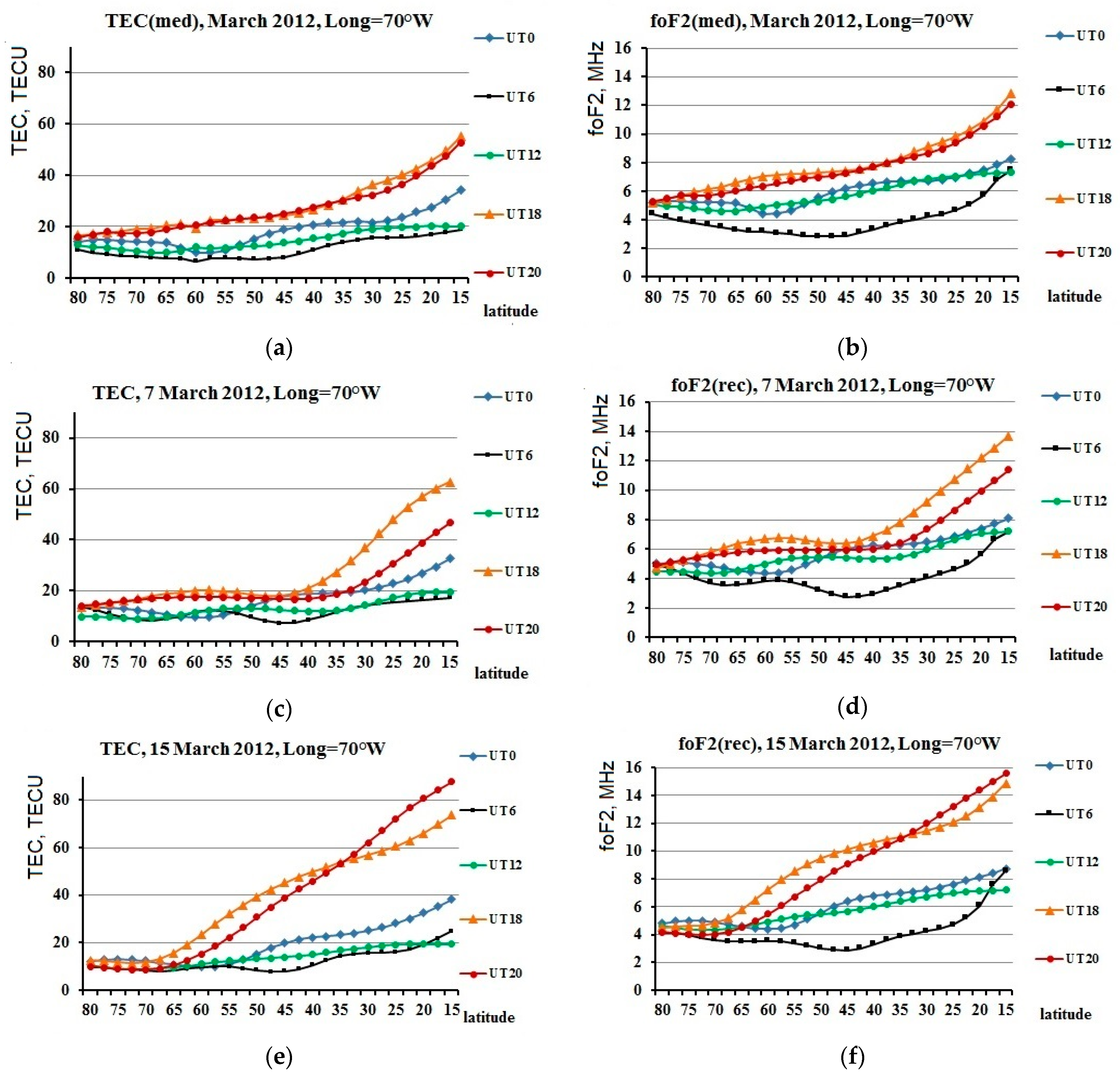
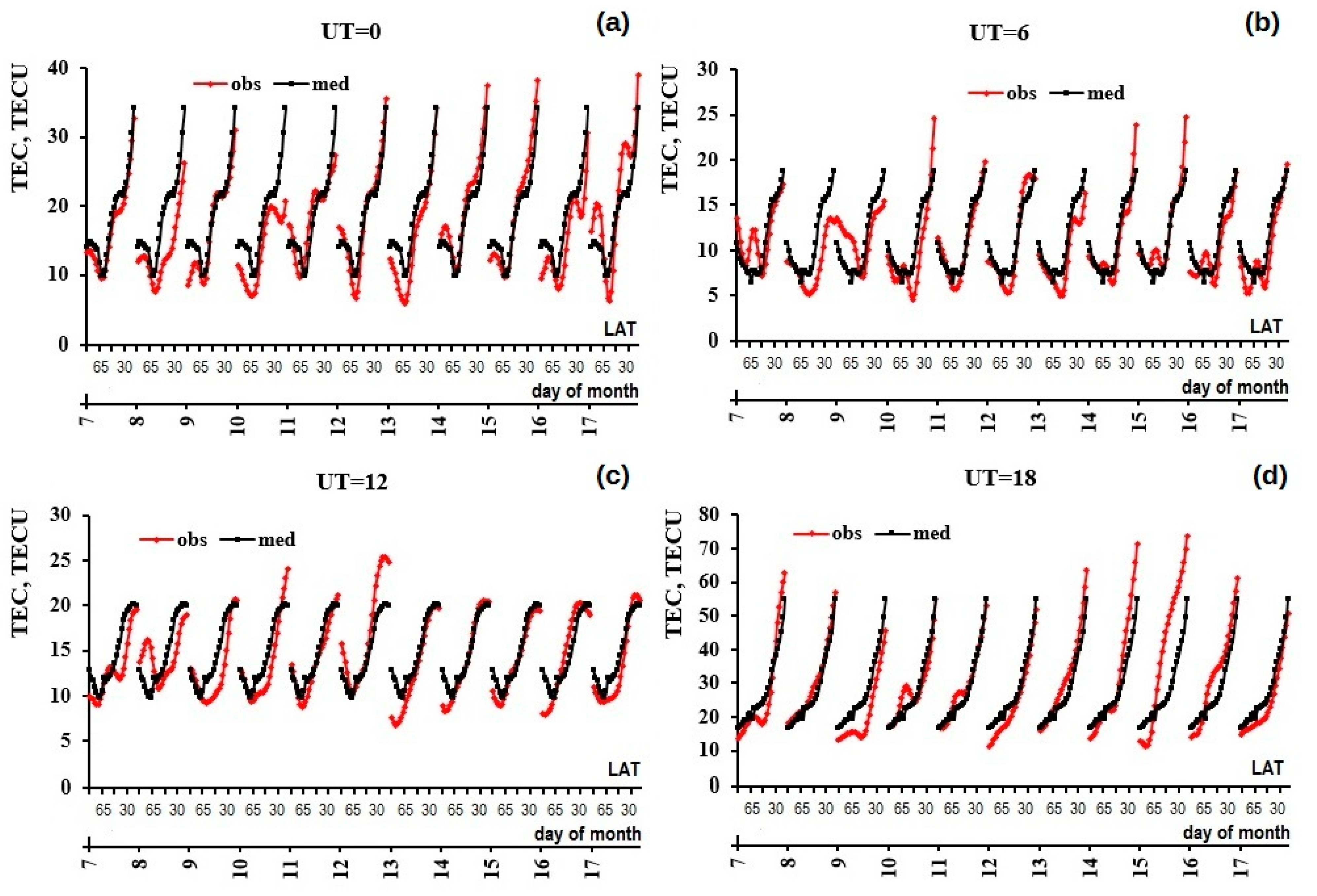
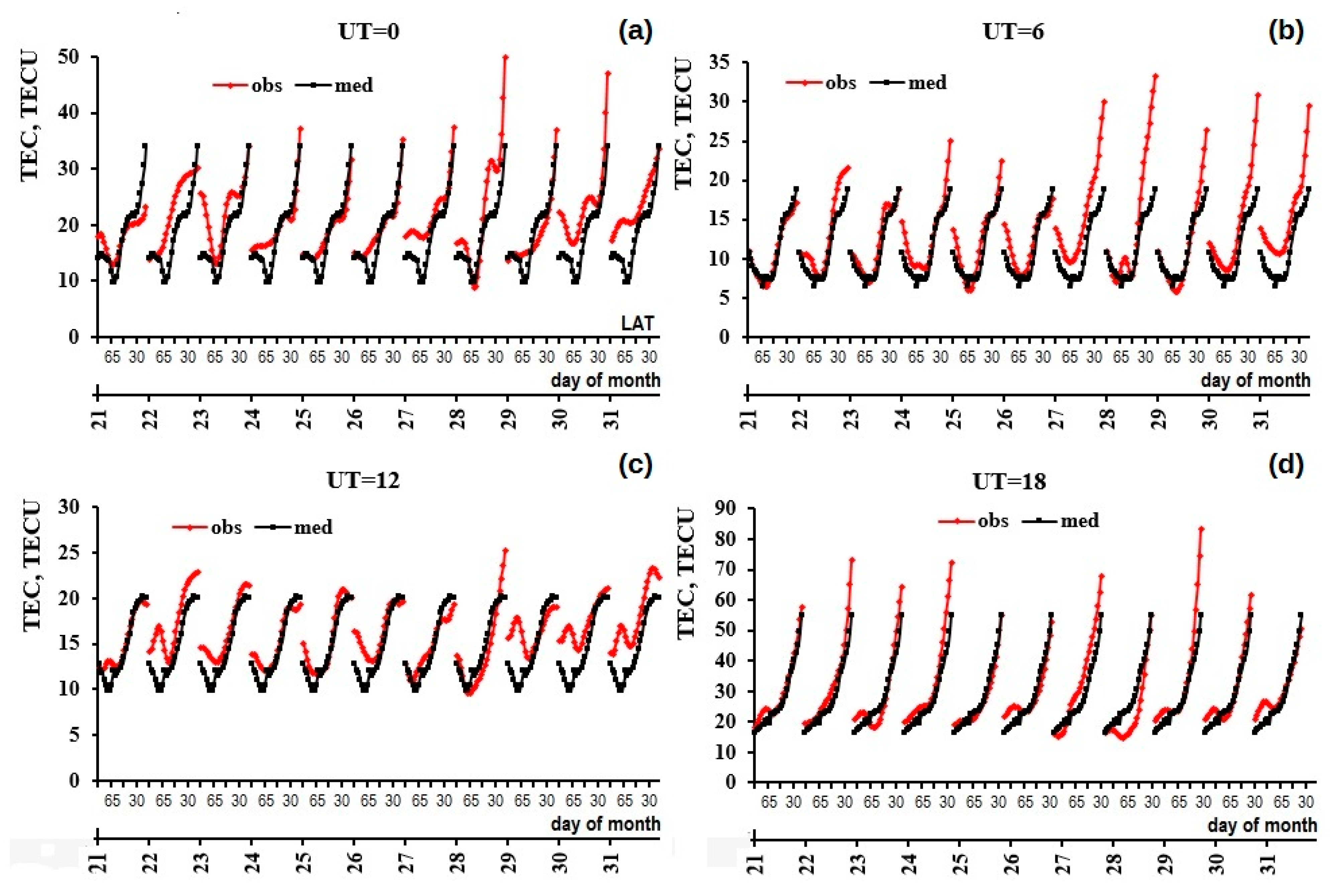
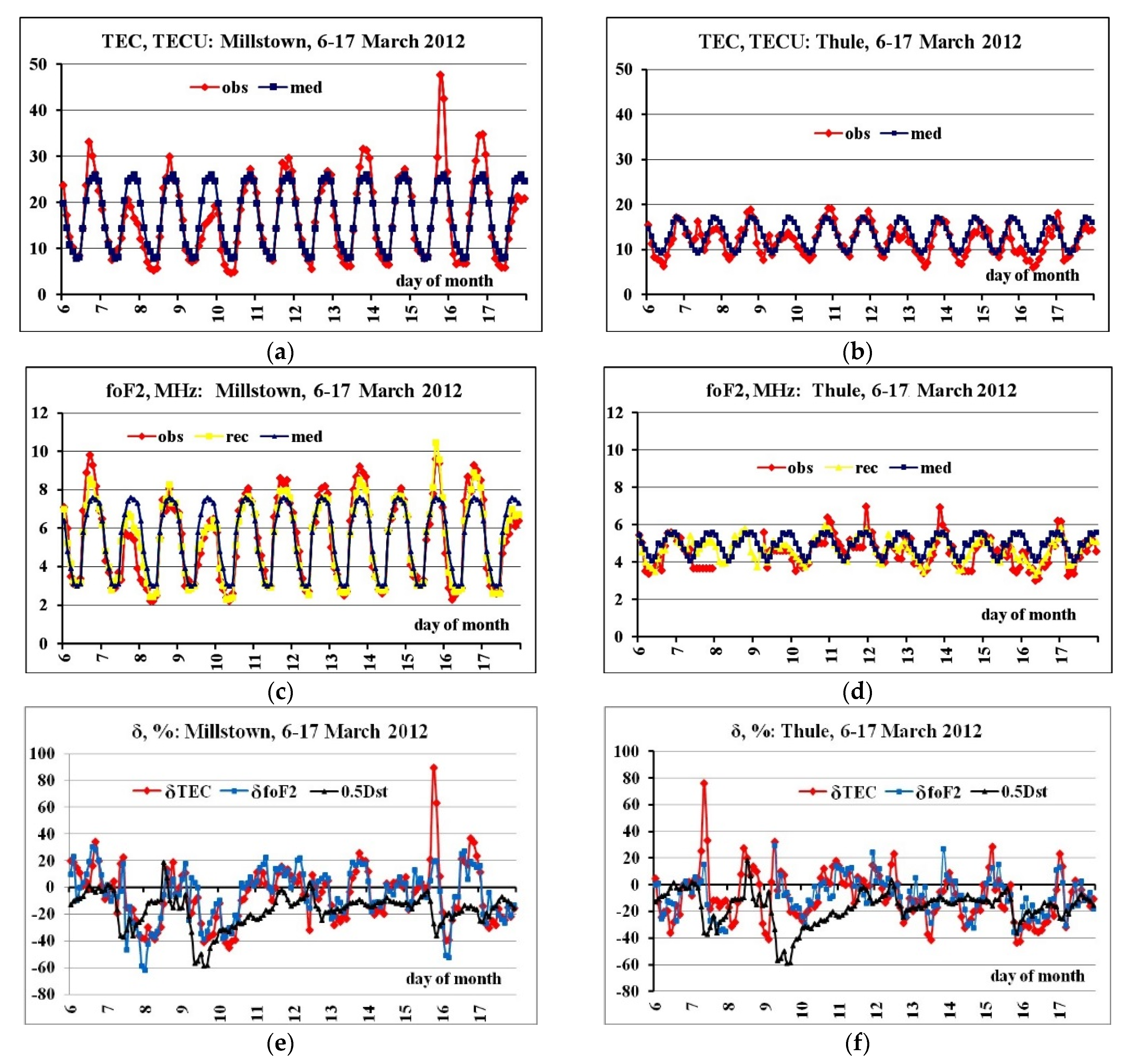
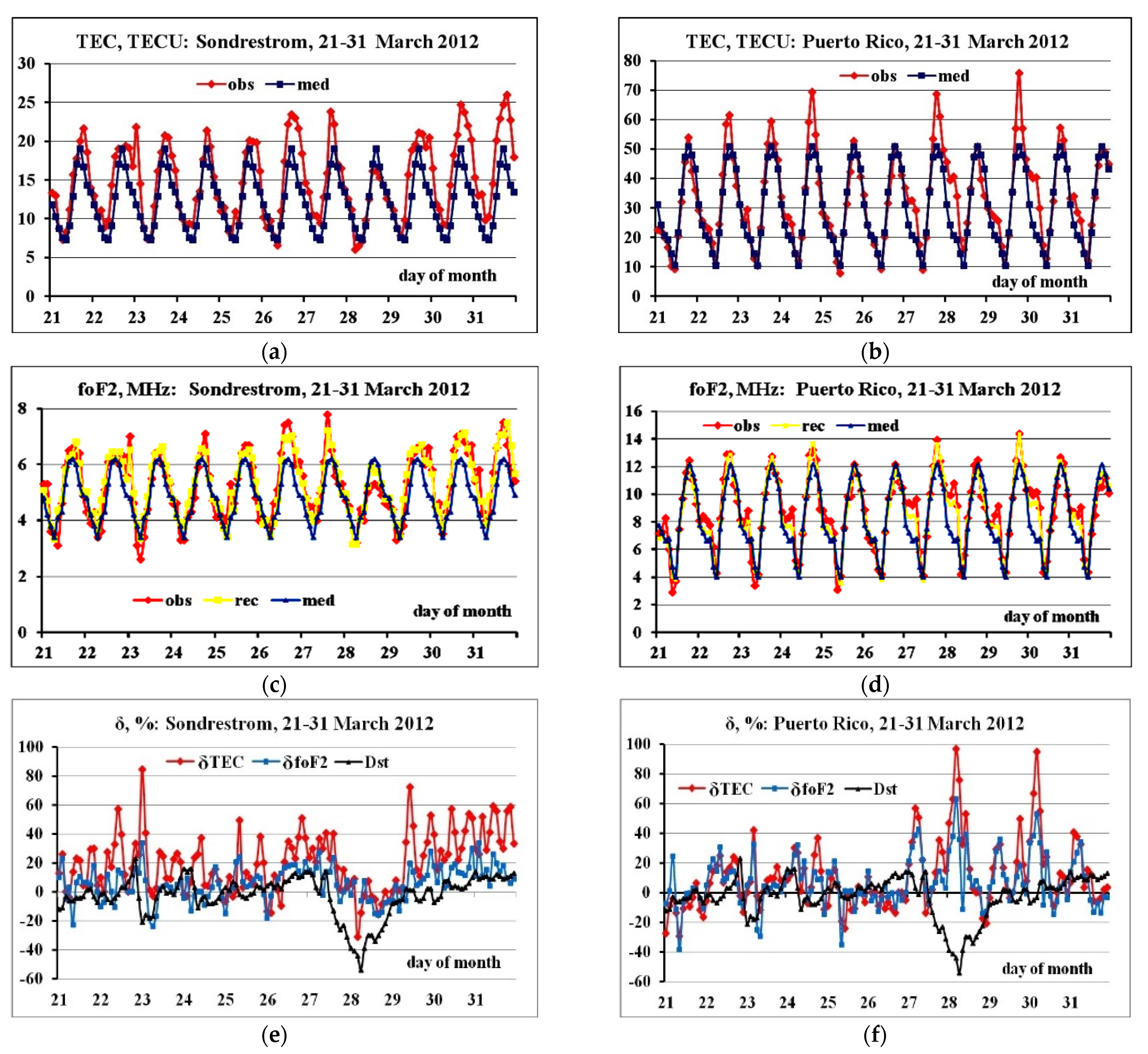
3.2. TEC Variations

Figure 4 (left panels) shows the monthly median TEC values for comparison (Figure 4a) and the examples of TEC behavior at different latitudes during geomagnetic storms (Figure 4c,e). Median values characterize TEC behavior under quiet conditions. These values are also used for estimation of deviations of instantaneous TEC (δTEC) which characterize the disturbance effect. Each curve stands for a particular UT hour: UT0 means local evening at ~19 LT; UT6 means local night at ~1 LT; UT12 local morning at ~7 LT and UT18-UT20 local near-midday hours ~(13–15) LT. Even at first glance, the picture of TEC during disturbances differed from the picture of median TEC variations. Comparison of plots in Figure 4 shows that the midday positive disturbances on 7 March and 15 March were more prominent in the low-latitude region. They were most intense on 15 March and covered the significantly large area up to the high latitudes. Right panels of the figure are discussed in Section 3.3.2.

Figure 5 shows the overall picture of latitudinal TEC variation (with a 2.5° latitude step) during 7–12 March in the considered longitude sector for evening, night, morning and day hours (0, 6, 12 and 18 UT). TEC values between the latitudes 80° N and 15° N (from left to right) for each day are shown in the plots. For the economy of space, only latitudes 65° and 30° are indicated in the X-axis. Each plot (panels a–d) is constructed for a particular UT hour characterizing evening, night, morning and daytime conditions. The significant influence of the magnetic storms on TEC and foF2 can be noted.

Figure 6 shows latitudinal dependences at the end of March 2012. It is seen that during the whole period of 21–31 March the ionosphere was not quiet. The curves of TEC(obs) differ significantly from their medians. TEC values under quiet geomagnetic conditions were mostly increased. During the storm itself (27–28 March) the difference between the median and observed TEC values was most pronounced at low latitudes.

The overall impression from Figure 5 and Figure 6 is that, during the series of geomagnetic disturbances of March 2012, the manifestation of the main ionospheric trough (MIT) and the electron density increase in the northern crest of Equatorial Ionization Anomaly (EIA) were much intense and, in general, the ionospheric structures were more pronounced. During the disturbed days, MIT moved to the lower latitudes and, in general, the electron concentration at high and mid latitudes was higher at evening, night and morning hours. This is due to the enhanced auroral ionization which is reflected in the AE-index bursts and confirmed by the MIT features (e.g., Reference [43]).

3.3. foF2 Variations

3.3.1. foF2 Reconstruction Validation

The foF2 values (foF2(rec)) were reconstructed during the considered multiple storm period according to Equations (1)–(4). First, we estimate how good is the accord between foF2(rec) and the observed values foF2(obs) measured by ionosondes. The time series of the observed TEC and reconstructed foF2, their corresponding monthly medians and deviations from these medians (δTEC and δfoF2) were plotted for all four ionosonde locations. The examples for Millstone Hill and Thule are illustrated in Figure 7.

The use of ionospheric parameters median values is the simplest approach to estimate/reveal (and even predict) the ionospheric systematic variations (diurnal, monthly, semi-annual, annual, etc.). Obviously, foF2(med) stays “quiet” during the disturbances. In contrast, foF2(rec) are closer to the experimental values and reflect the character of ionospheric disturbance (Figure 7, middle panels). Therefore, foF2(rec) can be used to assess the overall picture of foF2 variations along the meridian.

The lower the latitude, the higher TEC values, which is a well-known fact [44]. According to our results (partially shown in Figure 7), TEC disturbances were characterized by both positive and negative phases. The simultaneous changes in the behavior of both δTEC and δfoF2 confirm that foF2(rec) can be used for foF2 change estimation during geomagnetic storms. Their variations are shown together with Dst-index change. The coefficient 0.5 was introduced for the illustrational purposes. It is seen that the ionospheric parameters response can be associated with each of the four storms.

The same plots as in Figure 7 were constructed for 21–31 March 2012. The examples for other two ionosondes were chosen to be illustrated in Figure 8. The picture of foF2 and TEC variations observed at Thule and Millstone Hill stations were similar to the picture at Sondrestrom (thus not shown). In contrast, the parameters variations observed at Puerto Rico differed from their variations at other three stations.

An interesting feature was revealed for the last geomagnetic storm of March 2012 (№5). TEC and foF2 values were generally increased under the quiet geomagnetic conditions (during 21–26 March and during 29–31 of March, respectively). At the same time, the behaviour of two ionospheric parameters matched their regular patterns (in other words almost coincided with their monthly median values) exactly during the two days of geomagnetic storm of 27–28 March 2012. In fact, this probably means that during the storm the electron density was decreased comparing to its background values, which in turn indicates that storm №5 provoked a negative ionospheric disturbance. The effect was observed at locations of three ionosondes: Thule, Milstone Hill and Sondrestrom. The picture in Puerto Rico was different: The already increased background electron density became even more increased during the storm. This implies that different processes dominated in the ionosphere of low latitudes than at high and mid latitudes along the considered sector. The mentioned decrease of foF2 and TEC probably can be explained by the change of thermospheric composition O/N₂ (Figure 9). O/N₂ was measured by the Global UltraViolet Imager (GUVI) at TIMED spacecraft. The role of this ratio was emphasized in different works (for example, in References [22,45] and references therein).

Under other similar conditions, the decrease of O/N₂ at F region heights results in the decrease of electron concentration [45]. During geomagnetic storms, the O/N₂-associated negative phase of ionospheric disturbance can expand from the high-latitudes equatorward, which was the case with storm №5. Figure 9 proves the thermospheric ratio decrease during this geomagnetic storm.

To sum up, the synchronicity of changes of experimental TEC and foF2 values was observed during five storms along the 70° W meridian. To note, previously, the similarity of response of these two parameters was shown statistically for the South African region [19]. The peculiarity of the ionospheric behavior during storm №5 and its probable cause were revealed.

3.3.2. Latitudinal foF2 Variations

The examples of foF2(rec) variations at different latitudes at the particular UT hours are shown in Figure 4 (right panels) under quiet conditions (Figure 4b) and during geomagnetic storms (Figure 4d,f).

Median values of critical frequencies foF2(med) characterize the features of climatological behavior along the considered meridian, analogously to TEC(med) shown in the left panel of the figure. There are clear night, morning-evening and day patterns of TEC and foF2 behavior which were modified during the considered geomagnetic disturbances.

The tendencies observed in foF2 and TEC time series should be rather similar, as one parameter is basically derived from another. At the same time, according to Figure 3, τ varied significantly at some hours/latitudes. The relation between two parameters is not linear. The comparison of right and left plots of Figure 4a,b shows that though the overall picture of median values of two parameters is similar, they have their particular features. Thus, it makes sense to study them separately.

The overall picture of latitudinal dependences of foF2(rec), calculated from TEC and τ(med), is shown in Figure 10 for different local time, analogously to Figure 5. foF2(rec) differ from their reference median values, reflecting the character of ionospheric disturbances in the F2-layer. It was revealed that the foF2 response to each of four storms within 7–17 March 2012 varied significantly between the latitudes of observation: from the negative disturbances at high latitudes to the positive disturbances at low latitudes.

The overall picture of reconstructed critical frequency values during 21–31 March 2012 is shown in Figure 11. It basically proves the conclusions made for this period with foF2 measured by ionosondes (Section 3.3.1). The foF2 behavior presented in Figure 10 and Figure 11 are discussed in detail in Section 4.

To sum up, the foF2(rec) latitudinal variations along the considered sector for two 11-day periods were significantly different during the storms of these periods.

4. Discussion

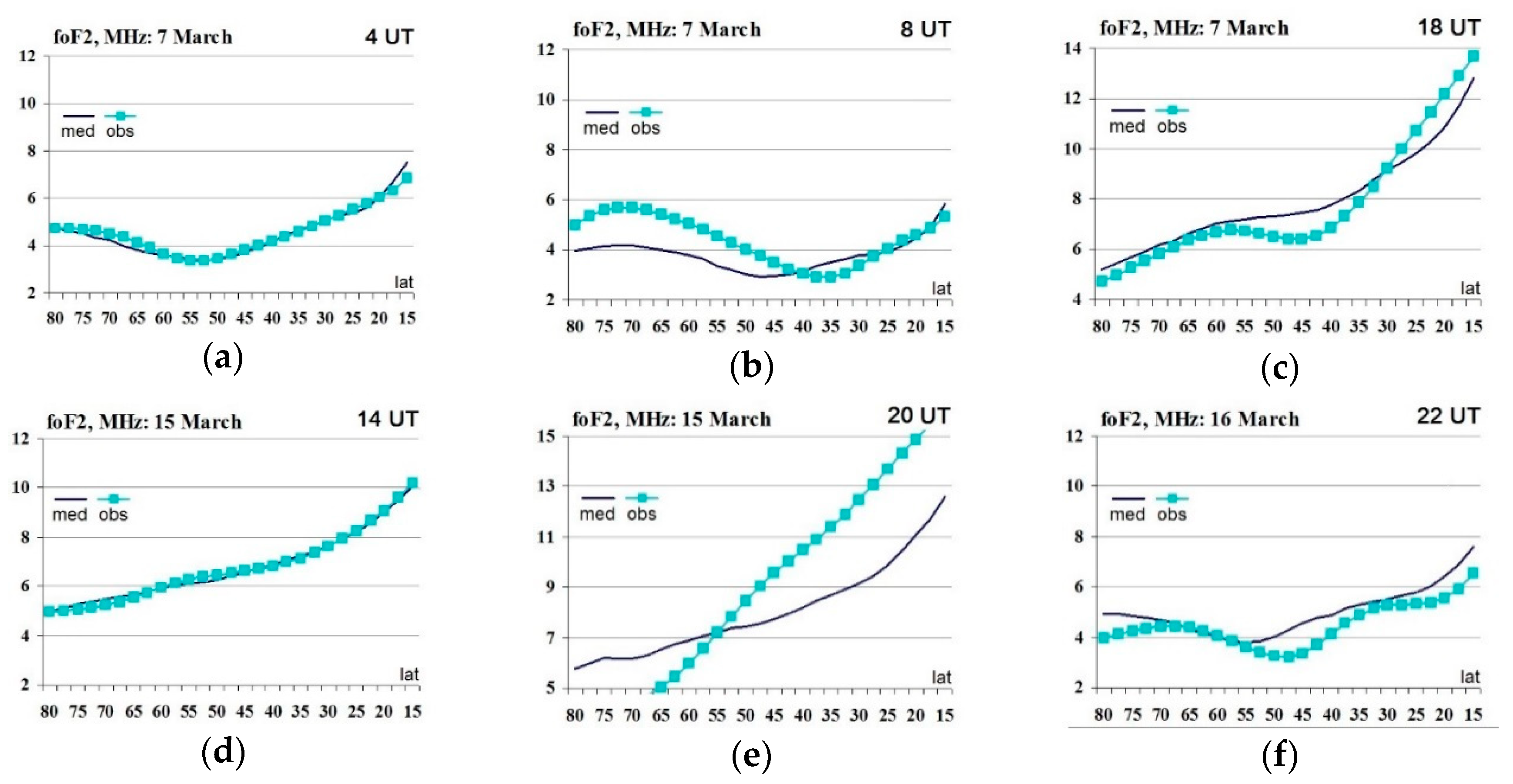
4.1. foF2 Response to the Storms during 7–17 March 2012

The general picture of foF2 changes is represented in Figure 10 and Figure 11. To give it a closer look, separate plots for each UT hour on each particular day (132 plots in total) were analyzed during 7–17 March 2012. Figure 12 provides their examples (analogous to those in Figure 10, but enlarged). The following features were revealed during storms №1–4.

Storm №1: foF2 responded about 2 h after the MP beginning with positive ionospheric disturbance at high-to-mid latitudes and negative at mid-to-low latitudes. This tendency changed 2 h after the RP beginning: A negative disturbance originated at low–mid latitudes and moved, with time, to higher latitudes, finally resulting in a complex disturbance picture along the longitudinal sector. The latitudinal structures of electron density distribution became more pronounced during ionospheric disturbance: MIT shifted southward during MP and the border of the EIA northern crest at mid latitudes became more sharp. The disturbance was mostly negative during the second half of RP with some positive deviations at high latitudes at the end (8 March 10–12 UT). The foF2 behavior after the end of RP was very close to its regular pattern along the meridian (from 8 March 14 UT). The high-latitude and mid–low-latitude behavior were always different during ionospheric perturbation caused by storm №1. The ionosphere returned to its quiet state after the storm.

Storm №2: The foF2 values before the disturbance were lower than usual at high latitudes. At the beginning of the storm, foF2 coincided with their quiet pattern. It seems that the response to the storm began to manifest itself about 5–6 h after the MP beginning and was characterized with positive foF2 deviations at high and mid latitudes (9 March 6 UT). The storm was characterized with the long RP beginning from 8 UT, since which the latitudinal structure of the electron density distribution was shifted to lower latitudes and the shape of this “structure” itself was more pronounced. The negative ionospheric disturbance developed during 12–22 UT covering all the latitudes. The less intense but still negative foF2 deviations dominated during 10 March with slight positive deviations at the particular hours within (20°–15°) N. During 16–22 UT, positive deviations were also observed within ~(60°–45°) N being the part of the more prominent MIT than usually at these hours. During 2–14 UT on 11 March, the ionosphere followed its quiet patterns of variation at all considered latitudes. RP ended at ~15 UT. Still, after this hour the latitudinal structure of electron density was more pronounced than during quiet periods. This was because the geomagnetic field was again moderately perturbed (Dst = −50 nT). At this background, the next disturbance developed.

Storm №3: MP lasted within 10–16 UT on 12 March. It resulted in the positive ionospheric disturbance within (40°-15°) N during 12–16 UT (2 h after the MP beginning) and was followed by the negative disturbance within (80°-45°) N during 16–18 UT (RP). The curves of the observed and median foF2 values almost coincide at 20 UT. The slightly negative foF2 deviations prevailed during 0–10 UT on 13 March along the whole meridian. Then, the very weak positive deviations became moderate along almost all latitudes except (80°–65°) N within 12–22 UT. To note, storm’s RP ended at 18 UT. After 22 UT, the foF2 behavior was close to its quiet patterns at all latitudes with some exceptions on the next day which are probably explained by the geomagnetic background that still was not quiet (Dst ~ −40 nT during the whole day).

Storm №4: Anyway, just before the next storm’s MP beginning (15 March 14 UT) the ionosphere showed the very quiet behavior during several hours. Again, the ionospheric response to the storm began 2 h after the MP beginning. During 16–22 UT, the very intense positive foF2 disturbance developed within ~(55°–15°) N and very intense negative disturbance within ~(80°–55°) N. RP began at 20 UT and its main part lasted approximately until 2 UT. During 16 March within 0–4 UT, there were observed the slightly decreased foF2 values along the meridian and generally more pronounced structure of latitudinal distribution of electron density. Except for the very high latitudes, foF2 during 6–10 UT coincided with its medians along the meridian. It can be concluded that the ionosphere quickly recovered as it did after the previous storms. Some Dst decrease occurred at 5 UT but then RP continued until ~14 UT. Again, the ionospheric response to Dst decrease was delayed. From 12 UT 16 March to 02 UT 17 March the mixed/complex ionospheric disturbances developed at different latitudes. During 20–02 UT, MIT manifested itself much more intense if compared to its median form.

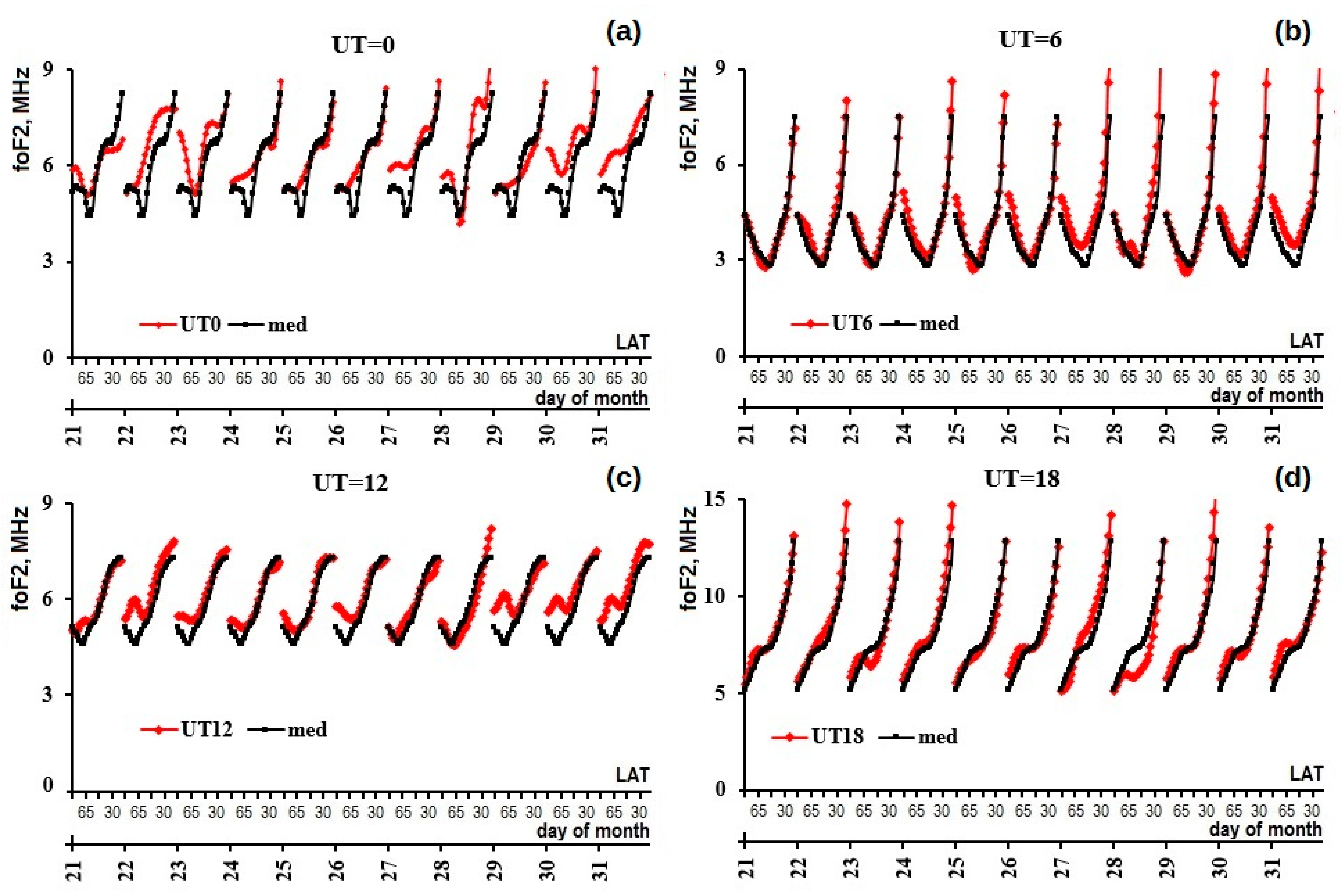
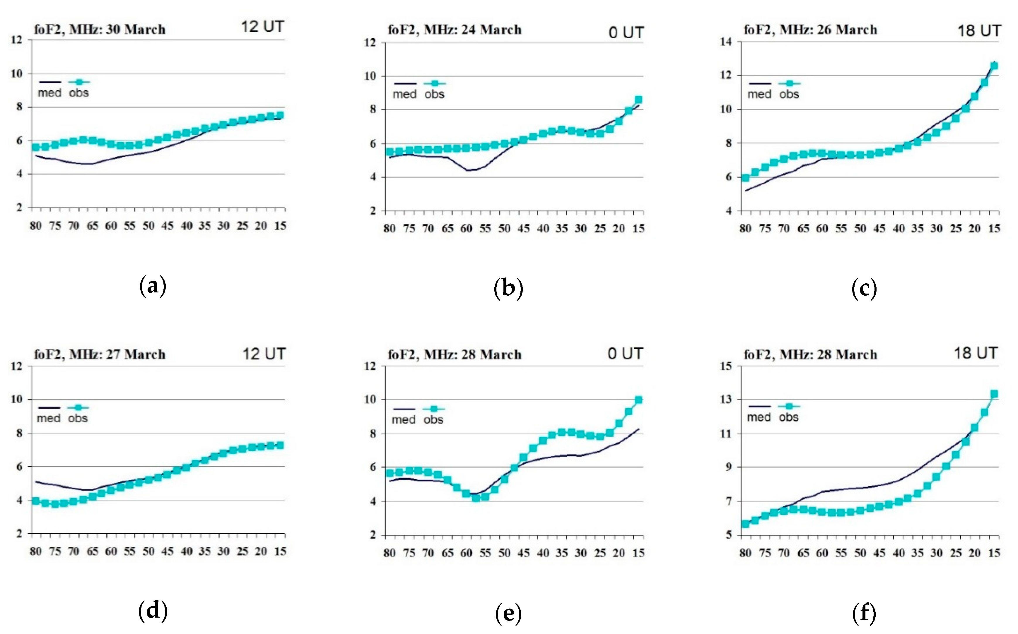
4.2. foF2 Response to the Storm during 21–31 March 2012

According to the experimental ionosonde data (discussed in Section 3.3), the period of 21–31 March was characterized with the generally enhanced foF2 during quiet geomagnetic days (control days). In contrast, during the storm foF2 was closer to its regular (median) pattern of variations except for the low-latitude station. A more detailed picture was obtained with foF2(rec): 132 separate plots during 21–31 March were constructed analogously to the period of 7–17 March.

Storm №5: At the moment of the storm’s MP beginning at 10 UT on 27 March, the foF2 was still similar to its value on the control days (days that preceded or followed the storm). As in the previous four cases, the foF2 behavior along the meridian changed 2 h after the MP beginning. During 12–14 UT, the negative foF2 deviations at high latitudes were observed (Figure 13d) instead of positive deviations on control days (Figure 13a). At other latitudes foF2 coincided with its medians. The density decrease at high latitudes remained during 16–18 UT. In addition, foF2 at other latitudes tended to differ from its values on the control days. The latitudinal structures like MIT were less pronounced than during the same hours of control days. At 20 UT, the foF2 deviations were mostly positive and more prominent and mid and low latitudes (in contrast of being close to its median patterns on control days); and at high latitudes, they coincided with medians (instead of being increased like on control days). At 22 UT, the slight increases at mid and low latitudes and the coincidence with median values at high latitudes were observed. On the control days, these variations were exactly the opposite: coincided with medians at mid and low latitudes and were positive at high latitudes.

0 UT means local evening conditions. Regularly, the latitudinal foF2 dependence changed significantly between 22 and 0 UT in March 2012: the curves of median values marked MIT appearance at 0 UT, which was absent at 22 UT of the previous day. This was because 22 UT (17 LT) was still on the lighted side of Earth and 0 UT (19 LT) was the hour when the solar terminator was passing or just had passed the ionospheric heights over the region. To note, during the control (non-storm) days the MIT structure was very smoothed or not observed: The foF2 was increased exactly over the MIT latitudes, instead of being much lower due to MIT presence. However, during the storm’s MP at 0 UT, the pronounced MIT was observed coinciding with its median pattern. As for mid and low latitudes, positive disturbances were observed there (Figure 13e), instead of quiet variations on control days (Figure 13b). The picture was similar at 2 UT (MP): MIT was more profound. In addition, the positive mid- and low-latitude disturbance arose, revealing the more structured latitudinal density distribution.

RP of the storm started at 04 UT on 28 March. During 4–6 UT, mid–low-latitudes strong positive foF2 disturbance and more latitudinal structures were observed. On control days, foF2 tended to follow its quiet pattern. During 8–10 UT, foF2s were close to their medians along the meridian in contrast to control days, when the high-latitude positive deviations occurred. Moreover, 12 UT was similar to control days. During 14–22 UT, the strong negative disturbance arose from 65° N towards mid latitudes, gradually covering low latitudes, as well. On control days (with one exception), the ionosphere during these hours tended to be quiet at mid and low latitudes and positively disturbed at high latitudes (Figure 13c), which again means the opposite behavior during control days and during the storm (Figure 13f). Moreover, foF2 at 0 UT on 29 March was the same as on control days. During 2–8 UT the values were close or coincided with their quiet medians again. RP ended approximately at 11 UT. Moreover, foF2 behavior was similar to its behavior on the control days from 10 UT and further.

To sum up, the following common ionospheric features were revealed during five storms.

(1)

The ionospheric responses to MP and RP of geomagnetic storms differed. The change in the ionospheric reaction was quite clear in four cases.

(2)

The ionosphere responded to the MP of each storm 2 h after its beginning (later in one case). It also changed its behavior ~2 h after the storm’s RP beginning in four cases (Figure 12a,d).

(3)

The ionosphere returned to its regular state rather quickly after each geomagnetic storm. Therefore, though the short period of 7–17 March was characterized by a series of geomagnetic disturbances, it was possible to distinguish the response to each particular storm.

(4)

The ionospheric structures such as MIT and the border of the northern crest of EIA were more prominent during all storms (higher electron density gradients) instead of being smoothed and sometimes shifted as on non-storm days. Sometimes they manifested themselves in much sharper forms and/or were shifted in latitude if compared to their quiet regular patterns. For instance, foF2 curves in Figure 12b,c,e,f.

(5)

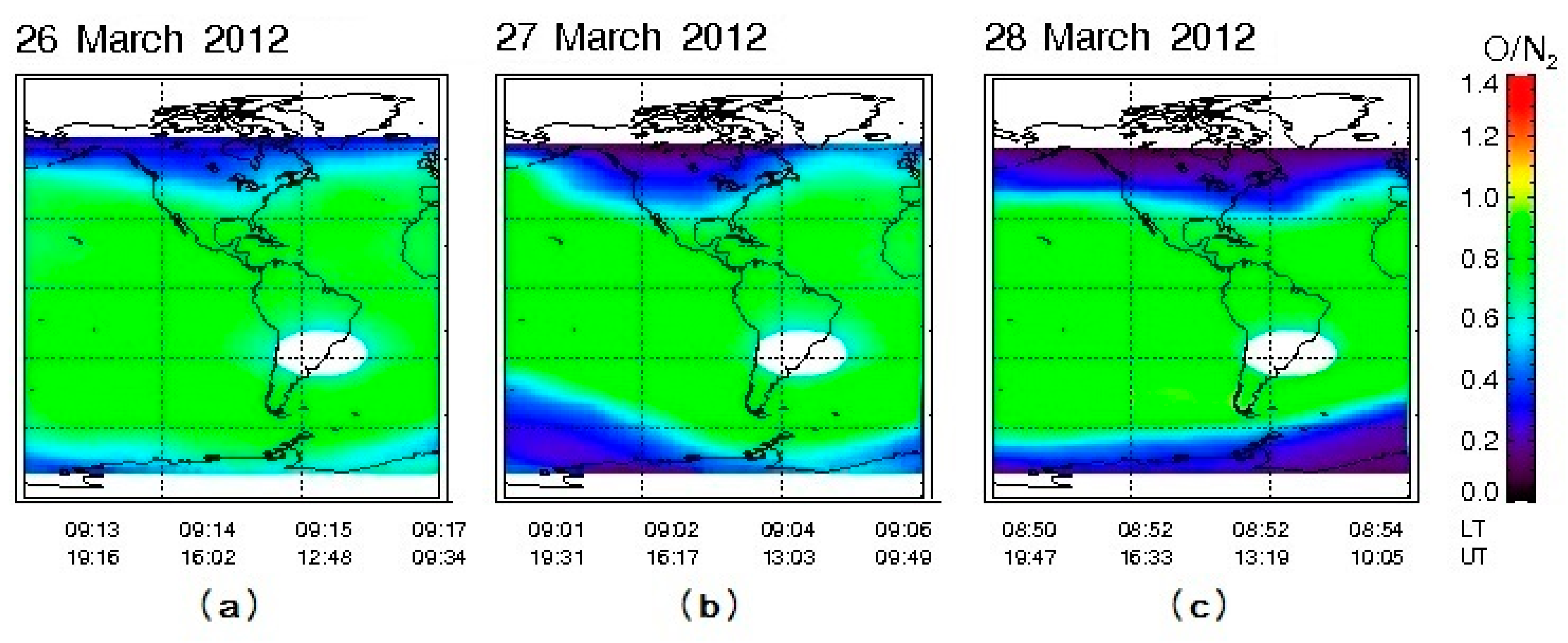
The response to storm №5 developed at an already non-quiet ionospheric background: foF2 values were increased under quiet geomagnetic conditions most of the time especially at high latitudes. During the storm, the foF2 values were exactly the opposite to these background variations: decreased at high latitudes instead of being increased and increased more intensively than during geomagnetically quiet days at lower latitudes. Eventually, this confirms the preliminary conclusion indicating that the ionospheric behavior was probably controlled by O/N₂ changes along the 70° W longitude due to geomagnetic storm impact.

5. Correlation between the Ionospheric and Space Weather Parameters

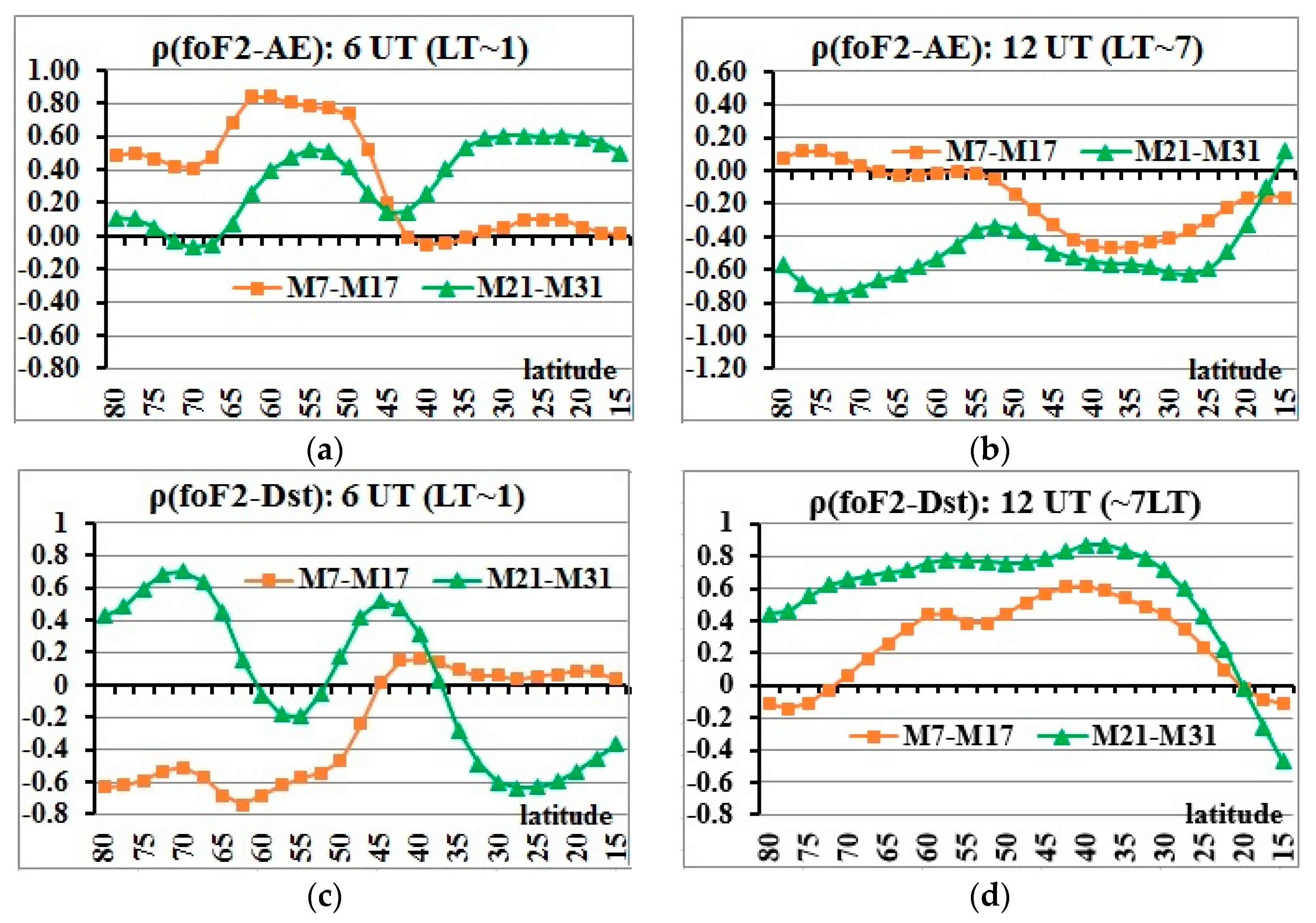
5.1. Paired Correlation Analysis

We tried to assess qualitatively the contribution of different Space Weather (SW) parameter changes to ionospheric processes during the considered geomagnetic disturbances. Since the paired correlation is the most common and simplest way for assessing correlations, the coefficients of linear correlation (ρ) were calculated between the foF2(rec) value at the particular hour and daily averaged value of a particular SW parameter. Figure 14 shows the examples. Such plots were constructed for foF2(rec) at 0, 6, 12 and 18 UT and all the parameters from Figure 2. The results showed the very complex correlation picture. The only revealed feature was that the impact of each SW parameter on foF2(rec) behavior depended significantly on the latitude of observations. Correlation tendencies for TEC were rather similar and confirmed this conclusion.

According to results for the particular hours, ρ between foF2(rec) and Dst was very different at different hours and latitudes, e.g., in Figure 14 (lower panels). We recall that the ionosphere responded to Dst disturbance with 2 h delay during four of five storms. Therefore, the correlation coefficient (r) between the time series of ∆foF2 at latitudes 77.5, 67.5, 42.5 and 17.5°N and Dst during two 11-day periods was calculated with 2 and 4 h shifts, as well as without any shift. The results for 7–17 March showed that at all latitudes the highest r was for 4 h delay of ∆foF2 series and the lowest r was without any delay. Moreover, r was the highest for 4 h, and not 2 h, delay because of the 5–6 h shift during the second storm that was the longest and most intense among other storms (Figure 2). The best correlation during 21–31 March was again for the 4 h delay of ∆foF2 series at all latitudes, except for the low latitude. In general, the dependence of ∆foF2 on Dst-index during the second 11-day period was stronger than during the first period.

The examples provided in Figure 14 and the results for other SW parameters (even more complex than for ∆foF2 and Dst) demonstrated that there is a certain relationship (rather strong at some latitudes) and at the same time a significant difference between different factors and periods. Obviously, the obtained high ρ/r values were due to the fact that other factors were not taken into account. Therefore, the following approach was applied.

5.2. Multiple Correlation Analysis

Obviously, none of the SW parameters acts independently. Changes of the ionosphere state is a result of a complex impact caused by the sum of near-Earth space phenomena. A multiple correlation analysis allows us to at least roughly assess the contribution level of one or another SW parameter in variations of ∆foF2 at different latitudes. The Principal Components Analysis (PCA) and the consequent principal component regression analysis (PCR) were performed. These are the widely used methods inclusive for the Space Weather tasks, for instance [46,47]. Their detailed mathematical description and definitions of terms can be found in References [48,49]. Here, we briefly mention the basic steps of the performed analysis, trying to explain what was done in a simple way.

(a)

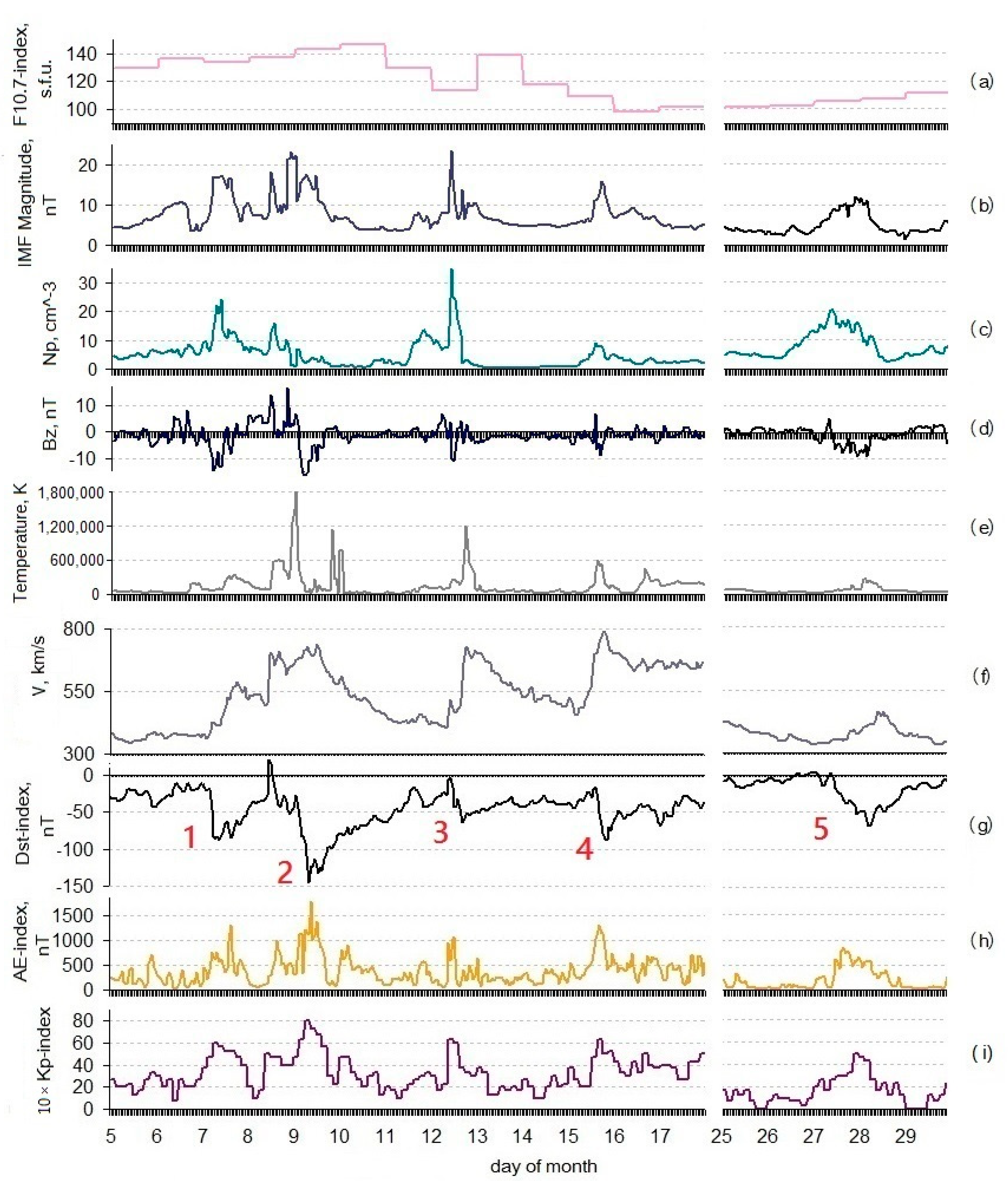
In our case, ∆foF2(rec) was considered as a “dependent” parameter (response variable) which was influenced by a set of SW parameters variations (explanatory variables). Considering the solar wind and interplanetary environment triggers of each geomagnetic storm discussed in Section 2 (Figure 2), we selected IMF, Bz, Np, V and AE to be included into the set of explanatory variables. F10.7-index was not involved as it characterizes the longer-term variations of solar activity than the considered 11-day periods. Dst-index was not involved because we already included AE; and Dst and AE variations were very similar which preferably should be avoided for explanatory variables in PCA. Thermospheric ratio O/N₂ played a significant role in the ionospheric behavior (see Section 3). Consequently, it was included in the explanatory variables set, but only for the analysis at high and mid latitudes. This is because the ratio almost did not change at low latitudes and there were too many gaps of GUVI/TIMED satellite data at very high latitudes.

(b)

Further, the data were standardized, which means transformation of data distribution into the new distribution with zero mean and single (unitary) standard deviation. This results in that all explanatory variables have the same statistical weight in order to highlight the variance contrast.

(c)

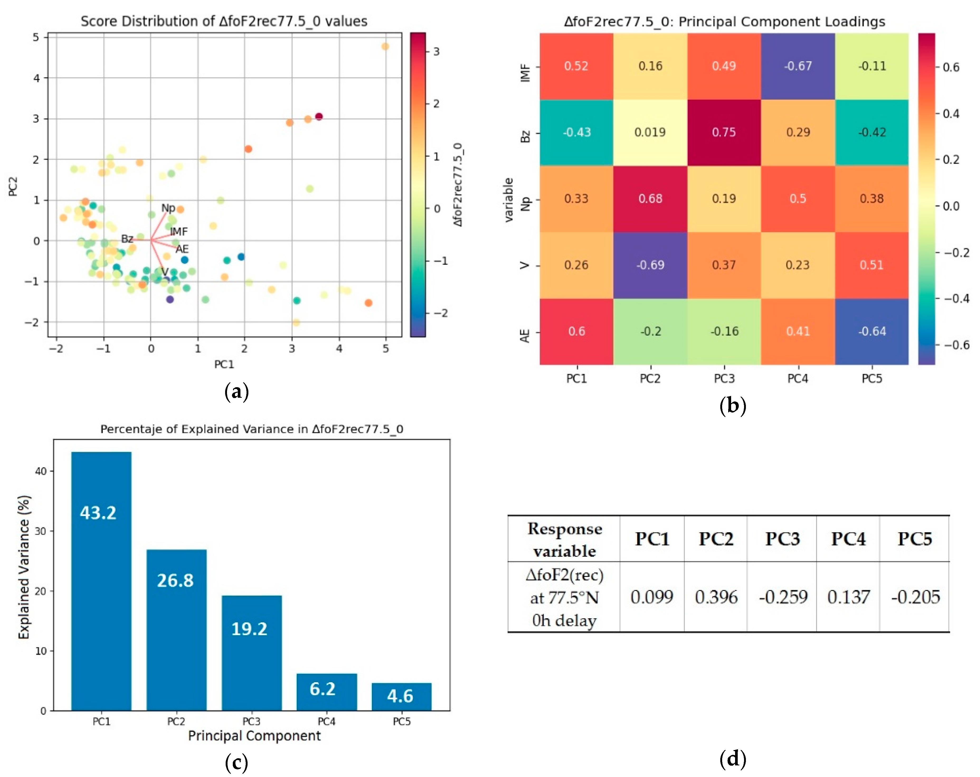
Then, the principal components (PCs) were calculated for this new dataset. Each PC is a linear combination of the uncorrelated original explanatory variables, which forms an eigenvector of the covariance–correlation matrix. The response variable can be expressed via PCs as follows:

∆foF2 = a × PC1 + b × PC2 + c × PC3 + d × PC4 + e × PC5 (+ f × PC6),

(5)

where a–f are the multivariate regression coefficients of response variable ∆foF2 in terms of PCs. Each PC is a multi-dimensional vector. Example is given in Figure 15a. Each plane corresponds to a particular original explanatory variable. As the data were standardized, ∆foF2 values are expected to be clustered in the directions of the original explanatory variables, which is what exactly seen in the plot. Each PC can be expressed as an intermix of the original variables. The following offers an example:

PC1 = L₁₁ × AE + L₁₂ × V + L₁₃ × Np + L₁₄ × Bz + L₁₅ × IMF (+ L₁₆ × O/N₂),

(6)

where L_ij are the loadings of PCi in terms of the original explanatory variables (IMF, Bz, Np, V and AE), or in other words, the correlation coefficients between IMF, Bz, Np, V, AE and PCs. Figure 15b shows the example of the covariance matrix containing the loadings for time series of ∆foF2 during 7–17 March 2012: Each column represents the loadings for a particular PC.

(d)

The scree plot is a graph that shows the magnitudes of the eigenvalues of the covariance–correlation matrix. For example, Figure 15c illustrates the level of each PC impact on the response variable (percentage of ∆foF2 variance explained by a particular PC). Usually, it is supposed that it is sufficient to consider the components that explain 85% of the response variable variations; and the components of minor influence may be neglected. Though three first PCs mostly explained more than 85% of ∆foF2 variations, we considered five components. This is because in our case the same original explanatory variable could contribute significantly to several PCs (for instance, IMF in PC1, PC3 and PC4 in Figure 15b) [50]. The analysis showed that the consideration of less than five components resulted in the false intensification or decrease of the role of such explanatory variables.

(e)

Formulae 5 and 6 describe the PCA decomposition and a consequent regression step represented by PCR. Preferably, the explanatory variables should be totally independent from each other. From the physical point of view, in our case they are not absolutely independent because eventually they represent different processes that define Space Weather conditions. That is why, the direct comparison of IMF, Bz, Np, V and AE contributions to PCs (values of their loadings in each column of the matrix) resulted in the confusing results meaning that PCA was not sufficient to draw the conclusions. To eliminate the multicollinearity between our explanatory variables, PCR [51] was performed which is basically an extension of PCA. In PCR analysis, instead of regression of the dependent ∆foF2(rec) on the explanatory variables directly, the principal components or eigenvectors (v) of their variance–covariance matrix coefficients of explanatory variables (Figure 15b) are used as regressors (Equation (6)). Typically, only a subset of all the principal components is used for regression, making PCR a kind of regularized procedure or shrinkage estimator. According to equation 6, the final regression coefficients were obtained by multiplying PC values calculated for ∆foF2(rec) by the corresponding loading values (Figure 15d). ∆foF2(rec) of the particular latitude and time delay from the storm beginning were analyzed separately.

(f)

Finally, the contribution of variations of each SW parameter on the ionospheric response was presented in the form of percentage of the “explained” variance of ∆foF2(rec), based on the regression coefficient values obtained in PCR. Considering the contribution of each parameter to a particular PC, the dominant contributions or, in other words, the factors that had a dominant influence on foF2 at the particular latitude can be qualitatively estimated.

To ensure the reliability of our calculations, the PCR and PCA algorithms used in this study were checked with a test dataset. It is also worth noting that, in general, the large dispersion of the data was observed, e.g., in Figure 15a. This means that the regression model should be probably not lineal. At the same time, the linear multiple regression allowed us to make the rough estimations given below.

First, a multiple linear correlation analysis described above was applied for the IMF, Bz, Np, V and AE time series during two 11-day periods (7–17 March and 21–31 March 2012) and the corresponding ∆foF2(rec) time series during the same periods calculated at four latitudes. It was shown above that the ionosphere responded with a delay of (2–5) h to geomagnetic storms caused by the perturbed SW conditions. Therefore, the analysis was performed for ∆foF2(rec) series that coincided in time with SW parameters variations (without any delay), for ∆foF2(rec) series shifted in time in 2 and 4 h, in regard to the SW parameters time series, to reveal which delay provides a better correlation.

Second, a multiple linear correlation analysis was performed for the daily averaged values of IMF, Bz, Np, V, AE and O/N₂ during 11 days and the corresponding day-to-day variation of foF2(rec) value at a particular UT hour. The daily averaged SW parameters values characterize the overall level of SW perturbation during the particular day.

5.2.1. 7–17 March 2012

Table 2. Main contributors to foF2(rec) at high latitudes (HL), mid latitudes (ML) and low latitudes (LL), along 70° W.

Ionospheric Response Delay	HL: 77.5° N	HL: 67.5° N	ML: 42.5° N	LL: 17.5° N
	(87.2° N)	(77.2° N)	(52.2° N)	(27.3° N)
0 h	V(40%)	V(35%)	IMF(37%)	AE(43%)
	Np(23%)	IMF(26%)	V(25%)	Bz(28%)
	AE(20%)	Np(23%)	AE(22%)	IMF(19%)
2 h	Bz(30%) V(27%) Np(23%)	V(44%) AE(19%) Np(18%)	IMF(49%) V(28%) Bz(21%)	AE(53%)
				IMF(18%)
				Bz(15%)
				Np(14%)
4 h	V(54%) Bz(29%)	V(42%)	AE(39%) Bz(30%)	AE(64%)
		AE(30%)		IMF(17%)
		IMF(13%)		V(17%)

shows the results of the analysis for the time-series. Each column stands for the particular geographical latitude; its corresponding geomagnetic latitude is given in brackets. It is clearly seen the latitudinal and temporal dependence of contributing processes predominantly responsible for the change of foF2 patterns during 7–17 March.

77.5° N (87.2° N) corresponds to the polar cap. Here, the solar wind speed played the dominant role. The Bz-component influence was also detected.

67.5° N (77.2° N) can be referred to the northern border of the auroral zone. At this latitude, the main role still belongs to the solar wind speed. Proton density, IMF magnitude and AE-index also had their word in the overall picture of foF2 variations.

42.5° N (52.2° N) refers to the mid-latitude zone. Here, a mixed influence was observed as well: different factor dominance at different hours. IMF magnitude role and some role of AE were emphasized.

17.5° N (27.3° N) refers to the low-middle latitudes in terms of geomagnetic coordinates. Although, in general, a mix of different impacts is seen, the dominant role of AE is clearly noted.

Probably in the last case, AE represents not only the auroral electrojet and auroral processes, but stands in as a general geomagnetic field variations measure. Indeed, even visually the behavior of AE and Dst in Figure 2 was very similar; and the negative correlation between the two indices was high during two considered periods (−(0.5–0.8)). Comparison of middle and lower panels of Figure 14 proves this fact. In Section 4.1, it was shown that foF2 responded to geomagnetic disturbances with a delay, and this is exactly what is seen from Table 2 (AE impact level grows with delay).

A multiple correlation analysis was also performed for 24 datasets formed of series of daily averaged SW parameters and ∆foF2(rec) at the particular UT hour.

Table 3. Main contributors to foF2(rec) at four latitudes estimated for different hours of the day.

Hour	HL: 77.5° N	HL: 67.5° N	ML: 42.5° N	LL: 17.5° N
	(87.2° N)	(77.2° N)	(52.2° N)	(27.3° N)
0 UT (~19 LT)	Np(38) IMF(34)	Np(35) V(32) IMF(30)	IMF(36) Bz(36) Np(20)	V(26)Np(23)Bz(22)AE(21)
		Np(30)V(27)IMF(23)O/N2(16) 1	IMF(37) Bz(32) O/N2(16) 1
6 UT (~1 LT)	IMF(35) V(25)	IMF(43) Np(31) V(19)	Np(34) Bz(32)	IMF(40)AE(32)V(20)
		IMF(39) Np(32) V(23) 1	Np(31) Bz(30) O/N2(26) 1
12 UT (~7 LT)	Bz(33)AE(28)V(28)	Bz(36) IMF(21)	Np(28)AE(23)V(23)IMF(19)	IMF(37)Np(34)
		Bz(34) IMF(22) 1	Np(28) O/N2(28) 1
18 UT (~13 LT)	Bz(33)Np(28)V(24)	Np(27) V(27)	Bz(41) IMF(30) AE(22)	Np(26)AE(24) V(22)
		O/N2(40) AE(35) 1	O/N2(39) AE(28) 1

¹ Variables include O/N₂.

shows the results. Correlation coefficients were calculated for the set of five explanatory variables at all four latitudes and for the set of six explanatory variables at two latitudes (given in italics).

The overall impression of the obtained results is that the picture of SW impacts was very complex. Sometimes it is difficult to determine a leading contribution. This circumstance implies a strong interaction of the triggering processes. It also means that there are factors that were not taken into account. First, let us consider the correlation results when five SW parameters were considered.

At 77.5° N (87.2° N) the Bz impact dependence on day/night conditions is noted. Solar wind speed played a notable role. This confirms the conclusions made for the time-series of parameters at this latitude. IMF magnitude impact manifested itself in the evening and night, and the proton density impact in the evening. AE impact is noted in the morning (~7LT). This is because three of the geomagnetic storms occurred within ~(5–9) LT.

At 67.5° N (77.2° N) again there was a difference between the most pronounced impacts at day and night. In general, a mixed influence of Np, V, IMF, Bz was observed. This is not exactly the conclusion that was made for the time series, but it coincides in that the impacts at this latitude were rather mixed (several factors participation).

At 42.5° N (52.2° N) a mixed influence, different at different hours, was observed. IMF magnitude impact dominated in the evening. AE played some role at night and morning hours which makes sense for this latitude. The influence of both factors was also revealed by the time-series correlation. The daily averaged data analysis showed also the prominent roles of Bz in the evening and night hours and proton density in the night and morning hours.

At 17.5° N (27.3° N) the impacts were rather mixed. IMF magnitude played a significant role at night and morning hours.

Furthermore, the analysis that involved six SW parameters was performed for two latitudes and showed the following. Except for the daytime hour 18 UT (~13LT), the dominant factors did not change when comparing to the results for five involved SW parameters. At the same time the role of O/N₂ variations became clear. It was most pronounced at mid latitudes. It is logical because the main changes of the thermospheric composition during geomagnetic storms occurred near this latitude in the considered sector. At mid latitudes, O/N₂ impact was observed at all hours, being the lowest at the evening and the highest under the daytime conditions. At high latitudes, O/N₂ played a leading role during the daytime with a tendency of slight decrease in the evening.

To sum up, the solar wind speed played the dominant role at high and very high latitudes. The Bz-component impact presence at very high latitudes depended on day/night conditions. At high, mid and low latitudes, the impacts of several phenomena were combined and showed their dependence on day/night conditions. This is probably because geomagnetic storms within 7–17 March were triggered by different processes. Thermospheric ratio manifested its impact constantly at mid latitudes. This impact dominated the daytime ionosphere of mid and high latitudes.

5.2.2. 21–31 March 2012

Analogously to the previous section the analysis was performed for the 11-day time-series and for the variables’ daily averaged values.

Table 4. The same as in Table 2 but for 21–31 March 2012.

Ionospheric Response Delay	HL: 77.5° N	HL: 67.5° N	ML: 42.5° N	LL: 17.5° N
	(87.2° N)	(77.2° N)	(52.2° N)	(27.3° N)
0 h	Bz(54%) V(27%)	Bz(27%) IMF(26%) V(23%) AE(16%)	IMF(50%) V(26%) Np(18%)	AE(36%) Bz(23%)
2 h	AE(52%) V(30%)	AE(35%) IMF(27%) V(26%)	V(38%) IMF(34%)	AE(42%) V(32%)
4 h	AE(55%)	AE(37%) V(26%) IMF(24%)	V(29%) Bz(21%) IMF(20%)	AE(36%) V(31%)

and

Table 5. The same as in Table 3 but for 21–31 March 2012.

Hour	HL: 77.5° N	HL: 67.5° N	ML: 42.5° N	LL: 17.5° N
	(87.2° N)	(77.2° N)	(52.2° N)	(27.3° N)
0 UT (~19 LT)	Bz(44) AE(31)	IMF(39) AE(22) Bz(19)	AE(34) IMF(32) Bz(20)	AE(44) Bz(26)
		AE(33) Bz(27) 1	AE(39) Bz(26) 1
6 UT (~1 LT)	AE(37) Np(30)	AE(42) Bz(24) IMF(21)	AE(42) Bz(26) IMF(24)	AE(38) Np(32)
		AE(43) Bz(26) IMF(20) 1	AE(41) Bz(27) 1
12 UT (~7 LT)	AE(35) Bz(35) IMF(21)	AE(46) IMF(19) Bz(18)	AE(45) Bz(20) IMF(18)	Np(32)IMF(25)Bz(24)
		AE(31) Bz(31) 1	AE(45) Bz(20) 1
18 UT (~13 LT)	Bz(49)Np(18)AE(16)IMF(16)	AE(63)	AE(42) Bz(25)	Bz(32)AE(30)IMF(19)
		AE(63) 1	O/N2(28)Np(26)AE(22) 1

¹ Variables include O/N₂.

represent the results. In general, this period was characterized with the dominance of one or two SW parameters in contrast to the mixed picture of 7–17 March.

According to Table 4, at 77.5° N (87.2° N), there was a clear immediate dominance of Bz-component variations on the foF2 change. The solar wind speed change affected the ionosphere of the polar cap significantly, as well. The AE bursts impact was delayed but intense.

At 67.5° N (77.2° N), similarly to the higher latitude, Bz and solar wind speed were important immediate impacts. In addition, IMF magnitude was of the same level of importance. AE bursts impact was delayed as at the higher latitude.

At 42.5° N (52.2° N), the IMF magnitude impact was immediate. The role of solar wind speed was also important though a bit delayed. Other SW parameters also manifested themselves.

At 17.5° N (27.3° N), the dominant parameter was AE. The explanation is the same as for 7–17 March. The best correlation is for the 2 h delay. Indeed, as discussed in Section 4, the ionosphere response was delayed 2 h from Dst decrease during storm №5. The solar wind speed impact was delayed and the same level of Bz impact was immediate.

According to Table 5, it can be assumed that, at 77.5° N (87.2° N), generally, AE and Bz dominated.

At 67.5° N (77.2° N), a clear dominance of the AE-index variations was detected which is explained by the fact that the latitude is near the northern border of the auroral zone. IMF magnitude had an immediate impact.

At 42.5° N (52.2° N), AE also played the main role. The second role clearly belonged to Bz. IMF magnitude had an immediate impact as at the higher latitude. The role of thermospheric ratio was the main at this latitude at 18 UT (daytime conditions). To note, storm №5 began at 10 UT, therefore the induced impact of O/N₂ was delayed. It may seem surprising that the O/N₂ role is less emphasized during the analyzed period than it seemed from observations discussed in Section 3. This is because 21–31 March included only two storm days; and, in general, under quiet geomagnetic conditions, O/N₂ variations did not have such impact on foF2 as during the storm.

At 17.5° N (27.3° N), geomagnetic field variations (represented by AE) impact was dominant under night conditions. The complex impact was observed under daytime conditions.

To sum up, during the second considered period, the role of geomagnetic field changes was dominant at all times of the day, at all latitudes, with few exceptions. At high latitudes, foF2 responded immediately to Bz variations, and with a delay to the solar wind speed change. This is not surprising, as storm №5 was provoked by the southern Bz-component associated with the transit of a streams interacting region caused by the coronal hole (see Section 2). Thermospheric ratio controlled the foF2 variations at mid latitudes, under daytime conditions.

To conclude, two 11-day periods differed significantly. In addition, it is clear that the ignoring of O/N₂ variations in the considered latitudinal sector during geomagnetic disturbances would lead to incorrect conclusions.

6. Conclusions

This study discusses the features of ionospheric disturbances within the longitudinal sector of the Northern Hemisphere along the meridian of 70°W. The analyzed disturbances were caused by five magnetic storms of different intensity triggered by different Space Weather phenomena in March 2012. The state of the ionosphere was diagnosed with TEC and foF2 data.

The use of latitudinal dependence of the experimental monthly median value of the equivalent slab thickness of the ionosphere for reconstruction of lacking foF2 values in the considered region proved its effectiveness and allowed us to study the latitudinal features along the meridian in detail. For the ionospheric slab thickness estimation, the experimental ionosonde data from four ionospheric stations and GIM TEC data were used.

The following results were obtained:

• Latitudinal dependence of the median value of the ionospheric slab thickness was obtained with use of polynomial approximation. The polynomial of third degree provided the confidence factor close to 1 for all UT hours except 12 UT (~7 LT), when the linear approximation with the confidence factor of 0.98 was sufficient.
• The synchronicity of changes of experimental TEC and foF2 values (changes of their behavior) was shown by data of four ionosondes during disturbances.
• The suggested method of construction of τ(med) latitudinal dependence applied to the analysis of foF2 during the disturbances of March 2012 allowed us to reveal the latitudinal features, which generally confirm the results of studies of such variations performed for local regions or for separated magnetic storms. In particular, (a) MIT structure and the border of the EIA northern crest manifested themselves in the much sharper and prominent forms and/or were shifted in latitude during all storms (higher electron density gradients). (b) Ionospheric response was delayed by 2 h from the storm’s beginning, in most cases (by 5–6 h in one case). The responses to the main and recovery phases in most cases was different. (c) The response to the storm of 27–28 March developed at an already non-quiet ionospheric background and was controlled by O/N₂ changes due to geomagnetic storm impact.
• A qualitative assessment of the differences in the degree of influence of SW parameters variations on the ionosphere of different latitudes for two periods was obtained. The results of multiple correlation analysis for 7–17 March and 21–31 March differed significantly, but in both cases, during the geomagnetic disturbances, O/N₂ variations in the considered longitudinal sector played a significant role in the ionospheric state change at mid latitudes. During the first period, the solar wind speed played the dominant role at high and very high latitudes. At high, mid and low latitudes, the impacts of several phenomena were difficult to separate. This combination of impacts depended on day/night conditions. During the second period, the geomagnetic storm developed on the quiet geomagnetic background, and the role of geomagnetic field changes was dominant.

References

- Cannon, P. Extreme Space Weather: Impacts on Engineered Systems and Infrastructure. Report; Royal Academy of Engineering, Prince Philip House: London, UK, 2013; Available online: www.raeng.org.uk/spaceweather (accessed on 19 November 2020).
- Goodman, J.M. Operational communication systems and relationships to the ionosphere and space weather. Adv. Space Res. 2005, 36, 2241–2252. [Google Scholar] [CrossRef]
- Klimenko, M.; Klimenko, V.; Zakharenkova, I.; Ratovsky, K.; Korenkova, N.A.; Yasyukevich, Y.; Mylnikova, A.; Cherniak, I. Similarity and differences in morphology and mechanisms of the foF2 and TEC disturbances during the geomagnetic storms on 26–30 September 2011. Ann. Geophys. 2017, 35, 923–938. [Google Scholar] [CrossRef]
- Jin, H.; Maruyama, T. Different behaviors of TEC and NmF2 observed during large geomagnetic storms. J. Int. Nat. Inst. Info. Comm. 2009, 56, 369–376. [Google Scholar]
- Cander, L.R.; Ciraolo, L. Ionospheric total electron content and critical frequencies over Europe at solar minimum. Acta Geophys. 2010, 58, 468–490. [Google Scholar] [CrossRef]
- Chen, P.; Liu, H.; Ma, Y.; Zheng, N. Accuracy and consistency of different global ionospheric maps released by IGS ionosphere associate analysis centers. Adv. Space Res. 2020, 65, 163–174. [Google Scholar] [CrossRef]
- Khattatov, B.; Murphy, M.; Gnedin, M.; Sheffel, J.; Adams, J.; Cruickshank, B.; Yudin, V.; Fuller-Rowell, T.; Retterer, J. Ionospheric nowcasting via assimilation of GPS measurements of ionospheric electron content in a global physics-based time-dependent model. Q. J. R. Meteorol. Soc. 2005, 131, 3543–3559. [Google Scholar] [CrossRef]
- Davis, K.; Liu, X.M. Ionospheric slab thickness in middle and low latitudes. Radio Sci. 1991, 26, 997–1005. [Google Scholar] [CrossRef]
- Jakowski, N.; Stankov, S.; Wilken, V.; Borries, C.; Altadill, D.; Chum, J.; Buresova, D.; Boska, J.; Sauli, P.; Hruska, F.; et al. Ionospheric behavior over Europe during the solar eclipse of 3 October 2005. J. Atmos. Solar-Terr. Phys. 2008, 70, 836–853. [Google Scholar] [CrossRef]
- Huang, H.; Liu, L.; Chen, Y.; Le, H.; Wan, W. A global picture of ionospheric slab thickness derived from GIM TEC and COSMIC radio occultation observations. J. Geophys. Res. Space Phys. 2016, 121, 867–880. [Google Scholar] [CrossRef]
- Jayachandran, B.; Krishnankutty, T.N.; Gulyaeva, T.L. Climatology of ionospheric slab thickness. Ann. Geophys. 2004, 22, 25–33. [Google Scholar] [CrossRef]
- Fox, M.W.; Mendillo, M.; Klobuchar, J.A. Ionospheric equivalent slab thickness and its modeling applications. Radio Sci. 1991, 26, 429–438. [Google Scholar] [CrossRef]
- Bhonsle, R.; Da Rosa, A.; Garriott, O. Measurements of the total electron content and the equivalent slab thickness of the midlatitude ionosphere. Radio Sci. J. Res. 1965, 69D, 929–937. [Google Scholar] [CrossRef]
- Kenpankho, P.; Supnithi, P.; Tsuqawa, T.; Maruyama, T. Variation of ionospheric slab thickness observations at Chumphon equatorial magnetic location. Earth Planets Space 2011, 63, 359–364. [Google Scholar] [CrossRef][Green Version]
- Gerzen, T.; Jakowski, N.; Wilken, V.; Hoque, M.M. Reconstruction of F2 layer peak electron density based on operational vertical total electron content maps. Ann. Geophys. 2013, 31, 1241–1249. [Google Scholar] [CrossRef][Green Version]
- Roger, R. Measurements of the equivalent slab thickness of the daytime ionosphere. J. Atmos. Terr. Phys. 1964, 26, 475–497. [Google Scholar] [CrossRef]
- Sergeeva, M.A.; Maltseva, O.A.; Gonzalez-Esparza, J.A.; De La Luz, V.; Corona-Romero, P. Estimates of ionosphere state over Mexico with TEC data. In Proceedings of the 2017 XXXIInd General Assembly and Scientific Symposium of the International Union of Radio Science (URSI GASS), Montreal, QC, Canada, 19–26 August 2017; pp. 1–3. [Google Scholar] [CrossRef]
- Maltseva, O.; Mozhaeva, N.; Poltavsky, O.; Zhbankov, G. Use of TEC global maps and the IRI model to study ionospheric response to geomagnetic disturbances. Adv. Space Res. 2012, 49, 1076–1087. [Google Scholar] [CrossRef]
- Matamba, T.M.; Habarulema, J.B.; McKinnell, L.-A. Statistical analysis of the ionospheric response during geomagnetic storm conditions over South Africa using ionosonde and GPS data. Space Weather 2015, 13, 536–547. [Google Scholar] [CrossRef]
- Piersanti, M.; Cesaroni, C.; Spogli, L.; Alberti, T. Does TEC react to a sudden impulse as a whole? The 2015 Saint Patrick’s day storm event. Adv. Space Res. 2017, 60, 1807–1816. [Google Scholar] [CrossRef]
- Lekshmi, D.V.; Balan, N.; Ram, S.T.; Liu, J.Y. Statistics of geomagnetic storms and ionospheric storms at low and mid latitudes in two solar cycles. J. Geophys. Res. Space Phys. 2011, 116. [Google Scholar] [CrossRef]
- Ratovsky, K.; Klimenko, M.; Yasyukevich, Y.V.; Klimenko, V.; Vesnin, A.M. Statistical analysis and interpretation of high-, mid- and low-latitude responses in regional electron content to geomagnetic storms. Atmosphere 2020, 11, 1308. [Google Scholar] [CrossRef]
- Tsurutani, B.T.; Echer, E.; Shibata, K.; Verkhoglyadova, O.P.; Mannucci, A.J.; Gonzalez, W.D.; Kozyra, J.U.; Pätzold, M. The interplanetary causes of geomagnetic activity during the 7–17 March 2012 interval: A CAWSES II overview. J. Space Weather Space Clim. 2014, 4, A02. [Google Scholar] [CrossRef]
- Prikryl, P.; Ghoddousi-Fard, R.; Thomas, E.G.; Ruohoniemi, J.M.; Shepherd, S.G.; Jayachandran, P.T.; Danskin, D.W.; Spanswick, E.; Zhang, Y.L.; Jiao, Y.; et al. GPS phase scintillation at high latitudes during geomagnetic storms of 7–17 March 2012—Part 1: The North American sector. Ann. Geophys. 2015, 33, 637–656. [Google Scholar] [CrossRef]
- Reinisch, B.W.; Galkin, I.A. Global Ionospheric Radio Observatory (GIRO). Earth Planets Space 2011, 63, 377–381. [Google Scholar] [CrossRef]
- Mannucci, A.J.; Wilson, B.D.; Yuan, D.N.; Ho, C.H.; Lindqwister, U.J.; Runge, T.F. A global mapping technique for GPS-derived ionospheric total electron content measurements. Radio Sci. 1998, 33, 565–582. [Google Scholar] [CrossRef]
- Sugiura, M. Hourly Values of Equatorial Dst for the IGY; Annals of the International Geophysical Year 35; Pergamon Press: Oxford, UK, 1964; p. 9. [Google Scholar]
- Sugiura, M.; Kamei, T. Equatorial Dst Index 1957–1986; IAGA Bulletins 40; IUGG: Paris, France, 1991. [Google Scholar]
- Davis, T.N.; Sugiura, M. Auroral electrojet activity index AE and its universal time variations. J. Geophys. Res. 1966, 71, 785–801. [Google Scholar] [CrossRef]
- Bartels, J. The standardized Index Ks and the Planetary Index Kp; IATME Bulletin 12b; IUGG Publ.: Potsdam, Germany, 1949. [Google Scholar]
- Bartels, J.; Veldkamp, J. International data on magnetic disturbances, fourth quarter. J. Geophys. Res. 1954, 59, 297–302. [Google Scholar] [CrossRef]
- Bartels, J. The geomagnetic measures for the time-variations of solar corpuscular radiation, described for use in correlation studies in other geophysical fields. Ann. Int. Geophys. Year 1957, 4, 227–236. [Google Scholar]
- Richardson, I.G.; Cane, H.V. Near-earth interplanetary coronal mass ejections during solar cycle 23 (1996–2009): Catalog and summary of properties. Sol. Phys. 2010, 264, 189–237. [Google Scholar] [CrossRef]
- Yashiro, S.; Gopalswamy, N.; Michalek, G.; Cyr, O.C.S.; Plunkett, S.P.; Rich, N.B.; Howard, R.A. A catalog of white light coronal mass ejections observed by the SOHO spacecraft. J. Geophys. Res. 2004, 109. [Google Scholar] [CrossRef]
- Gopalswamy, N.; Yashiro, S.; Michalek, G.; Stenborg, G.; Vourlidas, A.; Freeland, S.; Howard, R.A. The SOHO/LASCO CME Catalog. Earth Moon Planets 2009, 104, 295–313. [Google Scholar] [CrossRef]
- Robbrecht, E.; Berghmans, D. Automated recognition of coronal mass ejections (CMEs) in near-real-time data. Astron. Astrophys. 2004, 425, 1097–1106. [Google Scholar] [CrossRef]
- Olmedo, O.; Zhang, J.; Wechsler, H.; Poland, A.; Borne, K. Automatic detection and tracking of coronal mass ejections in coronagraph time series. Sol. Phys. 2008, 248, 485–499. [Google Scholar] [CrossRef]
- Garton, T.M.; Gallagher, P.T.; Murray, S.A. Automated coronal hole identification via multi-thermal intensity segmentation. J. Space Weather Space Clim. 2018, 8, A02. [Google Scholar] [CrossRef]
- Zurbuchen, T.H.; Richardson, I.G. In-situ solar wind and magnetic field signatures of interplanetary coronal mass ejections. Space Sci. Rev. 2006, 123, 31–43. [Google Scholar] [CrossRef]
- Piersanti, M.; Alberti, T.; Bemporad, A.; Berrilli, F.; Bruno, R.; Capparelli, V.; Carbone, V.; Cesaroni, C.; Consolini, G.; Cristaldi, A.; et al. Comprehensive analysis of the geoeffective solar event of 21 June 2015: Effects on the magnetosphere, plasmasphere, and ionosphere systems. Sol. Phys. 2017, 292, 169. [Google Scholar] [CrossRef]
- Piersanti, M.; De Michelis, P.; Del Moro, D.; Tozzi, R.; Pezzopane, M.; Consolini, G.; Marcucci, M.F.; Laurenza, M.; Di Matteo, S.; Pignalberi, A.; et al. From the Sun to Earth: Effects of the 25 August 2018 geomagnetic storm. Ann. Geophys. 2020, 38, 703–724. [Google Scholar] [CrossRef]
- Stankov, S.M.; Warnant, R. Ionospheric slab thickness—Analysis, modelling and monitoring. Adv. Space Res. 2009, 44, 1295–1303. [Google Scholar] [CrossRef]
- Shinbori, A.; Otsuka, Y.; Tsugawa, T.; Nishioka, M.; Kumamoto, A.; Tsuchiya, F.; Matsuda, S.; Kasahara, Y.; Matsuoka, A.; Ruohoniemi, J.M.; et al. Temporal and spatial variations of storm time midlatitude ionospheric trough based on global GNSS-TEC and arase satellite observations. Geophys. Res. Lett. 2018, 45, 7362–7370. [Google Scholar] [CrossRef]
- Afraimovich, E.L.; Perevalova, N.P. GPS Monitoring of Earth Upper Atmosphere; Russian Academy of Sciences Siberian Branch: Irkutsk, Russia, 2006; pp. 1–460. ISBN 5-98277-033-7. [Google Scholar]
- Danilov, A. Ionospheric F-region response to geomagnetic disturbances. Adv. Space Res. 2013, 52, 343–366. [Google Scholar] [CrossRef]
- Krause, L.H.; Franz, A.; Stevenson, A. On the application of Exploratory Data Analysis for characterization of space weather data sets. Adv. Space Res. 2011, 47, 2199–2209. [Google Scholar] [CrossRef]
- Cadavid, A.C.; Lawrence, J.K.; Ruzmaikin, A. Principal components and independent component analysis of solar and space data. Sol. Phys. 2007, 248, 247–261. [Google Scholar] [CrossRef][Green Version]
- Pearson, K.F.R.S. LIII. On lines and planes of closest fit to systems of points in space. Lond. Edinb. Dublin Philos. Mag. J. Sci. 1901, 2, 559–572. [Google Scholar] [CrossRef]
- Hotelling, H. Analysis of a complex of statistical variables into principal components. J. Educ. Psychol. 1933, 24, 417–520. [Google Scholar] [CrossRef]
- Jolliffe, I.T. A note on the use of principal components in regression. J. R. Stat. Soc. Ser. C (Appl. Stat.) 1982, 31, 300–303. [Google Scholar] [CrossRef]
- Park, S.H. Collinearity and optimal restrictions on regression parameters for estimating responses. Technometrics 1981, 23, 289–295. [Google Scholar] [CrossRef]