Flattening of the Density Spectrum in Compressible Hall-MHD Simulations

Abstract

Observations of proton density fluctuations of the solar wind at 1 au have shown the presence of a decade-long transition region of the density spectrum above sub-ion scales, characterized by a flattening of the spectral slope. We use the proton density fluctuations data collected by the BMSW instrument on-board the Spektr-R satellite in order to delimit the plasma parameters under which the transition region can be observed. Under similar plasma conditions to those in observations, we carry out 3D compressible magnetohydrodynamics (MHD) and Hall-MHD numerical simulations and find that Hall physics is necessary to generate the transition region. The analysis of the k$\omega$ power spectrum in the Hall-MHD simulation indicates that the flattening of the density spectrum is associated with fluctuations having frequencies smaller than the ion cyclotron frequency.

1. Introduction

Solar Wind is a weakly collisional plasma whose proximity and variety of conditions make it an ideal environment to study plasma turbulence. In situ measurements of magnetic fluctuations in the solar wind provide a well-defined picture of the magnetic field spectrum along a large range of frequencies. Observations revealed that the magnetic spectrum is composed of multiple spectral slopes, each of which corresponding to a particular frequency range (e.g., Kiyani et al. [1], Chen [2]).

At 1 au and for frequencies smaller than the proton gyro-frequency (the so-called inertial range) the spectral index takes values between $-3/2$ and $-5/3$ (Podesta et al. [3], Chen et al. [4]). The spectrum is then followed by a short transition to a steeper slope around the proton gyro-frequency, with values between $-2$ and $-4$ (Smith et al. [5], Chen et al. [6], Franci et al. [7], submitted). Such slope continues until the electron gyro-frequency. At even higher frequencies, the existence of a power law in this range is still a source of discussion (Alexandrova et al. [8], Sahraoui et al. [9], Sahraoui et al. [10], Alexandrova et al. [11]).

Spectra of the proton density fluctuations have features similar to the magnetic ones, but the spectra flatten before the proton gyro-frequency is reached. The flattened region typically extends up to 1 decade above sub-proton scales. It has a spectral index between $-0.7$ and $-1.1$ and can be observed even when the magnetic and velocity spectra do not flatten (Chen et al. [12], Šafránková et al. [13] Šafránková et al. [14], Roberts et al. [15]).

One possible mechanism that could explain the formation of this transition region in the density spectrum is the presence of coherent structures. Pressure-balanced structures (PBS) are non-propagating structures that can be advected by the solar wind and are characterized by a constant total pressure (Tu and Marsch [16], Klein et al. [17], Verscharen et al. [18]). Their presence increases the intermittency of turbulence and alters the spectral slope close to ion inertial length scales, similarly to other coherent structures (Perrone et al. [19]).

Alternatively to PBS, Nearly Incompressible MHD (NI-MHD) theory provides a different way to model the solar wind density spectrum. In NI-MHD theory, fluctuations are expanded in powers of the small turbulent Mach number (Matthaeus et al. [20], Zank and Matthaeus [21]). In this framework, leading order density fluctuations were found to behave as a passive scalar of the magnetic fluctuations, while higher order corrections had a non-negligible effect only for fast timescales and short-length scales (Hunana and Zank [22]). For large Schmidt number (ratio of kinematic viscosity and passive scalar diffusivity), Hunana and Zank [23] described the passive scalar density spectrum as a double slope spectrum, that is, a Kolmogorov inertial range followed up by a viscous-convective range with a $k^{-1}$ scaling.

Chandran et al. [24] argued that, above sub-proton scales and close to the ion inertial length, density fluctuations associated to Kinetic Alfvén Waves (KAWs) can also contribute to the formation of the density spectrum. When Alfvén waves approach the ion inertial range, they transition into KAWs, becoming compressive modes. Linear theory predicts density fluctuations associated to KAWs are $k_{\perp }$ times proportional to perpendicular velocity fluctuations for KAW in the limit of small wave numbers (Hollweg [25]). Assuming that the spectrum of velocity fluctuations is $k_{\perp }^{-5/3}$ above sub-proton scales, the previous relation implies that the density spectrum generated by KAW density fluctuations should be $k_{\perp }^{1/3}$. This prediction for KAW density fluctuations is made for a range of scales, near and above the inertial length, where the presence of KAW modes is still sub-dominant. According to Chandran et al. [24], the observed transition region in the density spectrum would be the result of the superposition of the large scale density fluctuations driven by the AW turbulence and a density spectrum generated by sub-dominant KAW density fluctuations below and near the ion inertial length, giving as a result the frequently observed $-1$ spectral index for the transition region and becoming closer to $k_{\perp }^{1/3}$ in low plasma beta conditions.

More recently, using Hall MHD equations, Narita et al. [26] proposed a model for the formation of the density spectrum based on the effects of the Hall term fluctuations. In a similar way to Chandran et al. model, Narita et al. described the spectral flattening of the density spectrum as a combination of one passive scalar spectrum with a Kolmogorov scaling and a spectrum with a positive power law whose contribution becomes relevant one decade above the proton-inertial length. In this case, the sub-dominant positive power law was proposed to be caused by the effect of the Hall electric field on density fluctuations and was deduced to scale as $k^{5/3}$.

Solar wind observations at 1au are consistent with the models based on Hall MHD physics. Plasma measurements at 1au are compatible with the presence of KAWs at kinetic scales (Salem et al. [27]) and proton density spectra with positive slopes have also been observed (Treumann et al. [28]). However, examples of positive slopes as the latter are scarce, even under plasma conditions more favorable to their appearance, such as low plasma beta.

Measurements of electron density fluctuations in coronal holes using radio scintillation techniques have not shown positive spectral indices in the density transition region, even for values of plasma beta one or two orders of magnitude smaller than those at 1 au (Coles and Harmon [29], Harmon and Coles [30]). Still, these observations do not necessarily invalidate any of the previously mentioned theoretical models. The interior of coronal holes contains highly Alfvénic solar wind (see D’Amicis et al. [31] and references therein), that is, with Alfvén wave packets propagating mostly in one direction (sunward or antisunward) and thus affecting the development of turbulence at large scales (Dobrowolny et al. [32], Lithwick et al. [33]). The possible effect of high cross helicity plasma on the density transition region was not taken into account by any of the mentioned theoretical models and could explain the divergence with coronal holes measurements.

The purpose of this work is first, to identify the plasma conditions that are more favorable to the formation of the flattened transition region in the density spectrum. Solar wind data intervals extracted from Spektr-R measurements (Šafránková et al. [34]) are used to accomplish this objective. Complementing the data analysis, 3D compressible MHD and Hall-MHD numerical simulations, with initializations based on the observations, are performed in order to test whether Hall physics play a key role in the formation of the density transition region. The $k\omega$ spectrum of the simulation displaying the transition region is also analyzed as a way to study the contribution of each linear dispersion mode to the spectral flattening.

The present paper is structured as follows: Section 2.1 details the method used to select the data intervals from in-situ solar wind measurements; Section 2.2 is dedicated to the simulations set-up and initial conditions; Section 2.3 describes the procedure used to obtain the Hall-MHD linear dispersion relations; in Section 3.1, the reduced density spectra are computed from the selected data intervals; Section 3.2 contains the main results of the simulations; in Section 4 we discuss the simulations results and compare them to to solar wind measurements and Section 5 summarizes the main conclusions of this work.

2. Materials and Methods

2.1. Solar Wind Data Selection

Our study uses data of the proton density fluctuations measured by the BMSW instrument on board of the Spektr-R satellite (Šafránková et al. [34]). Since it is not possible to gather magnetic field data from any instrument on board of Spektr-R, we have used the magnetic field fluctuations data collected by the Magnetic Field Investigation (MFI) instrument onboard the Wind spacecraft and we have then propagated them to the position of Spektr-R, following the procedure described in Pitňa et al. [35].

We analyzed 91,387 intervals from 3 September 2011 to 28 November 2018 with 20 min duration and a 31 ms resolution. Since the spectra computed from short duration intervals are usually noisy, we use a 19 min overlap between consecutive time intervals in order to smooth the resulting spectra (Šafránková et al. [13]).

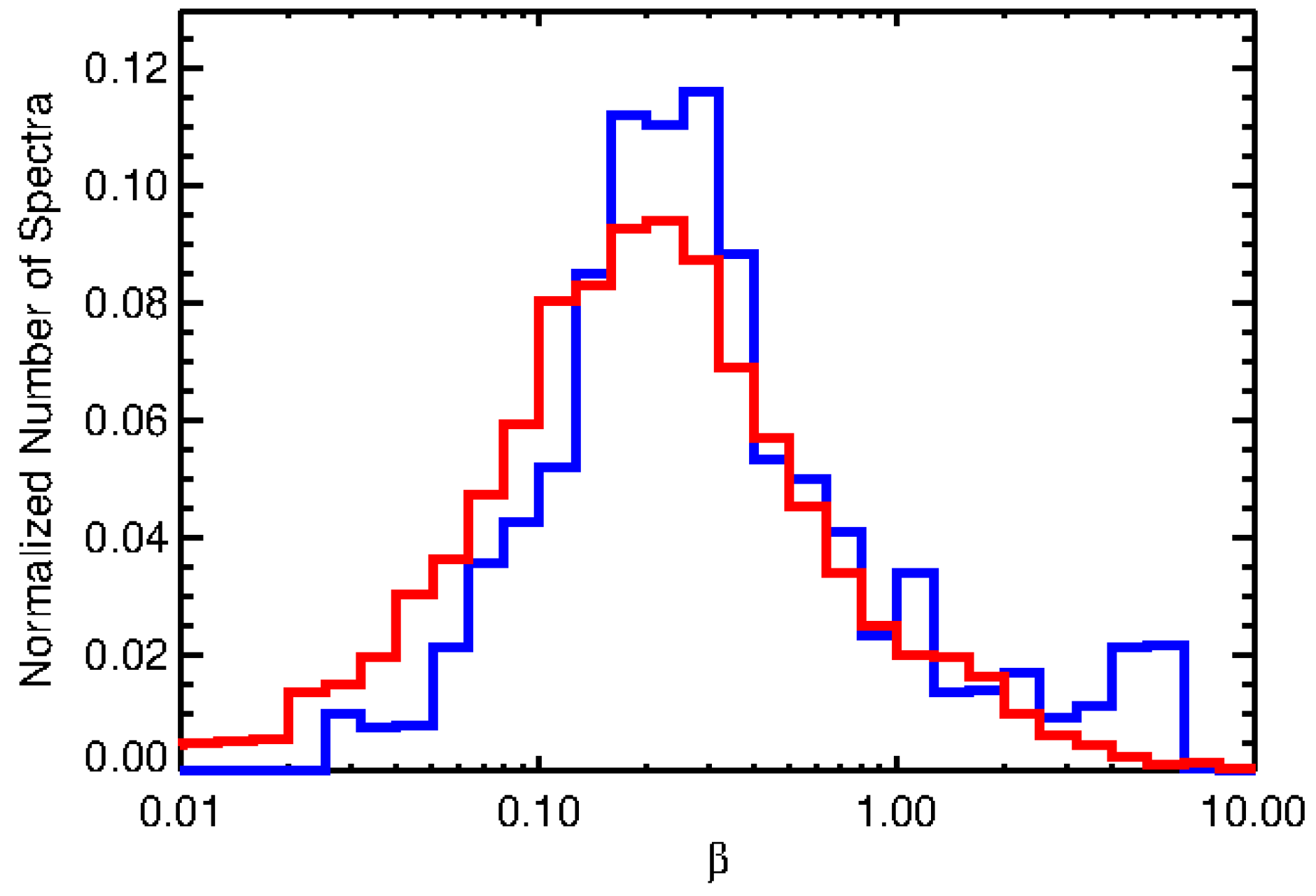
We selected two subsets of our data intervals according to their cone angle ${\mathsf{\Phi }}_{BU}$, that is, the angle between the mean magnetic field and the direction along which the data was collected that corresponds to the solar wind bulk velocity. We chose data intervals with low cone angles, $|{\mathsf{\Phi }}_{BU}-90°| > 60°$, and high cone angles, $|{\mathsf{\Phi }}_{BU}-90°| < 30°$.

The histogram of ion plasma beta for this two groups can be seen in Figure 1. Both distributions are almost superposed, indicating a low correlation between plasma beta and cone angle. For each cone angle group, we selected two new subsets of time intervals, ${\beta }_i\le 0.1$ and ${\beta }_i\ge 0.5$.

The total number of intervals for each category can be found in

Table 1. Number of time intervals gathered according to ion plasma beta, ${\beta }_i$, and mean magnetic field orientation with respect bulk velocity, ${\mathsf{\Phi }}_{BU}$.

	Total	$|{\mathbf{\Phi }}_{\mathbf{BU}}-{90}^{\circ }| > {60}^{\circ }$	$|{\mathbf{\Phi }}_{\mathbf{BU}}-{90}^{\circ }| < {30}^{\circ }$
${\beta }_i\le 0.1$	20,188	760	12,689
${\beta }_i\ge 0.5$	17,904	1566	9512

.

If KAWs play a role into the generation of the transition region in the density spectrum, data intervals with low plasma beta and high cone angles are expected to have a flatter slope at the transition region.

2.2. Simulations Set Up

We use a pseudo-spectral code to solve the 3D compressible Hall-MHD equations with periodic boundary conditions from which we obtain the evolution of density $\rho$, magnetic field $\mathbf{B}$, isotropic pressure P, and velocity fluctuations $\mathbf{u}$.

Length, time, velocity, density, and magnetic field intensity are written in code units as $\mathcal{L}=L_0/\left(2\pi \right)$, $\mathcal{T}=t_{NL}^0=L_0/\left(2\pi u_{rms}^0\right)$, $\mathcal{U}=u_{rms}^0$, $\mathcal{N}={\rho }_{rms}^0$, $\mathcal{B}=B_0/\sqrt{4\pi {\mu }_0}$, respectively. We use ${\rho }_{rms}^0$ to express the initial average density of the plasma, $u_{rms}^0$ is the initial root-mean-square (rms) velocity of the fluctuations, $t_{NL}^0$ is the initial nonlinear time based on the initial rms velocity, and $B_0$ is the background mean magnetic field. The mean magnetic field is aligned with the x direction and the initial amplitude of magnetic fluctuations with respect to the mean field is $|b_{rms}^0|/|B_0|=0.2$, where $b_{rms}^0$ are the initial rms magnetic fluctuations.

The Hall-MHD equations

$$\begin{array}{cc}\hfill D_t\rho & +\rho \nabla ·\mathbf{u}=0\hfill \end{array}$$

(1)

$$\begin{array}{cc}\hfill D_t\mathbf{u}& +\frac{1}{\rho }\left[\nabla (P+\frac{{\mathbf{B}}^2}{2})-\mathbf{B}·\nabla \mathbf{B}\right]=\frac{\mu }{\rho }\left(\Delta \mathbf{u}+\frac{1}{3}\nabla (\nabla ·\mathbf{u})\right)\hfill \end{array}$$

(2)

$$\begin{array}{cc}\hfill D_t\mathbf{B}& -\mathbf{B}·\nabla \mathbf{u}+\mathbf{B}\nabla ·\mathbf{u}=\eta \Delta \mathbf{B}-\nabla \times \left[\frac{\overline{d_i}}{\rho }(\nabla \times \mathbf{B})\times \mathbf{B}\right]\hfill \end{array}$$

(3)

$$\begin{array}{cc}\hfill D_{t}P& +\gamma P\nabla ·\mathbf{u}=\rho \kappa \Delta T+(\gamma -1)\rho Q_{\nu }\hfill \end{array}$$

(4)

$$\begin{array}{cc}\hfill & P=\rho T\hfill \end{array}$$

(5)

are solved in a cubic box of plasma with length $L_0=2\pi \mathcal{L}$ and periodic boundary conditions.

We denote $\overline{d_i}=d_i/\mathcal{L}$ as the proton inertial length normalized by the largest edge of the simulation box, $\gamma =5/3$ and $Q_{\nu }={\mu \left(\right|\omega |}^2+4/3{(\nabla ·\mathbf{u})}^2{)+\eta |\mathbf{J}|}^2$. The heating term $Q_{\nu }$ accounts for the viscuous dissipation of the solenoidal component of velocity fluctuations, ${\mu \left|\omega \right|}^2$, the viscuous dissipation of the compressible component of velocity fluctuations, $\mu 4/3{(\nabla ·\mathbf{u})}^2$, and the resistive dissipation of magnetic fluctuations ${\eta \left|\mathbf{J}\right|}^2$. Here, $\omega =\nabla \times \mathbf{u}$ is the vorticity, $\mathbf{J}=\nabla \times \mathbf{B}$ is the current density and $\mu$, $\eta$, $\kappa$ are respectively the dynamic viscosity, resistivity and thermal conductivity. For all runs $\mu =\eta =\kappa$ in order to simplify the search of optimal values for these three quantities that maximize the (magnetic and kinetic) Reynolds number and allow the energy of the fluctuations to be dissipated before reaching grid-resolution scales.

All numerical simulations are solved with a pseudo-spectral method to compute spatial gradients and a 3rd-order Runge-Kutta scheme for the evolution in time (Wray [36]). The compressible Hall-MHD equations are solved on a three-dimensional uniform grid. All runs have a resolution of 256 grid points in each direction. Velocity and magnetic fluctuations are excited with random phases and are initially purely solenoidal. The two energies are at equipartition at the beginning of the simulations and $b_{rms}^0/\sqrt{{\rho }_{rms}^0}=u_{rms}^0=\mathcal{U}$, where ${\rho }_{rms}^0=1$ in simulation units for all runs. The initial 1D magnetic and kinetic energy spectra are proportional to $k^{-2}$. Velocity and magnetic fluctuations are initially uncorrelated and excited up to a cut-off wave number $k_{max}=4$ for all runs. Conversely, density fluctuations have zero amplitude at the beginning of the simulation.

In simulation units, the sound speed, the Alfvén speed and plasma beta are written as $c_s=\sqrt{\gamma T}$, $v_a=\left|{\mathbf{B}}_0\right|/\sqrt{\rho }$ and $\beta =(2/\gamma ){(c_s/v_a)}^2$. Three different values of plasma beta are used in our simulations, $\beta =0.2$, $0.5$, and 2. We assume the temperature of protons and electrons to be the same in our simulations, $\beta ={\beta }_i+{\beta }_e=2{\beta }_i$. We set values of ${\beta }_i$ within the groups selected for the solar wind data analysis plus one intermediate value. Initial values for $\overline{d_i}$, turbulent Mach number $M^0=u_{rms}^0/c_s$, plasma $\beta$, $\mu$, $\eta$ and $\kappa$ are specified in

Table 2. Initial conditions for all runs in simulation units. $\overline{d_i}=d_i/L_0$ is the proton inertial length normalized by the largest edge of the simulation box; $\beta =(2/\gamma ){(c_s/v_a)}^2$ is the total plasma Beta, where $c_s$ and $v_a$ are the sound speed and the Alfven speed; $M^0=u_{rms}^0/c_s$ is the initial turbulent Mach number; $\mu ,\eta ,\kappa$ column indicates the value of the dynamic viscosity, resistivity and thermal conductivity.

Run	$\overline{{\mathit{d}}_{\mathit{i}}}$	$\mathit{\beta }$	${\mathit{M}}^0$	$\mathit{\mu },\mathit{\eta },\mathit{\kappa }$
Hb02	$0.1$	$0.2$	$0.5$	$1\times {10}^{-3}$
Mb02	0	$0.2$	$0.5$	$1.5\times {10}^{-3}$
Hb05	$0.1$	$0.5$	$0.3$	$1\times {10}^{-3}$
Hb2	$0.1$	$2.$	$0.15$	$1\times {10}^{-3}$

.

2.3. Linear Dispersion Relations in Hall-MHD

We want to verify whether the spectrum of density fluctuations is able to create a flattened density spectrum under plasma conditions similar to those of the solar wind at 1 au. In this context, the $k\omega$ spectrum can serve as a diagnostics for isolating any contribution from wave-like fluctuations (if present). The more energetic wave-like fluctuations in the $k\omega$ spectrum are expected to gather around the dispersion relations predicted from Hall-MHD linear theory, making it possible to classify them according to the their proximity to each dispersion relation. This criteria however, is not sufficient to distinguish between real wave-like and structure-like fluctuations.

The linear dispersion relations for Hall-MHD modes can be computed solving an eigenvalue problem. Firstly, we consider linear perturbations of the form (e.g., for the magnetic field) $\delta B\propto exp\left(i\right(\mathbf{k}·\mathbf{x}-\omega t\left)\right)$. We then apply a Fourier transform to the Hall-MHD equations, leading to $\nabla \to i\mathbf{k}$ and ${\partial }_t\to -i\omega$. The linearized Hall-MHD equations read

$$\begin{array}{cc}\hfill \omega \delta \mathbf{B}& =-\mathbf{k}\times (\delta \mathbf{B}\times {\mathbf{B}}_0)+\frac{\overline{d_i}}{{\rho }_0}(i\mathbf{k}\times \delta \mathbf{B})\times {\mathbf{B}}_0\hfill \end{array}$$

(6)

$$\begin{array}{cc}\hfill \rho \omega \delta \mathbf{u}& =-\mathbf{k}\times (\delta \mathbf{B}\times {\mathbf{B}}_0)+c_s^2\mathbf{k}\delta \rho \hfill \end{array}$$

(7)

$$\begin{array}{cc}\hfill \omega \delta \rho & ={\rho }_0\mathbf{k}·\delta \mathbf{u}\hfill \end{array}$$

(8)

We use the coordinate system defined in Vocks et al. [37], with the $\tilde{x}$ axis aligned with the wave vector $\mathbf{k}$, the $\tilde{z}$ axis being coplanar to $\tilde{x}$ and ${\mathbf{B}}_0$, and $\tilde{y}$ being orthogonal to this plane. Let us also denote the angle between $\tilde{x}$ and ${\mathbf{B}}_0$ as $\mathsf{\Psi }$.

The equations can then be rewritten into the following eigenvalue problem:

$$\mathrm{M}·\mathbf{q}=\frac{\omega }{k}\mathbf{q}$$

(9)

where

$$\mathbf{q}=\frac{1}{v_a}{\left(\frac{c_s\delta \rho }{{\rho }_0},\frac{\delta B_{\tilde{z}}}{\sqrt{{\rho }_0}},\delta u_{\tilde{z}},\delta u_{\tilde{x}},\frac{\delta B_{\tilde{y}}}{\sqrt{{\rho }_0}},u_{\tilde{y}}\right)}^T$$

(10)

and the Hermitian matrix M is:

$$\left(\begin{array}{cccccc}0& 0& 0& c_s& 0& 0\\ 0& 0& -v_{a}cos\left(\mathsf{\Psi }\right)& v_{a}sin\left(\mathsf{\Psi }\right)& ik\overline{d_i}{v}_{a}cos\left(\mathsf{\Psi }\right)& 0\\ 0& -v_{a}cos\left(\mathsf{\Psi }\right)& 0& 0& 0& 0\\ c_s& v_{a}sin\left(\mathsf{\Psi }\right)& 0& 0& 0& 0\\ 0& -ik\overline{d_i}{v}_{a}cos\left(\mathsf{\Psi }\right)& 0& 0& 0& -v_{a}cos\left(\mathsf{\Psi }\right)\\ 0& 0& 0& 0& -v_{a}cos\left(\mathsf{\Psi }\right)& 0\end{array}\right)$$

The eigenvalues of M give the dispersion relation for each linear mode of the Hall-MHD equations: the Alfvén, the slow, and the fast magneto-sonic modes and their respective extensions for wave numbers larger than $k{d}_i=1$, that is, the Kinetic Alfvén Waves (KAW), the Ion-Cyclotron (IC) and Whistler (W) waves.

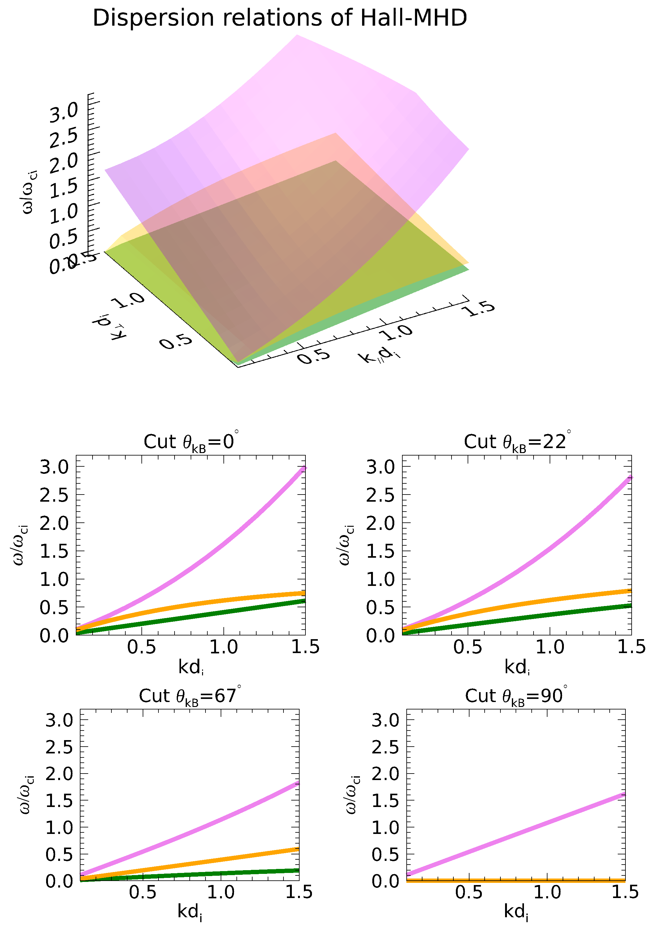
In the top panel of Figure 2 we display the dispersion relations of Alfvén-KAWs (yellow), slow-ICs (green) and fast-Ws (purple) modes in $(k_{\Vert }{d}_i,k_{\perp }{d}_i,\omega /{\omega }_{ci})$ space, taking $\overline{d_i}=0.1$, $\beta =0.2$ and $v_a=5\mathcal{U}$. Here, $k_{\Vert }$ and $k_{\perp }$ stand for the modulus of wave vectors aligned and perpendicular to the mean magnetic field.

2D cuts of the dispersion relation surfaces can be seen below the top panel. Each cut corresponds to the dispersion relations for wave-vectors forming an angle with respect to the mean magnetic field, ${\theta }_{k{B}_0}=0°$, $22°$, $67°$ and $90°$. From Figure 2 we remark that the Alfvén-KAW and slow-IC branches lay at $\omega /{\omega }_i=0$ for ${\theta }_{kB0}=90°$, both are clearly separated from the fast-W branch at any ${\theta }_{kB0}$ and both are almost superposed for quasi-parallel and quasi-perpendicular angles. The importance of these features for the analysis of the $k\omega$ spectrum is discussed in Section 3.2.3.

3. Results

3.1. Data Analysis

Data are divided in intervals of high and low cone angles and high and low plasma $\beta$. For a given subset, we obtain the density spectrum as the median of the spectrum of each interval.

We then fitted the median spectrum to a piecewise function composed of three power laws of the form $f^{-\alpha }$. The ranges of the frequency intervals and the spectral indices were free parameters of the fitting procedure.

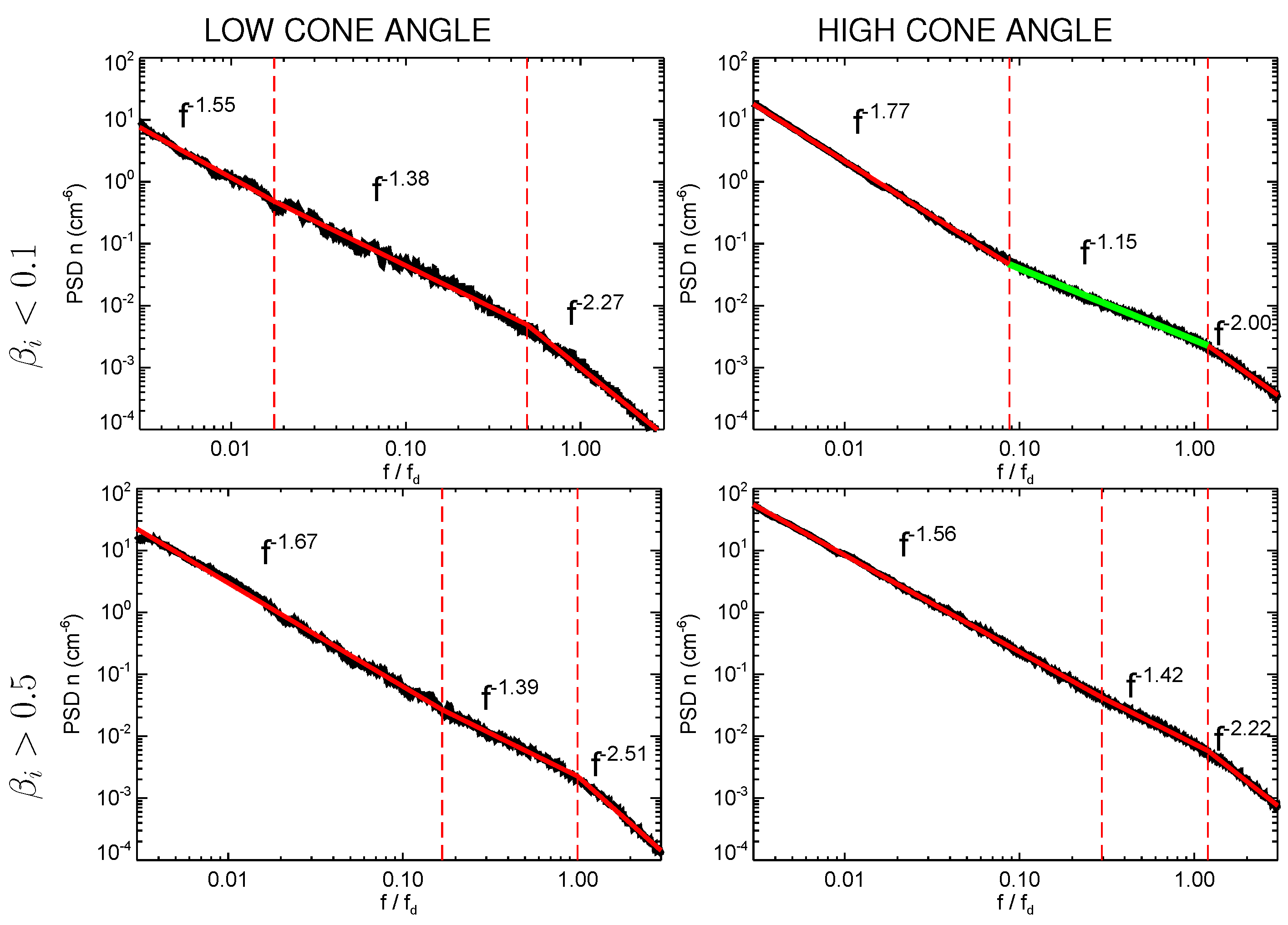
Figure 3 shows the resulting median density spectra computed from data intervals with low and high cone angles (left and right columns) and the selected intervals with plasma ${\beta }_i<0.1$ and ${\beta }_i>0.5$ (top and bottom rows). Frequencies are normalized to $f_d=V_{sw}/\left(2\pi ({\rho }_p+d_i)\right)$ computed over the selected data intervals before taking the median, where ${\rho }_p=V_{th}/{\omega }_{ci}$ is the proton thermal gyroradius, $V_{th}$ the proton thermal velocity, $V_{sw}$ is the solar wind bulk speed in the spacecraft frame and $d_i$ the proton inertial length. The power law intervals are delimited by vertical red dashed lines and the fitted power laws are the red solid lines superposed to the spectra. The fitted power law that displays the region with the more pronounced spectral flattening is in green color in order to highlight it over the rest.

For low beta plasma, high cone angles reveal a clear flattening of the density spectrum, passing from a $f^{-1.77}$ power law to $f^{-1.15}$, with the latter power law being extended over a decade, $[0.10,1.00]f/f_d$. Conversely, for low cone angles, the power law fitting indicates a more subtle flattening, from $f^{-1.55}$ to $f^{-1.38}$. In this case, the transition region extends within the interval $[0.02,0.5]f/f_d$. The mild change in the spectral slope, the wider frequency interval and the fact that it ends half a decade away from $f/f_d=1$ suggests that, for low cone angles, the flattening of the density spectrum could be artificial, consequence of taking the indices and extension of three power laws as fitting parameters.

For low cone angles, density spectrum changes at low frequencies, from $f^{-1.67}$ power law to $f^{-1.39}$, at the interval $[0.20,1.00]f/f_d$. On the other hand, for high-cone angles, the spectrum passes from $f^{-1.56}$ to $f^{-1.42}$ at approximately the same frequency interval.

Unlike for the low beta density spectra, the spectral flattening of density spectra in high beta intervals is comparable for the low and high cone angles data sub-groups. In the high beta density spectra, the flattening is also less abrupt, with spectral indices closer to those fitted at low frequencies.

3.2. Simulation Results

In this section we describe the numerical results obtained from MHD and Hall-MHD simulations initialized with plasma parameters similar to the values measured in the solar wind at 1 AU. We first compute the 1D reduced density spectrum parallel to ${\mathbf{B}}_0$, $E_{\rho }\left(k_x\right)$, and perpendicular to ${\mathbf{B}}_0$, $E_{\rho }\left(k_z\right)$

$$\begin{array}{c}\hfill E_{\rho }\left(k_x\right)=\int \int {|\widehat{\delta \rho }(k_x,k_y,k_z)|}^{2}d{k}_{y}d{k}_z\end{array}$$

(11)

$$\begin{array}{c}\hfill E_{\rho }\left(k_z\right)=\int \int {\left|\widehat{\delta \rho }(k_x,k_y,k_z)\right|}^{2}d{k}_{x}d{k}_y\end{array}$$

(12)

and compare them to observations. In doing so, we will assume the validity of Taylor’s hypothesis e.g., $P_{|{\mathsf{\Phi }}_{BUsw}-90°| >60°}\left(f\right)\approx \frac{2\pi }{U_{sw}}{E}_{\rho }\left(k_x\right)$, and $P_{|{\mathsf{\Phi }}_{BUsw}-90°| <30°}\left(f\right)\approx \frac{2\pi }{U_{sw}}{E}_{\rho }\left(k_z\right)$.

3.2.1. Hall Term Effects on Density Cascade

In order to verify whether the flattened slope in the transition region of the density spectrum is related to Hall term effects, we compare a 3D compressible MHD and a compresible Hall-MHD simulations, Mb02 and Hb02, with initial plasma parameters similar to those encountered in the solar wind when the flattened transition region is observed (${\beta }_i\le 0.1$ and $|{\mathsf{\Phi }}_{BUsw}-90°|<30°$).

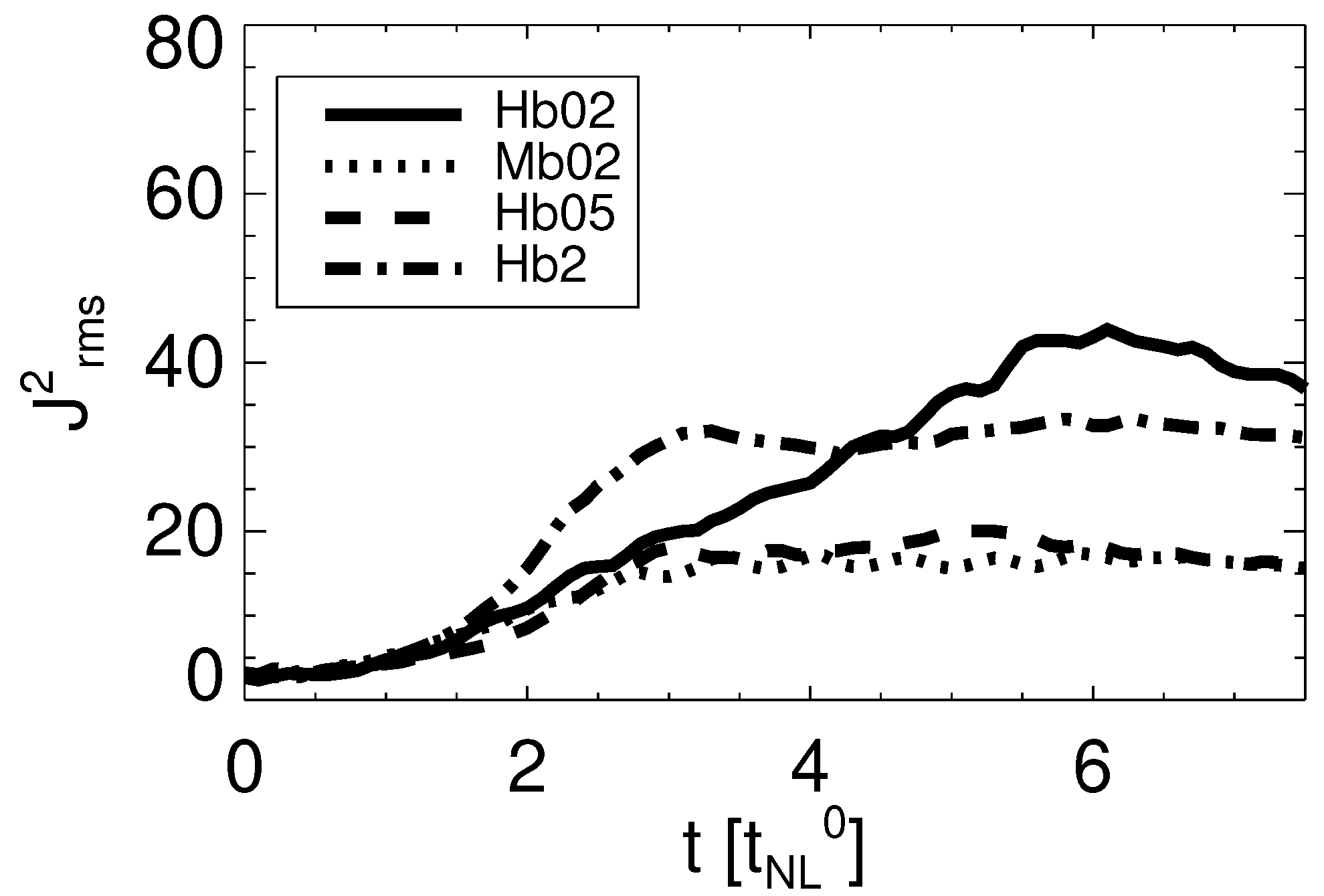
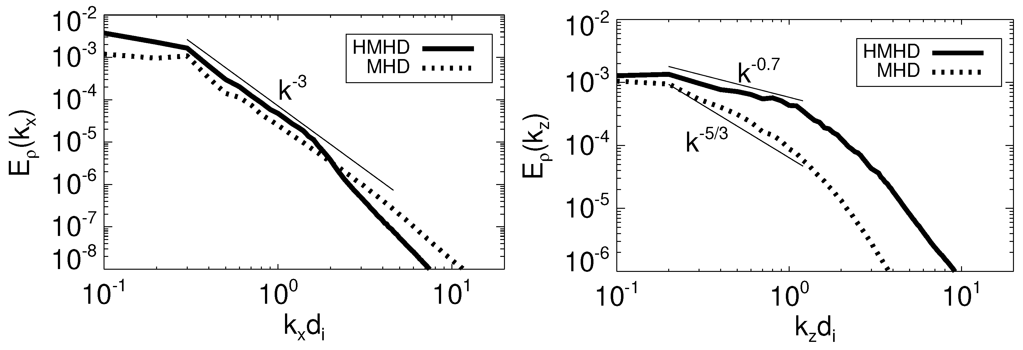
In Figure 4 the time evolution of the current density $J_{rms}^2$ can be seen for all runs. The saturation of $J_{rms}^2$ is reached at $3t_{NL0}$ for runs Mb02, Hb05 and Hb2 and at $6t_{NL0}$ for Hb02. All spectra are averaged over the time interval $[6t_{NL0},7t_{NL0}]$, in which turbulence is fully developed for all runs. In Figure 5, we compare the 1D spectrum of density fluctuations along the x and z axes, parallel and perpendicular directions to the mean magnetic field, for runs Hb02 (solid line) and Mb02 (dotted line).

Both runs have a similar 1D reduced spectrum when measured along the mean magnetic field (left panel of Figure 5) with lower wavenumbers being proportional to $k^{-3}$. Conversely, along the perpendicular direction to ${\mathbf{B}}_0$, for run Mb02 a Kolmogorov’s power law $k^{-5/3}$ is formed, while for run Hb02 the 1D reduced spectrum is proportional to $k^{-0.7}$ (right panel of Figure 5). Note that the differences between MHD and Hall-MHD in the perpendicular direction appear for $k{d}_i<1$. This implies that Hall physics are necessary for the generation of the density spectral flattening.

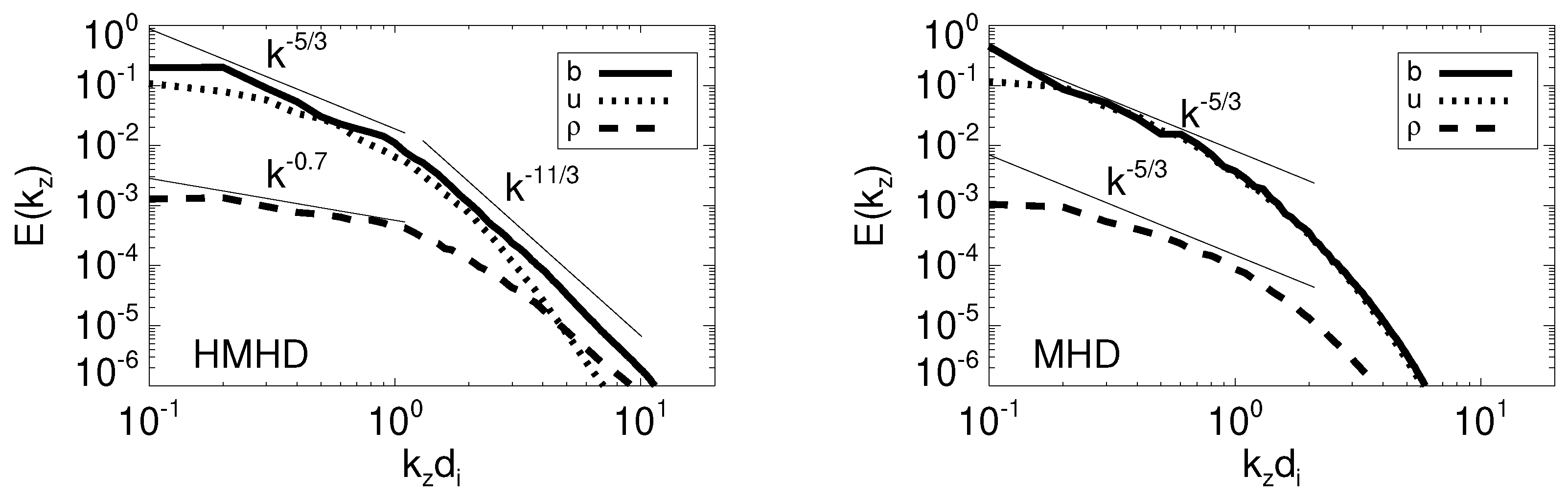
Figure 6 allows to compare the velocity, magnetic and density 1D spectra along the z axis, computed from the temporal average between $6t_{NL0}$ and $7t_{NL0}$ for Mb02 (right panel) and Hb02 (left panel). For the MHD run, Mb02, density acts as a passive scalar, displaying the same $k^{-5/3}$ power law as the velocity and magnetic spectra for run Mb02. Conversely, for the Hall-MHD simulation, Hb02, the velocity and magnetic spectra also follow a $k^{-5/3}$ power law for $k{d}_i\le 1$, but the density spectrum scales as $k^{-0.7}$ in the same range. This difference between the density and the velocity and magnetic spectra when turbulence is fully developed means that density does not behave as a passive scalar in the Hall-MHD simulation.

3.2.2. Is Plasma Beta a Control Parameter?

Despite the limited resolution, the variation of the spectral index with plasma beta found with observations in Section 3.1 is also found in the numerical simulations. In this section we compare the 1D density spectrum for three Hall-MHD simulations, Hb02, Hb05 and Hb2, initialized with plasma beta $\beta =0.2$, $0.5$ and 2 respectively. All of them have the same inertial length $\overline{d_i}=0.1$ and initial mean magnetic field ${\mathbf{B}}_0=(5,0,0)b_{rms}^0$.

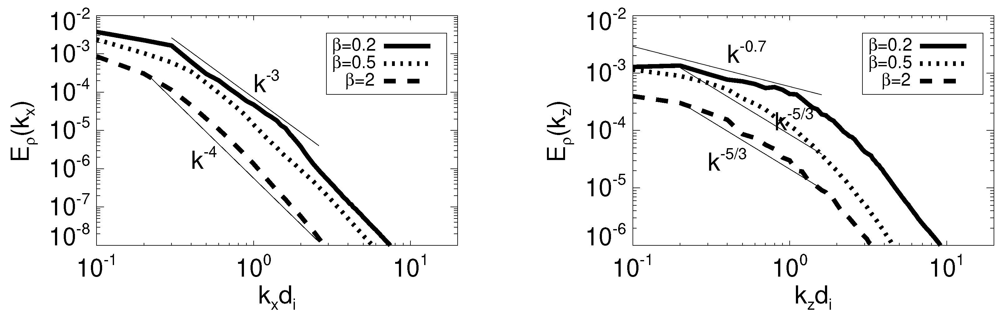
The differences in the reduced spectra of density fluctuations for Hb02, Hb05 and Hb2 averaged between 6 and $7t_{N{L}_0}$ can be seen in Figure 7. The left panel contains the reduced spectra along the x direction, parallel to the mean magnetic field ${\mathbf{B}}_0$. The simulations with $\beta \le 0.5$ have a similar spectral slope at large scales, close to a $k^{-3}$ power law, and is even steeper for $\beta \le 2$, scaling as $k^{-4}$.

The reduced spectra computed along the z axis (perpendicular to ${\mathbf{B}}_0$) are in the right panel of the same figure. In this case, the spectrum steepens for higher beta. While for $\beta =0.2$, the spectrum scales as $k^{-0.7}$ for $k{d}_i\le 1$, for $\beta =0.5$ and $\beta =2$, power laws are closer to $k^{-5/3}$ (consistent with what found in 2D Hall-MHD, Papini et al. [38]). This indicates that high cone angles ${\mathsf{\Phi }}_{BUsw}\sim 90°$ and $\beta \le 0.2$ are necessary conditions to obtain the flat density spectrum (as in observations).

3.2.3. Wave-Mode Decomposition of Density Spectrum

This section is dedicated to the $k\omega$ spectrum of density fluctuations for the only simulation with a flattened density spectrum, run Hb02. We aim to assess whether we can associate the energy of the density fluctuations in the $k\omega$ spectrum with the Hall-MHD linear modes described in Section 2.3.

In order to reduce the computational, cost we did not use the whole 4D $k\omega$ spectrum of density fluctuations, $S_{\rho }(\omega ,k_x,k_y,k_z)=\frac{1}{2}{\left|\widehat{\delta \rho }(\omega ,k_x,k_y,k_z)\right|}^2$. Instead, we use a 3D subset taking $k_y=0$ and denoting it as

$${\tilde{S}}_{\rho }(\omega ,k_x,k_z)\equiv S_{\rho }(\omega ,k_x,0,k_z)$$

(13)

The time interval to produce the $k\omega$ spectrum is the same one used to compute the reduced spectra in Section 3.2, $[6t_{NL0},7t_{NL0}]$. The time-step in the simulations is not constant and depends on the Courant-Friedrichs-Lewy condition. In order to transform the time signal into the frequency spectrum we first linearly interpolated the temporal signal to obtain a constant cadence of $2.5 \times {10}^{-3}{t}_{NL,0}$ or, in terms of the proton gyro-frequency, $0.1{\omega }_{ci}^{-1}$. We then impose periodicity to the temporal signals by applying a window function and computed the Fourier transform for the resulting time signal. The periodization of the time signal creates an artificial spreading of energy for $k{d}_i\le 0.2$ that depends on the applied window function. We chose the Hann window function because it minimized this effect.

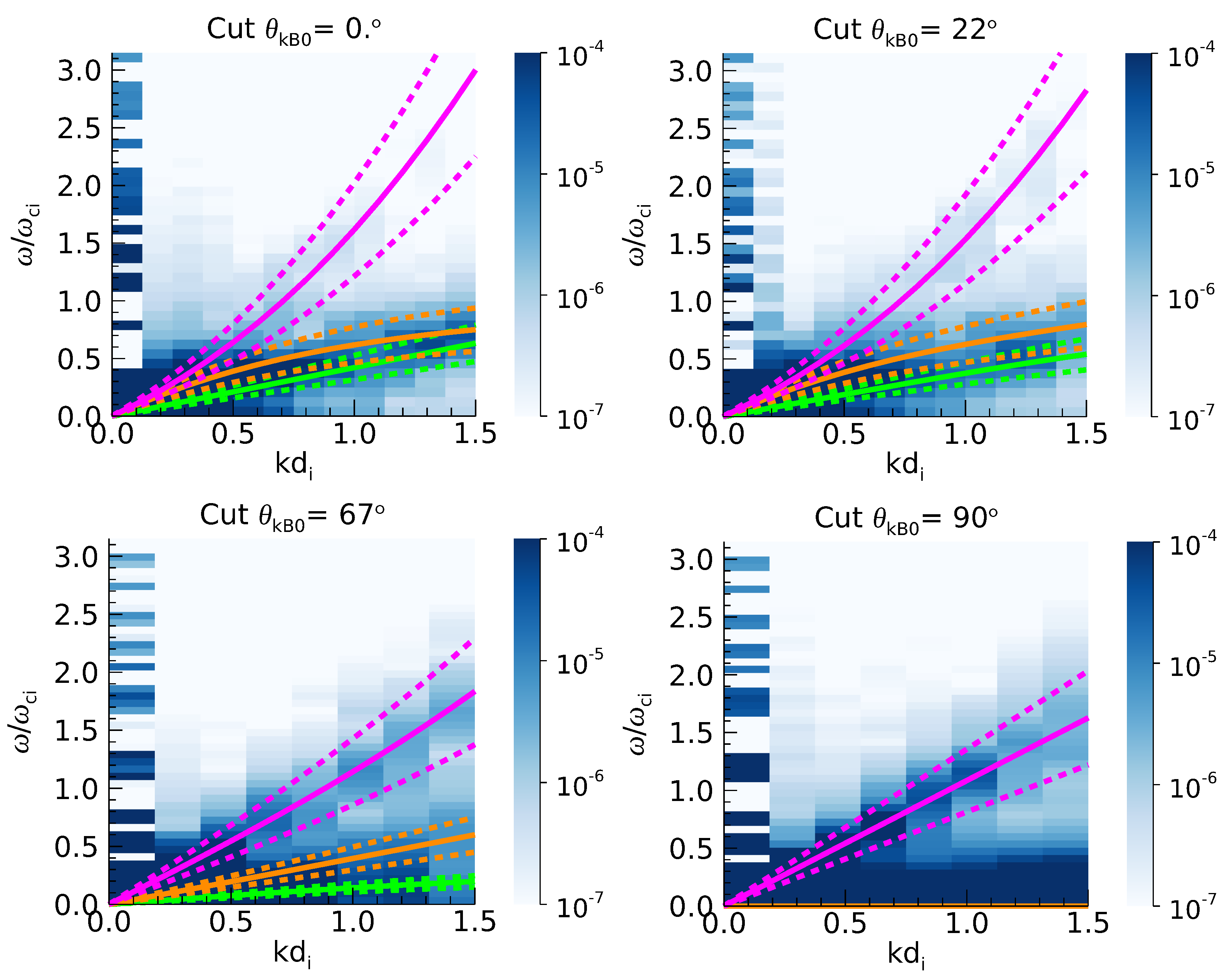
Four 2D cuts of the 3D $k\omega$ spectrum of density fluctuations can be seen in Figure 8. Each cut is taken at angles ${\theta }_{k{B}_0}=0°$, $22°$, $67°$ and $90°$ with respect to the mean magnetic field. The vertical axis corresponds to the normalized time frequencies $\omega /{\omega }_{ci}$ and the horizontal one to the modulus of a wave vector. This selection of angles is arbitrary and only intends to illustrate how the energy of the fluctuations varies with ${\theta }_{kB0}$ in the 3D $k\omega$ spectrum. The blue colorbar indicates the amplitude of the density fluctuations. Solid yellow, purple and green lines correspond respectively to the linear prediction for Alfvén/ Kinetic Alfvén Waves (AW/KAW), the Slow magnetosonic/Ion-Cyclotron (SMS/IC) and fast magnetosonic/Whistler waves (FMS/W), already seen in Figure 2.

Due to the periodization of the time signal, the effect of nonlinear interactions between waves and the spreading of plasma parameters, energy is spread around each dispersion surface. We have taken a tolerance in frequency of $\pm 25\%$ for each dispersion relation in order to delimit the volumes where we expect most of the energy contribution of each mode to be contained. Such tolerance is indicated in Figure 8 with dashed lines around the dispersion relation predictions.

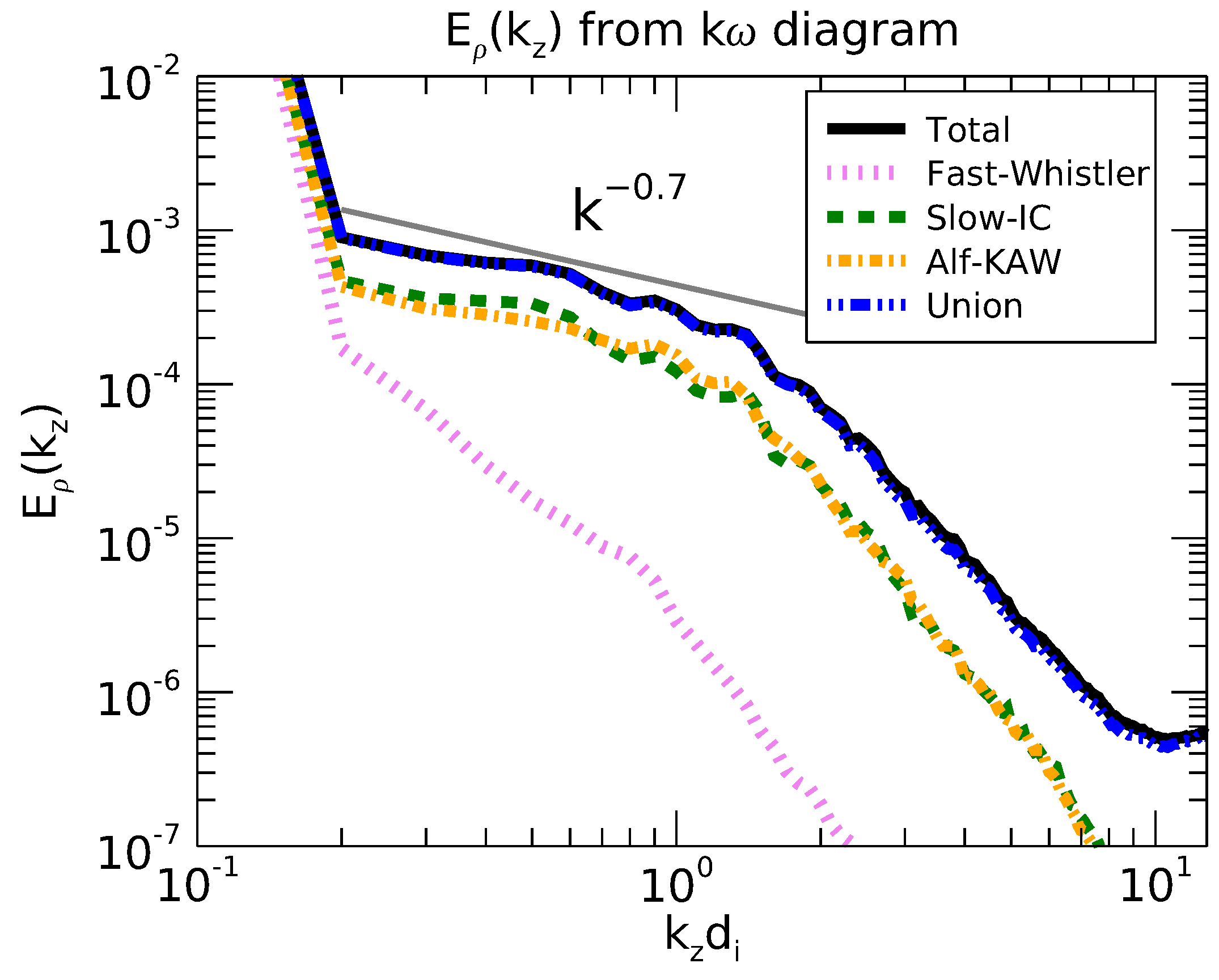
In order to see which mode contributes the most to the flattening, we compute the 1D spectrum of density fluctuations along the $\widehat{z}$ axis from the $k\omega$ density spectrum,

$$E_{total}\left(k_z\right)=\int \int \int S_{\rho }(\omega ,k_x,k_y,k_z)d\omega d{k}_{x}d{k}_y$$

(14)

To obtain $E_{total}\left(k_z\right)$, we compute an approximation of $S_{\rho }(\omega ,k_x,k_y,k_z)$ from the 3D $k\omega$ spectrum by assuming gyrotropy around the mean field axis. Hence, we define the approximated 4D $k\omega$ spectrum as

$$\left\{\begin{array}{cc}\hfill & {\widehat{S}}_{\rho }(\omega ,k_x,k_y,k_z)={\tilde{S}}_{\rho }\left(\omega ,k_x,\sqrt{k_y^2+k_z^2}\right)\mathrm{for}\sqrt{k_y^2+k_z^2}<\frac{\pi N_z}{L_0}\hfill \\ \hfill & {\widehat{S}}_{\rho }(\omega ,k_x,k_y,k_z)=0\mathrm{for}\sqrt{k_y^2+k_z^2}>\frac{\pi N_z}{L_0}\hfill \end{array}\right.$$

(15)

where $N_z$ denotes the spatial resolution along the z direction. The 1D spectrum of density fluctuations, $E_{total}\left(k_z\right)$, computed following the previous procedure is the solid black line in Figure 9. In the same figure, the dotted purple line, the dashed green line and the dotted-dashed yellow line correspond to the contributions associated to the $FMS/W$, $AW/KAW$, and $SMS/IC$ Hall-MHD linear modes. Each contribution has been computed taking the energy of the density fluctuations in volumes surrounding the linear dispersion relation for each Hall-MHD linear mode, $V_{(FMS/W)}$, $V_{(SMS/IC)}$ and $V_{(AW/KAW)}$. The blue line, denoted as Union, corresponds to the spectrum obtained from the integration over the union of all three volumes, $V_{(FMS/W)}\cup V_{(SMS/IC)}\cup V_{(AW/KAW)}$.

All spectra in Figure 9 have a steep decrease from $k_z{d}_i=0.1$ to $k_z{d}_i=0.2$, which is caused by the periodization of the time signal and can be also seen in Figure 8. The Union spectrum is superposed with $E_{total}\left(k_z\right)$, thus implying that most of the energy in the $k\omega$ spectrum lays within the tolerance volumes that we set around each dispersion relation.

Both (AW/KAW) and (SMS/IC) density fluctuations are the main contributors to the sum spectrum. Both of them scales as $k^{-0.7}$. This result could be the consequence of the superposition of volumes $V_{(SMS/IC)}$ and $V_{(AW/KAW)}$ due to the proximity of (AW/KAW) and (SMS/IC) dispersion relations at quasi-parallel and quasi-perpendicular ${\theta }_{kB0}$ angles.

4. Discussion

4.1. Comparison of Observations and Simulations

Observations show a spectral flattening in the spectrum of density fluctuations, with scalings of $k^{-5/3}$ or $k^{-3/2}$ at low frequencies being followed by a power law closer to $k^{-1}$ over one decade above kinetic scales. This flattening increases for low beta plasmas and intervals where the mean magnetic field is quasi-perpendicular to the line along which the data were collected in observations.

With initial conditions similar to the plasma properties used to group the experimental data intervals, 3D Hall-MHD simulations are able to reproduce the flattened region when the reduced density spectrum is measured perpendicularly to the mean field. In particular, for $\beta =0.2$ the reduced density spectrum along the z axis (perpendicular to ${\mathbf{B}}_0$) is proportional to $k^{-0.7}$ over a decade of scales above the inertial range.

In addition, the loss of this transition region when increasing plasma beta is also recovered in simulations. The steepening of the spectrum becomes already clear for $\beta =0.5$ (${\beta }_i=0.25$ with the assumption $T_i=T_e$), that is, one of the most common values for plasma beta in our data intervals. Hence, the flattening of the density spectrum is a feature characteristic of low beta plasmas, ${\beta }_i\le 0.1$.

In the absence of the Hall term, that is, for the standard MHD simulation, the transition region is not formed and the reduced density spectrum perpendicular to ${\mathbf{B}}_0$ have the same $k^{-5/3}$ power law as the magnetic and the velocity spectra. Thus, the effect of the Hall term is necessary to generate the spectral flattening.

Regarding the spectral index anisotropy observed in the experimental data, it also appears in the simulations. However, the density spectra along the mean field are much steeper in the simulations, with spectral indices between $-3$ and $-4$ instead of the $-1.5$ and $-1.8$ from observations. Such effect is common to all runs regardless of the initial plasma parameters. One possible explanation is that the lack of initial energy in the parallel components of the magnetic and velocity fields might prevent the density parallel spectrum from developing a spectral slope closer to observations.

4.2. What Flattens the Density Spectrum?

We attempted to decompose the density spectrum into contributions of Alfvén-KAW, slow magnetosonic-IC and fast magnetosonic-W modes, where this names denote the dispersion relations above and below $d_i$ that are obtained from the linearized Hall-MHD equations.

This analysis reveals that the spectrum can be attributed mainly to density fluctuations below the ion cyclotron frequency. At such frequencies, the energy of the fluctuations accumulates around the Alfvén-KAW modes and slow magnetosonic-IC linear dispersion relations. The spectra generated from integrating the energy surrounding each of these two dispersion relations have the same amplitude and spectral index, $-0.7$.

However, the contributions to the density spectrum associated to Alfvén-KAW and slow magnetosonic-IC dispersion relations are difficult to separate in the $k\omega$ diagram. This is in part due to the artificial spread of energy, consequence of the periodization of the time signal, but also to the spread caused by non-linear interaction of waves, both resulting into the departure of energetic fluctuations from the dispersion relations that linear theory predicts. The spreading and the proximity of Alfvén-KAW modes and slow magnetosonic-IC dispersion relations for quasi-parallel and quasi-perpendicular angles causes that the superposition of contributions associated to both dispersion relations. Finally, it is also necessary to take into account that the energy detected in the Alfvén-KAW and the slow-IC branches may also be associated to slow-evolving structures and not only to wave-like fluctuations.

5. Conclusions

We studied the flattening of the spectrum of density fluctuations at scales above the proton inertial length scale using data from observations at 1 au and 3D compressible MHD and Hall-MHD numerical simulations. The analyzed data intervals were grouped in terms of plasma beta and the cone angle between the mean magnetic field and the direction along which data is collected. This selection shows that the spectral flattening is more pronounced for low plasma beta and high cone angles data intervals.

The numerical results of the Hall-MHD and MHD simulations prove that, under the plasma conditions for which the density spectral flattening is most noticeable in observations, Hall physics is necessary to generate this phenomenon.

Other features of the observations have also been reproduced in the Hall-MHD simulations, such as the steepening of the spectral slope with increasing plasma beta and the spectral index anisotropy of the density spectrum. However the spectral index for the reduced density spectra along the mean field is considerably steeper in simulations.

The $k\omega$ power spectrum of density fluctuations has been computed for the Hall-MHD simulation in which the flattened region of the reduced density spectrum is formed. Via this procedure, we have determined that the main contribution to the spectral flattening corresponds to energetic fluctuations below the ion cyclotron frequency. In particular, the energetic fluctuations surrounding slow magnetosonic-IC (Ion cyclotron) and the Alfvén-KAW dispersion relations are the major contributors to the spectral flattening.

The $k\omega$ diagram is however unable to effectively separate the contribution attributed to slow magnetosonic-IC and the Alfvén-KAW dispersion relations nor to account for the contribution of coherent structures. In future works, we will address this issue by characterizing the polarization properties of the magnetic fluctuations and by using iterative-filtering techniques (Papini et al. [39]).