Article

Experimental Comparative Study between Conventional and Green Parking Lots: Analysis of Subsurface Thermal Behavior under Warm and Dry Summer Conditions

1
Université de Bordeaux, CNRS UMR 5295, I2M Bordeaux, 351 Cours de la Libération, 33400 Talence, France
2
INRAE, LERMaB, Université de Lorraine, 88000 Epinal, France
3
Centre for Ecological Research, Institute of Ecology and Botany, H-2163 Vácrátót, Hungary
4
Department of Climatology and Landscape Ecology, University of Szeged, 2 Egyetem Str., H-6722 Szeged, Hungary
5
Junia, Université de Lille, Université d’Artois, IMT Lille Douai, ULR 4515-LGCgE, Laboratoire de Génie Civil et Géo-Environnement, 59000 Lille, France
6
O2D Environnement, 117 Rue Pierre Brizon, 59810 Lesquin, France
7
Ecole Nationale Supérieure d’Architecture et de Paysage de Bordeaux, Laboratoire GRECCAU, 740 Cours de la Libération, CS 70109, CEDEX, 33405 Talence, France
*
Author to whom correspondence should be addressed.
Atmosphere 2021, 12(8), 994; https://doi.org/10.3390/atmos12080994
Submission received: 7 July 2021 / Revised: 27 July 2021 / Accepted: 29 July 2021 / Published: 31 July 2021

Abstract

:
Green infrastructure has a role to play in climate change adaptation strategies in cities. Alternative urban spaces should be designed considering new requirements in terms of urban microclimate and thermal comfort. Pervious pavements such as green parking lots can contribute to this goal through solar evaporative cooling. However, the cooling benefits of such systems remain under debate during dry and warm periods. The aim of this study was to compare experimentally the thermal behavior of different parking lot types (PLTs) with vegetated urban soil. Four parking lots were instrumented, with temperature probes buried at different depths. Underground temperatures were measured during summer 2019, and the hottest days of the period were analyzed. Results show that the less mineral used in the surface coating, the less it warms up. The temperature difference at the upper layer can reach 10 °C between mineral and non-mineral PLTs. PLTs can be grouped into three types: (i) high surface temperature during daytime and nighttime, important heat transfer toward the sublayers, and low time shift (asphalt system); (ii) high (resp. low) surface temperature during daytime (resp. nighttime), weak heat transfer toward the sublayers, and important time shift (paved stone system); and (iii) low surface temperature during daytime and nighttime, weak heat transfer toward the sublayers, and important time shift (vegetation and substrate system, wood chips system, vegetated urban soil). The results of this study underline that pervious pavements demonstrate thermal benefits under warm and dry summer conditions compared to conventional parking lot solutions. The results also indicate that the hygrothermal properties of urban materials are crucial for urban heat island mitigation.

1. Introduction

The urban heat island (UHI) phenomenon is triggered by several factors, such as the specific urban land cover, the canyon-shaped infrastructure morphology, the anthropogenic heat emissions, and the physical properties of the urban materials [1,2]. Many studies focus on identifying different patterns of urban expansion and their consequences on the urban microclimate [3,4,5,6]. Cai et al. [3] studied the influence of urbanization on the urban climate. They observed that the arrangement of urban areas in relation to water and vegetated areas affects energy fluxes. Several methods are proposed for reporting different types of land use. A major approach is the use of land cover indices [7,8], followed by the classification methods [9]. Jalan and Sharma [10] used land surface temperature (LST) to quantify the spatiotemporal changes in the UHI of Jaipur city (India). They found that urbanization affects the LST by about 3 °C.
Urbanization processes tend to increase the fraction of sealed and impervious surfaces. However, urban facets significantly influence the urban climate. Urban facets often demonstrate specific hygrothermal properties (e.g., low albedo, and reduced water absorption and retention), which lead to extreme surface temperature.
The development of sustainable and resilient cities requires alternative solutions and concepts, such as nature-based solutions (NBS) or green infrastructure (GI) [11]. Zölch et al. [12] reported that GI affects pedestrians’ thermal comfort. They conducted a study on high-density residential areas under current and future climatic conditions. GI (planting trees) demonstrates the strongest impact with an average physiological equivalent temperature (PET) reduction of 13% compared with existing vegetation. At ground level, several new pavement technologies are emerging, including pavement watering, reflective pavement, pervious pavement, and heat storage pavement [13].
Green parking lots (GPLs) are now being suggested as potential solutions for urban water management and UHI mitigation [14]. Onishi et al. [14] studied the influence of vegetation on urban parking in Nagoya city, Japan, during the warm period (spring and summer). They showed that parking with grass slightly reduced the LST (maximum LST decreased by 7.26 °C in the summer for one GPL). Park et al. [15] conducted a study of GPLs in Ulsan, Korea. They observed that the replacement of pavement materials reduces the radiant temperature of the surface. Considering the anthropogenic nature of its soil layers, a GPL can be considered as an urban soil or Technosol [16]. Pervious GPL systems included porous layers that retain water. Evaporation of stored water contributes to a cooling down perception for pedestrians and a sensible reduction of air ambient temperature [17]. In addition, GPLs could reduce surface temperature if vegetation is included [18].
Several studies show the importance of vegetation and biobased materials (e.g., wood chips) on the GPL behavior [19]. Wood chips may be locally produced and originate from sustainably managed forest. In addition, Buchanan et al. [20] argued that wood chips can be a solution adapted to the urban context because of their effectiveness in controlling soil erosion on a steeply sloping construction site.
Wang et al. [21] presented two types of driving factors for the evaporative cooling performance of pervious materials, namely the climatic parameters [22] and the hygrothermal parameters (albedo, water absorption, and water retention properties) [23]. Solar radiation has been reported to be the most significant climatic parameter, followed by air temperature, relative humidity, and wind speed [22].
Hygrothermal properties of pervious pavement are usually assessed under controlled conditions [24]. However, performance observed during laboratory experimental tests must be consolidated with summertime case studies of pervious pavement implemented at full scale. During dry and warm periods, water availability within pervious pavements may shrink dramatically. In these conditions, evaporation may be strongly reduced, and the cooling benefits of GPLs may be weakened. In the case of pervious concrete, Nemirovsky et al. [25] suggest that water stored far from the surface does not participate in the evaporation process.
Previous studies have shown that, without precipitation, pervious pavements may increase the urban overheating due to their high specific heat capacity and reduced evaporation [26]. Therefore, thermal performance of full-scale GPLs needs to be analyzed to investigate the extent to which pervious pavements can be considered as heat sinks during warm and dry periods. This study aimed to analyze experimentally the thermal behavior of four full-scale parking lot systems under dry and warm summer conditions. To highlight the thermal dynamics and the heat transfer patterns between the different layers, heat and cooling rates were calculated.
This analysis is organized as follows. Section 2 illustrates the study area, data, and methods. It also presents the design of the studied GPL. Section 3 analyzes and discusses the characteristics of the GPLs in terms of thermal performances.

2. Materials and Methods
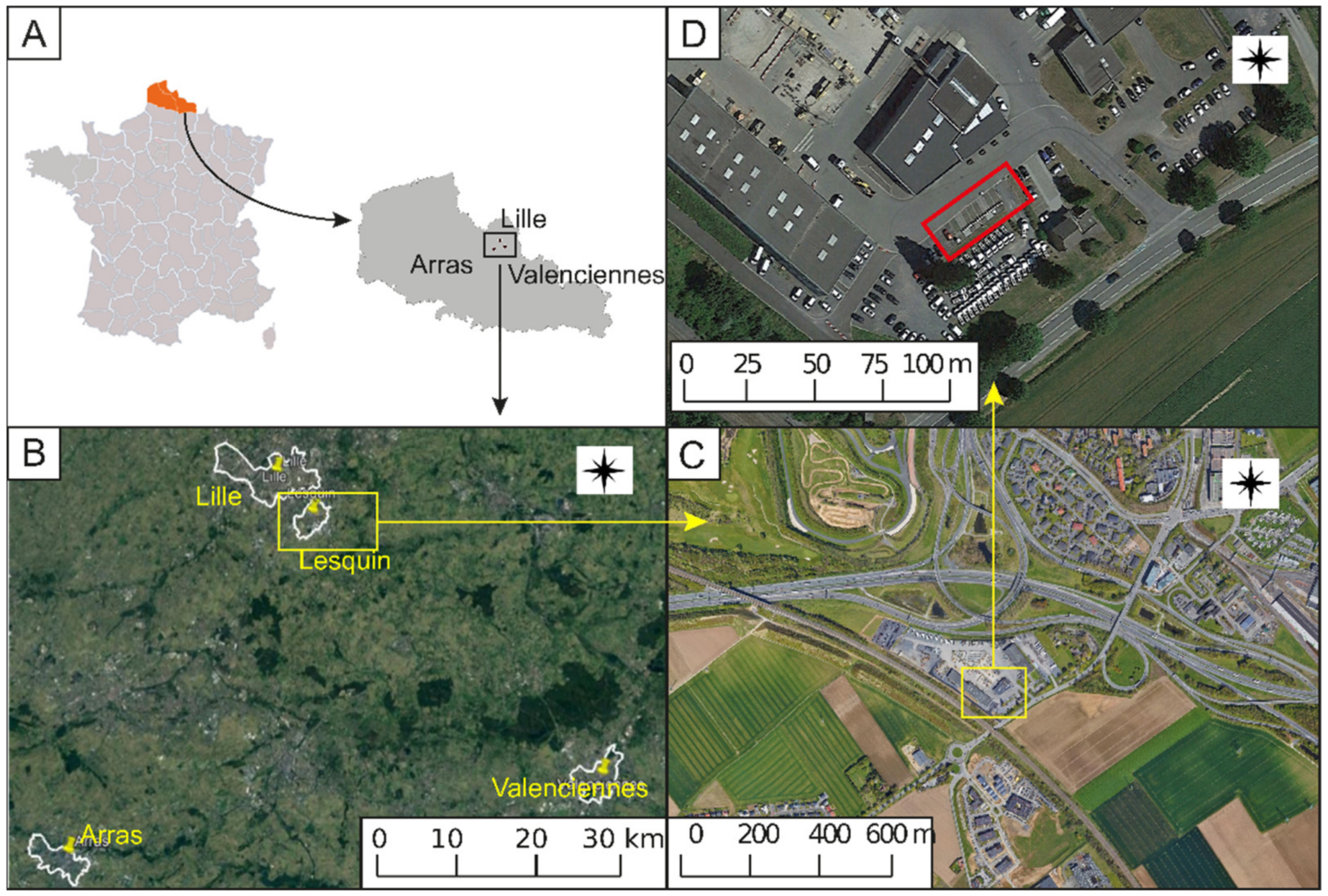
2.1. Study Site

This study was conducted in northern France within the conurbation of Lille (Figure 1A). It is the sixth largest French conurbation and has 1,100,000 inhabitants. Located approximately 50 km south of the North Sea, Lille experiences a temperate oceanic climate (Cfb climate in the Köppen Geiger classification system [27]). July is the warmest month of the year, with an average maximal (resp. minimal) air temperature of 23.3 °C (resp. 13.8 °C) [28]. July is also the wettest month of the summer, with 68.5 mm of precipitation on average. The mean month insolation values for June, July, and August are, respectively, 206, 211, and 199 h [28].
To date, the urban climate of Lille has been little investigated; therefore, data to estimate the amplitude of Lille’s UHI are scarce. However, under a calm and clear sky, several values of the UHI amplitude are available for nearby cities with a similar background climate: 4.4 °C for Nancy, France (conurbation population: 286,000 inhabitants) [29]; a maximum of 6 °C for Ghent, Belgium (conurbation population: 560,000 inhabitants) [30]; and up to 8 °C for Paris, France (conurbation population: 10,800,000 inhabitants) [31]. According to these results and to the conurbation size, the UHI amplitude of Lille could be estimated to be between 4 and 7 °C under a calm and clear sky.
The studied parking lots are situated in the city of Lesquin (50°34′56.35″ N 3°07′8.40″ E), in the southern part of the conurbation (Figure 1B). At the local scale, the experimental site belongs to a small industrial settlement, which was built between a highway and agricultural fields (Figure 1C,D).

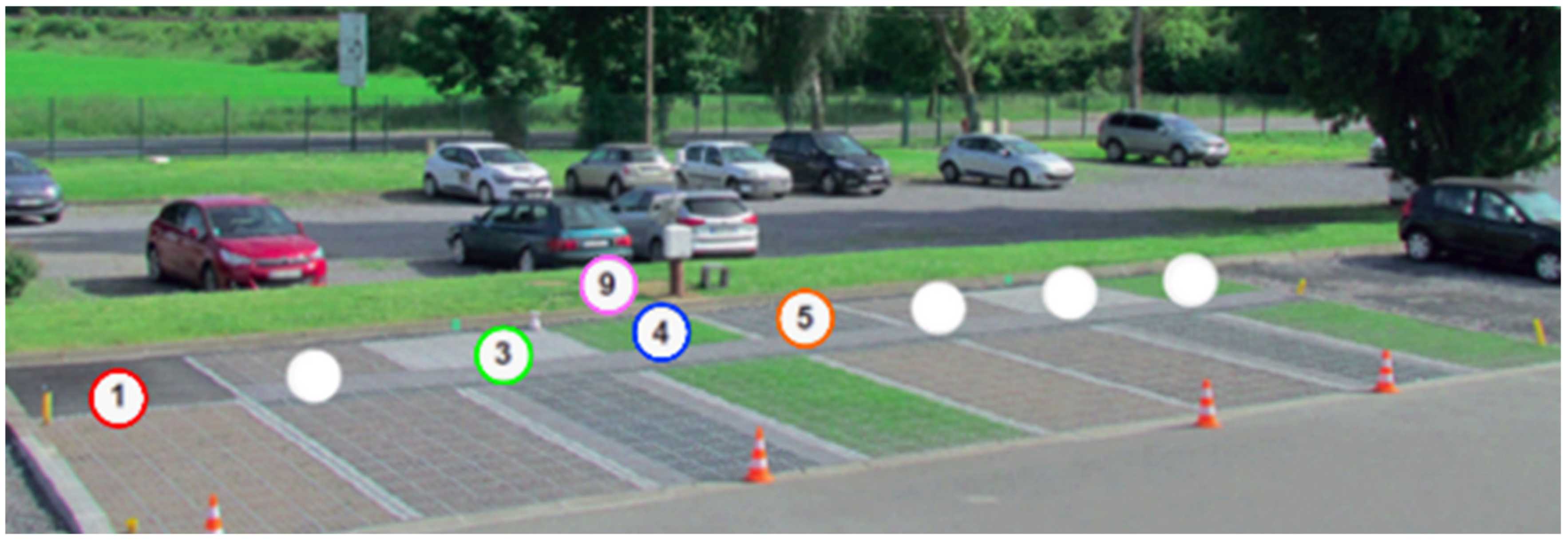
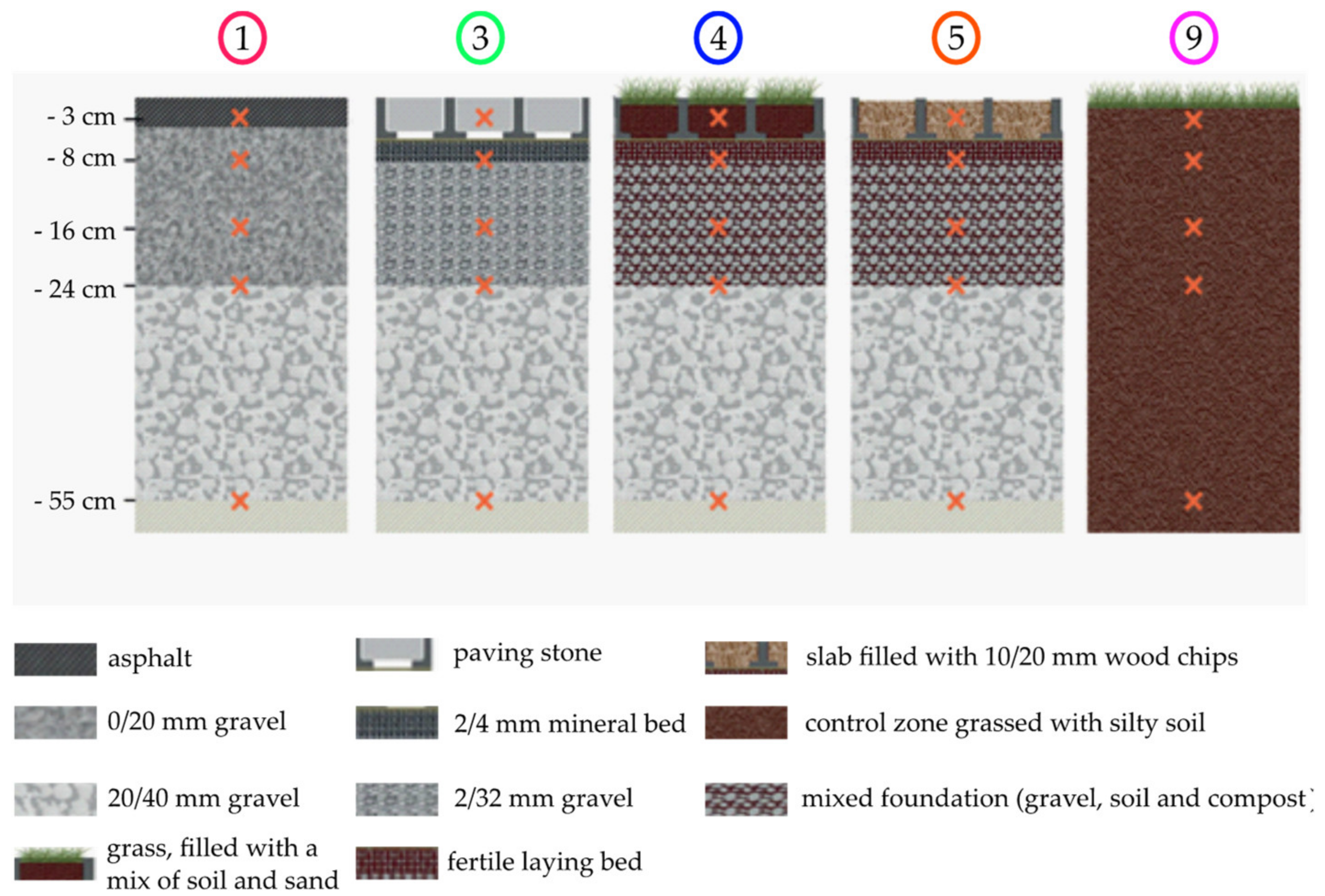
2.2. Structure and Composition of Studied Parking Lots

Eight parking places were built on the Experimental Platform (EP) of Lesquin by construction companies (Figure 2). Due to technical issues, data are available for only four parking lots. The composition of the parking lots is presented in Figure 3 and in Table 1.
The control zone CZ9 is defined as a grass-covered area with silty soil (thickness 55 cm). The four parking lot systems (P1, P3, P4, and P5) are laid on a subfoundation of 20/40 mm gravel (thickness 20 cm). Their composition and structure are described from upper layer to deeper layer:
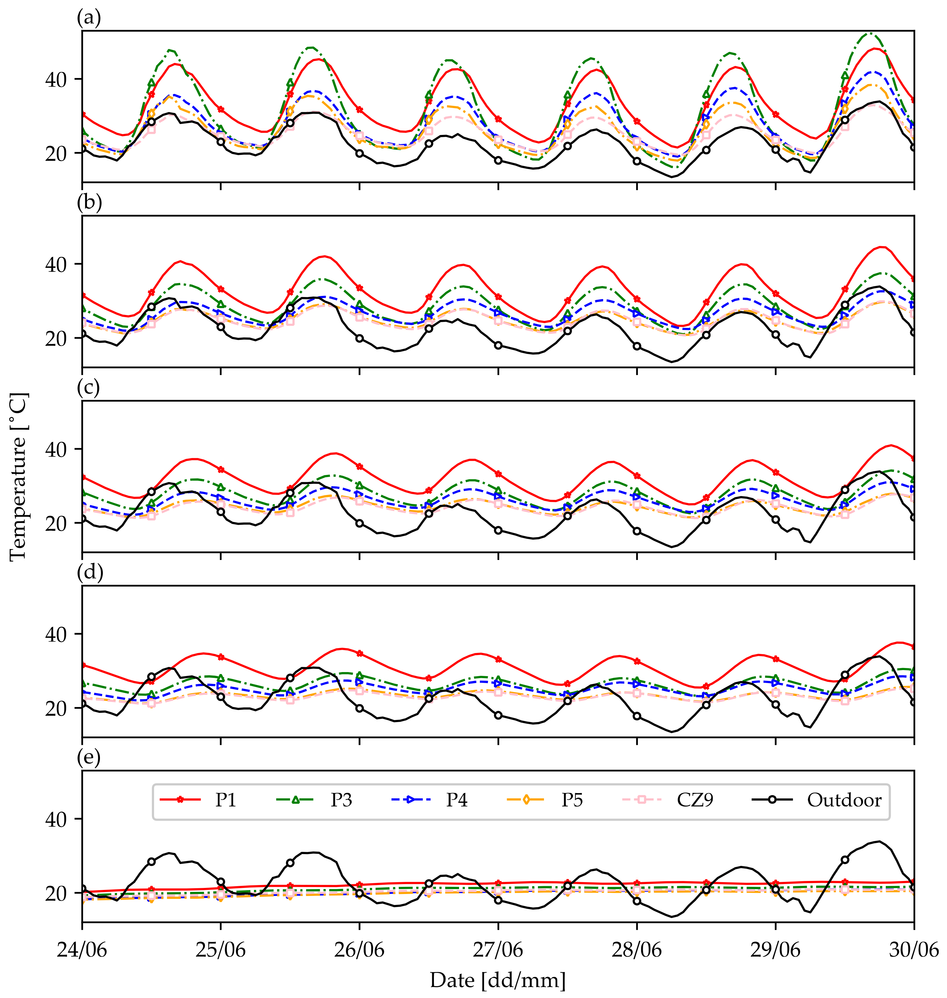
  • The parking lot P1 is a conventional system composed of asphalt (thickness 5 cm) with a 0/20 mm gravel foundation (thickness 15 cm).
  • The parking lot P3 is composed of a slab filled with concrete paving stones (thickness 6 cm), a 2/4 mm mineral bed (thickness 3 cm), and a 2/32 mm gravel foundation (thickness 15 cm).
  • P4 is built up of a grass-covered slab filled with a mix of soil and sand (90% soil and compost, 10% sand 0/4 mm, thickness 6 cm), a fertile laying bed (60% sand, 20% sand 0/4 mm, and 20% soil and compost 0/10 mm, thickness 3 cm) and a mixed foundation (75% gravel, 25% soil and compost, thickness 15 cm).
  • P5 is composed of a slab filled with 10/20 mm wood chips (forest mulch, thickness 5 cm), a fertile laying bed (70% sand, 30% soil and compost, thickness 3 cm), and a mixed foundation (75% gravel, 25% soil and compost, thickness 15 cm).
The slab is a plastic structure made of recycled polypropylene and polyethylene, which provides the required mechanical properties for parking lot use (Figure 4). It represents approximately 39% of the total surface of the parking lot.
Table 1 summarizes the information of the four PLs and CZ9, and Table 2 and Table 3 present the physical properties of the studied materials.

2.3. Materials

Probes were placed during the construction phase of the four parking lots. Different depths were chosen to analyze different construction materials (filling, bedding, foundation, and subfoundation).
Five probes were installed in each of the four parking lots and in an adjacent grassed area (control zone, CZ9). Two types of thermal probes were used: Campbell Scientific CS107 (temperature accuracy of ±0.4 °C) probes were buried at depths of −3, −8, −24, and −55 cm; and Campbell Scientific CS255 (temperature accuracy of ±0.4 °C) probes were buried at −16 cm (Figure 3 and Figure 4). The probes were located in the center of the parking lot, assuming that this center point was not affected by other adjacent parking lots. The width of the parking lot was 2.4 m. The distance between the center of a given parking lot and an adjacent parking lot was 1.2 m.
Table 2 summarizes the physical properties of the constituent materials of the four GPLs and the CZ9.
Outdoor temperature and relative humidity probes (Campbell Scientific CS215) and a rain gauge (Campbell Scientific Kalyx-RG, Loughborough, UK) were also installed. These sensors were connected to a data logger (Campbell Scientific CR1000× Series) powered by a battery connected to a solar panel (Campbell Scientific SP30) (Figure 5). Temperature values were recorded with a 5-min time step between 1 June 2019 and 31 August 2019.

2.4. Key Performance Indicators of Parking Lot Dynamics

To evaluate the dynamics of the parking lots, several key performance indicators were used. Hourly variation of underground temperature between 1 June 2019 and 31 August 2019 was analyzed. The temperature difference with respect to the control zone (CZ9) was calculated (Equation (1)). The ΔT experimental error was ±0.8 °C based on the temperature measurement:
Δ T = T j   c m P i T j   c m C Z
where Tj cm is the temperature (°C) at each depth j = −3, −8, −16, −24, −55 cm, for each parking lot Pi = 1, 3, 4, 5.
The rate of change (RC) was considered to investigate the thermal behavior of the parking lots over time, because this approach has been adopted in previous urban climate studies [41,42,43,44]. The analysis was based on the sixty-minute average temperature to calculate the hourly RC (°C h−1) (Equations (2) and (3)):
R C = T m e a n t
where Tmean (°C) is the average temperature during the previous 60 min and t is time (hour). Tmean was used to calculate RC. The RC experimental error was ±0.4 °C h−1 based on the temperature measurement.
The standard deviation function was also used. This expresses the dispersion of a dataset relative to its mean [45]:
S d = x i μ 2 N
where Sd is the population standard deviation, N is the size of the population, xi is the value from the population, μ is the population mean.

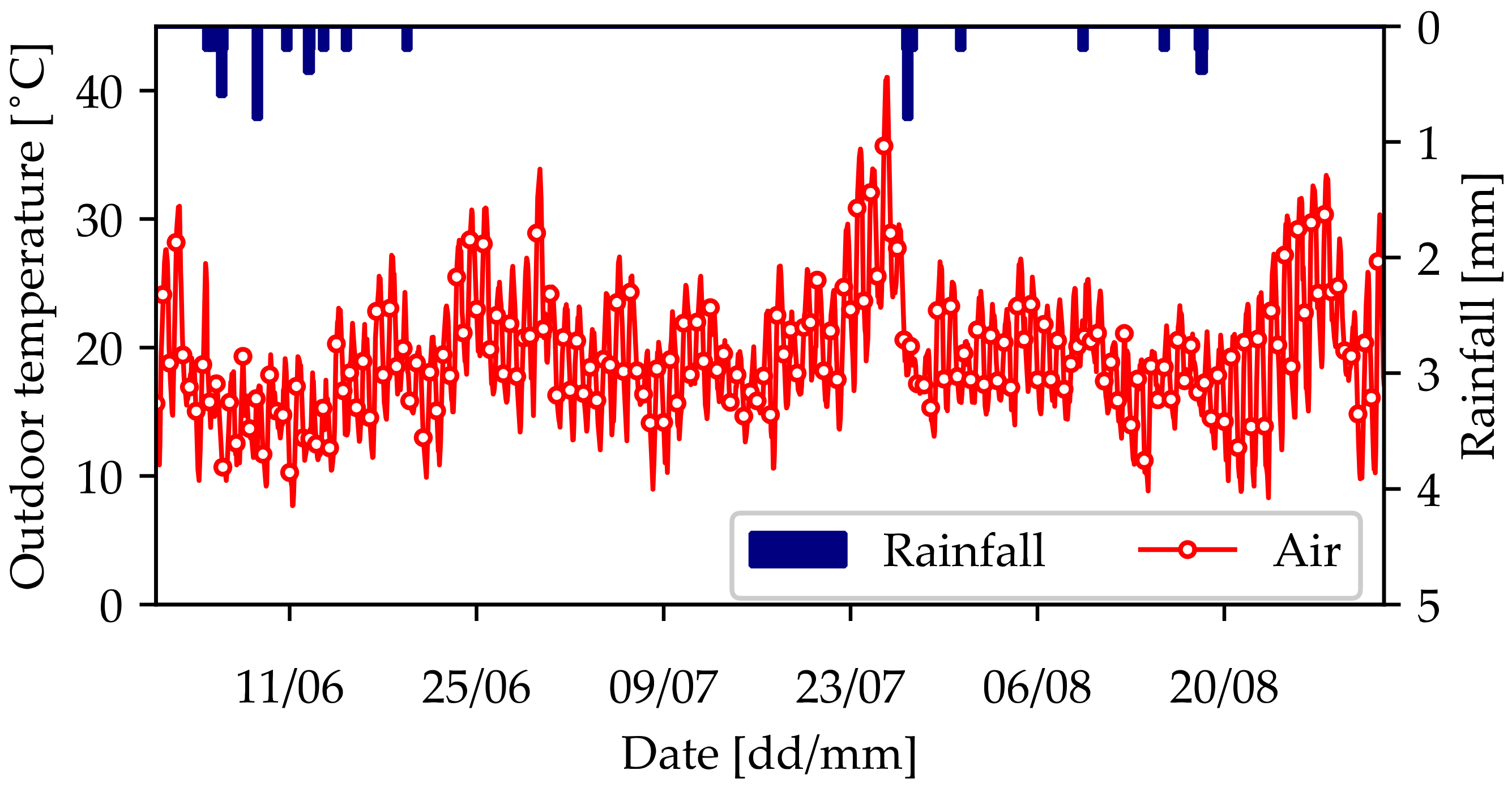
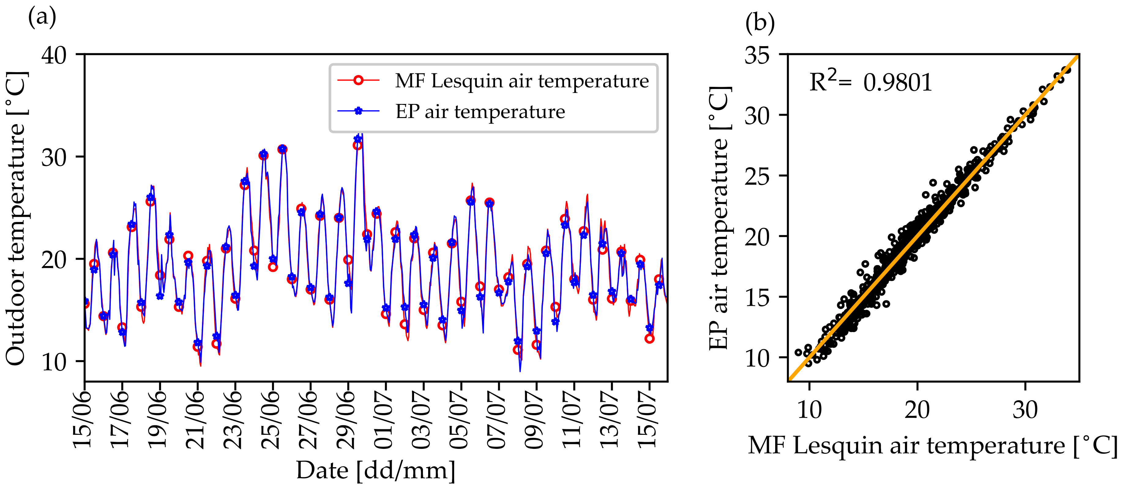
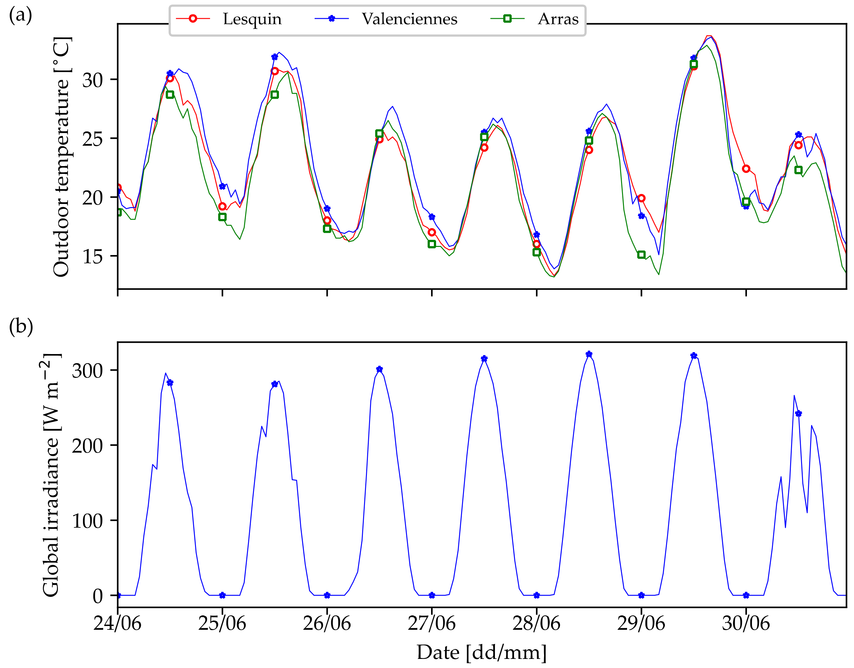
2.5. Local Air Temperature and Rainfall Observations

Data (outdoor temperature and rainfall quantity) from the weather station were obtained over a 3-month period from June to August 2019 (Figure 6). During this period, the outdoor temperature was particularly high and set new records [46,47]. The air temperature varied from 7.7 to 41.0 °C, with an average value of 19.2 °C, and a total rainfall of 7.4 mm. The end of June 2019 demonstrated very warm weather. The outdoor temperature reached 35.2 °C on 29 June. This period (24 June–1 July 2019) was selected to evaluate the thermal behavior of the GPLs during very warm weather. RC was analyzed during the warmest period of summer 2019 (25–26 June 2019).
Figure 7 compares the air temperature measurements from the Experimental Platform (EP) presented in Figure 5 with the nearby weather station operated by Météo France (MF), located at Lesquin Airport. The Lesquin MF weather station is part of the national weather observation network, and is located 4 km from the EP. It appears that the EP air temperature and the air temperature from the MF weather station of Lesquin were similar during the analysis period (Sd-MF Lesquin = 4.53 °C and Sd-EP = 4.41 °C) (Figure 7a). Figure 7b shows that the correlation between the two temperature datasets was strong (R2 = 0.98). Therefore, the difference in the weather between the EP and Lesquin airport can be considered as negligible. A small amount of precipitation was recorded between 15 June and 19 June (14.9 mm). From 20 June to 5 July, no rain was observed.
To gather climatic information regarding the period of interest, the weather observation datasets of Arras and Valenciennes were analyzed. These two cities are located 42 and 38 km, respectively, from the EP (Figure 1).
Figure 8 presents weather variables for three Météo France weather stations in Lesquin, Valenciennes, and Arras during the study period (24 June to 30 June 2019). During this period, global irradiance (experimental error of ±7 W.m−2) increased to 300 W m−2, except for 30 June (cloudy day), when the radiation was less than 250 W m−2 and recorded drops to between 100 and 130 W m−2 (Figure 8b). Air temperatures were very similar (1–2 °C difference) between the three cities (Figure 8a). Based on this similarity in terms of outdoor temperature, it can be hypothesized that the global downward solar radiation is similar at the Météo France weather station of Valenciennes and the Experimental Platform of Lesquin.
The frequency distribution of wind speed and wind direction between 24 June 2019 and 30 June 2019 are presented in Figure 9 for different Météo France weather stations: Lesquin (a)–(b), Valenciennes (c)–(d), and Arras (e)–(f). The prevailing wind is North-East for the three cities. The mean wind speeds are between 4 and 4.5 m s−1 for all locations. The most frequent wind speed is 4.5 m s−1 for Lesquin (frequency 11.2%), 4.5 m s−1 for Valenciennes (frequency 10.5%), and 4.8 m s−1 for Arras (frequency 13.0%). As in the case of the temperature, the wind profiles of these three weather stations were very close.

3. Results

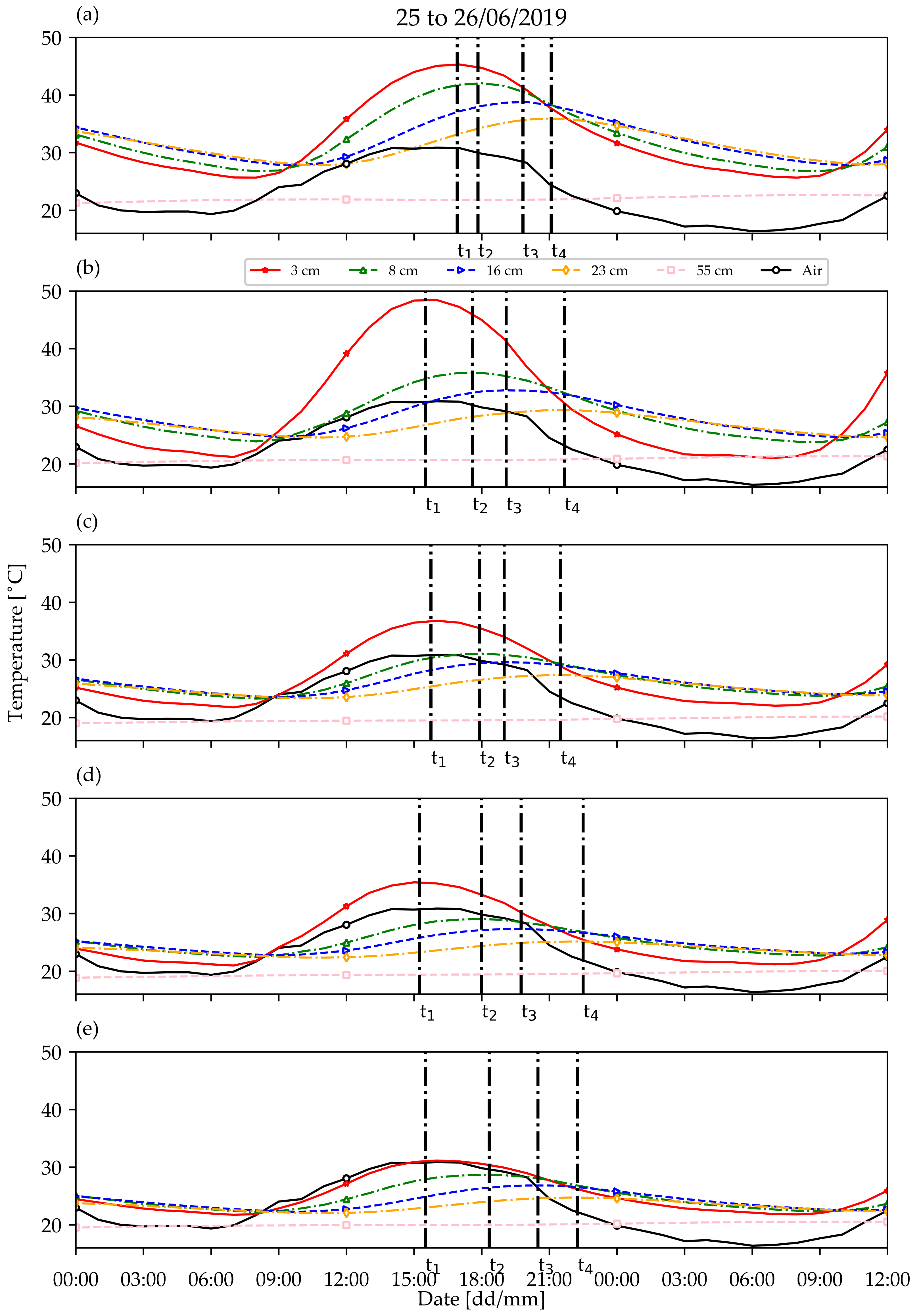
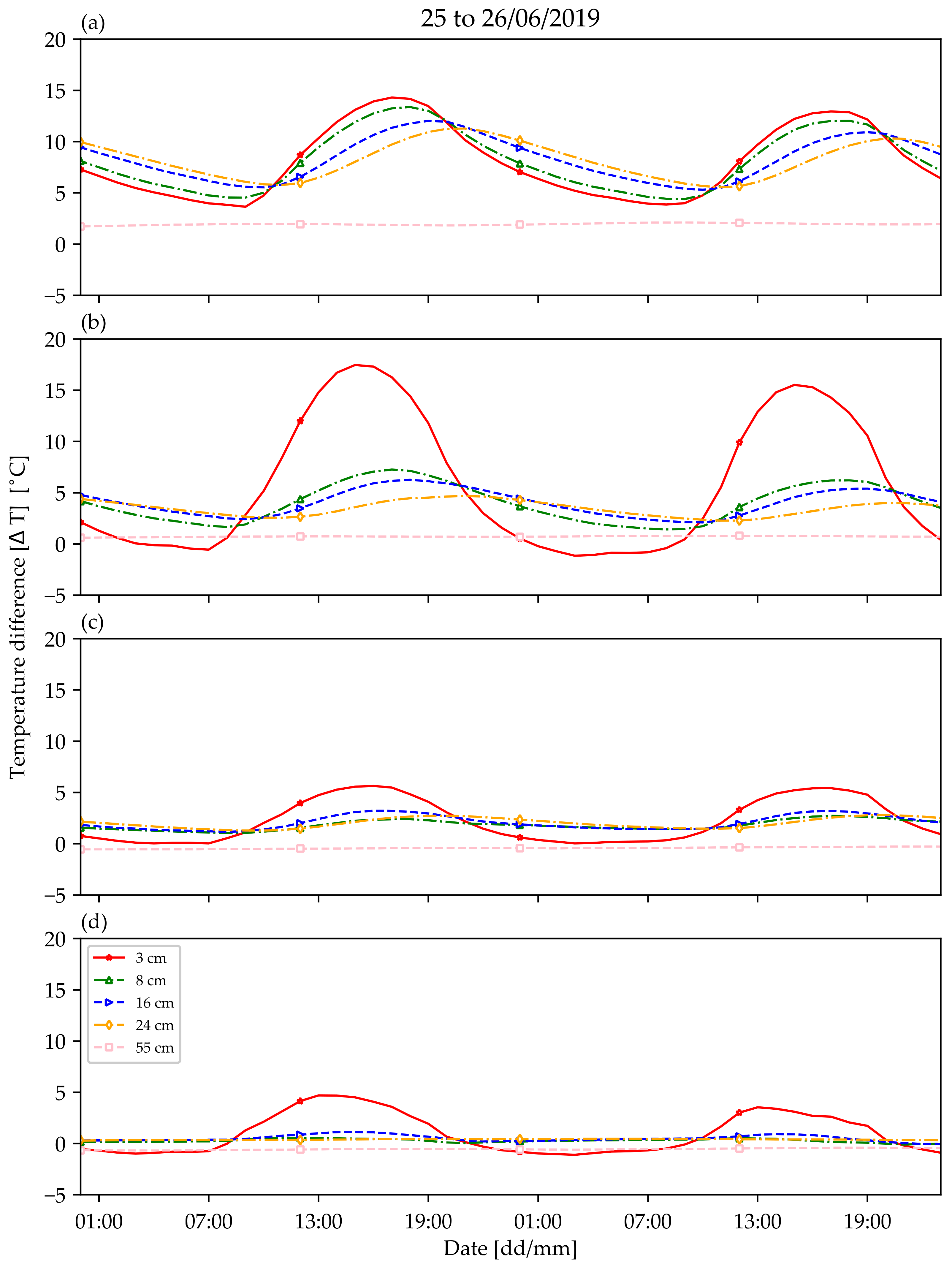
3.1. Impact of Depth on Temperature Dynamics

Temporal variations of temperature of the parking lots (P1, P3, P4, and P5) and control zone (CZ9) at −3, −8, −16, −24, and −55 cm depths between 24 June and 30 June are shown in Figure 10. In general, the daily amplitude of temperature variations tended to decrease with increasing depth. The outdoor air temperature varied between 13.4 and 33.8 °C during this period. Temperatures at −3 cm were higher than the outdoor air temperature for all parking systems.
For the depth of −3 cm (Figure 10a), P3 was the warmest area during daytime and reached a maximum temperature of 51.0 °C. This confirms the existence of an energy storage effect, which induces an increase in the temperature. P3 also exhibited the highest daily temperature amplitude.
At a depth of −3 cm, P1 was the second warmest area during daytime and the warmest area during nighttime. For this depth, P1 was the warmest parking lot on average during the week (33.1 °C).
The temperature fluctuations of P4 (vegetation and substrate) recorded at a depth of −3 cm demonstrated a similar pattern to that of P5 (wood chips) on the first day. A difference in temperature between P4 and P5 began to occur on the third day (3–4 °C at noon). This small temperature gap may be explained by the hydrophilic properties of wood chips (considered to be an organic mulching) because wood may capture part of the morning dew.
CZ9 with grass and natural soil was the coolest area during most parts of the day. The lowest surface temperatures were recorded for CZ9 (29.6 to 32.9 °C at noon).
The depths of −8, −16, and −24 cm demonstrated similar patterns (Figure 10b–d). P1 was the warmest area at all times (day and night). P3 and P4 were cooler than P1, and P5 and CZ9 were the coolest areas. P3 tended to be warmer than P4 during daytime, but the two lots exhibited similar minimum temperatures. P5 and CZ9 showed almost identical thermal behavior. Each PLT presented a repeatable daily temperature pattern.
Measurements at a depth of 55 cm indicated similar patterns and described a plateau (between 18.2 and 22.7 °C). The amplitudes of the variations and the temporal shift, which were particularly visible on the temperature peaks, were negligible (Figure 10e).

3.2. Analysis of the Daily Temperature Cycle

The daily vertical heat transfer cycles were analyzed by the temperature profiles measured at different depths (Figure 11). For all systems, the depth of −3 cm demonstrated the highest temperature amplitude. The temperature amplitude decreased when the depth increased. During daytime, the heat received on the surface was transferred downward by conduction to the lower layers (−8, −16, and −24 cm depths). A daily maximum temperature was observed for all layers, except for the depth of −55 cm. However, the maximum temperature time differed between layers and time shifts were observed. The deeper the layer, the later the daily maximum temperature occurred.
At the beginning of the evening, the −3 cm depth layer started to cool due to convection and radiative transfer. During all the evenings and nights, the lower layers released the stored heat, and the conduction transfer was oriented upward.
The outdoor temperature was much lower than the layer temperatures of P1 and P3 (Figure 11). In the cases of P4 and P5, the temperature at −3 cm (resp. at −8, −16, and −24 cm depths) was higher than (resp. similar to) the outdoor temperature. It appears that CZ9 exhibited a temperature at −3 cm that was comparable to or slightly higher than the outdoor temperature (Figure 10).
Considering P1, the daytime conductive heat transfer toward the lower layers was fast and effective. The time shifts observed for P1 between the daily maximum temperatures (−3, −8, −16, and −24 cm depths) were the lowest of all the studied systems. Moreover, the P1 system stored solar energy in the superficial layer (second warmest daytime temperature at −3 cm depth) and efficiently transferred the heat toward the sublayers (warmest daytime temperature at −8, −16, and −24 cm depths).
P3, P4, and P5 systems included a slab at the superficial layer (between 0 and −6 cm depths). Results indicate that this element played a minor role regarding the thermal behavior of PLT, because the P3 system showed a significantly different underground temperature than that of the P4 and P5 systems.

3.3. Comparison between Studied Systems and Control Zone

Figure 12 presents the temperature differences between each parking lot (P1, P3, P4, and P5) and the control area (CZ9) (cf. Equation (1)). In the case of P1 (Figure 12a), from a depth of −3 to −24 cm, an increase in depth led to a decrease in the daily amplitude and a time shift in the daily temperature extrema. At −55 cm depth, the difference between P1 and CZ9 was almost negligible (0 to 2.0 °C).
The P3 system remained cooler than P1 on average (Figure 12b) for all depths except that of −3 cm. The paved stone was up to 19.5 °C warmer than the control zone during daytime but was cooler than grass during nighttime (−3.5 °C). The paving stone layer (P3) stored a significant amount of heat and increased its temperature. However, it transferred less heat toward the lower layers than P1.
P4 and P5 systems were consistently cooler than P1 (0 to 5.0 °C) (Figure 12c,d). During nighttime, the temperature at a depth of −3 cm was similar to that of CZ9. The difference in temperature reached approximately +9.0 °C for P4 and +5.0 °C for P5 during daytime. P4 demonstrated a positive difference in temperature for −8, −16, and −24 cm depths (average of 2.3 °C), and no temperature gap for the −55 cm depth. Except for the −3 cm depth, the temperature differences between P5 and CZ9 were not significant.

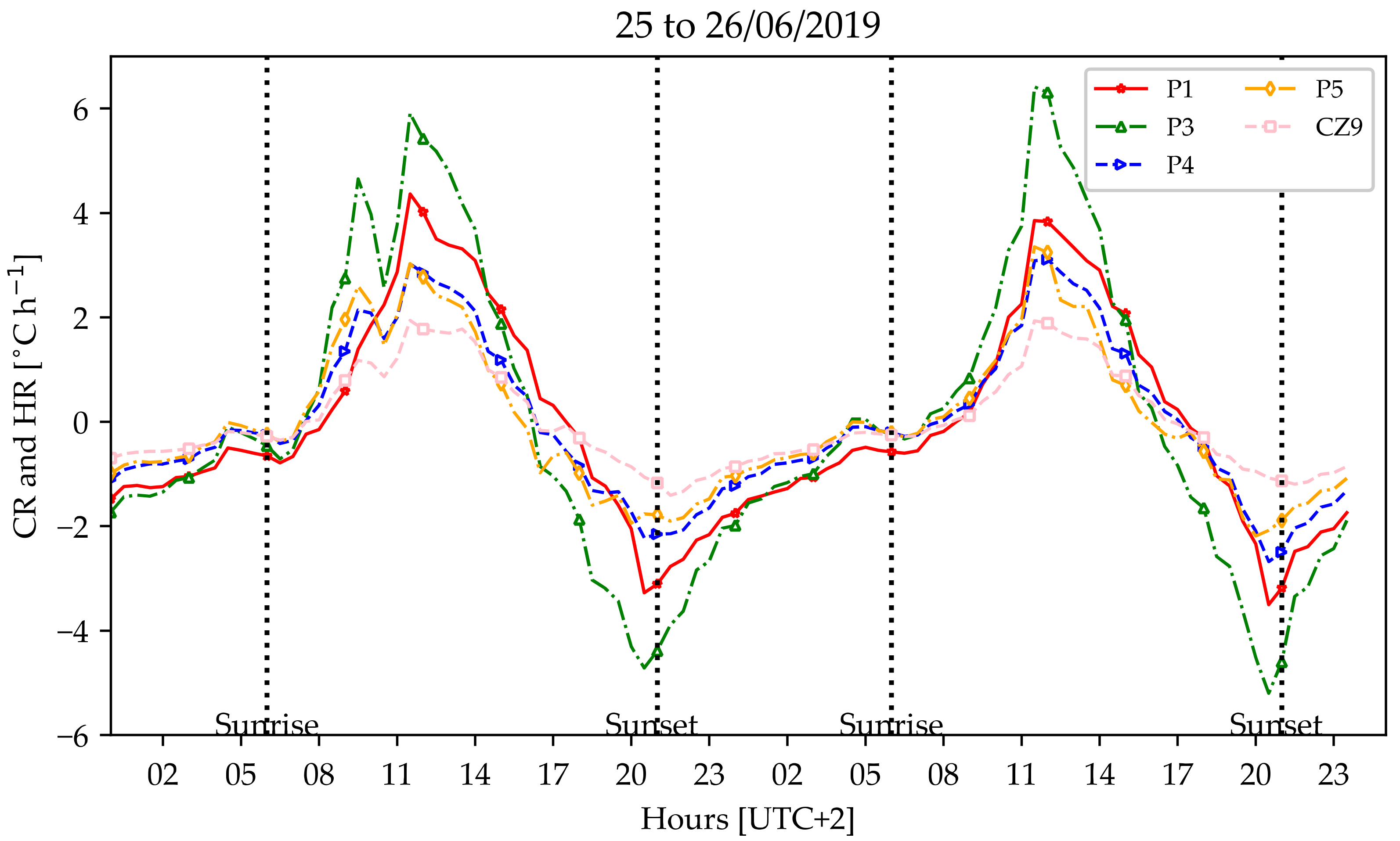
3.4. Cooling and Heating Rates

The cooling and heating rates were calculated for the −3 cm depth on 25 June and 26 June 2019 (cf. Equations (2) and (3)) (Figure 13). Two hours before and after sunrise, all RC rates tended to be similar (between 0.0 and 1.0 °C h−1). Heating started 1–2 h after sunrise (positive value of temperature rate, i.e., heating rate). The heating rates increased and reached their daily maximum around noon. The −3 cm depth layers started to cool around 5 pm (negative value of temperature rate, i.e., cooling rate). The daily minimum in the cooling rate was reached around sunset.
Results illustrate that P3 had the highest RC (corresponded to the heating phase during daytime (up to 6.0 °C h−1 at noon, UTC + 2) and the lowest RC during nighttime (−5.0 °C h−1). P1 demonstrated less intense temperature rates than P3 (maximum RC 4.0 °C h−1, minimum RC −3.0 °C h−1). The P4 and P5 systems had very similar thermal behavior during both day and night. The RC of P4 was, on average, 0.2 °C h−1 higher than the temperature rate of P5. CZ9 showed the smallest amplitude of RC (+2.0 °C h−1 during daytime, −1.5 °C h−1 during nighttime).

4. Discussion

As stated by Hendel et al. [37], the surface material acts as a solar energy receiver and the underground material acts as a form of energy storage. In this study, several solar energy receivers were investigated. The high surface temperature reached by the asphalt cover (P1) is in line with the work of Ca et al. [48], who studied the impact of asphalt paved parking lots in Tokyo, Japan, during the warm period (August to September 1994). Results highlight that the surface temperature at noon rose to 55 °C. Therefore, the solution with asphalt causes an increase in the adjacent air temperature through sensible heat release [49].
The results show the capacity of the paving stone to store a remarkable amount of heat during daytime, and to release it rapidly during the evening and night [50]. Qin and Hiller [51] conducted an experimental study on the pavement-surface energy balance in the Mediterranean climate of dry, hot summers in Davis, California, USA. In this study, most of the absorbed solar energy was transferred into the material via thermal conduction.
The grass cover of P4 and CZ9 appears to be beneficial to the thermal behavior. The presence of vegetation may attenuate the daily amplitude of the temperature [52,53].
Foundations play a role in thermal storage. From a depth of 24 to 55 cm, the foundations of P1, P3, P4, and P5 systems were mineral. As a result, the heat transfer from the surface to the underlying layers was reduced due to the low energy storage capacity of the gravel [51,54,55].
This experimental study suggests that improvements can be undertaken on several PLTs. A modification of the paving stone color (P3) and slab color (P3, P4, and P5) would impact their albedo and may reduce the peak daytime temperature. For instance, Wang and Akbari [56] showed that higher albedo paving can reduce the UHI effect during the day.

5. Conclusions

This study investigated the reaction of pervious pavement, such as green parking lots, in terms of thermal behavior during warm and dry weather conditions. It compared the thermal behavior of different parking lot types (PLTs): a conventional asphalt parking lot (P1), a grass-covered natural soil (CZ9), and three alternative parking lot systems (concrete paving stone (P3), grass-covered slab filled with a mix of soil and sand (P4), and slab filled with wood chips (P5); the latter lots are considered as green parking lots (GPLs)). Results underline that the less mineral the surface coating, the less it warms up. The temperature difference at the upper layer can reach 10 °C between mineral and non-mineral PLTs.
It was found that P1 is the least appropriate modality in an urban heat island context: it heats up quickly, reaches very high temperatures, and transmits heat to the deeper layers of soil. P3 is an intermediate solution. It heats up very quickly and reaches high temperatures that warm the boundary layer. It also cools very quickly and does not store heat over several days. The two solutions that provide results closest to the thermal behavior of natural soils are the P4 and P5 solutions. The lawn became partially dried during this study, which clearly reduced the action of vegetation on soil temperature.
This study highlights that the parking lots systems can be grouped into three types: (i) high surface temperature during daytime, moderate temperature during nighttime, important heat transfer toward the sublayers, and low time shift (P1); (ii) high surface temperature during daytime, low temperature during nighttime, weak heat transfer toward the sublayers, and important time shift (P3); and (iii) low surface temperature during daytime, low temperature during nighttime, weak heat transfer toward the sublayers, and important time shift (vegetation and substrate P4, wood chips P5, control zone CZ9). This highlights that pervious pavements demonstrate thermal benefits during warm and dry periods compared to conventional parking lot solutions. In these weather conditions, GPLs including vegetation or wood chips can obtain thermal performances close to those of grass-covered areas with silty soil.
Results provide insights into how alternative parking lots can affect atmospheric and underground urban heat islands. Because the size of parking lots may range from hundreds to thousands of square meters, urban materials and innovative parking lot solutions need to be assessed in real conditions before being installed at a larger scale. Moreover, the thermal behavior of PLTs should be investigated under warm and dry weather conditions, which are likely to be frequently observed in the coming decades. The output of this research can be valuable for modelling purposes, which is also an important field of climate-smart urban decision making. Subsurface heat transfer for nontraditional solutions must be better understood and modelled. The experimental results presented in this study are worthy to be integrated into numerical modelling approaches.

Author Contributions

Conceptualization, F.L., C.P. and S.D.; Data curation, R.B., F.L., M.P. (Margaux Pierret) and J.B.; Formal analysis, R.B., F.L., M.P. (Margaux Pierret), C.P., S.D., B.L., Z.A. and T.V.W.; Funding acquisition, F.L., C.P., S.D., B.L. and J.B.; Investigation, F.L., M.P. (Margaux Pierret), C.P., S.D., B.L. and J.B.; Methodology, F.L., M.P. (Margaux Pierret), C.P., S.D. and B.L.; Project administration, F.L., C.P., S.D., B.L. and J.B.; Resources, M.K., M.P. (Margaux Pierret), T.V.W., R.G., B.C., A.P., P.L. and M.P. (Mathieu Pétrissans); Supervision, F.L. and J.B.; Validation, F.L., Z.A., T.V.W., R.G. and B.C.; Visualization, R.B.; Writing—original draft, R.B. and F.L.; Writing—review & editing, R.B., F.L., M.K., C.P., S.D., B.L., J.B., Z.A., T.V.W., R.G. and B.C. All authors have read and agreed to the published version of the manuscript.

Funding

This research was funded by ADEME under the initiative IPME 2016 Eau & Milieux Aquatiques, grant number 1782C0085.

Institutional Review Board Statement

Not applicable.

Informed Consent Statement

Not applicable.

Data Availability Statement

Not applicable.

Acknowledgments

All the authors would like to thank the anonymous reviewers for their comments and suggestions, which helped to improve the quality of the manuscript.

Conflicts of Interest

The authors have submitted a declaration of competing interests to the editors.

References

  1. Danh, L.T.; Truong, P.; Mammucari, R.; Foster, N. A Critical Review of the Arsenic Uptake Mechanisms and Phytoremediation Potential of Pteris Vittata. Int. J. Phytoremed. 2014, 16, 429–453. [Google Scholar] [CrossRef]
  2. Di Sabatino, S.; Barbano, F.; Brattich, E.; Pulvirenti, B. The Multiple-Scale Nature of Urban Heat Island and Its Footprint on Air Quality in Real Urban Environment. Atmosphere 2020, 11, 1186. [Google Scholar] [CrossRef]
  3. Cai, D.; Fraedrich, K.; Guan, Y.; Guo, S.; Zhang, C.; Zhu, X. Urbanization and Climate Change: Insights from Eco-Hydrological Diagnostics. Sci. Total Environ. 2019, 647, 29–36. [Google Scholar] [CrossRef]
  4. Cai, Y.; Zhang, H.; Zheng, P.; Pan, W. Quantifying the Impact of Land Use/Land Cover Changes on the Urban Heat Island: A Case Study of the Natural Wetlands Distribution Area of Fuzhou City, China. Wetlands 2016, 36, 285–298. [Google Scholar] [CrossRef]
  5. Estoque, R.C.; Murayama, Y.; Myint, S.W. Effects of Landscape Composition and Pattern on Land Surface Temperature: An Urban Heat Island Study in the Megacities of Southeast Asia. Sci. Total Environ. 2017, 577, 349–359. [Google Scholar] [CrossRef]
  6. Kikon, N.; Singh, P.; Singh, S.K.; Vyas, A. Assessment of Urban Heat Islands (UHI) of Noida City, India Using Multi-Temporal Satellite Data. Sustain. Cities Soc. 2016, 22, 19–28. [Google Scholar] [CrossRef]
  7. Fan, C.; Myint, S.W.; Zheng, B. Measuring the Spatial Arrangement of Urban Vegetation and Its Impacts on Seasonal Surface Temperatures. Prog. Phys. Geogr. Earth Environ. 2015, 39, 199–219. [Google Scholar] [CrossRef]
  8. Mathew, A.; Khandelwal, S.; Kaul, N. Investigating Spatial and Seasonal Variations of Urban Heat Island Effect over Jaipur City and Its Relationship with Vegetation, Urbanization and Elevation Parameters. Sustain. Cities Soc. 2017, 35, 157–177. [Google Scholar] [CrossRef]
  9. Buyantuyev, A.; Wu, J. Urban Heat Islands and Landscape Heterogeneity: Linking Spatiotemporal Variations in Surface Temperatures to Land-Cover and Socioeconomic Patterns. Landsc. Ecol. 2010, 25, 17–33. [Google Scholar] [CrossRef]
  10. Jalan, S.; Sharma, K. Spatio-Temporal Assessment of Land Use/Land Cover Dynamics and Urban Heat Island of Jaipur City Using Satellite Data. ISPRS Int. Arch. Photogramm. Remote Sens. Spat. Inf. Sci. 2014, 8, 767–772. [Google Scholar] [CrossRef] [Green Version]
  11. Bouzouidja, R.; Cannavo, P.; Bodénan, P.; Gulyás, Á.; Kiss, M.; Kovács, A.; Béchet, B.; Chancibault, K.; Chantoiseau, E.; Bournet, P.-E.; et al. How to Evaluate Nature-Based Solutions Performance for Microclimate, Water and Soil Management Issues. Available Tools and Methods from Nature4Cities European Project Results. Ecol. Indic. 2021, 125, 107556. [Google Scholar] [CrossRef]
  12. Zölch, T.; Henze, L.; Keilholz, P.; Pauleit, S. Regulating Urban Surface Runoff through Nature-Based Solutions—An Assessment at the Micro-Scale. Environ. Res. 2017, 157, 135–144. [Google Scholar] [CrossRef]
  13. Gupta, R. Monitoring in Situ Performance of Pervious Concrete in British Columbia—A Pilot Study. Case Stud. Constr. Mater. 2014, 1, 1–9. [Google Scholar] [CrossRef] [Green Version]
  14. Onishi, A.; Cao, X.; Ito, T.; Shi, F.; Imura, H. Evaluating the Potential for Urban Heat-Island Mitigation by Greening Parking Lots. Urban For. Urban Green. 2010, 9, 323–332. [Google Scholar] [CrossRef]
  15. Park, J.-H.; Kim, J.; Yoon, D.K.; Cho, G.-H. The Influence of Korea’s Green Parking Project on the Thermal Environment of a Residential Street. Habitat Int. 2016, 56, 181–190. [Google Scholar] [CrossRef]
  16. Dagois, R.; Faure, P.; Bataillard, P.; Bouzouidja, R.; Coussy, S.; Leguédois, S.; Enjelvin, N.; Schwartz, C. From Atmospheric- to Pedo-Climate Modeling in Technosols: A Global Scale Approach. Geoderma 2017, 301, 47–59. [Google Scholar] [CrossRef]
  17. McPherson, E.G. Sacramento’s Parking Lot Shading Ordinance: Environmental and Economic Costs of Compliance. Landsc. Urban Plan. 2001, 57, 105–123. [Google Scholar] [CrossRef]
  18. Chun, B.; Guldmann, J.-M. Impact of Greening on the Urban Heat Island: Seasonal Variations and Mitigation Strategies. Comput. Environ. Urban Syst. 2018, 71, 165–176. [Google Scholar] [CrossRef]
  19. Takebayashi, H.; Moriyama, M. Study on the Urban Heat Island Mitigation Effect Achieved by Converting to Grass-Covered Parking. Sol. Energy 2009, 83, 1211–1223. [Google Scholar] [CrossRef] [Green Version]
  20. Buchanan, J.R.; Yoder, D.C.; Denton, H.P.; Smoot, J.L. Wood Chips as a Soil Cover for Construction Sites with Steep Slopes. Appl. Eng. Agric. 2002, 18, 679–683. [Google Scholar] [CrossRef]
  21. Wang, J.; Santamouris, M.; Meng, Q.; He, B.-J.; Zhang, L.; Zhang, Y. Predicting the Solar Evaporative Cooling Performance of Pervious Materials Based on Hygrothermal Properties. Sol. Energy 2019, 191, 311–322. [Google Scholar] [CrossRef]
  22. Zhang, L.; Pan, Z.; Zhang, Y.; Meng, Q. Impact of Climatic Factors on Evaporative Cooling of Porous Building Materials. Energy Build. 2018, 173, 601–612. [Google Scholar] [CrossRef]
  23. Li, Y.; Rodriguez, F.; Berthier, E. Development of the Integrated Urban Hydrological Model URBS: Introduction and Evaluation of a Transfer Module in the Saturated Zone; ICUD: Kuching, Malaysia, 2014. [Google Scholar]
  24. Faisal, G.H.; Jaeel, A.J.; Al-Gasham, T.S. BOD and COD Reduction Using Porous Concrete Pavements. Case Stud. Constr. Mater. 2020, 13, e00396. [Google Scholar] [CrossRef]
  25. Nemirovsky, E.M.; Welker, A.L.; Lee, R. Quantifying Evaporation from Pervious Concrete Systems: Methodology and Hydrologic Perspective. J. Irrig. Drain. Eng. 2013, 139, 271–277. [Google Scholar] [CrossRef]
  26. Wang, J.; Meng, Q.; Tan, K.; Zhang, L.; Zhang, Y. Experimental Investigation on the Influence of Evaporative Cooling of Permeable Pavements on Outdoor Thermal Environment. Build. Environ. 2018, 140, 184–193. [Google Scholar] [CrossRef]
  27. Kottek, M.; Grieser, J.; Beck, C.; Rudolf, B.; Rubel, F. World Map of the Köppen-Geiger Climate Classification Updated. Meteorol. Z. 2006, 15, 259–263. [Google Scholar] [CrossRef]
  28. Météo France Climate Records over the 1981–2010 Period. Technical Report [online]. Paris: Météo France. 2020, 2p. Available online: https://donneespubliques.meteofrance.fr/?fond=produit&id_produit=117&id_rubrique=39 (accessed on 1 July 2021).
  29. Leconte, F.; Bouyer, J.; Claverie, R.; Pétrissans, M. Using Local Climate Zone Scheme for UHI Assessment: Evaluation of the Method Using Mobile Measurements. Build. Environ. 2015, 83, 39–49. [Google Scholar] [CrossRef]
  30. Caluwaerts, S.; Hamdi, R.; Top, S.; Lauwaet, D.; Berckmans, J.; Degrauwe, D.; Dejonghe, H.; de Ridder, K.; de Troch, R.; Duchêne, F.; et al. The Urban Climate of Ghent, Belgium: A Case Study Combining a High-Accuracy Monitoring Network with Numerical Simulations. Urban Clim. 2020, 31, 100565. [Google Scholar] [CrossRef]
  31. De Munck, C.; Lemonsu, A.; Bouzouidja, R.; Masson, V.; Claverie, R. The GREENROOF Module (v7. 3) for Modelling Green Roof Hydrological and Energetic Performances within TEB. Geosci. Model Dev. 2013, 6, 1941–1960. [Google Scholar] [CrossRef] [Green Version]
  32. Mohajerani, A.; Bakaric, J.; Jeffrey-Bailey, T. The Urban Heat Island Effect, Its Causes, and Mitigation, with Reference to the Thermal Properties of Asphalt Concrete. J. Environ. Manag. 2017, 197, 522–538. [Google Scholar] [CrossRef]
  33. Luca, J.; Mrawira, D. New Measurement of Thermal Properties of Superpave Asphalt Concrete. J. Mater. Civ. Eng. 2005, 17, 72–79. [Google Scholar] [CrossRef]
  34. Parison, S.; Hendel, M.; Grados, A.; Royon, L. Analysis of the Heat Budget of Standard, Cool and Watered Pavements under Lab Heat-Wave Conditions. Energy Build. 2020, 228, 110455. [Google Scholar] [CrossRef]
  35. Pomianowski, M.; Heiselberg, P.; Jensen, R.L.; Cheng, R.; Zhang, Y. A New Experimental Method to Determine Specific Heat Capacity of Inhomogeneous Concrete Material with Incorporated Microencapsulated-PCM. Cem. Concr. Res. 2014, 55, 22–34. [Google Scholar] [CrossRef]
  36. Binici, H.; Aksogan, O. Eco-Friendly Insulation Material Production with Waste Olive Seeds, Ground PVC and Wood Chips. J. Build. Eng. 2016, 5, 260–266. [Google Scholar] [CrossRef]
  37. Hendel, M.; Parison, S.; Grados, A.; Royon, L. Which Pavement Structures Are Best Suited to Limiting the UHI Effect? A Laboratory-Scale Study of Parisian Pavement Structures. Build. Environ. 2018, 144, 216–229. [Google Scholar] [CrossRef] [Green Version]
  38. Santa, G.D.; Peron, F.; Galgaro, A.; Cultrera, M.; Bertermann, D.; Mueller, J.; Bernardi, A. Laboratory Measurements of Gravel Thermal Conductivity: An Update Methodological Approach. Energy Procedia 2017, 125, 671–677. [Google Scholar] [CrossRef]
  39. Zhang, N.; Wang, Z. Review of Soil Thermal Conductivity and Predictive Models. Int. J. Therm. Sci. 2017, 117, 172–183. [Google Scholar] [CrossRef]
  40. Lu, S.; Ren, T.; Gong, Y.; Horton, R. An Improved Model for Predicting Soil Thermal Conductivity from Water Content at Room Temperature. Soil Sci. Soc. Am. J. 2007, 71, 8–14. [Google Scholar] [CrossRef]
  41. Holmer, B.; Thorsson, S.; Eliasson, I. Cooling Rates, Sky View Factors and the Development of Intra-urban Air Temperature Differences. Geogr. Ann. Ser. A Phys. Geogr. 2007, 89, 237–248. [Google Scholar] [CrossRef]
  42. Konarska, J.; Holmer, B.; Lindberg, F.; Thorsson, S. Influence of Vegetation and Building Geometry on the Spatial Variations of Air Temperature and Cooling Rates in a High-Latitude City. Int. J. Climatol. 2016, 36, 2379–2395. [Google Scholar] [CrossRef] [Green Version]
  43. Leconte, F.; Bouyer, J.; Claverie, R. Nocturnal Cooling in Local Climate Zone: Statistical Approach Using Mobile Measurements. Urban Clim. 2020, 33, 100629. [Google Scholar] [CrossRef]
  44. Milošević, D.; Savić, S.; Kresoja, M.; Lužanin, Z.; Šećerov, I.; Arsenović, D.; Dunjić, J.; Matzarakis, A. Analysis of Air Temperature Dynamics in the “Local Climate Zones” of Novi Sad (Serbia) Based on Long-Term Database from an Urban Meteorological Network. Int. J. Biometeorol. 2021. [Google Scholar] [CrossRef]
  45. Bland, J.M.; Altman, D.G. Statistics Notes: Measurement Error. BMJ 1996, 312, 1654. [Google Scholar] [CrossRef] [PubMed] [Green Version]
  46. Van Oldenborgh, G.J.; Vautard, R.; Boucher, O.; Otto, F.; Haustein, K.; Soubeyroux, J.M.; Seneviratne, S.I.; Vogel, M.M.; Aalst, M.; Stott, P. Human Contribution to the Record-Breaking June 2019 Heat Wave in France. Available online: https://www.worldweatherattribution.org/human-contribution-to-record-breaking-june-2019-heatwave-in-france/ (accessed on 10 December 2020).
  47. Zhao, W.; Zhou, N.; Chen, S. The Record-Breaking High Temperature over Europe in June of 2019. Atmosphere 2020, 11, 524. [Google Scholar] [CrossRef]
  48. Ca, V.T.; Asaeda, T.; Abu, E.M. Reductions in Air Conditioning Energy Caused by a Nearby Park. Energy Build. 1998, 29, 83–92. [Google Scholar] [CrossRef]
  49. Khalifa, A.; Bouzouidja, R.; Marchetti, M.; Buès, M.; Bouilloud, L.; Martin, E.; Chancibaut, K. Individual Contributions of Anthropogenic Physical Processes Associated to Urban Traffic in Improving the Road Surface Temperature Forecast Using TEB Model. Urban Clim. 2018, 24, 778–795. [Google Scholar] [CrossRef]
  50. Lin, Y.; Ichinose, T. Experimental Evaluation of Mitigation of Thermal Effects by “Katsuren Travertine” Paving Material. Energy Build. 2014, 81, 253–261. [Google Scholar] [CrossRef]
  51. Qin, Y.; Hiller, J.E. Understanding Pavement-Surface Energy Balance and Its Implications on Cool Pavement Development. Energy Build. 2014, 85, 389–399. [Google Scholar] [CrossRef]
  52. Santamouris, M. Using Cool Pavements as a Mitigation Strategy to Fight Urban Heat Island—A Review of the Actual Developments. Renew. Sustain. Energy Rev. 2013, 26, 224–240. [Google Scholar] [CrossRef]
  53. Ugolini, F.; Baronti, S.; Lanini, G.M.; Maienza, A.; Ungaro, F.; Calzolari, C. Assessing the Influence of Topsoil and Technosol Characteristics on Plant Growth for the Green Regeneration of Urban Built Sites. J. Environ. Manag. 2020, 273, 111168. [Google Scholar] [CrossRef]
  54. Sailor, D.J.; Hagos, M. An Updated and Expanded Set of Thermal Property Data for Green Roof Growing Media. Energy Build. 2011, 43, 2298–2303. [Google Scholar] [CrossRef]
  55. Yavuzturk, C.; Ksaibati, K.; Chiasson, A.D. Assessment of Temperature Fluctuations in Asphalt Pavements Due to Thermal Environmental Conditions Using a Two-Dimensional, Transient Finite-Difference Approach. J. Mater. Civ. Eng. 2005, 17, 465–475. [Google Scholar] [CrossRef] [Green Version]
  56. Wang, Y.; Akbari, H. Analysis of Urban Heat Island Phenomenon and Mitigation Solutions Evaluation for Montreal. Sustain. Cities Soc. 2016, 26, 438–446. [Google Scholar] [CrossRef]
Figure 1. (A) Location of the cities of Lille, Arras, and Valenciennes (France); (B) location of the city of Lesquin compared to Arras and Valenciennes cities; (C) aerial view of the experimental site environment (location of the platform marked with a black box); (D) location of the studied parking lots (sources: Google Earth).
Atmosphere 12 00994 g001
Figure 2. View of the experimental site. Studied parking lots are 1 (red round), 3 (green round), 4 (blue round), 5 (orange round), and control zone 9 (pink round). The other parking lots were not considered due to experimental issues.
Atmosphere 12 00994 g002
Figure 3. Composition of the Parking Lot Types (PLTs): asphalt (P1), concrete paving stone (P3), vegetation and soil (P4), wood chips (P5), and control zone (CZ9). The red crosses indicate the positions of thermal sensors.
Atmosphere 12 00994 g003
Figure 4. Example of sensor position at a depth of 3 cm in concrete paving stones (CS107). The sensor was placed inside a paving stone.
Atmosphere 12 00994 g004
Figure 5. Data acquisition facility: outdoor temperature and relative humidity probe (CS215) on the left, rain gauge on the right (Kalyx-RG).
Atmosphere 12 00994 g005
Figure 6. Hourly variation of outdoor temperature (red continuous lines with round markers—°C) and rainfall (dark blue histogram—mm) measured by the experimental platform weather station between 1 June 2019 and 30 August 2019.
Atmosphere 12 00994 g006
Figure 7. (a) Hourly variation of outdoor temperature (red continuous lines with round markers—°C) measured by the Météo France (MF) weather station of Lesquin and hourly variation of the Experimental Platform (EP) outdoor temperature (blue continuous lines with star markers) between 15 June 2019 and 15 July 2019. (b) Comparison between the air temperatures of the EP and the MF weather station located in Lesquin.
Atmosphere 12 00994 g007
Figure 8. (a) Outdoor temperature representation of the three different Météo France weather stations: Valenciennes (50°21′36″ N 3°05′24″ E), Arras (50°15′36″ N 2°52′12″ E), and Lesquin (50°20′24″ N 3°04′12″ E) between 24 June 2019 and 30 June 2019. (b) Global downward irradiance of the Valenciennes (50°21′36″ N 3°05′24″ E) weather station between 24 June 2019 and 30 June 2019.
Atmosphere 12 00994 g008
Figure 9. Frequency distribution of wind speed for: (a) Météo France (Lesquin–50°20′24″ N 3°04′12″ E), (c) Météo France weather station at Valenciennes (50°21′36″ N 3°05′24″ E), and (e) Météo France weather station at Arras (50°15′36″ N 2°52′12″ E). Wind direction distribution for: (b) Météo France weather station at Lesquin, (d) Météo France weather station at Valenciennes, and (f) Météo France weather station at Arras. All data were recorded between 24 June 2019 and 30 June 2019.
Atmosphere 12 00994 g009
Figure 10. Temperature records at different depths: −3 cm (a); −8 cm (b); −16 cm (c); −24 cm (d); −55 cm (e) during the summer period from 24 June to 30 June 2019. P1 is represented with a red solid line with star markers. P3 is represented with a green dotted line with triangle up markers. P4 is represented with a blue dotted line with triangle right markers. P5 is represented with an orange dotted line with diamond markers. CZ9 is represented with a pink dashed line with square markers. The black continuous line with round markers represents air ambient temperature.
Atmosphere 12 00994 g010
Figure 11. Representation of temperature curves at different depths for P1 (a), P3 (b), P4 (c), P5 (d), and CZ9 (e) systems from 25 June to 26 June 2019. Temperature at −3 cm depth is represented with a red solid line with star markers. Temperature at −8 cm depth is represented with a green dotted line with triangle up markers. Temperature at −16 cm depth is represented with a blue dotted line with triangle right markers. Temperature at −24 cm depth is represented with an orange dotted line with diamond markers. Temperature at −55 cm depth is represented with a pink dashed line with square markers. The black continuous line with round markers represents air ambient temperature. t1 represents maximum temperature at −3 cm depth. t2 represents maximum temperature at −8 cm depth. t3 represents maximum temperature at −16 cm depth. t4 represents maximum temperature at −24 cm depth.
Atmosphere 12 00994 g011
Figure 12. Representation of the temperature difference ΔT (°C) based on Equation (1) at the different depths for the P1 (a), P3 (b), P4 (c), and P5 (d) systems compared to the control area (CZ9) from 25 June–26 June 2019. Temperature at −3 cm depth is represented with a red solid line with star markers. Temperature at −8 cm depth is represented with a green dotted line with triangle up markers. Temperature at −16 cm depth is represented with a blue dotted line with triangle right markers. Temperature at −24 cm depth is represented with an orange dotted line with diamond markers. Temperature at −55 cm depth is represented with a pink dashed line with square markers.
Atmosphere 12 00994 g012
Figure 13. Representation of the rate of change (RC) (°C h−1) in five PLTs at −3 cm depth (25 to 26 June 2019). P1 is represented with a red solid line with star markers. P3 is represented with a green dotted line with triangle up markers. P4 is represented with a blue dotted line with triangle right markers. P5 is represented with an orange dotted line with diamond markers. CZ9 is represented with a pink dashed line with square markers.
Atmosphere 12 00994 g013
Table 1. Description of the four parking lots (P) and the control zone (CZ9).
MaterialCompositionPlot Type-Thickness
P1P3P4P5CZ9
Asphalt(ASP)5 cm----
Slab filled with concrete paving stone(SPS)-6 cm---
Slab with mix soil and sand90% of soil and compost 0/10 mm, 10% of sand 0/4 mm (SCS)--5 cm--
Slab filled with wood chips10/20 mm wood chips (SWC)---5 cm-
Grass(GRA)--x-x
Mineral bed2/4 mm (MB)-3 cm---
Fertile laying bed60% gravel 4/6 mm + 20% sand 0/4 mm + 20% soil and compost 0/10 mm (SSC)--3 cm3 cm-
FoundationGravel 0/20 mm * (G0/20)15 cm----
Gravel 2/32 mm + (G2/32)-15 cm---
75% of gravel, 25% of soil and compost (GSC) --15 cm15 cm-
SubfoundationGravel 20/40 mm (G20/40)20 cm20 cm20 cm20 cm-
* represents information about P1. + represents information about P3. † represents information about P5.
Table 2. Description of the four parking lots (PLs) and the control zone (CZ9).
MaterialThermal ConductivityHeat CapacityEmissivityAlbedoRef.
Unit(W m−1 K−1)(J kg−1 K−1)(-)(-)
ASP0.881094–12030.990.15[32,33]
SPS0.852200–28000.990.178[34,35]
SCS 810–9730.920.39[34]
SWC0.07 to 0.08---[36]
GRA--0.90–0.960.18–0.22[37]
MB--NDND-
SSC--NDND-
G0/200.38–1.1NDNDND[38]
G2/320.38–1.1NDNDND[38]
GSC1.6–2.1NDNDND[39]
G20/400.38–1.1NDNDND[38]
Soil0.073–0.203NDNDND[40]
Table 3. Physical properties of aggregates.
PropertiesAsphalt (ASP)Paving StoneFertile Laying Bed (SSC)Mineral Bed (MB)
Maximum diameter (mm)8164
Bulk density (kg m−3)8229213001600
Solid density (kg m−3)2350252729002660
Bitumen content (%)5–6N/AN/AN/A
Publisher’s Note: MDPI stays neutral with regard to jurisdictional claims in published maps and institutional affiliations.

