Article

Skewed and Mixture of Gaussian Distributions for Ensemble Postprocessing

by
Maxime Taillardat
Centre National de Recherches Météorologiques (CNRM), Université de Toulouse, Météo-France, CNRS, 31057 Toulouse, France
Atmosphere 2021, 12(8), 966; https://doi.org/10.3390/atmos12080966
Submission received: 25 May 2021 / Revised: 22 July 2021 / Accepted: 24 July 2021 / Published: 27 July 2021
(This article belongs to the Special Issue Statistical Methods in Weather Forecasting)

Abstract

:
The implementation of statistical postprocessing of ensemble forecasts is increasingly developed among national weather services. The so-called Ensemble Model Output Statistics (EMOS) method, which consists of generating a given distribution whose parameters depend on the raw ensemble, leads to significant improvements in forecast performance for a low computational cost, and so is particularly appealing for reduced performance computing architectures. However, the choice of a parametric distribution has to be sufficiently consistent so as not to lose information on predictability such as multimodalities or asymmetries. Different distributions are applied to the postprocessing of the European Centre for Medium-range Weather Forecast (ECMWF) ensemble forecast of surface temperature. More precisely, a mixture of Gaussian and skewed normal distributions are tried from 3- up to 360-h lead time forecasts, with different estimation methods. For this work, analytical formulas of the continuous ranked probability score have been derived and appropriate link functions are used to prevent overfitting. The mixture models outperform single parametric distributions, especially for the longest lead times. This statement is valid judging both overall performance and tolerance to misspecification.

1. Introduction

In numerical weather prediction (NWP), ensemble forecasts aim to capture the expected uncertainty associated with a weather forecast [1]. In practice, multiple forecasts are produced with different inputs such as several parametrizations, several model physics, or slightly perturbed initial conditions. Well-known examples of such forecasts are the density-based or probability weather forecasts [2,3]. However, for surface variables, ensembles tend to be biased and misdispersed because some error sources such as insufficient resolution, discretized physical equations, and processes cannot be handled [4]. For instance, ensemble bias can be seen as the bias coming from the dynamical core of the deterministic forecast used to run ensembles, ensemble wrong dispersion can come from a sampling error unable to catch the underlying distribution of the atmospheric state. Ensemble forecasts thus need to be statistically postprocessed.
In recent years, numerous techniques of statistical ensemble postprocessing have been set up. Exhaustive reviews of these techniques are available in Vannitsem et al. [5,6]. The rise of artificial intelligence in weather and climate sciences [7] have permitted the development of promising data-driven techniques, see e.g., Taillardat et al. [8], Rasp and Lerch [9], Scheuerer et al. [10], Veldkamp et al. [11], and Grönquist et al. [12]. In practice, a compromise on operational methods has to be made between data storage issues, reduced computational resources with respect to NWP models, and tuning and implementation of the algorithms [13,14]. As a result, lighter and easier methods to implement than data-driven ones are still up to date.
Hence, this paper deals with the widely used technique called nonhomogeneous regression or ensemble model output statistics (EMOS) [15]. This type of distribution regression approach has been extended to numerous variables’ responses and distributions such as Gaussian distributions [15,16], truncated normal [17], log-normal [18], gamma [19], or generalized extreme values [20,21]. Jordan et al. [22] review most of the distributions commonly used in ensemble model output statistics. Extensions and refinements of this technique have been proposed to improve the classical framework like the addition or selection of covariates [23], a more realistic selection of the training sample [24], or semilocal versions of the algorithm [25,26]. This study focuses on local implementation of EMOS using only the raw ensemble empirical statistics as potential covariates.
The seminal work of Gneiting et al. [15] considered Gaussian distributions for the EMOS postprocessing of ensemble forecasts of surface temperature. One can wonder whether this assumption remains valid among forecast horizons, location specificities, or unstable atmospheric states. For example, Gebetsberger et al. [27] used logistic and skewed logistic distributions for site-specific ensemble forecasts. Moreover, Baran and Lerch [28,29] investigated the mixture and the combination of distributions for statistical postprocessing in the spirit of the work of Möller and Groß [30], which is particularly appealing if some or all the members of the raw ensemble are not exchangeable, and offers a simpler framework than Bayesian model averaging [31]. An example of ensemble prediction system is the 51-member European Centre for Medium-Range Weather Forecasts (ECMWF) ensemble [32]. This ensemble includes one control (unperturbed) member and 50 exchangeable ones. In Gneiting [33], a distinction is made between the control forecast and the mean in a single parametric density. It could be of interest to fit a mixture of distributions accounting for potential skewness and/or multimodalities of the physically based ensemble forecasts in order not to lose information on predictability, especially for the longest lead times.
This article proposes a new distribution for the EMOS, the skew normal distribution, generalizing the Gaussian distribution with a parameter accounting for asymmetries in the predictive distribution. Analytical formulas of popular probabilistic scoring rules are derived and this distribution is combined with the Gaussian distribution and provides flexibility and skillful predictive distributions. Mixture and single parametric Gaussian and skew normal distributions are compared on the ECMWF ensemble forecast of surface temperature, using different estimation methods. Section 2 contains a description of the data used for this study and exhibits the EMOS models used. Section 3 presents the results for temperature postprocessing and Section 4 discusses these results and concludes.

2. Data and Methods

2.1. European Centre for Medium-Range Weather Forecasts Ensemble

The ECMWF ensemble consists of one control member and 50 exchangeable members of 2-m temperature from 3- up to 360-h lead times twice a day. Only the initialization time 00:00 UTC is presented and used in this study. The grid of the ensemble is 0.25 ° regular and the members are bilinearly interpolated to 2056 locations in Western Europe where observations are available, see Figure 1. Data span 3 years from 1 August 2017 to 31 July 2020. The results presented in Section 3 are based on a leave-one-year-out cross-validation strategy.

2.2. Ensemble Model Output Statistics

A basic example of the EMOS framework for a Gaussian response is recalled in Section 2.2.1. The EMOS for the skew normal distribution is presented in Section 2.2.2. The mixture models are presented in Section 2.2.3 and the tuning, link functions, and estimation methods are summarized in Section 2.2.4. In the following, ϕ and Φ are the probability density function (PDF) and the cumulative distribution function (CDF) of the standard normal distribution, respectively.

2.2.1. Gaussian EMOS

The work of Gneiting et al. [15] introduced the EMOS for Gaussian distributions. Here, since only the control run is distinguishable from the other runs, the predictive distribution is
N ( a 0 + a C T R L C T R L + a E N S ¯ E N S ¯ , b 0 + b E N S σ E N S 2 )
where C T R L denotes the control member, E N S ¯ the empirical ensemble mean, and σ E N S 2 the empirical ensemble variance. The coefficients a C T R L ,   a E N S ¯ ,   b 0 ,   b E N S are constrained to be non-negative. The value of the coefficients is determined by M-estimation using the logarithmic scoring rule (LogS, equivalent to a maximum likelihood estimation) [34] or the continuous ranked probability score (CRPS) [35,36,37]. In the following, the EMOS algorithms using a single Gaussian density are called NORM-CRPS and NORM-LOGS with respect to the scoring rule employed for the estimation of the coefficients.

2.2.2. The Skew Normal Distribution for EMOS

The predictive density of the skew normal distribution is
k ( x ; m , s , α ) = 2 s ϕ x m s Φ α x m s .
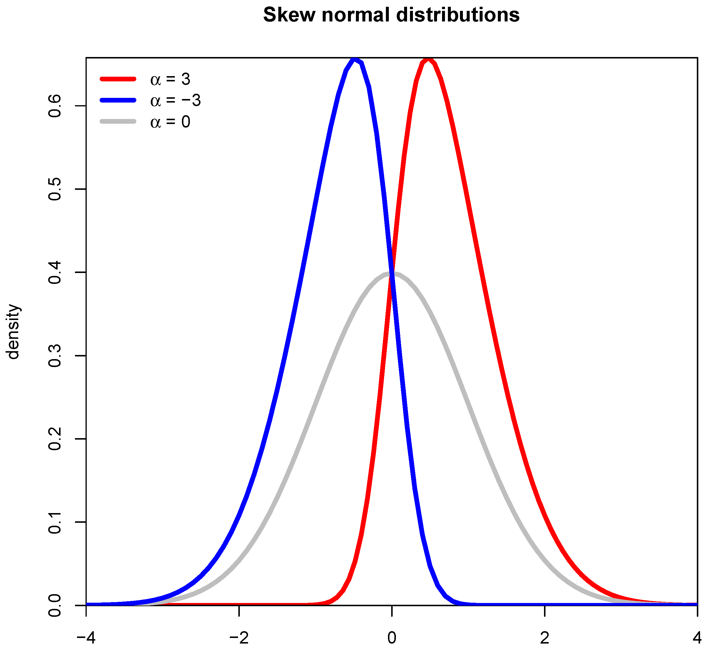
In the following, we use K ( x ; m , s , α ) for the CDF of the skew normal distribution. Note that if α = 0 , we have a Gaussian distribution of mean m and variance s 2 . For m = 0 and s = 1 , the Figure 2 shows the role of α in the skew normal distribution.
The skew normal distribution has a mean and variance, respectively, of
μ = m + s δ 2 π and σ 2 = s 2 1 2 δ 2 π
where δ = α 1 + α 2 is determined from the skewness γ :
δ = γ | γ | π 2 | γ | 2 3 | γ | 2 3 + ( ( 4 π ) / 2 ) 2 3 with γ ( 1 , 1 ) .
The extreme values for α = δ 1 δ 2 are reached when δ 2 is close to 1, which is equivalent to | γ | = 0.99527 . Therefore, the calculation of α is only possible if | γ | is reasonably small. Pewsey [38] reports these issues for the skew normal distribution, where no closed-form expression of the maximum likelihood estimator of ( m , s , α ) is available (unless α = 0 ).
For this study, the representation of the single parametric skew normal distribution is as follows:
m ^ = a 0 + a C T R L C T R L + a E N S ¯ E N S ¯ s ^ δ ^ 2 / π ,
s ^ = b 0 + b E N S σ E N S 1 2 δ ^ 2 / π ,
γ ^ = c 0 + c E N S γ E N S ,
δ ^ = γ ^ | γ ^ | min 0.99 , π 2 | γ ^ | 2 3 | γ ^ | 2 3 + ( ( 4 π ) / 2 ) 2 3 ,
α ^ = δ ^ 1 δ ^ 2 ,
where γ E N S is the empirical ensemble skewness. As for the Gaussian framework, the coefficients a C T R L ,   a E N S ¯ ,   b 0 ,   b E N S are constrained to be non-negative. A formula for the LogS is not hard to compute. Denoting ( ; α ) = ( ; 0 , 1 , α ) for k and K, a closed-form expression of the CRPS is available:
CRPS ( K ( ; α ) , y ) = y [ 2 K ( y ; α ) 1 ] + 2 k ( y ; α ) 2 δ 2 π Φ y α δ + δ 2 π 8 π 3 2 arctan α δ δ arctan α 2
and
CRPS ( K ( ; m , s , α ) , y ) = s CRPS K ( ; α ) , y m s
In the following, the EMOS algorithms using a single skew normal density are called SKN-LOGS and SKN-CRPS.

2.2.3. Mixture Distributions for EMOS

Following the work of Baran and Lerch [28], Möller and Groß [30], we can use a weighted mixture of distributions to exploit the differences between distinguishable components of the ensemble. As mentioned in Baran and Lerch [29], this is different to a combination of predictive distributions where single parametric distributions are determined and then pooled in a two-step procedure where the weights are estimated after. This topic is beyond the scope of the paper, but the interested reader in probabilistic aggregation can refer to Baran and Lerch [29], Ranjan and Gneiting [39], Gneiting et al. [40], Zamo et al. [41]. In this study, two mixtures are proposed. The first one is a mixture of two Gaussian distributions (called MIXNRM-LOGS and MIXNRM-CRPS in the following). The predictive density is
φ ( x ; μ C T R L , σ C T R L , μ E N S ¯ , σ E N S ¯ , ω ) = ω ϕ x μ C T R L σ C T R L σ C T R L + ( 1 ω ) ϕ x μ E N S ¯ σ E N S ¯ σ E N S ¯
where μ C T R L and μ E N S ¯ are affine functions of C T R L and E N S ¯ , respectively. σ C T R L is a non-negative real and σ E N S ¯ is an affine function (with non-negative coefficients) of the ensemble standard deviation σ E N S .
The second mixture proposed relies on a skew normal fit for the distribution of the control run (where the skewness depends on the ensemble skewness) and a Gaussian distribution for the ensemble mean; in terms of predictive density, this yields
ψ ( x ; m C T R L , s , μ E N S ¯ , σ E N S ¯ , α , ω ) = ω k ( x ; m C T R L , s , α ) + ( 1 ω ) ϕ x μ E N S ¯ σ E N S ¯ σ E N S ¯
where μ E N S ¯ is an affine function of E N S ¯ , s is a non-negative real, and σ E N S ¯ is an affine function (with non-negative coefficients) of the ensemble standard deviation σ E N S . α is computed using Equations (7)–(9). m C T R L is calculated with the Equation (5), where, in this case, a E N S ¯ = 0 . Due to the central limit theorem, a Gaussian distribution for the ensemble mean is chosen, the skew normal distribution is fitted using CTRL and ensemble empirical skewness. Grimit et al. [42] provided the closed-form expression of the CRPS for a mixture of Gaussian distributions, and Baran and Lerch [29] provided a formula for a combination of two predictive distributions H ( t ) = w F ( t ) + ( 1 w ) G ( t ) :
CRPS ( H , y ) = w 2 CRPS ( F , y ) + ( 1 w ) 2 CRPS ( G , y ) + 2 w ( 1 w ) ( 1 { x y } F ( x ) ) ( 1 { x y } G ( x ) ) d x .
The last integral term does not have a closed-form for the mixture proposed in (13). As a result, only the mixture MIXSKN-LOGS is considered here.

2.2.4. Training, Tuning, and Link Functions

Recently, Lang et al. [43] examined the training strategies for nonhomogeneous regression. A trade-off is made between time adaptation and the data over multiple years to obtain unbiased and stable regression estimates. Here, the choice is made to adjust the coefficients seasonally using all of the same seasons available in the data set. More precisely, each year is divided into four seasons of three months, and the coefficients estimated for a season with two given years are applied to the third year to compute the predictive distributions.
Both maximum likelihood (LogS) estimation and CRPS minimization are used when possible. Gebetsberger et al. [44], Yuen and Stoev [45] notice that these estimations yield similar results when the response distribution is well specified, which is natural since one can guess that the minimum expected values of the scores are reached; thus, the ideal forecast is made, according to the definition of proper scoring rules. Using various estimation methods permits detecting model misspecification implicitly. Practically, one must avoid overfitting. For example, in case the coefficients are estimated day by day, Scheuerer [46] proposes to stop the optimization early provided that starting values are known to be accurate. The question of numerical optimization is a crucial one when dealing with a huge number of models where a manual check of the coefficients is hard to do. Gebetsberger et al. [47] report some solutions to avoid numerical blow up, for example, the use of the quadratic link function for non-negative coefficients [15]. Moreover, the LogS and the CRPS are not sensitive to the same errors in numerical optimization and Gneiting et al. [15] states that a LogS strategy can lead to overdispersed forecasts and CRPS can lead to sharper but lesser calibrated forecasts [44].
Hence, a universal link function is proposed here, for a parameter θ , based on the logistic function:
l ( θ ; A , B ) = A + B e θ 1 + e θ
The function l ( ; A , B ) is defined on R so no constrained estimation is imposed. In addition, the link function is bounded on ( A , B ) and the range of the coefficients can be controlled. Last but not least, the derivatives of l ( ; A , B ) are mild and easy to compute. The spirit here is very similar to the use of sigmoid functions in neural networks, leading to faster convergence with backpropagation [48].
For instance, in the three mixture EMOSs exposed, all three use l ( ; 0.05 , 0.95 ) to represent ω . A summary of the link functions employed according to the methods used is available in Table 1.

3. Results

All results presented in the following come from 3-fold cross-validation based on the 3 years of data at hand. For each station, lead time, and season, three regression models are estimated using two seasons while the remaining season is used for validation. In the following, the raw ensemble is denoted by RAW. For the postprocessed methods, quantiles of order 1 52 , 2 52 , , 51 52 are computed and used in the verification process.

Probabilistic Calibration

Probabilistic calibration is commonly evaluated with probability integral transform (PIT) or rank histograms (RH) [49,50,51,52]. Subject to calibration, the PIT statistic follows a uniform distribution, its mean is 1 2 , and its normalized variance is 1 [3,53]. Figure 3 summarizes PIT mean and variance on the 2056 weather stations.
The PIT mean shows a clear improvement of forecast bias regardless of the method considered. The RAW ensemble is cold-biased, and the diurnal effect on forecast performance is reduced. The PIT variance of the RAW indicates an underdispersed forecast, with a reduction of the underdispersion across lead times. It may be imputable to the inflation of the spread of the ensemble. Most of the LogS-learned algorithms show a very slight overdispersion, especially for earlier lead times. NORM-CRPS and SKN-LOGS have an increase of the PIT variance across lead times, until the RAW PIT variance. Moreover, SKN-CRPS clearly shows underdispersed forecasts, with its best dispersion from Day 4 to Day 6. The stability of the behavior of MIXNRM indicates that a fit of Gaussian mixture is a good specification for ensemble forecasts of temperature. NORM-CRPS probably indicates that a normal fit, for longer lead times, is unable to catch enough variability from the RAW distribution. The bad dispersion of SKN-CRPS may come from a target distribution, which is not tailored for a single parametric EMOS for temperature or for an erratic management of forecast variance by the CRPS itself—the LogS being more sensitive to dispersion issues. At last, it is interesting to see that SKN and NORM have different predictive patterns even if the Gaussian distribution is a special case of the skew normal distribution.
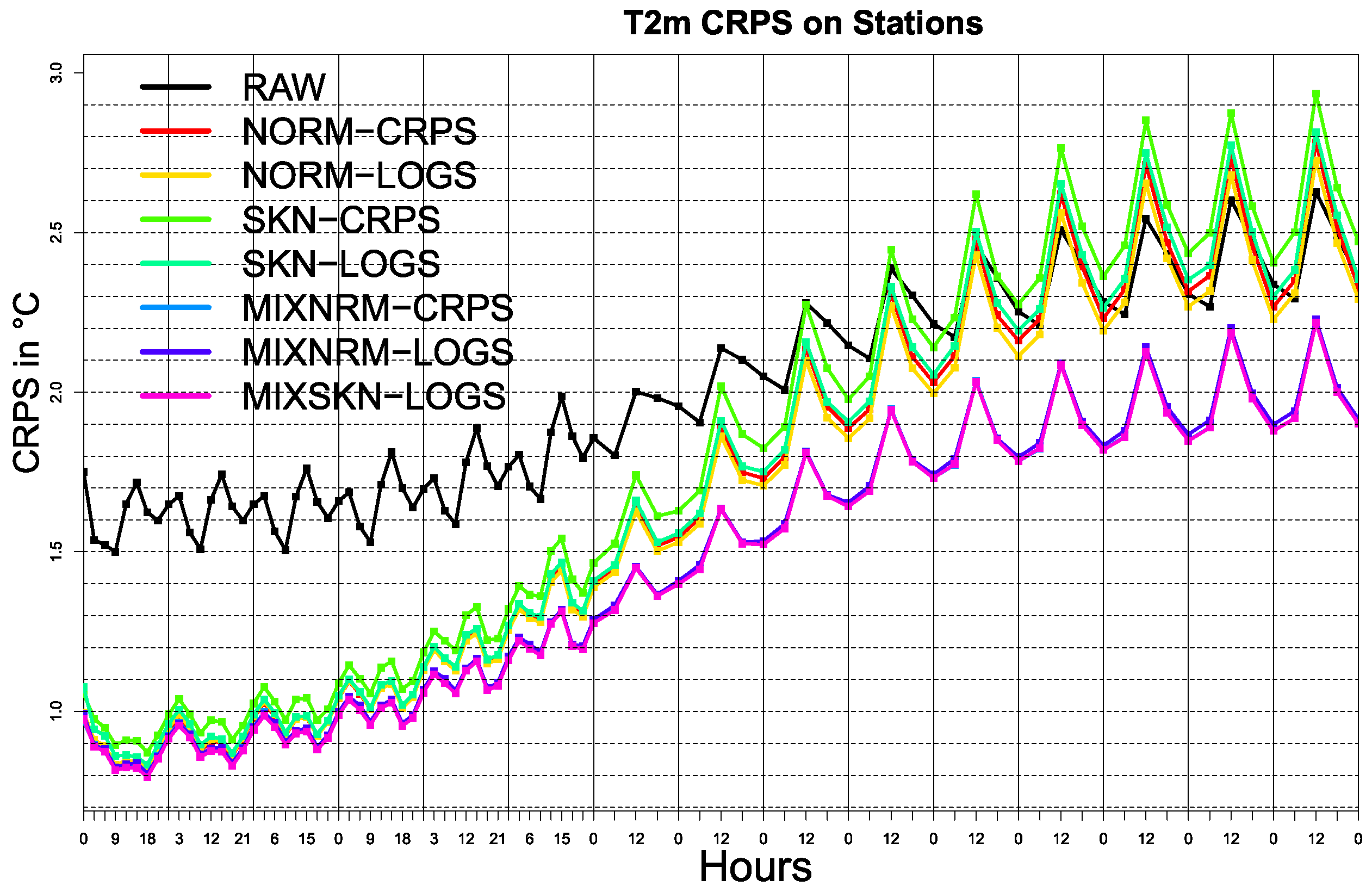
Figure 4 represents the average CRPS for each technique along lead times. The CRPS are computed using the 51-quantile forecasts issued from the predictive distributions and following Hersbach [36], Ferro [54], Zamo and Naveau [55]. Single parametric EMOS have a performance similar to the RAW ensemble at Day 10, and the CRPSS (skill score—not shown here) with respect to the raw ensemble are below 0 after Day 10. The EMOS method is not to blame; however, these results can be explained by the lack of information on the RAW ensemble (not enough covariates) and predictive distributions that are not flexible enough. The results until Day 10 are in compliance with Hemri et al. [56]. The three MIX models are very close together and have the best CRPS averages, especially from Day 6, showing the importance of a mixture representation of ensemble forecasts of temperature; in this case, their CRPSS are at 0.4 near Day 1, and fall down to 0.2 at Day 15. Notice that the SKN-CRPS seems to be the worst postprocessed forecast but one found that misdispersion (here, sharper but lesser calibrated forecasts) is hidden by the CRPS, which confirms the finding of Gebetsberger et al. [44].
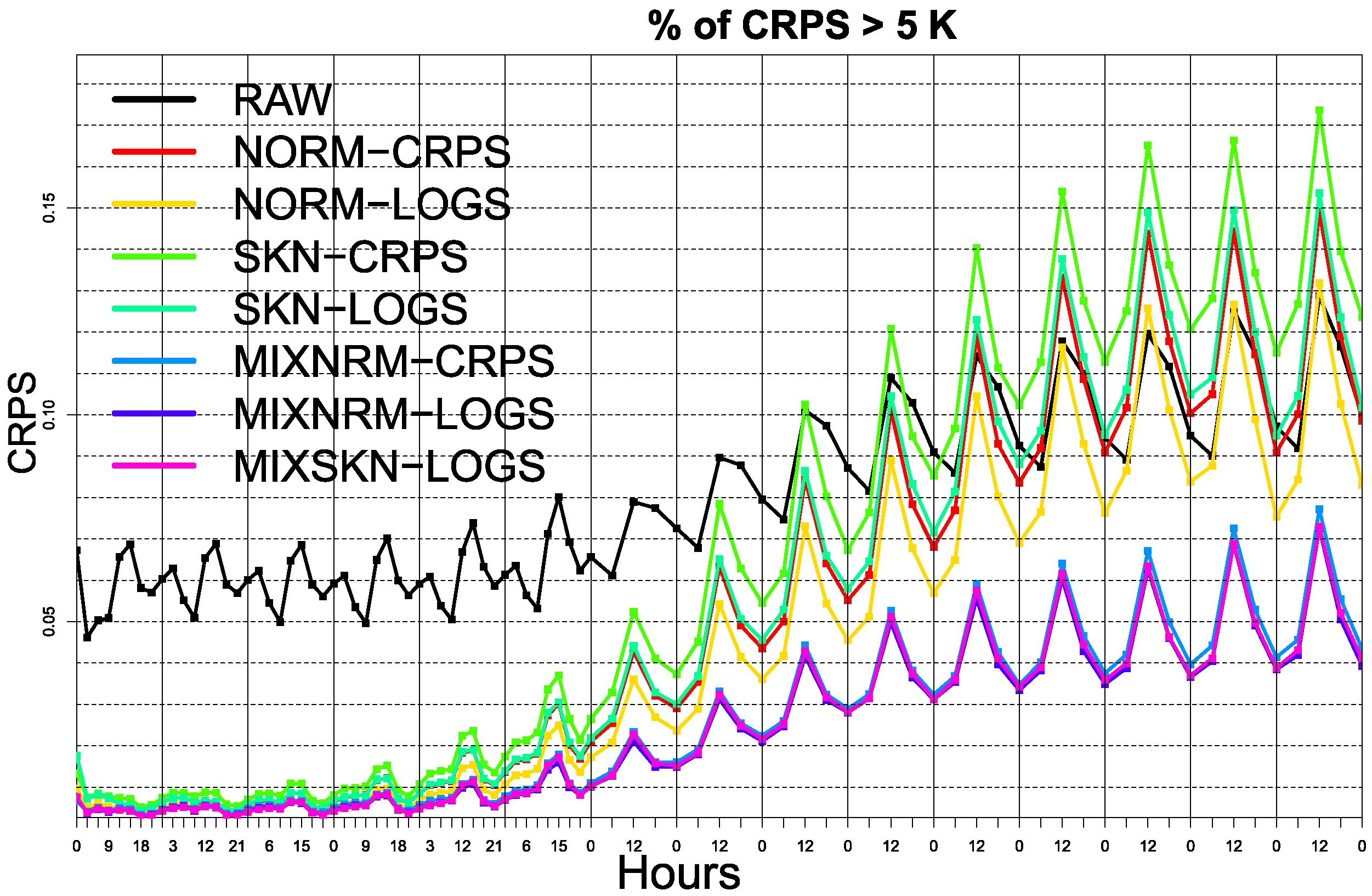
The ECMWF use a new headline index based on the percentage of “large errors”, i.e., forecasts, where CRPS > 5 °C at Day 5 [57]. This idea is taken here and exposed in Figure 5.
Figure 5 is very similar to Figure 4. There is a clear improvement of the large errors, especially with the mixture models and after Day 10. However, it is noteworthy that for the single parametric EMOS, the LogS-learned methods commit less large errors than with a CRPS optimization. This behavior is quite logical since CRPS provides sharper forecasts; however, here, it is too confident with respect to the forecast horizon.
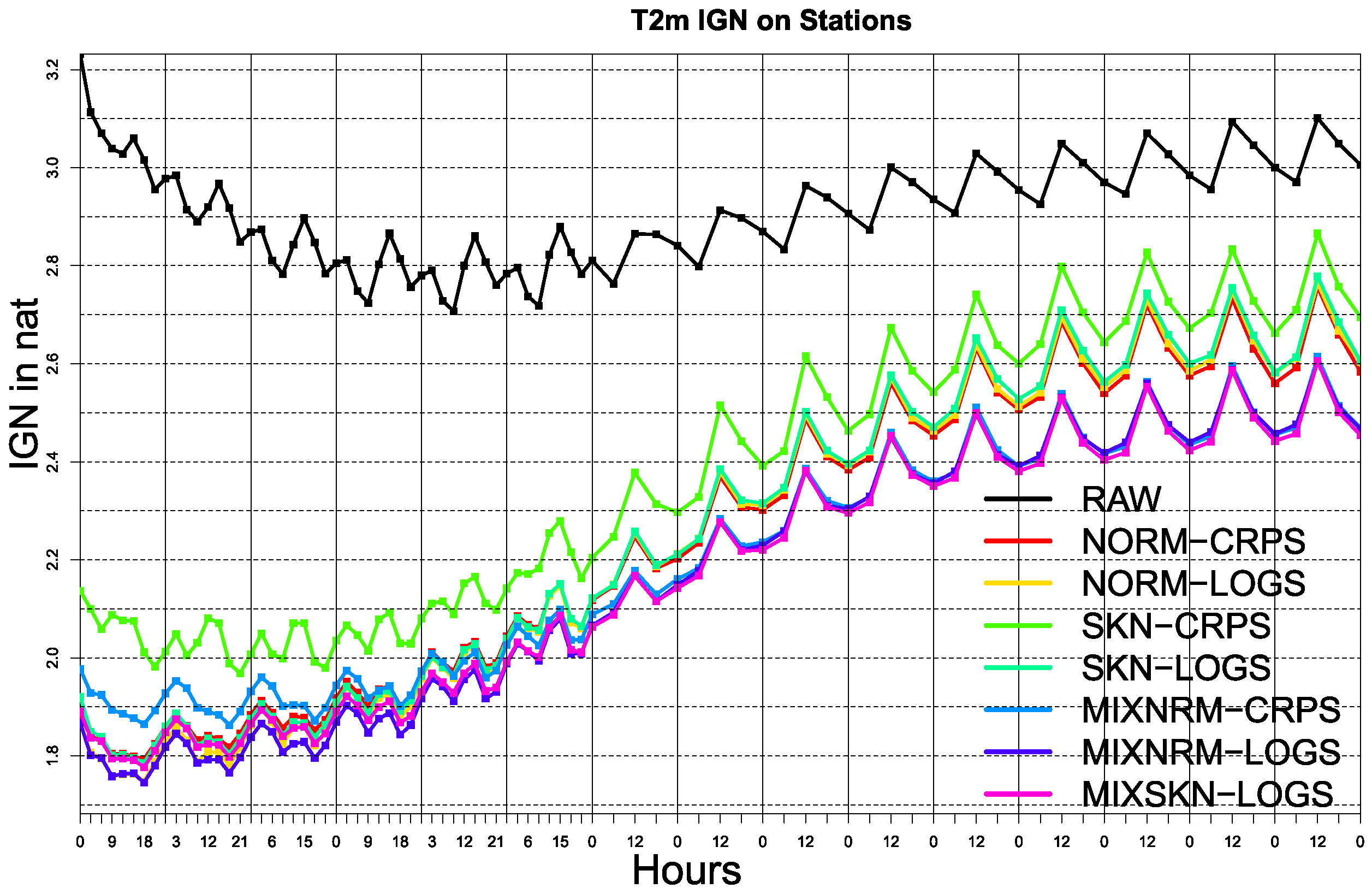
In order to understand the differences between optimization strategies, an assessment of forecast quality using the LogS is presented in Figure 6. The choice is made to work with the ensemble members instead of the predictive distribution to be fair with the RAW ensemble. A discretization of the LogS is made in the spirit of Roulston and Smith [34] proposal. Let f 1 , , f 51 be the ordered (and rounded to the closest tenth) values of the predictive distribution, the LogS ( f , y ) (in nat) proposed is
LogS ( f , y ) = log ( 51 ) + log ( max ( 0.05 , f 1 y ) ) if y f 1 log ( 51 ) + log ( max ( 0.05 , f j + 1 f j ) ) if f j y f j + 1 log ( 51 ) + log ( max ( 0.05 , y f 51 ) ) if y f 51
where the lower the better. Here, one must be careful regarding the sensitivity of the inference of the score above. Indeed, some choices can interfere with our results here. The interested reader on this topic can consult Weijs et al. [58], Tödter and Ahrens [59], Siegert et al. [60].
First, one can assume that the ranking of the forecasts is very similar to those in Figure 4; in particular, for the best method at each lead time. Using proper scoring rules in verification ensures that the best (but a priori unknown) forecasts are rewarded on average. Here, the fact that the same forecast (MIXNRM-LOGS) seems to be dominant both in CRPS and LogS advocates that this forecast is the best subject for the information provided by the RAW ensemble (i.e., the score has only an uncertainty component remaining). Yet, a difference between MIXNRM-LOGS and MIXNRM-CRPS is noticeable until Day 3, and the SKN-CRPS method is still the worst among postprocessed forecasts. In contrast to Figure 3, the LogS seems to penalize underdispersed forecasts, as in the optimization process. Last but not least, the RAW ensemble seems to gain predictive performance until Day 6. This is not the case in Figure 4. This can be due to the initial ensemble perturbations of the RAW ensemble [61], probably better tailored to medium-range or extended-range forecasts.
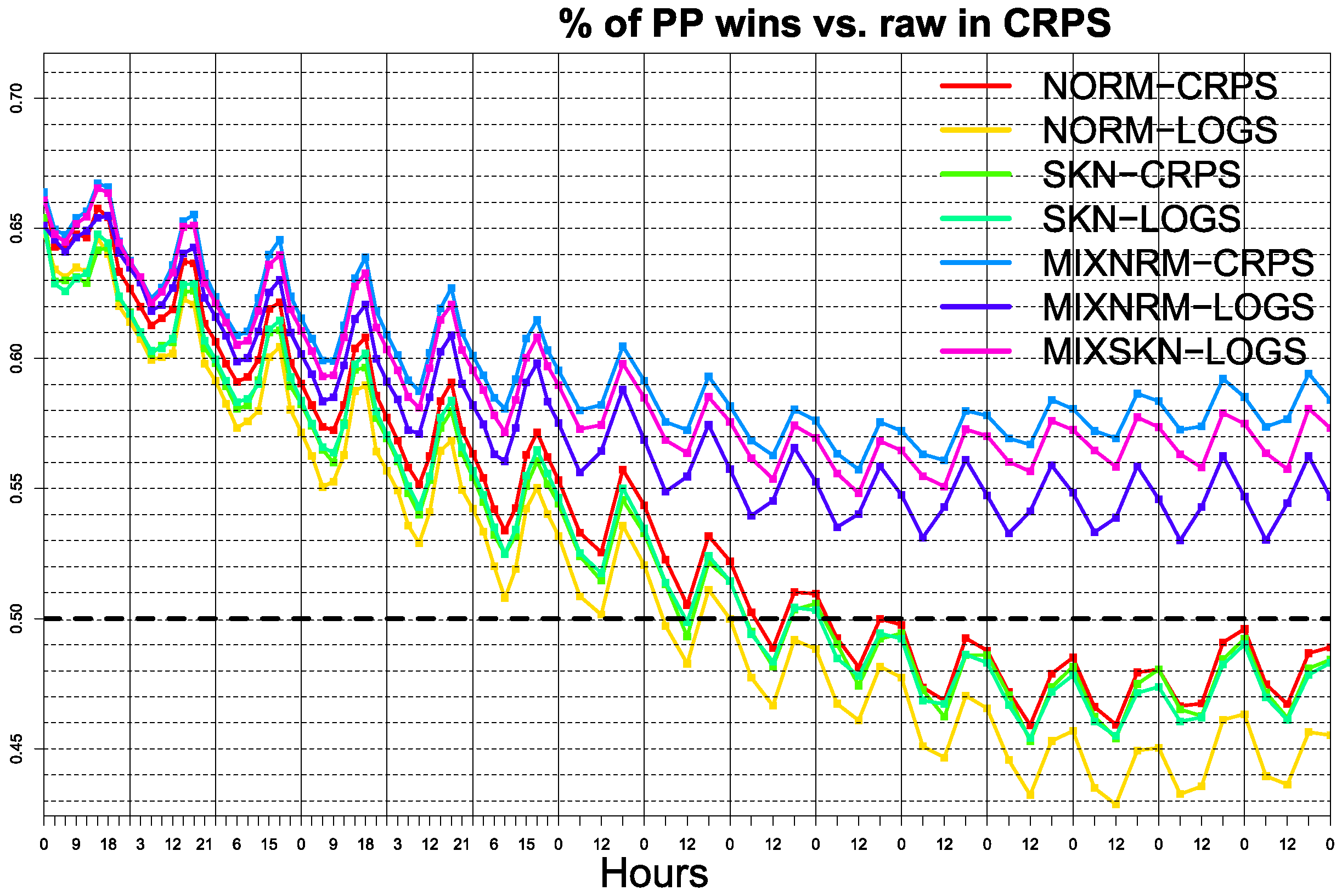
The differences between MIXNRM-LOGS, MIXNRM-CRPS, and MIXSKN-LOGS are not very significant in terms of scoring rules. Therefore, the final choice of a predictive distribution can be made using a simple tool inspired by the so-called weather roulette [62]. Figure 7 shows the frequency where the CRPS of the postprocessed forecast is better than the RAW forecast. This tool demonstrates that the MIXNRM-CRPS wins 1 % more than the other methods against the RAW ensemble for the longest lead times.

4. Discussion and Conclusions

Overall, all the postprocessed forecasts show an improvement compared to the RAW ensemble. The single parametric distributions are effective until Day 10. The mixture distributions are the most skillful forecasts, regardless of the forecast horizon. This statement is supported through two different proper scoring rules, emphasizing and penalizing different types of errors. We are unaware of the connections of the tool of Figure 7 with some tests of predictive performance, economic value of the forecasts, or scoring rules, and such a figure should be drawn for LogS. In the future, very simple ideas such as “Your forecast is better than the RAW one X times over Y” would be in favor of a broader communication of ensemble information for decision making [63].
The choice of a “perfect” parametric distribution is probably a never-ending story. The mixture distributions are appealing solutions to overcome this issue. Here, the skew normal distribution is probably not tailored for a single parametric use and/or for surface temperature ensemble forecasts. Skewed distributions propose new solutions in order to combine nonexchangeable forecasts with distributions centered on ensemble means. In this study, the skew normal distributions are applied on the control forecast but one may consider other ensemble forecasts to combine. Moreover, more and more meteorological variables are postprocessed with numerous distributions, see e.g., Schulz et al. [64], Baran et al. [65]; in this context, the more distributions one tries, the better the results will be. For future work, one may try to implement EMOS schemes where the choice of a parametric distribution is related on forecasted weather regimes.
In all cases, the choice of appropriate parameter estimation schemes and link functions appears to be as important as the choice of target distributions. It is not shown here, but one finds that the proportion of Normality tests rejected across lead times is clearly anticorrelated to the RAW LogS, and that tests relying on Kolmogorov–Smirnov statistic are less powerful than Jarque–Bera or Shapiro–Wilk ones. The Kolmogorov–Smirnov statistic is based on a CDF distance such as the CRPS. One can wonder whether this behavior is to associate with the better sensitivity of the CRPS than the LogS to tolerate misspecification but it upholds the work of Leutbecher and Haiden [66] on a Gaussian approximation of the CRPS.
This work is also an advocate for the use of several scoring rules in forecast verification. Some scores, even if they are proper, are sensitive to different types of forecast errors, and differences among them can pinpoint peculiarities in forecasts. Indeed, minimizing an expected score may be less important than reducing large (and costly) errors.

Funding

Part of this work was supported by the French National Research Agency (ANR) project T-REX (ANR-20-CE40-0025) and by Energy oriented Centre of Excellence-II (EoCoE-II), Grant Agreement 824158, funded within the Horizon2020 framework of the European Union.

Institutional Review Board Statement

Not applicable.

Informed Consent Statement

Not applicable.

Data Availability Statement

Observation data and sketches of EMOS codes are available upon request to the author. The ECMWF ensemble is available on TIGGE [67]. TIGGE (The Interactive Grand Global Ensemble) is an initiative of the World Weather Research Programme (WWRP).

Acknowledgments

The author thanks the three anonymous reviewers for their helpful comments and suggestions.

Conflicts of Interest

The author declares no conflict of interest.

References

  1. Leith, C. Theoretical skill of Monte Carlo forecasts. Mon. Weather Rev. 1974, 102, 409–418. [Google Scholar] [CrossRef] [Green Version]
  2. Palmer, T. The economic value of ensemble forecasts as a tool for risk assessment: From days to decades. Q. J. R. Meteorol. Soc. 2002, 128, 747–774. [Google Scholar] [CrossRef]
  3. Gneiting, T.; Katzfuss, M. Probabilistic forecasting. Annu. Rev. Stat. Its Appl. 2014, 1, 125–151. [Google Scholar] [CrossRef]
  4. Bauer, P.; Thorpe, A.; Brunet, G. The quiet revolution of numerical weather prediction. Nature 2015, 525, 47–55. [Google Scholar] [CrossRef]
  5. Vannitsem, S.; Wilks, D.S.; Messner, J. Statistical Postprocessing of Ensemble Forecasts; Elsevier: Amsterdam, The Netherlands, 2018. [Google Scholar]
  6. Vannitsem, S.; Bremnes, J.B.; Demaeyer, J.; Evans, G.R.; Flowerdew, J.; Hemri, S.; Lerch, S.; Roberts, N.; Theis, S.; Atencia, A.; et al. Statistical Postprocessing for Weather Forecasts: Review, Challenges, and Avenues in a Big Data World. Bull. Am. Meteorol. Soc. 2021, 102, E681–E699. [Google Scholar] [CrossRef]
  7. Haupt, S.E.; Chapman, W.; Adams, S.V.; Kirkwood, C.; Hosking, J.S.; Robinson, N.H.; Lerch, S.; Subramanian, A.C. Towards implementing artificial intelligence post-processing in weather and climate: Proposed actions from the Oxford 2019 workshop. Philos. Trans. R. Soc. A 2021, 379, 20200091. [Google Scholar] [CrossRef]
  8. Taillardat, M.; Mestre, O.; Zamo, M.; Naveau, P. Calibrated ensemble forecasts using quantile regression forests and ensemble model output statistics. Mon. Weather Rev. 2016, 144, 2375–2393. [Google Scholar] [CrossRef]
  9. Rasp, S.; Lerch, S. Neural networks for post-processing ensemble weather forecasts. arXiv 2018, arXiv:1805.09091. [Google Scholar]
  10. Scheuerer, M.; Switanek, M.B.; Worsnop, R.P.; Hamill, T.M. Using Artificial Neural Networks for Generating Probabilistic Subseasonal Precipitation Forecasts over California. Mon. Weather Rev. 2020, 148, 3489–3506. [Google Scholar] [CrossRef]
  11. Veldkamp, S.; Whan, K.; Dirksen, S.; Schmeits, M. Statistical postprocessing of wind speed forecasts using convolutional neural networks. Mon. Weather Rev. 2021, 149, 1141–1152. [Google Scholar] [CrossRef]
  12. Grönquist, P.; Yao, C.; Ben-Nun, T.; Dryden, N.; Dueben, P.; Li, S.; Hoefler, T. Deep learning for post-processing ensemble weather forecasts. Philos. Trans. R. Soc. A 2021, 379, 20200092. [Google Scholar] [CrossRef]
  13. Hess, R. Statistical postprocessing of ensemble forecasts for severe weather at Deutscher Wetterdienst. Nonlinear Process. Geophys. 2020, 27, 473–487. [Google Scholar] [CrossRef]
  14. Taillardat, M.; Mestre, O. From research to applications—Examples of operational ensemble post-processing in France using machine learning. Nonlinear Process. Geophys. 2020, 27, 329–347. [Google Scholar] [CrossRef]
  15. Gneiting, T.; Raftery, A.E.; Westveld III, A.H.; Goldman, T. Calibrated probabilistic forecasting using ensemble model output statistics and minimum CRPS estimation. Mon. Weather Rev. 2005, 133, 1098–1118. [Google Scholar] [CrossRef]
  16. Hagedorn, R.; Hamill, T.M.; Whitaker, J.S. Probabilistic forecast calibration using ECMWF and GFS ensemble reforecasts. Part I: Two-meter temperatures. Mon. Weather Rev. 2008, 136, 2608–2619. [Google Scholar] [CrossRef]
  17. Thorarinsdottir, T.L.; Gneiting, T. Probabilistic forecasts of wind speed: Ensemble model output statistics by using heteroscedastic censored regression. J. R. Stat. Soc. Ser. A (Stat. Soc.) 2010, 173, 371–388. [Google Scholar] [CrossRef]
  18. Baran, S.; Lerch, S. Log-normal distribution based Ensemble Model Output Statistics models for probabilistic wind-speed forecasting. Q. J. R. Meteorol. Soc. 2015, 141, 2289–2299. [Google Scholar] [CrossRef] [Green Version]
  19. Scheuerer, M.; Hamill, T.M. Statistical postprocessing of ensemble precipitation forecasts by fitting censored, shifted gamma distributions. Mon. Weather Rev. 2015, 143, 4578–4596. [Google Scholar] [CrossRef]
  20. Friederichs, P.; Thorarinsdottir, T.L. Forecast verification for extreme value distributions with an application to probabilistic peak wind prediction. Environmetrics 2012, 23, 579–594. [Google Scholar] [CrossRef] [Green Version]
  21. Friederichs, P.; Göber, M.; Bentzien, S.; Lenz, A.; Krampitz, R. A probabilistic analysis of wind gusts using extreme value statistics. Meteorol. Z. 2009, 18, 615–629. [Google Scholar] [CrossRef]
  22. Jordan, A.; Krüger, F.; Lerch, S. Evaluating Probabilistic Forecasts with scoringRules. J. Stat. Softw. 2019, 90, 1–37. [Google Scholar] [CrossRef] [Green Version]
  23. Messner, J.W.; Mayr, G.J.; Zeileis, A. Nonhomogeneous Boosting for Predictor Selection in Ensemble Postprocessing. Mon. Weather Rev. 2017, 145, 137–147. [Google Scholar] [CrossRef] [Green Version]
  24. Junk, C.; Delle Monache, L.; Alessandrini, S. Analog-based ensemble model output statistics. Mon. Weather Rev. 2015, 143, 2909–2917. [Google Scholar] [CrossRef]
  25. Feldmann, K.; Scheuerer, M.; Thorarinsdottir, T.L. Spatial postprocessing of ensemble forecasts for temperature using nonhomogeneous Gaussian regression. arXiv 2014, arXiv:1407.0058. [Google Scholar] [CrossRef] [Green Version]
  26. Dabernig, M.; Mayr, G.J.; Messner, J.W.; Zeileis, A. Spatial Ensemble Post-Processing with Standardized Anomalies. Q. J. R. Meteorol. Soc. 2016, 143, 909–916. [Google Scholar] [CrossRef] [Green Version]
  27. Gebetsberger, M.; Stauffer, R.; Mayr, G.J.; Zeileis, A. Skewed logistic distribution for statistical temperature post-processing in mountainous areas. Adv. Stat. Climatol. Meteorol. Oceanogr. 2019, 5, 87–100. [Google Scholar] [CrossRef]
  28. Baran, S.; Lerch, S. Mixture EMOS model for calibrating ensemble forecasts of wind speed. Environmetrics 2016, 27, 116–130. [Google Scholar] [CrossRef] [Green Version]
  29. Baran, S.; Lerch, S. Combining predictive distributions for the statistical post-processing of ensemble forecasts. Int. J. Forecast. 2018, 34, 477–496. [Google Scholar] [CrossRef] [Green Version]
  30. Möller, A.; Groß, J. Probabilistic temperature forecasting based on an ensemble autoregressive modification. Q. J. R. Meteorol. Soc. 2016, 142, 1385–1394. [Google Scholar] [CrossRef] [Green Version]
  31. Raftery, A.E.; Gneiting, T.; Balabdaoui, F.; Polakowski, M. Using Bayesian model averaging to calibrate forecast ensembles. Mon. Weather Rev. 2005, 133, 1155–1174. [Google Scholar] [CrossRef] [Green Version]
  32. Mureau, R.; Molteni, F.; Palmer, T. Ensemble prediction using dynamically conditioned perturbations. Q. J. R. Meteorol. Soc. 1993, 119, 299–323. [Google Scholar] [CrossRef]
  33. Gneiting, T. Calibration of Medium-Range Weather Forecasts; European Centre for Medium-Range Weather Forecasts: Reading, UK, 2014. [Google Scholar]
  34. Roulston, M.S.; Smith, L.A. Evaluating probabilistic forecasts using information theory. Mon. Weather Rev. 2002, 130, 1653–1660. [Google Scholar] [CrossRef] [Green Version]
  35. Matheson, J.E.; Winkler, R.L. Scoring rules for continuous probability distributions. Manag. Sci. 1976, 22, 1087–1096. [Google Scholar] [CrossRef]
  36. Hersbach, H. Decomposition of the continuous ranked probability score for ensemble prediction systems. Weather Forecast. 2000, 15, 559–570. [Google Scholar] [CrossRef]
  37. Gneiting, T.; Raftery, A.E. Strictly proper scoring rules, prediction, and estimation. J. Am. Stat. Assoc. 2007, 102, 359–378. [Google Scholar] [CrossRef]
  38. Pewsey, A. Problems of inference for Azzalini’s skewnormal distribution. J. Appl. Stat. 2000, 27, 859–870. [Google Scholar] [CrossRef]
  39. Ranjan, R.; Gneiting, T. Combining probability forecasts. J. R. Stat. Soc. Ser. B (Stat. Methodol.) 2010, 72, 71–91. [Google Scholar] [CrossRef] [Green Version]
  40. Gneiting, T.; Ranjan, R. Combining predictive distributions. Electron. J. Stat. 2013, 7, 1747–1782. [Google Scholar] [CrossRef]
  41. Zamo, M.; Bel, L.; Mestre, O. Sequential aggregation of probabilistic forecasts—Application to wind speed ensemble forecasts. J. R. Stat. Soc. Ser. C (Appl. Stat.) 2021, 70, 202–225. [Google Scholar] [CrossRef]
  42. Grimit, E.P.; Gneiting, T.; Berrocal, V.; Johnson, N.A. The Continuous Ranked Probability Score for Circular Variables and Its Application to Mesoscale Forecast Ensemble Verification; Technical Report; DTIC Document: Bedford, MA, USA, 2006. [Google Scholar]
  43. Lang, M.N.; Lerch, S.; Mayr, G.J.; Simon, T.; Stauffer, R.; Zeileis, A. Remember the past: A comparison of time-adaptive training schemes for non-homogeneous regression. Nonlinear Process. Geophys. 2020, 27, 23–34. [Google Scholar] [CrossRef] [Green Version]
  44. Gebetsberger, M.; Messner, J.W.; Mayr, G.J.; Zeileis, A. Estimation methods for nonhomogeneous regression models: Minimum continuous ranked probability score versus maximum likelihood. Mon. Weather Rev. 2018, 146, 4323–4338. [Google Scholar] [CrossRef]
  45. Yuen, R.; Stoev, S. CRPS M-estimation for max-stable models. Extremes 2014, 17, 387–410. [Google Scholar] [CrossRef] [Green Version]
  46. Scheuerer, M. Probabilistic quantitative precipitation forecasting using ensemble model output statistics. Q. J. R. Meteorol. Soc. 2014, 140, 1086–1096. [Google Scholar] [CrossRef] [Green Version]
  47. Gebetsberger, M.; Messner, J.W.; Mayr, G.J.; Zeileis, A. Fine-tuning nonhomogeneous regression for probabilistic precipitation forecasts: Unanimous predictions, heavy tails, and link functions. Mon. Weather Rev. 2017, 145, 4693–4708. [Google Scholar] [CrossRef] [Green Version]
  48. LeCun, Y.A.; Bottou, L.; Orr, G.B.; Müller, K.R. Efficient backprop. In Neural Networks: Tricks of the Trade; Springer: Berlin/Heidelberg, Germany, 2012; pp. 9–48. [Google Scholar]
  49. Gneiting, T.; Balabdaoui, F.; Raftery, A.E. Probabilistic forecasts, calibration and sharpness. J. R. Stat. Soc. Ser. B (Stat. Methodol.) 2007, 69, 243–268. [Google Scholar] [CrossRef] [Green Version]
  50. Anderson, J.L. A method for producing and evaluating probabilistic forecasts from ensemble model integrations. J. Clim. 1996, 9, 1518–1530. [Google Scholar] [CrossRef]
  51. Talagrand, O.; Vautard, R.; Strauss, B. Evaluation of probabilistic prediction systems. In Proceedings of the ECMWF Workshop on Predictability, Reading, UK, 20–22 October 1997; pp. 1–25. [Google Scholar]
  52. Hamill, T.M.; Colucci, S.J. Verification of Eta-RSM short-range ensemble forecasts. Mon. Weather Rev. 1997, 125, 1312–1327. [Google Scholar] [CrossRef]
  53. Taillardat, M.; Fougères, A.L.; Naveau, P.; Mestre, O. Forest-based and semiparametric methods for the postprocessing of rainfall ensemble forecasting. Weather Forecast. 2019, 34, 617–634. [Google Scholar] [CrossRef]
  54. Ferro, C. Fair scores for ensemble forecasts. Q. J. R. Meteorol. Soc. 2014, 140, 1917–1923. [Google Scholar] [CrossRef] [Green Version]
  55. Zamo, M.; Naveau, P. Estimation of the continuous ranked probability score with limited information and applications to ensemble weather forecasts. Math. Geosci. 2018, 50, 209–234. [Google Scholar] [CrossRef] [Green Version]
  56. Hemri, S.; Scheuerer, M.; Pappenberger, F.; Bogner, K.; Haiden, T. Trends in the predictive performance of raw ensemble weather forecasts. Geophys. Res. Lett. 2014, 41, 9197–9205. [Google Scholar] [CrossRef]
  57. Haiden, T.; Janousek, M.; Bidlot, J.; Buizza, R.; Ferranti, L.; Prates, F.; Vitart, F. Evaluation of ECMWF Forecasts, Including the 2018 Upgrade; European Centre for Medium Range Weather Forecasts: Reading, UK, 2018. [Google Scholar]
  58. Weijs, S.V.; Van Nooijen, R.; Van De Giesen, N. Kullback–Leibler divergence as a forecast skill score with classic reliability–resolution–uncertainty decomposition. Mon. Weather Rev. 2010, 138, 3387–3399. [Google Scholar] [CrossRef]
  59. Tödter, J.; Ahrens, B. Generalization of the ignorance score: Continuous ranked version and its decomposition. Mon. Weather Rev. 2012, 140, 2005–2017. [Google Scholar] [CrossRef]
  60. Siegert, S.; Ferro, C.A.; Stephenson, D.B.; Leutbecher, M. The ensemble-adjusted Ignorance Score for forecasts issued as normal distributions. Q. J. R. Meteorol. Soc. 2019, 145, 129–139. [Google Scholar] [CrossRef] [Green Version]
  61. Palmer, T. The ECMWF ensemble prediction system: Looking back (more than) 25 years and projecting forward 25 years. Q. J. R. Meteorol. Soc. 2019, 145, 12–24. [Google Scholar] [CrossRef] [Green Version]
  62. Hagedorn, R.; Smith, L.A. Communicating the value of probabilistic forecasts with weather roulette. Meteorol. Appl. J. Forecast. Pract. Appl. Train. Tech. Model. 2009, 16, 143–155. [Google Scholar] [CrossRef]
  63. Fundel, V.J.; Fleischhut, N.; Herzog, S.M.; Göber, M.; Hagedorn, R. Promoting the use of probabilistic weather forecasts through a dialogue between scientists, developers and end-users. Q. J. R. Meteorol. Soc. 2019, 145, 210–231. [Google Scholar] [CrossRef] [Green Version]
  64. Schulz, B.; El Ayari, M.; Lerch, S.; Baran, S. Post-processing numerical weather prediction ensembles for probabilistic solar irradiance forecasting. Sol. Energy 2021, 220, 1016–1031. [Google Scholar] [CrossRef]
  65. Baran, S.; Szokol, P.; Szabó, M. Truncated generalized extreme value distribution-based ensemble model output statistics model for calibration of wind speed ensemble forecasts. Environmetrics 2021, e2678. [Google Scholar] [CrossRef]
  66. Leutbecher, M.; Haiden, T. Understanding changes of the continuous ranked probability score using a homogeneous Gaussian approximation. Q. J. R. Meteorol. Soc. 2021, 147, 425–442. [Google Scholar] [CrossRef]
  67. Swinbank, R.; Kyouda, M.; Buchanan, P.; Froude, L.; Hamill, T.M.; Hewson, T.D.; Keller, J.H.; Matsueda, M.; Methven, J.; Pappenberger, F.; et al. The TIGGE project and its achievements. Bull. Am. Meteorol. Soc. 2016, 97, 49–67. [Google Scholar] [CrossRef]
Figure 1. Location of the 2056 stations of this study.
Atmosphere 12 00966 g001
Figure 2. Standard skew normal densities ( m = 0 and s = 1 ) as a function of the parameter α .
Atmosphere 12 00966 g002
Figure 3. PIT mean and PIT variance for the 2056 weather stations of the benchmark. Subject to calibration, the PIT statistic follows a uniform distribution, its mean is 1 2 , and its normalized variance is 1.
Atmosphere 12 00966 g003
Figure 4. Average CRPS on 3 years/2056 stations along lead times. The three MIX models are very close together and have the best CRPS averages, especially from Day 6.
Atmosphere 12 00966 g004
Figure 5. Percentage of CRPS (for each day/station) larger than 5 °C along lead times. There is a clear improvement of the large errors, especially with the mixture models and after Day 10.
Atmosphere 12 00966 g005
Figure 6. Average LogS on 3 years/2056 stations along lead times. The ranking of the forecasts is very similar to Figure 4. The RAW ensemble seems to gain predictive performance until Day 6.
Atmosphere 12 00966 g006
Figure 7. Proportion of the cases where the CRPS of the postprocessed forecasts are better than the RAW forecast. This tool demonstrates that the MIXNRM-CRPS wins 1 % more than the other methods against the RAW ensemble for the longest lead times.
Atmosphere 12 00966 g007
Table 1. Summary of the link functions used for parameter estimation.
NORM-CRPSNORM-LOGSSKN-CRPSSKN-LOGS
a C T R L quadraticquadraticquadraticquadratic
a E N S ¯ quadraticquadraticquadraticquadratic
b 0 quadratic l ( ; 0.2 , 1 ) quadratic l ( ; 0.2 , 1 )
b E N S quadratic l ( ; 0.75 , 1.8 ) quadratic l ( ; 0.75 , 2.5 )
MIXNRM-CRPSMIXNRM-LOGSMIXSKN-LOGS
μ C T R L = a 0 + a C T R L C T R L m = a 0 + a C T R L C T R L s δ 2 / π
a C T R L identity l ( ; 0.75 , 1.25 ) l ( ; 0.75 , 1.25 )
μ E N S ¯ = a 0 + a E N S ¯ E N S ¯
a E N S ¯ identity l ( ; 0.75 , 1.25 ) l ( ; 0.75 , 1.25 )
σ C T R L l ( ; 0.1 , 3 ) l ( ; 0.1 , 3 ) -
s-- l ( ; 0.1 , 3 )
σ E N S ¯ = b 0 + b E N S σ E N S
b 0 quadratic l ( ; 0.1 , 2 ) l ( ; 0.1 , 2 )
b E N S quadratic l ( ; 0.8 , 1.3 ) l ( ; 0.8 , 1.3 )
Publisher’s Note: MDPI stays neutral with regard to jurisdictional claims in published maps and institutional affiliations.