Towards Possible Laminar Channels through Turbulent Atmospheres in a Multifractal Paradigm

Abstract

In this paper, developments are made towards simulating complex atmospheric behavior using turbulent energy cascade staging models developed through scale relativity theories. Such theoretical considerations imply gauges that describe atmospheric parameters as multifractal functions undertaking scale symmetry breaking at each stage of the turbulent energy cascade. It is found that gauges of higher complexity (in this case, a Riccati-type gauge) can exhibit more complex behavior accordingly, such as both dilation and contraction, but properly parameterizing the solutions formed by these gauges in terms of turbulent staging can be challenging given the multiple constants and parameters. However, it is found that a logistic-type approximation of the multifractal equations of motion that describe turbulent atmospheric entities can be coupled with a model produced by a simpler gauge, and this combination can reveal instances of laminar, or otherwise non-chaotic, behavior in a given turbulent flow at certain scales. Employing the theory with elastic lidar data, quasi-laminar behavior is found in the vicinity of the planetary boundary layer height, and laminar channels are revealed throughout an atmospheric column—these might be used to reveal complex vertical transport behavior in the atmospheric column.

1. Introduction

Usually, models used to describe atmosphere dynamics are based on a combination of basic theories derived especially from physics and computer simulations [1,2,3,4,5]. If the description of atmosphere dynamics implies computational simulations based on specific algorithms [4,5,6,7], then their developments related to standard physics theories rely on various classes of models:

(i)

based on the usual conservation laws, developed on spaces with integer dimensions, i.e., the ones that belong to differentiable models [1,2,3];

(ii)

based on conservation laws, developed on spaces with non-integer dimensions and explicitly written through fractional derivatives, i.e., the ones that belong to non-differentiable models (fractal or multifractal) [6,7].

Recently, a new class of models to describe atmosphere dynamics, based on Scale Relativity Theory, either employing monofractal dynamics as is the case of Nottalle [8] or using the multifractal dynamics as in the case of the Multifractal Theory of Motion [9,10]. Both in the context of Scale Relativity Theory in the Nottalle sense [8], as well as in the one of the Multifractal Theory of Motion [9,10], supposing that the atmosphere is assimilated both structurally and functionally to a multifractal object, said dynamics can be described through motions of the atmosphere’s structural units (dependent on the chosen scale resolution) on continuous and non-differentiable curves (multifractal curves). Since for a large temporal scale resolution with respect to the inverse of the highest Lyapunov exponent [11,12] the deterministic trajectories of any structural units belonging to the atmosphere can be replaced by a collection of potential (“virtual”) trajectories, the concept of the definite trajectory can be substituted by the one of probability density.

Then, the multifractality expressed through stochasticity becomes operational in the description of the dynamics of the atmosphere. This means that, instead of using a single variable described by a strict non-differentiable function, it is possible to use approximations of this mathematical function, obtained by averaging them on different scale resolutions. As a consequence, any variable purposed to describe the atmosphere dynamics will perform as the limit of a family of mathematical functions, this being non-differentiable for null scale resolutions and differentiable otherwise [8,9]. Using these notions regarding the multifractality of turbulent flow, coupled with correlations between turbulent energy dissipation and the initial and minimal turbulent length scales, it is possible to employ a modified version of the standard turbulent $\beta$ model to calculate various atmospheric parameters—this model has been validated using lidar data and comparison [13,14]. In the present work, different gauging types of $\beta$-constant models and their characteristics are explored, and the various difficulties in applying them are explained. Furthermore, in attempting to employ a relatively simple linear gauge $\beta$-constant model to represent more complex atmospheric phenomena, the multifractal equations of motion of multifractal entities are approximated by a logistic-type equation, which is then used to identify possible laminar channels crossing the atmosphere both scale-wise and altitude-wise. The model is initialized by extracting the inner and outer turbulent length scale through elastic lidar data as per our previous studies [13,14].

2. Possibilities and Difficulties Regarding Turbulent Scale Gauging

As discussed in the previous section, the notions of scale transition, scale symmetry breaking, and scale symmetry invariance become fundamental to understanding atmospheric dynamics in the context of multifractality. Because of this, a scale transition relation shall be used to construct gauges for turbulent models—for this purpose, some results obtained in a previous work shall be presented [14]. First, let us consider a multifractal function $F\left(x\right)$ with $x\in \left[a,b\right]$ which can be associated with any multifractal variable that describes atmospheric dynamics. We consider now the sequence of the values of the variable $x$:

$$x_a=x_0, x_1=x_0+\epsilon ,\dots , x_k=x_0+k\epsilon , \dots , x_n=x_0+n\epsilon =x_b.$$

(1)

where $\epsilon$ is a scale used to divide the interval $x\in \left[a,b\right]$. We shall denote by $F\left(x,\epsilon \right)$, the fractured (broken) line connecting the points:

$$F\left(x_0\right), \dots , F\left(x_k\right), \dots , F\left(x_n\right).$$

(2)

Thus, $F\left(x,\epsilon \right)$ is an $\epsilon$-approximation scale of a multifractal function $F\left(x\right)$. The scale transition relation is found to be

$$F\left(x,{\epsilon }^{\prime }\right) = \left(1+\frac{\partial }{\partial \ln \left(\frac{\epsilon }{{\epsilon }_0}\right)}d\mu \right)F\left(x,\epsilon \right),$$

(3)

where ${\epsilon }^{\prime }=\epsilon +d\epsilon$ and ${\epsilon }_0$ is an arbitrary constant scale. The operator:

$$\widehat{D} = \frac{\partial }{\partial \ln \left(\frac{\epsilon }{{\epsilon }_0}\right)}$$

(4)

is a dilation or contraction operator, given the fact that ${\epsilon }_0$ is an arbitrary and fixed value.

This clearly shows that the natural variable for the resolution is $\ln \left(\frac{\epsilon }{{\epsilon }_0}\right)$ and that the expected new differential equations involve quantities like $\frac{\partial F\left(x,\epsilon \right)}{\partial \ln \left(\frac{\epsilon }{{\epsilon }_0}\right)}$. In the previous context:

$$\frac{\partial F\left(x,\epsilon \right)}{\partial \ln \left(\frac{\epsilon }{{\epsilon }_0}\right)}=0$$

(5)

corresponds to the scale symmetry invariance, while the relation:

$$\frac{\partial F\left(x,\epsilon \right)}{\partial \ln \left(\frac{\epsilon }{{\epsilon }_0}\right)}\ne 0$$

(6)

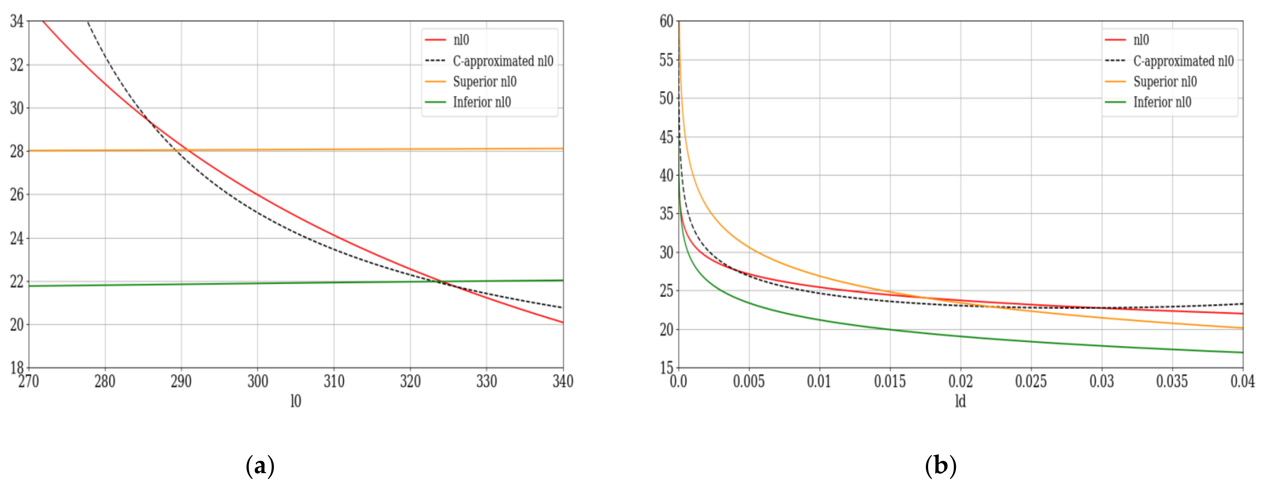
corresponds to the scale symmetry breaking. Attempting to explore other gauge types, a short revisit of the method used in our previous paper is in order; in that case, what was practically simplest possible gauge was picked:

$$\frac{\partial w}{\partial s}=Bw,$$

(7)

where the following notations are used:

$$F\left(x,\epsilon \right)\to w\left(s\right), s\equiv \ln \left(\frac{\epsilon }{{\epsilon }_0}\right).$$

(8)

It results that:

$$w\left(s\right) = w_0{e}^{Bs}.$$

(9)

Then, by replacing $\frac{\epsilon }{{\epsilon }_0}=a$, and choosing $B=-n\ln 2\ln a$ as our “staging parameter” of the given turbulent flow, where $n$ is the “stage number” of the turbulent cascade:

$$w_n\left(n\right) = w_0{a}^{-n\ln 2\ln a}.$$

(10)

Or computing and choosing the characteristic vortex scale as the given multifractal function, a stage-relative and scale-relative function are found through Equations (8–10):

$$l_n\left(n,s\right) = l_0{2}^{-n{s}^2}.$$

(11)

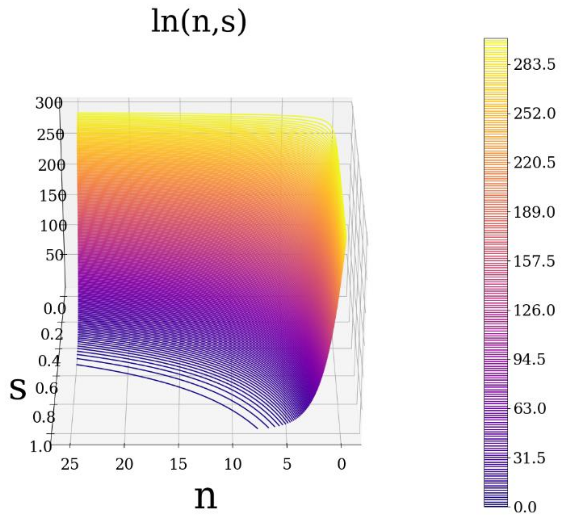
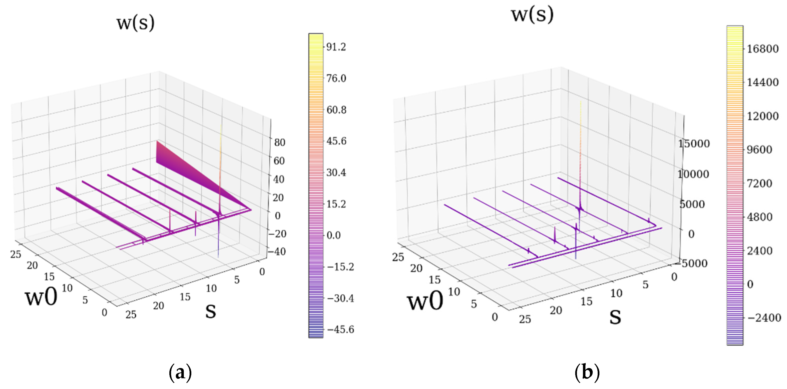
It is possible to observe that, through its dependency on scale resolution, $s$ practically determines how rapidly the scales of the turbulent cascade contract (Figure 1). The plot has been performed with $s$ values between $0$ and $1$, corresponding to a “slowed” contraction.

The following lateral plots show the dependency on $n$ and $s$ separately for a better representation of the function (Figure 2).

The main advantage of this model is its simplicity in formulation; despite a lack of complexity, this model has been shown to produce accurate and interesting results regarding atmospheric dynamics [14]. However, certain gauges present a much more variable behavior than the linear one used so far in our studies, and this variability can reveal more complex turbulent phenomena. It can be seen that, because of the manner of scale dependency contained in the scale evolution equation (Equation (11)), it is impossible for this gauge to lead to a model that predicts scale dilation—because the scale is squared, its sign becomes irrelevant and the exponent remains negative. Furthermore, the classic $\beta$ model is also incapable of simulating such behavior [15].

For more complex behavior, a Riccati-type gauge can be employed:

$$\frac{dw}{ds}-\frac{w^2}{M}+\frac{2R}{M}w-K=0$$

(12)

where $M$, $R$, and $K$ are other parameters that can be chosen to control staging. This equation can then be rewritten using the following notations:

$$M=2\mu , R=\pm c, KM=-d.$$

(13)

The result is:

$$2\mu \frac{dw}{ds}=w^2\pm 2c\mu -d.$$

(14)

This equation admits, with the restriction $d+c^2=-KM+R^2>0$, the following bounded solution:

$$s=-\frac{2\mu }{{\left(d+c^2\right)}^{\frac{1}{2}}}{\tanh }^{-1}\left[\frac{w\pm c}{{\left(d+c^2\right)}^{\frac{1}{2}}}\right]=-\frac{M}{{\left(-KM+R^2\right)}^{\frac{1}{2}}}{\tanh }^{-1}\left[\frac{w\pm R}{{\left(-KM+R^2\right)}^{\frac{1}{2}}}\right].$$

(15)

By setting:

$$A={\left(-KM+R^2\right)}^{\frac{1}{2}},$$

(16)

the following equation is obtained:

$$w\left(s\right) = c\pm A\tanh \left(\frac{As}{2\mu }\right) = R\pm {\left(-KM+R^2\right)}^{\frac{1}{2}}\tanh \left[\frac{{\left(-KM+R^2\right)}^{\frac{1}{2}}s}{M}\right].$$

(17)

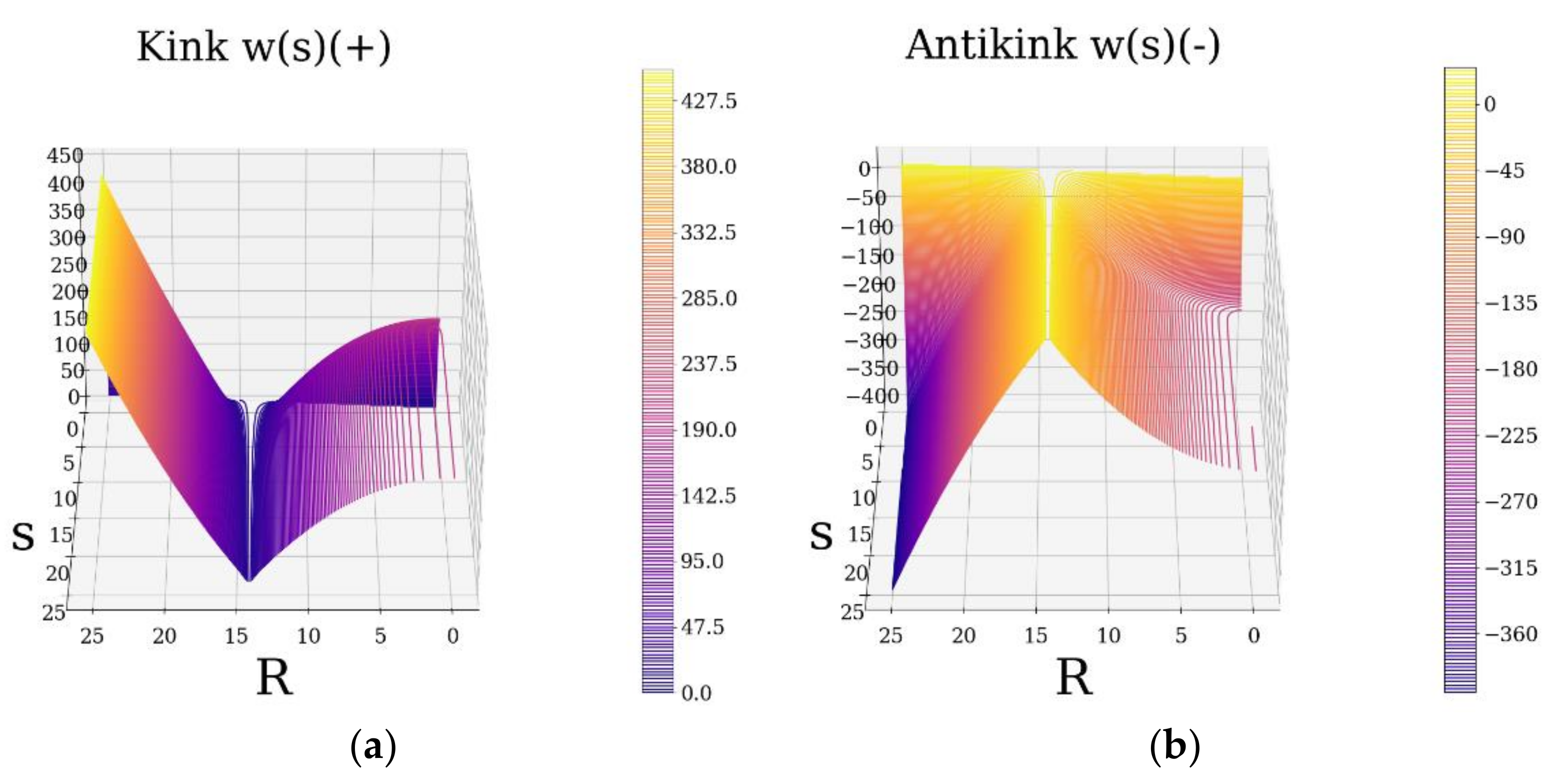
This equation can specify both multifractal kink-type $\left(+\right)$ as well as multifractal antikink-type $\left(-\right)$ behavior (Figure 3). The kink and antikink solutions found here describe two facets of the same problem. The simultaneous existence of both types of solutions clearly implies the possibility of both the scale dilation and contraction of our given multifractal function (Figure 3). $K$ acts as a type of “scrolling parameter” which increases or decreases the appearance of the phenomena which are about to be discussed; this parameter shall be valued $0$ when imposed and $1$ otherwise.

The kink-antikink equations present two types of evolutions depending on the parameter $M$: in the “left-handed regime” kink, $w$ progresses almost instantly throughout $s$ to an almost constant maximum value (Figure 4), meanwhile, for the “left-handed regime” antikink, the exact opposite happens. In the “right-handed regime”, the corresponding behavior of kink-antikink reverses and gains a smoothly-evolving (increasing or decreasing) characteristic across $s$ (Figure 4). It can be seen that the behavior most similar to that of the linear gauge is the right-handed kink if one considers $R$ to be connected to the staging; alternatively, the right-handed antikink can also be seen as similar if $R$ is considered to be connected to the inverse of the staging parameter (Figure 4). Multiple other instances of these diverse behaviors can be used to represent the turbulent energy cascade.

If, however, the Riccati-type differential equation, Equation (12), is rewritten using the notations:

$$M=-\frac{1}{f}, R=\frac{1}{2}, K=0,$$

(18)

it will form logistic equations of the multifractal type:

$$\frac{dw}{ds}=fw\left(1-w\right).$$

(19)

Its linearization by means of multiplication with $\frac{1}{w^2}$, in the following manner:

$$\frac{dn}{ds}=f\left(1-n\right), n=\frac{1}{w},$$

(20)

implies, by means of integration, the solution:

$$w\left(s\right) = \frac{1}{1-\left(1-\frac{1}{w_0}\right)exp\left[-f\left(s-s_0\right)\right]},$$

(21)

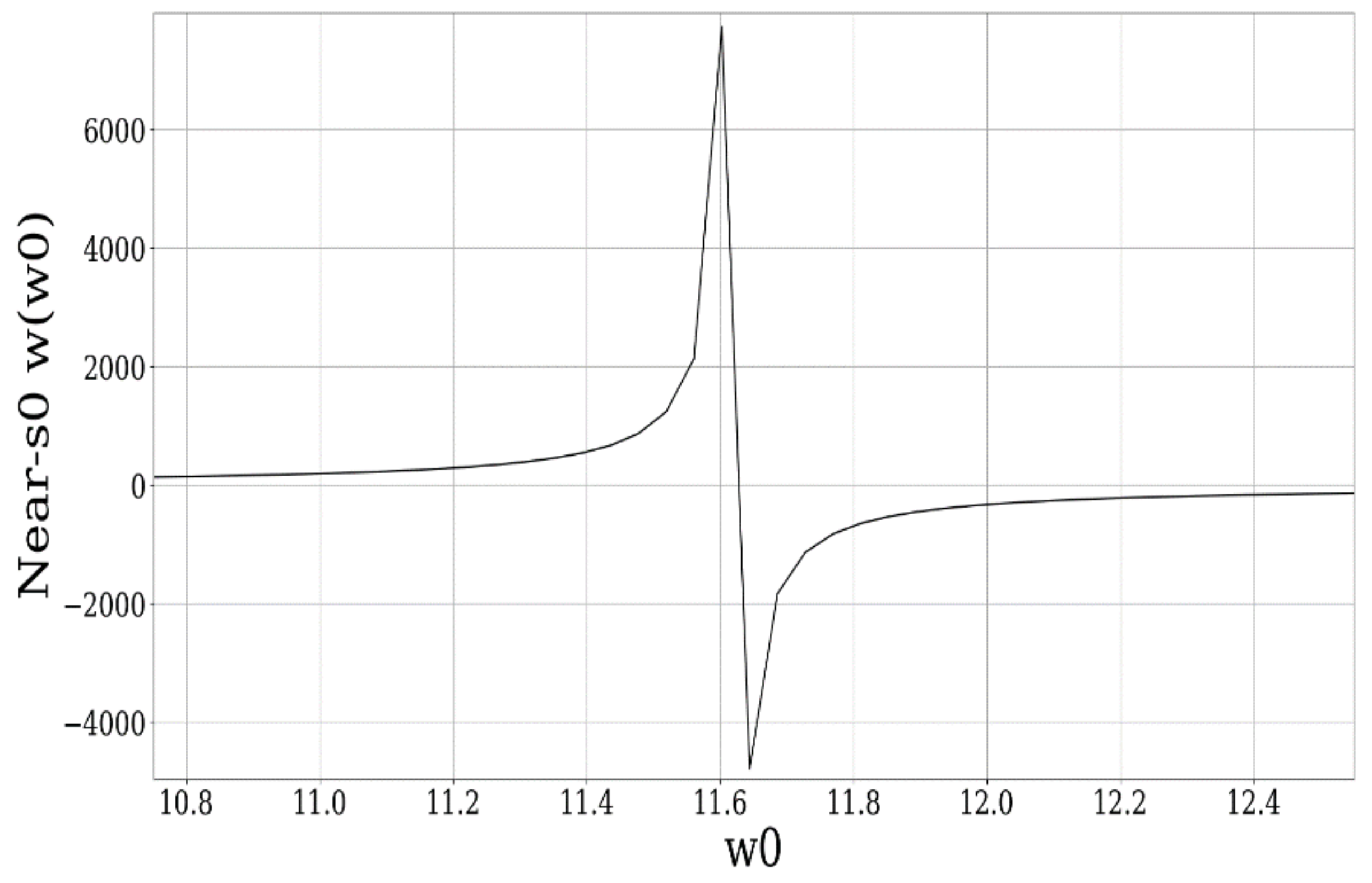
where $w_0$ and $s_0$ are two integration constants. The symmetry of the solution highlights the synchronicity of the two phenomena and the coupling between them—practically, the kink-antikink couple produces the maximum-minimum couple. This oscillating behavior occurs when $s$ is in the vicinity of $s_0$; this is seen in our figures by plotting the function with multiple chosen $s_0$. Important to note that this oscillation does not take place if $s$ is identical to $s_0$, because of the following identity:

$$w\left(s\right) = \frac{1}{1-\left(1-\frac{1}{w_0}\right)exp\left[-f\left(s_0-s_0\right)\right]}\equiv \frac{1}{1-\left(1-\frac{1}{w_0}\right)}\equiv w_0.$$

(22)

The following figure is an example of a peak in the vicinity of $s_0$ produced by the kink-antikink pairing (Figure 5).

Large $M$ values (of the order of hundreds) produce these left-right-hand regimes, but they correspond logically to very small $f$ values which show abnormal spikes in the other plot (Figure 6). Sub-unitary $M$ values yield reasonably-valued spikes, however, the left-right behavior found in (Figure 6) disappears. Overall, each instance of oscillating-like behavior in the vicinity of $s_0$ values can be treated as dilating or contracting cascades at various scale resolutions if $w_0$ is considered to be connected to the staging parameter $n$. In any case, the distributions of these kink-antikink spikes appear to be chaotic in nature, especially at high $M$ values.

The sheer richness of behavior exhibited by the Riccati gauge prove that it could be an excellent tool for developing models of various unstable, or otherwise turbulent, fluid flows; however, the main problem with issuing more complex gauges or gauging methods is the establishment of the presence of a staging parameter, $n$, which must obviously be an integer with values between $0$ and $n_{l_0}$. In the linear gauge used in our previous efforts, the positioning of this staging parameter was quite obvious. However, with the Riccati gauge, it is unclear which of the parameters of Equation (21), which is to say $f$, $w_0$, or $s_0$, might contain staging information. Because of this lack of clarity, it is also uncertain how one might use this gauge to construct a fully functional model using the constructor equations to determine turbulent energy per stage, fractal dimension per stage, and many other parameters (Equations (A10)–(A12)).

3. Connecting a Multifractal Turbulence $\mathit{\beta }$-Constant Model to the Logistic Map

For now, let us consider the conservation law of the specific impulse associated with the multifractal-nonmultifractal (see Equation (16) from [14]) under the specific form:

$$\left[{\partial }_t+V^l{\partial }_l+\left(\alpha +\beta \right){\partial }_l{\partial }^l\right]V^i=2\left(V_F^l{\partial }_l-\beta {\partial }_l{\partial }^l\right)V_F^i,$$

(23)

with:

$$V^i=V_D^i-V_F^i,$$

(24)

and:

$${\partial }_t=\frac{\partial }{{\partial }_t},{\partial }_l=\frac{\partial }{\partial X^l},{\partial }_l{\partial }^l=\frac{\partial }{\partial X^l}\frac{\partial }{\partial X^l},i,l=1,2,3.$$

(25)

In Equation (23) $t$ is the non-multifractal time with the role of the affine parameter of the motion curves, $X^l$ is the multifractal spatial coordinate, $V_D^i$ is the velocity field independent of scale resolutions, $V_F^i$ is the velocity field dependent on the scale resolutions, $V^i$ is the velocity field associated to the multifractal-non-multifractal transition, and $\alpha$, $\beta$ two constant coefficients associated to multifractal-non-multifractal transition with dependencies on scale resolutions (see Equation (9) from [14]).

Under a concrete form, imposed by the vectorial procedure, Equation (23) can be rewritten as:

$${\partial }_t\mathit{V}+\mathit{V}·\nabla \mathit{V}+\left(\alpha +\beta \right)∆\mathit{V}=\mathit{f},$$

(26)

where:

$$\mathit{f}=2\left({\mathit{V}}_{\mathit{F}}\nabla -\beta ∆\right){\mathit{V}}_{\mathit{F}}$$

(27)

is the specific multifractal force. Equation (26) is, in fact, a multifractal form of the Navier–Stokes equation. Now, introducing the normalized variables:

$$T=\frac{t}{t_0}, \mathit{U}=\frac{\mathit{V}}{{\mathit{V}}_{\mathit{0}}}, \mathit{R}=\frac{\mathit{r}}{{\mathit{r}}_{\mathit{0}}}, \mathit{F}=\frac{\mathit{f}{V}_0}{t_0}, r_0=V_0{t}_0,$$

(28)

where $t_0$ is the specific time, $V_0$ is the specific velocity, and $r_0$ is a specific length, the multifractal-type Reynolds number is found:

$$Re=-\frac{V_0{r}_0}{\alpha +\beta }, \alpha +\beta <0,$$

(29)

where we admit that $\alpha +\beta$ has the dimension $\frac{m^2}{s}$ according to Equation (26) to maintain $Re$ non-dimensionality.

Equation (26) then becomes:

$${\partial }_T\mathit{U}+\mathit{U}·\nabla \mathit{U}=R{e}^{-1}∆\mathit{U}+\mathit{F}.$$

(30)

coupled with the incompressibility equation:

$$\nabla ·\mathit{U}=0,$$

(31)

which together specify incompressibility at the multifractal-non-multifractal transition of the multifractal fluid.

We express the solutions in terms of the Fourier representation of $U$:

$$U\left(x,t\right) = {{\displaystyle \sum }}_k{a}_k\left(\tau \right)e^{ik·x}.$$

(32)

This resulting infinite system of ordinary differential equations of multifractal type for the Fourier coefficients is known as a Galerkin projection of multifractal type of the Navier–Stokes equations of the multifractal type:

$$\dot{a_i}=-{{\displaystyle \sum }}_{jk}{A}_{ilm}{a}_l{a}_m-\frac{a_i{\left|\mathit{k}\right|}^2}{Re}+F_i.$$

(33)

In this equation every mode $\dot{a_i}$ of multifractal type represents a component of the velocity field with a wave vector $\left|\mathit{k}\right|$ of the multifractal type. The velocity field at each length scale of multifractal type can be changed through nonlinear interactions of multifractal type with other modes through damping or forcing. The nonlinear interactions of multifractal types are quadratic and their strength is controlled by the coefficients $A_{ilm}$. Damping of multifractal type is inversely proportional to the wave vector of multifractal type and thus it is more efficient for small-scale modes of multifractal type. A detailed derivation of standard Equation (33) is given in [16]. Regarding potential issues with orthonormality, given the fact that the scaling resolution remains constant throughout an instance of the turbulent energy cascade (from the inner to the outer/dissipation scale), only differentiating various other types of energy cascades, and is therefore treated as a constant in the Fourier representation, the modes should remain orthonormal.

To simplify the problem let us remove all but a single arbitrary mode of multifractal type. This is a restriction of the standard Galerkin truncation, and it results in an equation of the form:

$$\dot{a}=-A{a}^2-\frac{a{\left|\mathit{k}\right|}^2}{Re},$$

(34)

i.e., an evolution equation of multifractal type for one mode forced by a quadratic nonlinearity and damping of multifractal types. A careful expansion of the Navier–Stokes equations of multifractal type would show that a mode of multifractal types cannot interact nonlinearly with itself. In other words:

$$A_{iii}=0.$$

(35)

However, we shall partially ignore this fact, since the obtained equation shows quadratic dissipation and nonlinearity of multifractal type, much like the Navier–Stokes equation of multifractal type. This makes it a useful tool, at least as an approximation. Here we will employ a simple forward Euler single-step explicit time integration procedure. This leads to:

$$\frac{a_{n+1}-a_n}{\tau }=-A{a}_n{}^2-\frac{a_n{\left|\mathit{k}\right|}^2}{Re}$$

(36)

where $\tau$ is an arbitrary discrete-time step parameter. We now rearrange Equation (36) as:

$$a_{n+1}=\tau A{a}_n\left(\frac{1-R{e}^{-1}\tau {\left|\mathit{k}\right|}^2}{\tau A}-a_n\right).$$

(37)

This multifractal map can be reduced to a well-studied example if we require that:

$$\frac{1-R{e}^{-1}\tau {\left|\mathit{k}\right|}^2}{\tau A}\equiv 1,$$

(38)

which implies that:

$$\tau A=1-R{e}^{-1}\tau {\left|\mathit{k}\right|}^2.$$

(39)

This in turn permits us to write Equation (37) as the following:

$$a_{n+1}=4\left(1-R{e}^{-1}\tau {\left|\mathit{k}\right|}^2\right)a_n\left(1-a_n\right) =r{a}_n\left(1-a_n\right),$$

(40)

which is a logistic map of the multifractal type. While the novelty of this development can be found in its multifractality and the following applications, other studies have been written which draw an equivalence between the logistic map and the Navier-Stokes equations [17,18]. It is easily seen that as $Re\to \infty$, $r\to 4$. Since $a_n\left(1-a_n\right)$ has a maximum at $\frac{1}{4}$ for $a \in \left[0,1\right]$ we see that we must rescale $r$ by a factor of $4$ to obtain a range of values for $r$ that is between $0$ and $4$, just like in the case of the logistic map. It is also worth observing that $r$ depends on $\left|\mathit{k}\right|$ and on the time step parameter. In particular, we see that the product of these factors must be less than $Re$ for $r>0$ to hold.

Now, the parameters contained in $r$ must be identified; it is quite obvious that $Re$ is Reynolds’ number. Meanwhile, $\tau$ shall be the period of the dynamical system described by the logistic map. The interpretation of the arbitrary wave vector $\mathit{k}$ can be quite debatable, but we shall assume it, for now, to be equal to a standard interpretation $\left|\mathit{k}\right| = \frac{1}{l_n}$. However, certain theoretical considerations could yield a different interpretation. The length scales produced by $l_n$ decrease in size, from supra-unitary to sub-unitary measures—if the standard interpretation of the wave vector is used, it is found that $r$ will evolve from $4$ to $1$ if $\tau =ct.$, which is exactly the opposite of what the model should produce. According to the typical bifurcation sequence for the Navier-Stokes equations given by Ruelle and Takens, which is $steady\to periodic\to quasiperiodic\to chaotic$, it is unrealistic for the turbulent flow to be modeled such that $r=4$ corresponds to the largest scales [19]. It must be highlighted that this standard route to chaos is also followed by the logistic map. It stands to reason that the elements contained in $r$ decrease instead of increase, so that the term $R{e}^{-1}\tau {\left|\mathit{k}\right|}^2$ ends up decreasing in time, and $4\left(1-R{e}^{-1}\tau {\left|\mathit{k}\right|}^2\right)$ ends up increasing. This is fixed by the variability of $\tau$, as the temporal scale employed here must be period doubling.

To calculate $\tau \left(n\right)$, we consider a set of equations found in our previous work; more specifically, we consider Equation (14) and the equations leading up to it [14]. It is necessary for $\tau \left(n\right)$ to be represented by a counterpart equation to the $l_n\left(n\right)$ found in Equation (14)—however, this counterpart must be increasing and steadily doubling. The following formula is used:

$$\tau \left(n\right) =\frac{{\left(2t_0\right)}^n}{t_0{}^{\left(n-1\right)}}.$$

(41)

where $t_0$ is the period of the initial vortex, and it is found through Equation (14) of our previous work as $t_0=\frac{l_d\sqrt{Re}}{u_d}$. The non-dimensionality of $U$ in the equation used to initialize this demonstration solves any issues regarding the dimensionality of the logistic map parameter $r$; because the parameters of the non-dimensional function $U\left(x,t\right)$ are also non-dimensional, the wave vector itself shall exhibit non-dimensionality.

For the following approximation, Reynolds’ number shall also be considered through the popular approximation $Re={\left(\frac{l_0}{l_d}\right)}^{\frac{4}{3}}$.

Compiling these conclusions yields:

$$a_{i+1}=4\left[1-\frac{\tau \left(n\right)l_d{}^{\frac{4}{3}}}{l_n{\left(n\right)}^2{l}_0{}^{\frac{4}{3}}}\right]a_i\left(1-a_i\right).$$

(42)

Now, it is expected that, if the logistic map were a perfect fit for the behavior of the nondimensional equation that we started with, the term $4\left[1-ℂl_n{\left(n\right)}^2\right]$ would produce values that match the $r$-values at which a bifurcation takes place in the bifurcation diagram of the logistic map. These values are

$$L_{1,2,3,4,\dots }=\left\{1,3,1+\sqrt{6}, 3.54409,\dots \right\}.$$

(43)

Thus, we expect:

$$4\left[1-\frac{\tau \left(\left\{0,1,2,3,\dots \right\}\right)l_d{}^{\frac{4}{3}}}{l_n{\left(\left\{0,1,2,3,\dots \right\}\right)}^2{l}_0{}^{\frac{4}{3}}}\right]=L_{1,2,3,4,\dots }.$$

(44)

Now, supposing that $\tau$ is in fact constant, let $l_0=300m$ as a basic example. Replacing it in the afferent equation so that $r=3$ it is seen that $l_1=100\sqrt{3}m$ is required, thus $\frac{l_0}{l_1}=\sqrt{3}$. Continuing, $l_2=100\sqrt{9-3\sqrt{6}}m$ is obtained, however, this yields $\frac{l_1}{l_2}=\sqrt{\frac{3}{9-3\sqrt{6}}}$. The fact that $\frac{l_0}{l_1}\ne \frac{l_1}{l_2}$ implies that, for the model to compute parameter values that correspond to bifurcations at every turbulent cascade stage change, $\beta$ cannot be constant—this contradicts our model which presupposes a constant $\beta$ from the very beginning. Indeed, even attempting to implement the classic $\beta$ model, we obtain:

$$a_{i+1}=4\left[1-\frac{\tau \left(n\right)l_d{}^{\frac{4}{3}}}{l_0{}^{\frac{10}{3}}{2}^{-2n}}\right]a_i\left(1-a_i\right),$$

(45)

which, besides not even considering any modifications to the variability of the period, does not yield bifurcation-matching results.

Moving on, it is expectable that this modified logistic map would follow a Feigenbaum-type theorem in some manner; all one-dimensional maps with a single quadratic maximum are supposed to present bifurcation parameters according to the following rate [20]:

$$\frac{r_{n-1}-r_{n-2}}{r_n-r_{n-1}}\cong \phi .$$

(46)

Given the fact that the staging implemented in the parameter $r$ acts as a kind of “forcing” for the positioning of a bifurcation in the $r$-space of our modified logistic map, it should be expected that the relationship will also produce a constant, yet one which will not necessarily be Feigenbaum’s constant, $\delta =4.6692$. Indeed, using the previously-found description of $r$ it is possible to obtain:

$$\frac{{\tau }_{n-2}{l}_{n-1}{}^2{l}_n{}^2-{\tau }_{n-1}{l}_{n-2}{}^2{l}_n{}^2}{{\tau }_{n-1}{l}_{n-2}{}^2{l}_n{}^2-{\tau }_n{l}_{n-2}{}^2{l}_{n-1}{}^2}\cong \phi .$$

(47)

It is possible that this relation would produce a constant; however, this constant appears to be valid for the given initial parameters of the model—thus, for a single given instance of a turbulent energy cascade.

Overall, the differences between the basic logistic map and the $\beta$ model can be deceptive; for example, the classic $\beta$ model is exactly scale-halving, but this does not necessarily mean that the logistic map, which presents period-doubling behavior, will match in terms of specific bifurcation parameters. It bears reminding that the connection between the logistic map and the equations governing the velocity field is approximate, and a $\beta$-constant model is an approximation on its own. In any case, this connection can be used to approximate whether or not, for a given turbulent cascade, certain stages of it present “non-chaotic” or otherwise laminar or semi-laminar behavior. Various turbulent regimes and their potential for chaos can be identified in this manner—this possibility has more to do with the nature of the bifurcation diagram of the classical logistic map. 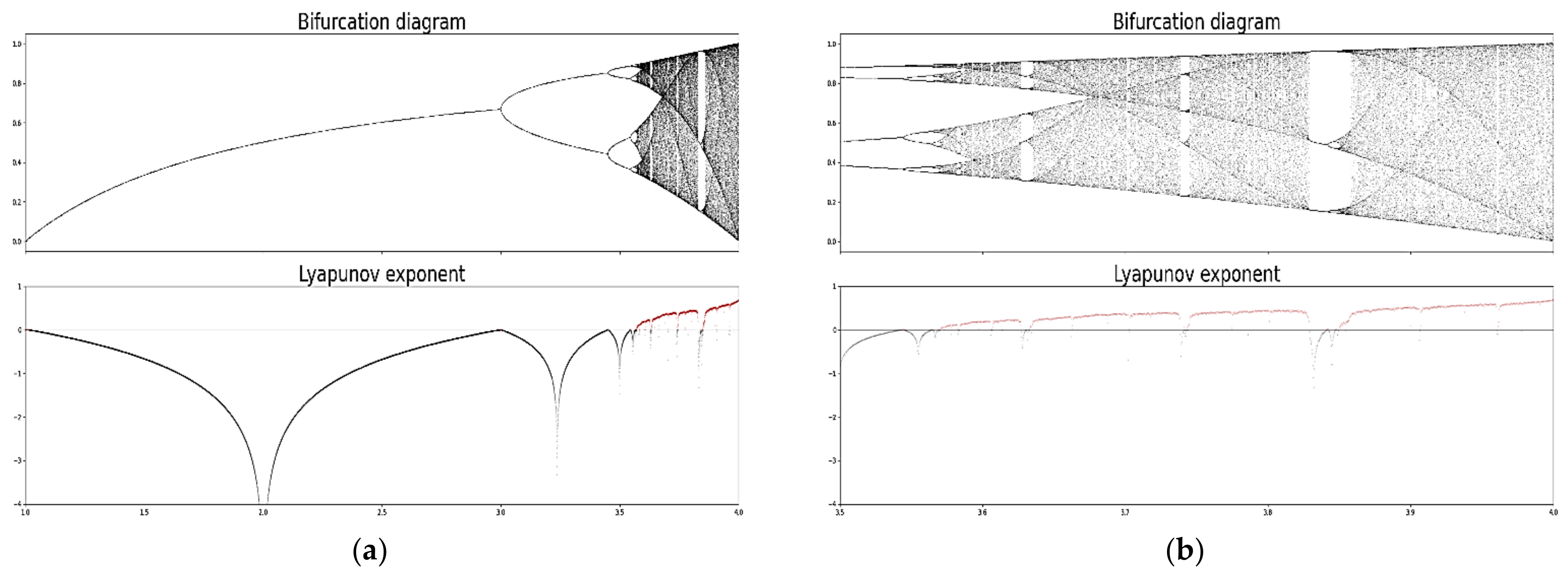More specifically, there exists a segment in this bifurcation diagram, approximately between $3.56995$ and $3.82843$ in terms of $r$ values, which is commonly named the “Pomeau-Manneville scenario”, which is characterized by various instances, or “islands”, of laminar or otherwise non-chaotic behavior (Figure 7) [21]. For certain initial values, and at certain scales and periods, it is then possible to arrive at such $r$ values characterizing laminar regions, which would imply that, at certain scales and altitudes, atmospheric flow can spontaneously exhibit laminar behavior.

For example, let us consider the quite-obvious three main stability intervals in the chaotic section of the bifurcation diagram:

$$3.83\le 4\left[1-\frac{\tau \left(n\right)l_d{}^{\frac{4}{3}}}{l_0{}^{\frac{10}{3}}{2}^{-2n}}\right]\le 3.855,$$

(48)

$$3.74\le 4\left[1-\frac{\tau \left(n\right)l_d{}^{\frac{4}{3}}}{l_0{}^{\frac{10}{3}}{2}^{-2n}}\right]\le 3.742,$$

(49)

$$3.627\le 4\left[1-\frac{\tau \left(n\right)l_d{}^{\frac{4}{3}}}{l_0{}^{\frac{10}{3}}{2}^{-2n}}\right]\le 3.632.$$

(50)

It can be seen that one of them is not, strictly speaking, in the Pomeau-Manneville region, yet it is still a region of negative-Lyapunov exponent (Figure 7). To more accurately determine whether or not these inequalities can be satisfied in a given case, it is imposed that for the given initial parameters laminar, periodic, or otherwise non-chaotic behavior is found at an $n$ scale if there exists a positive integer $n$ in the previous inequalities, once they are expanded. Of course, there exist other smaller non-chaotic intervals as well, for which other such inequalities could be constructed.

4. Results and Discussions

In the following segment of this paper, experimental data obtained via a lidar platform is introduced to apply the theory and verify the results. The finer details of the method used to obtain the following data profiles, named the “Roșu-Tatarski method”, are described in greater detail in our previous works, however, they rely on obtaining the structure coefficient of the refraction index profile $C_N^{2 }\left(z\right)$ in the following manner [14,22]:

$${\sigma }_I^2\left(L\right) =1.23 C_N^{2 }\left(L\right)k^{\frac{7}{6}}{L}^{\frac{11}{6}}.$$

(51)

With ${\sigma }_I^2\left(L\right)$ being the “scintillation” (or, in this case, the logarithm of the standard deviation of light intensity) of a source of light observed from a distance represented by the optical path $L.$ The definition:

$${\sigma }_I^2\left(L\right) =\ln \left(1+\frac{\langle I{\left(L\right)}^2\rangle -\langle I{\left(L\right)\rangle }^2}{\langle I{\left(L\right)\rangle }^2}\right).$$

(52)

Is given, with $I\left(L\right)$ being the intensity of the range-corrected signal at the particular point in the optical path, which is analogous with the $RCS$ intensity. Having determined the $C_N^{2 }\left(z\right)$ profile, it is now possible to calculate, with a degree of approximation, the length scales. The inner scale profile is linked to scintillation:

$${\sigma }_I^2\left(L\right) \cong 0.615 C_N^{2 }\left(L\right)L^3{l}_d{\left(L\right)}^{\frac{-7}{3}}.$$

(53)

While the outer scale is linked to the $C_N^{2 }\left(z\right)$ profile:

$$C_N^2\left(z\right) = l_0{\left(z\right)}^{\frac{4}{3}}{\left(\nabla \langle n\left(z\right)\rangle \right)}^2.$$

(54)

With turbulent eddies within the inertial subrange, the refraction index profile can be approximated from the definition of the respective structure coefficient:

$$n\left(z\right) \cong n_0-\sqrt{C_N^2\left(z\right)z^{\frac{2}{3}}}.$$

(55)

Which then gives us the means to extract the outer scale profile.

This method is well-referenced in our studies and has been already used successfully multiple times. Once the outer and inner/dissipation scales have been obtained, the modified beta model developed in our latest work can be employed to obtain the rest of the turbulent parameters considered in this manuscript. It is of interest to check if the various profiles yielded through theory in this study present realistic values in both evolution and order; added upon the qualitative nature of this comparison, results pertaining to the degree of chaos exhibited by the atmosphere are obtained.

The experimental data used to solve these equations is calculated by analyzing lidar RCS (Range Corrected Signal) data obtained from the lidar platform at the Optical Atmosphere Spectroscopy and Lasers Laboratory, part of the Faculty of Physics in the “Alexandru Ioan Cuza” University, at the coordinates 47.19306° North and 27.55556° East. The methodology used in producing the initial and dissipation scale profiles is reliant on calculating the scintillation profiles of the lidar signal by observing the variation between multiple RCS profiles, which is then used to produce the coefficient of the structure-function of the atmospheric refractive index $C_N^{2 }$ [22]. This is then employed to construct a timeseries of $\langle \epsilon \rangle$, $n_{l_0}$, and $\langle D_F\left(n\right)\rangle$.

The technical specifications of the main components of the lidar platform used in our study are an Nd:YAG laser component producing laser pulses at a frequency of $30\mathrm{Hz}$, with a wavelength of $532\mathrm{nm}$, the laser beam diameter of $6$ mm, and a pulse energy of $100\mathrm{mJ}$ and a Newtonian LightBridge telescope with a primary mirror diameter of $406\mathrm{mm}$. The lidar platform utilized in the study has a spatial resolution of $3.75\mathrm{m}$ and both technical details and results from previous measurement campaigns were reported in the scientific literature in independent studies [23,24] and in our previous studies [13,14,22,24]. The profile is calculated by software written in Python 3.6 [22]. The signal overlap altitude in all cases is much lower than the PBLH. Profiling with two different temporal resolutions were performed, $15\mathrm{s}$ and $10$ s, respectively—there is evidence to suggest that a lower temperature profile yields more accurate results with the given method, because its validity relies on the approximation that the total amount of parameter inhomogeneity (which, in this case, is the atmospheric refraction index) in the atmospheric column is constant, which is only true for small intervals of time [22].

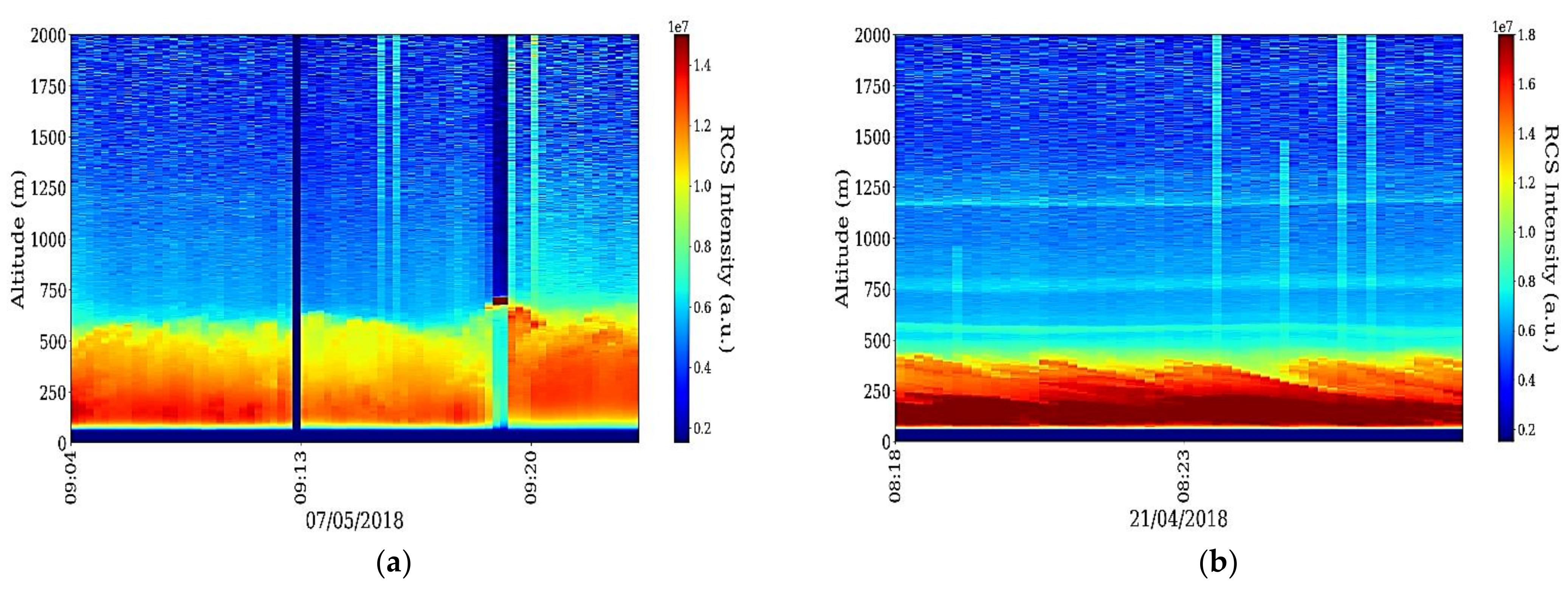
The improvements brought to the model now allow us to avoid the approximation of $l_1\left(z\right) \cong \frac{2}{3}{l}_0\left(z\right)$, which was used in our previous study, by using only the parameters $l_0$ and $l_d$ to initialize our model with Equation (A17) Appendix A. The following figure is a timeseries of the RCS lidar signal used to calculate the length scales according to the presented theory (Figure 8); this figure is presented to ascertain with accuracy the location of the PBL (Planetary Boundary Layer) relative to values obtained in the rest of the timeseries.

The timeseries associated with $C_N^{2 }$ are shown next (Figure 9); beyond any further uses in the associated calculations, this coefficient is associated with optical turbulence strength, and thus with turbulence intensity in general [25]. A more detailed investigation of potentially anomalous values of $C_N^{2 }$ must be performed next; the Fried parameter is inversely proportional to the integral of $C_N^2\left(z\right)dz$, however, it is also proportional to the wavelength in the following manner [26,27]:

$$r_0={\left(\frac{0.06{\lambda }^2}{{{\displaystyle \int }}_0^{2000}{C}_N^2\left(z\right)dz}\right)}^{\frac{3}{5}}.$$

(56)

The integration limits have been chosen according to the relevant shown profile. It is found that $C_N^2$ values are slightly overestimated at higher altitudes, at least compared with values found in other studies [28,29]. However this is due to a loss of useful signal: practically, in the context of our data collection, we have used a shortened acquisition time (resulting in profiles every $10 \mathrm{s}$ or $15 \mathrm{s}$) which means that the actual “useful signal” profile range has decreased. For the typical 1 min profiling regime used for this platform, the useful signal range is approximately $6–7 \mathrm{km}$. However, for this shortened acquisition time, the range has decreased to approximately $2 \mathrm{km}$. This means that data obtained at, or slightly under, $2 \mathrm{km}$ is somewhat unreliable. At the same time, one must consider the lidar overlap distance, in which data can also be considered to have a degree of unreliability. Changing the integral limits so that $0$ is replaced by $300$ and $2000$ is replaced by $1700$, it is found that ${{\displaystyle \int }}_{300}^{1700}{C}_N^2\left(z\right)dz \cong {10}^{-11}$ for most of the profiles in the timeseries. Given that the working wavelength of the lidar is $532 \mathrm{nm}$, it is found that $r_0\cong 2 \mathrm{cm}$, again, for most of the profiles in the timeseries, which is a rather normal value.

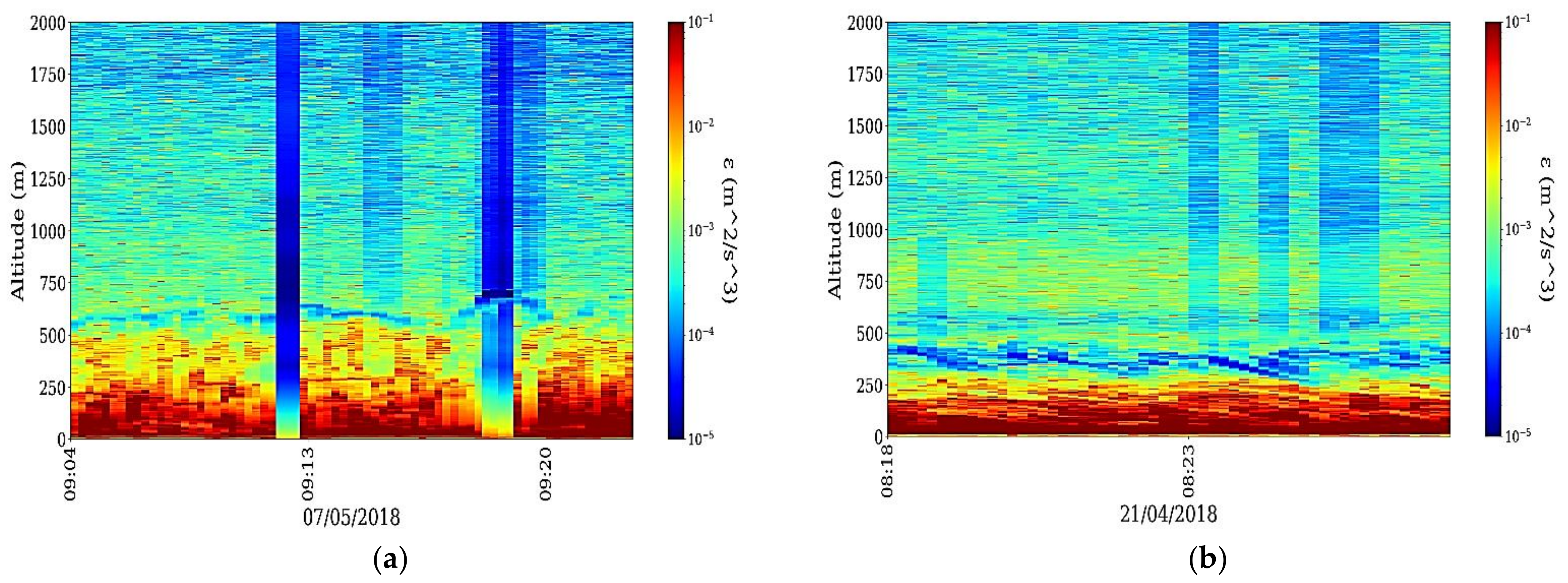
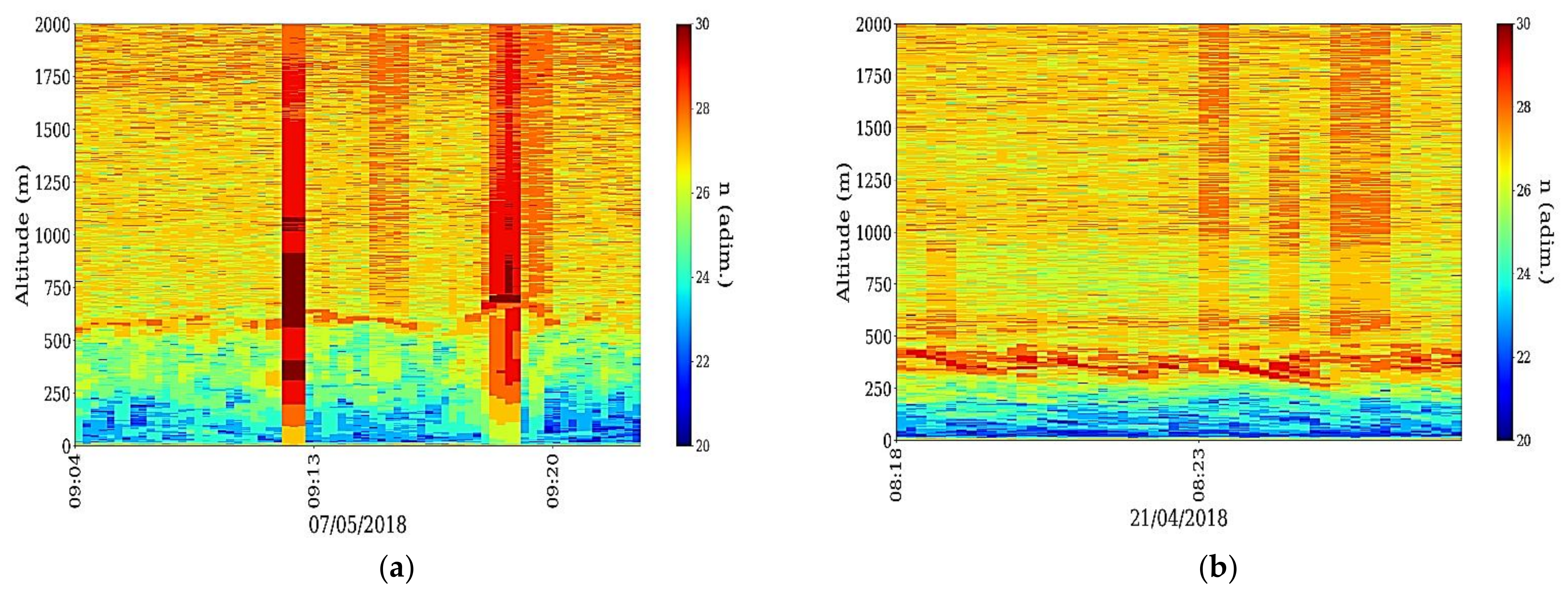
Observing the next timeseries, $\langle \epsilon \rangle$ values seem to be at their lowest in or near the region of the PBL (Figure 10); multiple studies seem to support the fact that turbulent dissipation is lowest at, or just above, the PBL, with both experimental and theoretical data [30,31].

The altitude variability of $n_{l_0}$ shown by the timeseries does not appear to be high, roughly between $20$ and $30$ (Figure 11), but a higher variability should not be expected given relatively low values. It must be highlighted that $n_{l_0}$ values seem to be highest in the PBL region, with dissipation values seeming to be at their lowest. It has been determined that a lower dissipation means that the energy cascade requires more stages to manifest itself from $l_0$ to $l_d$ [13,14]; the implication is that atmospheric PBL turbulent behavior is much more long-lived and more “resilient” to turbulent energy dissipation, which does indeed justify why this layer is such a stable and easily-recognizable feature of the atmosphere in most meteorological scenarios.

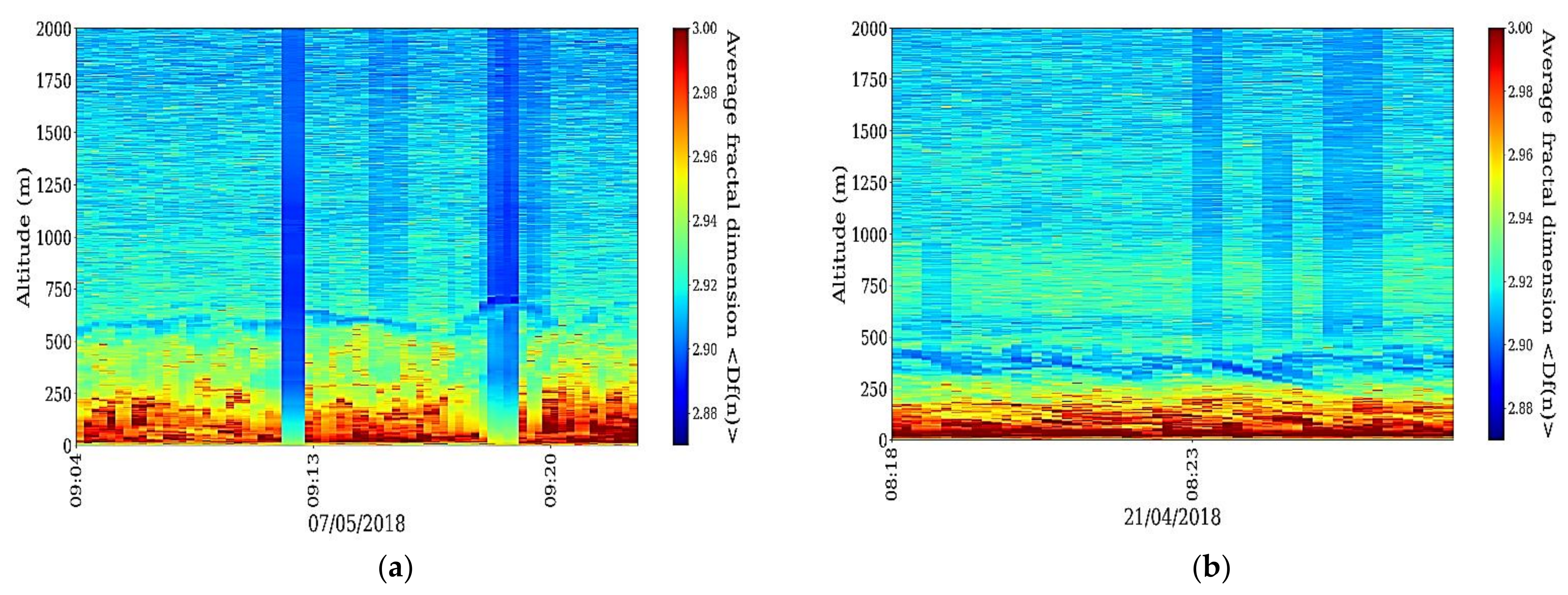
With the timeseries composed of $\langle D_F\left(n\right)\rangle$, it is possible to qualitatively determine a degree of atmospheric multifractality and atmospheric turbulent evolution; it can be seen that regions associated with the PBL exhibit a smaller $\langle D_F\left(n\right)\rangle$ and thus larger scales and a potentially less-developed (or longer-lasting) turbulent regime (Figure 12). This is in concordance with dissipation values being smaller in the region of the PBL—one would expect that less dissipation implies a more resilient turbulent energy cascade wherein the larger, less convoluted scales “survive” longer before bifurcation (Figure 12).

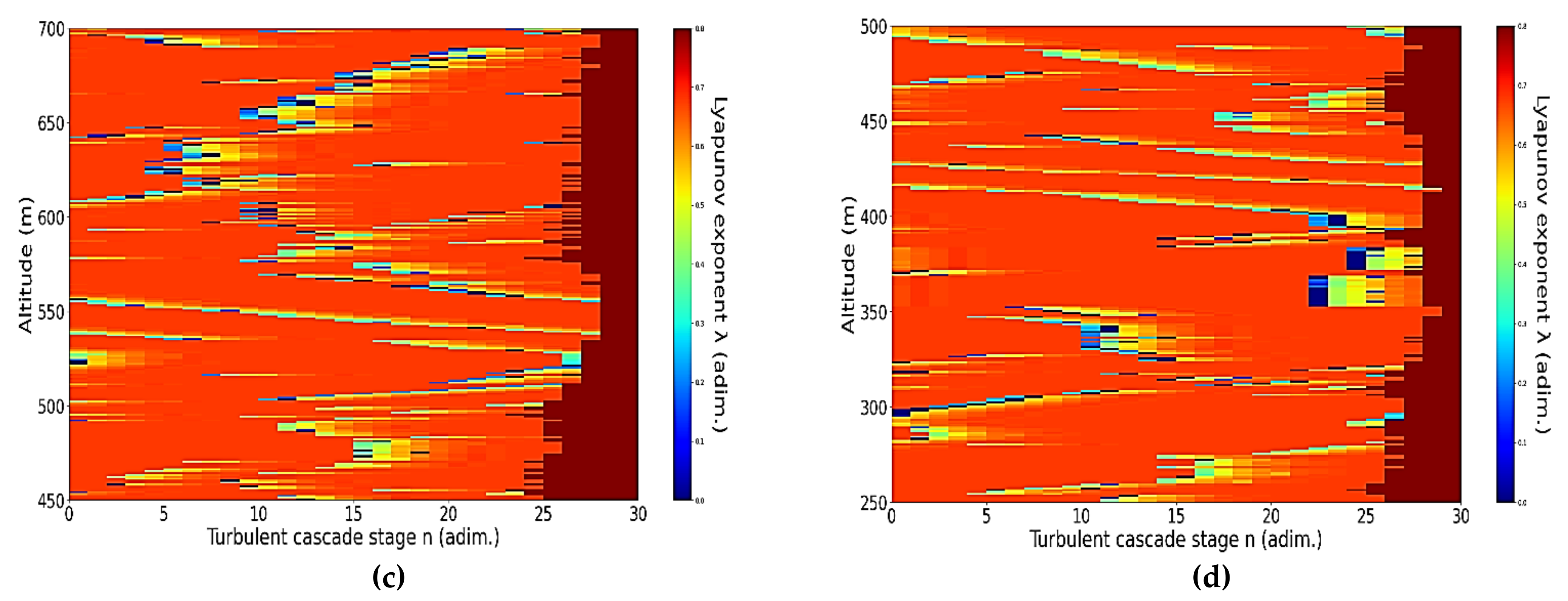
An analysis of the chaotic behavior of the turbulent cascade in an atmospheric profile is then performed in the following manner: calculating $l_n\left(n\right)$ for each altitude throughout the possible stages, a number of $r$ values are naturally obtained, and these are then used to calculate corresponding maximal Lyapunov exponents. These exponents are then used to quantify the “chaoticity” of the given stage of the turbulent cascade at a given altitude, aided by the colormap plot (Figure 13). It is noticed that a maximal number of stages is reached at a certain point; according to results from our recent studies, this area is indicative of the position of the PBLH [13,14]. And, indeed, there exist distinct regions of horizontal laminarity at relatively large scales right where the PBLH is supposed to be manifested (Figure 13). It appears that above the region roughly indicating the PBLH, the occurrence frequency of these non-chaotic intervals becomes more or less constant; the density of these semi-laminar events may remain the same throughout much of the lower free atmosphere.

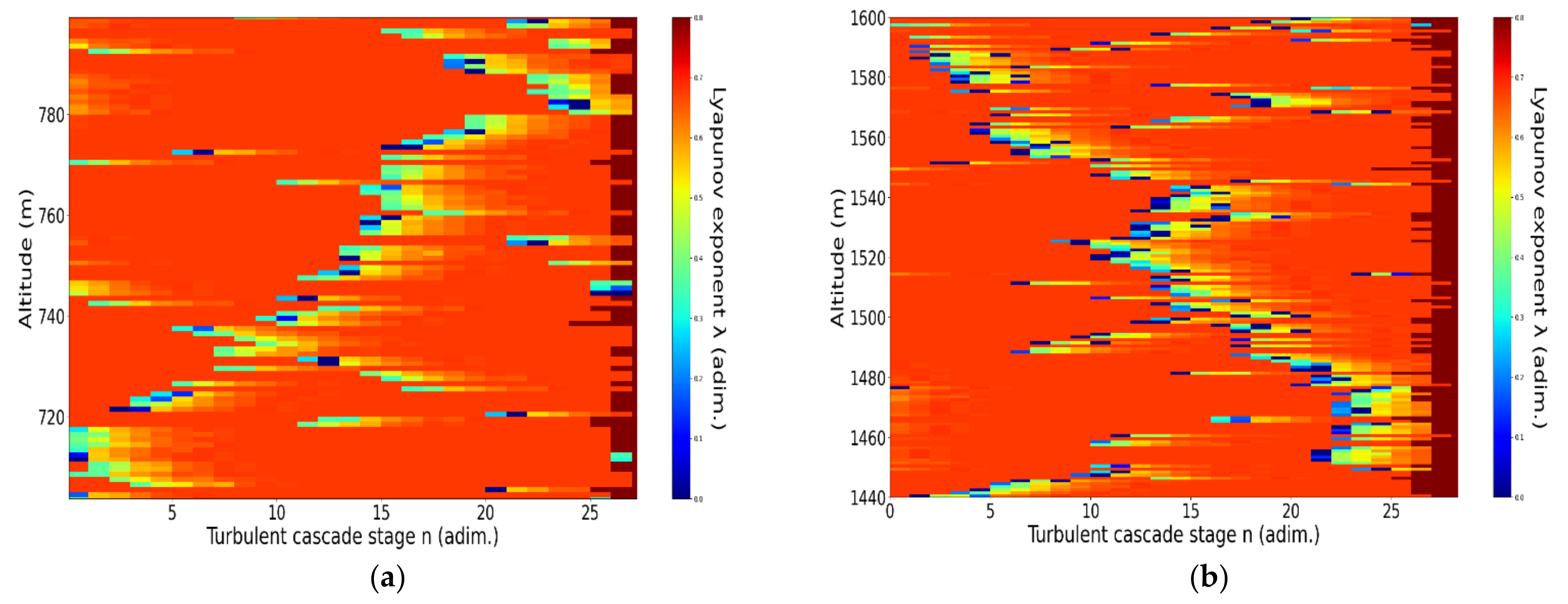
It is also possible to observe what appear at a first glance to be “V-shaped structures”; these slopes shall be named “laminar channels”, and their appearance is a natural consequence of the fact that, at a certain altitude, the inequality necessary for laminar behavior is satisfied, and then satisfied again at a different altitude at a different or similar scale (Figure 14). We thus identify “ascending” or “descending” laminar channels, and these structures can help explain various atmospheric transport phenomena regarding aerosols and cloud formations, but also regarding PBL stability.

It is difficult to determine, with both ascending and descending laminar channels, whether or not their direction has any connection to a potential transport phenomenon upwards or downwards; however, given the fact that the cascade proceeds naturally towards the dissipation scale, it is perhaps safe to assume that an ascending channel (which shows progress across staging at an increase in altitude) would represent upwards transport phenomena and that a descending channel (which shows progress across staging at a decrease in altitude) would represent downwards transport phenomena (Figure 14). Finally, in general, for all obtained timeseries, the horizontal stripes of either very high or very low values are produced due to signal noise present in the RCS lidar data used to calculate the length scales.

5. Conclusions

In this paper the non-linear behavior and functionality of the atmosphere have been assimilated under a multifractal approach, applying scale resolution and scale symmetry breaking theories. These theories can aid in the formulation of gauges for multifractal functions of atmospheric parameters, which can then be interpreted as evolution equations for the given parameter in the staging of the turbulent energy cascade. The case of a Riccati gauge is considered, which is an example of a more complex gauge that has the potential of simulating and illustrating interesting and complex turbulent behavior—however, this behavioral richness is contrasted to the difficulty in properly parameterizing it in connection to the turbulent staging. Next, to overcome these difficulties, it is shown that a simpler model constructed through a linear gauge can be connected to a modified form of the logistic map, which approximates under certain conditions the multifractal equations of motion of a turbulent atmospheric multifractal flow. The introduction of this model in the logistic map implies an associated Lyapunov exponent for each of the turbulent objects with length scales corresponding to the model staging—in this manner, it is possible to determine whether or not, for a given set of initial parameters and at a given altitude in an atmospheric column, there exist stages in the turbulent cascade that present momentary laminar qualities.

In the derived equation system, from an atmospheric modeling and forecast point of view, the initial quantities are the injection and dissipation scales themselves; but these quantities can be obtained as an atmospheric profile through a method detailed in one of our previous studies with a lidar platform. Employing these profiles, timeseries of some of the various parameters detailed in this study have been compiled, and it has been found that, especially regarding the known behavior of the PBL, they are in accord with the presented theory and existing scientific literature. Furthermore, laminar channels are indeed found in the given atmospheric columns—these are ascending or descending in terms of their relation to altitude and turbulent cascade stage, and they can be the source of various types of transport phenomena. In fact, it is found that the region of the PBL is represented, in both cases, by horizontal strongly-non-chaotic regions at large scales. From a prospective perspective, a future study might include a more detailed analysis of the predictability of atmospheric transport phenomena connected to these laminar channels; it would also be possible and productive to construct hierarchies of gauges and quantify their usability. Finally, progress could be made towards a model which is not necessarily $\beta$-constant, which might exhibit staging that matches perfectly to the bifurcation points of the logistic map—such a model might be constructed and studied similarly to the procedures contained in this study.