Article

Towards a Real-Time Description of the Ionosphere: A Comparison between International Reference Ionosphere (IRI) and IRI Real-Time Assimilative Mapping (IRTAM) Models

Istituto Nazionale di Geofisica e Vulcanologia, Via di Vigna Murata 605, 00143 Rome, Italy
*
Author to whom correspondence should be addressed.
Atmosphere 2021, 12(8), 1003; https://doi.org/10.3390/atmos12081003
Submission received: 9 July 2021 / Revised: 30 July 2021 / Accepted: 1 August 2021 / Published: 4 August 2021
(This article belongs to the Special Issue Ionospheric Monitoring and Modelling for Space Weather)

Abstract

:
This paper focuses on a detailed comparison, based on the F2-layer peak characteristics foF2 and hmF2, between the International Reference Ionosphere (IRI), which is a climatological empirical model of the terrestrial ionosphere, and the IRI Real-Time Assimilative Mapping (IRTAM) procedure, which is a real-time version of IRI based on data assimilation from a global network of ionosondes. To perform such a comparison, two different kinds of datasets have been considered: (1) foF2 and hmF2 as recorded by 40 ground-based ionosondes spread all over the world from 2000 to 2019; (2) foF2 and hmF2 from space-based COSMIC/FORMOSAT-3 radio occultation measurements recorded from 2006 to 2018. The aim of the paper is to understand whether and how much IRTAM improves IRI foF2 and hmF2 outputs for different locations and under different diurnal, seasonal, solar and magnetic activity conditions. The main outcomes of the study are: (1) when ionosonde observations are considered for validation, IRTAM significantly improves the IRI foF2 modeling both in accuracy and precision, while a slight improvement in the IRI hmF2 modeling is observed for specific locations and conditions; (2) when COSMIC observations are considered for validation, no noticeable improvement is observed from the IRTAM side for both foF2 and hmF2. Indeed, IRTAM can improve the IRI foF2 description only nearby the assimilated ionosonde locations, while the IRI hmF2 description is always more accurate and precise than IRTAM one.

1. Introduction

Space Weather events can have a deep negative impact on the technological systems, such as power systems, satellites, Global Positioning System (GPS), pipelines, and communication cables. The damages suffered by these systems, on which our society is nowadays greatly dependent, besides leading to very high costs, can also significantly affect human life [1,2]. Therefore, in this context, in recent years the near real-time specification of the ionosphere has become more and more important to nowcast and possibly mitigate the adverse consequences of Space Weather events. For this purpose, several models able to assimilate real-time ionospheric measurements have been recently proposed [3,4,5,6,7,8,9,10,11,12,13,14,15,16].
Some climatological models already existent were adapted for the quasi real-time assimilation of ionospheric data. One outstanding example is the IRI-based Real-Time Assimilative Model (IRTAM) [17,18] that, by ingesting ionosonde-derived F2-layer peak parameters values, updates the underlying empirical global climatological knowledge of the ionosphere provided by the International Reference Ionosphere (IRI) model [19,20], thus supplying a global real-time representation of the ionosphere. The assimilation of real-time measurements in a background empirical model is one of the most applied and fruitful methodologies for the real-time specification of the ionospheric electron density. In this context, the knowledge of the large-scale climatological behavior of the ionosphere provided by the underlying background empirical model is complemented with the small-scale weather information provided by real-time assimilated data. The effectiveness and quality of such data-assimilation procedures is critically dependent on the applied algorithm, on the quality, spatial distribution, and availability of assimilated data, and of course on the underlying background empirical model.
Empirical models, such as IRI, are based on analytical formulations whose numerical coefficients are obtained on the basis of the underlying datasets; as a consequence, when new datasets are released, it is of utmost importance to validate the model against new data and eventually recalculate the model’s coefficients with the inclusion of the newest data. This validation and recalculation scheme is an ongoing process for empirical models and leads to the continuous improvement of the model itself. Over the years, IRI underwent many validation studies and comparisons with other ionospheric models [21,22,23,24,25,26,27,28]; on the contrary, validations of the IRTAM model are restricted to the works by Vesnin [29] and Galkin et al. [18] for specific locations and conditions. Due to the ever-growing importance that IRTAM is gaining as the most used and affirmed real-time specification of the ionosphere, it is important to validate its performances against large and different datasets to quantify the improvement made by IRTAM in the description of ionospheric weather when compared to the climatological representation made by IRI.
In the present paper, a global validation of the ionosphere F2-layer peak characteristics as modeled by IRI and IRTAM is presented. Specifically, the IRI and IRTAM models, the latter assimilating both the F2-layer ordinary critical frequency (foF2) and the F2-layer peak height (hmF2) from ground-based ionosondes, have been validated according to two different datasets: (1) foF2 and hmF2 ground-based ionosonde observations recorded from 1 January 2000 to 31 December 2019 at 40 ionospheric stations spread in both hemispheres; (2) foF2 and hmF2 derived from Constellation Observing System for Meteorology, Ionosphere and Climate (COSMIC/FORMOSAT-3) radio occultation (RO) observations from 22 April 2006 to 31 December 2018. In order to assess the performances of both IRI and IRTAM, different statistical metrics have been estimated. Corresponding results are represented in the form of grids of values as a function of the local time (LT) and month of the year, for three different levels of solar activity, for the different ionosonde locations. Moreover, the spatial variation of the calculated statistical values has been investigated through the COSMIC dataset. Comprehensive statistical results are provided for the entire ionosonde and COSMIC datasets as distribution of residuals, density plots, and residuals deviation ratio values, allowing us to draw a complete picture of IRI and IRTAM performances in the description of the F2-layer peak characteristics. As far as we know, it is the first time that IRI and IRTAM are cross-validated on the basis of such a large dataset covering very different conditions and locations. Moreover, the use of foF2 and hmF2 datasets from different measurement techniques, such as ionosonde and radio occultation, represents an added value in the validation process because it allows us to validate IRTAM against independent data (i.e., COSMIC RO data) and evaluate how much IRTAM is tied to the assimilated data from ionosondes.
A brief description of both IRI and IRTAM models will be provided in Section 2. An overview of the two different datasets used for validation and some information about the runs of IRI and IRTAM models are given in Section 3. The statistics metrics, the binning procedures, and the graphical representation of the results are the subject of Section 4. The validation results for foF2 are described in Section 5 and Section 6, while those for hmF2 are described in Section 7 and Section 8; the validation shown in Section 5 and Section 7 is based on ionosonde data, while that shown in Section 6 and Section 8 is based on COSMIC RO data. Final analyses and considerations are the subject of Section 9, while the conclusive remarks are outlined in Section 10.

2. IRI and IRTAM Models: A Brief Recall

2.1. IRI

IRI is a project started in 1968 by the Committee on Space Research (COSPAR) and the International Union of Radio Science (URSI) with the aim to develop an international standard for the terrestrial ionosphere. In April 2014, IRI became the official International Standardization Organization (ISO) standard for the ionosphere [20]. The IRI model is empirical, based on ground and space data, and provides monthly medians of the electron density, electron temperature, ion temperature, and ion composition in the altitude range of 60 km to 2000 km [19]. Additionally, it provides the vertical total electron content (vTEC) from the lower boundary to a user-specified upper boundary. Other IRI outputs include the vertical ion drift near the magnetic equator, the F1-layer and spread-F occurrence probability, and the representation of auroral boundaries.
The F2-layer peak plasma frequency foF2, and the corresponding maximum electron density NmF2, are two of the most important parameters when modeling the ionosphere and are related by the formula NmF2 = 1.24 × 10¹⁰(foF2)2, where NmF2 and foF2 are, respectively, expressed in m−3 and MHz. Both parameters are very important for a reliable characterization of the ionosphere for both scientific and applicative purposes [2,30].
IRI proposes two options for modeling them: the model recommended by the Consultative Committee on International Radio (CCIR) of the International Telecommunication Union (ITU) and the model developed by a special URSI working group [31]. Both models use the same mathematical functions but are based on different datasets of ionosonde data and different methods to fill data gaps, especially over the ocean areas. The CCIR model is recommended mainly for land regions, while URSI is recommended when the region under investigation includes large ocean areas. Specifically, both models are based on a procedure of numerical mapping proposed by Jones and Gallet [32,33,34], which is based on a Fourier time series describing the diurnal variation of monthly medians of foF2 observed at each of the ionosonde stations considered to develop the model (about 150 in total). Legendre special functions (see [35] for further details) are then used to represent the variation of the Fourier coefficients with geographic coordinates and modip, the modified dip coordinate introduced by Rawer [36] to better describe the magnetic field dependence of ionospheric parameters. As driver index both models use the 12-month running mean (IG12) of the ionosonde-based Ionospheric Global (IG) index introduced by Liu et al. [37]. To describe the global daily behavior of foF2, both CCIR and URSI models require 988 coefficients because the diurnal trend is described through a 6th order Fourier time series, then 13 time coefficients, and each time coefficient undergoes a harmonic spatial expansion to the 9th order, then 76 spatial coefficients. This reasoning is valid for a specific month. The seasonal variability is added by sorting data as a function of the month of the year; then, 12 datasets of 988 coefficients are obtained. Finally, the solar activity variation is described by calculating these coefficients for two levels of solar activity, IG12 = 0 for low solar activity and IG12 = 100 for high solar activity, and then performing a linear interpolation between them (see [14] for further details).
Since the IRI-2001 version, the foF2 modeling is also accompanied by a storm option developed by Fuller-Rowell et al. [38] and Araujo-Pradere et al. [39,40] to represent the ionosphere under magnetically disturbed conditions. It is based on the 33 h prior history of the ap magnetic index and gives reliable results, especially at mid latitudes.
Concerning the hmF2 modeling, IRI proposes three options. The first one has been developed by Bilitza et al. [41] with M(3000)F2 ionosonde data and is based on the anti-correlation between hmF2 and the propagation factor M(3000)F2 [35], with M(3000)F2 values from CCIR [35] or URSI [31] mapping procedures (see [14] for further details). The second and the third ones have been recently developed, respectively, by Altadill et al. [42] with hmF2 ionosonde data, and by Shubin et al. [43,44] with hmF2 ionosonde and COSMIC RO data, and they are both based on the spherical harmonic formalism.

2.2. Real-Time IRI and the IRTAM Method

In recent years, different data-assimilation techniques have been applied with the intention of improving the IRI output. The aim is to move from the climatological representation provided by the standard IRI model to a description of the ionospheric weather conditions based on the ingestion of real-time measurements.
Bilitza et al. [45] used worldwide ionosonde data from 1986 to 1989 to obtain equivalent IG indices. Komjathy et al. [46], Hernandez-Pajares et al. [47], Ssessanga et al. [48], and Habarulema and Ssessanga [49] used Global Navigation Satellite System data to determine R12 and IG12 equivalent indices. Recently, Pignalberi et al. [14,50,51] proposed a new data-assimilation method, based on ionosonde data, to update the IRI model in the European region through the calculation of an effective IG12; their procedure has been recently updated by assimilating also vTEC values [52]. Pezzopane et al. [11,12] and Pietrella et al. [15] assimilating ionosonde F2-layer peak parameter measurements first determined an effective sunspot number which is used by the Simplified Ionospheric Regional Model [16], and then applied an interpolation technique to assimilate into IRI the full electron density profile recorded by ionosondes.
The assimilation can be carried out as a post-processing activity, without requiring a real-time analysis; however, in recent years, big steps forward have been taken towards a real-time IRI, performing a real-time assimilation. With regard to this, very good results have been achieved by Galkin et al. [17,18], who proposed the IRTAM method (http://giro.uml.edu/RTAM, accessed on 3 August 2021). IRTAM assimilates real-time foF2, hmF2, B0, and B1 measurements from the worldwide network of Digisonde stations (the Global Ionospheric Radio Observatory—GIRO) and uses the URSI procedure [31] to represent the difference between data and model and update the 988 coefficients of the corresponding harmonic expansion for the specific time of the assimilation. As a final step, IRTAM generates near real-time maps of foF2, hmF2, B0, and B1 every 15 min.
IRTAM uses the URSI procedure [31] to describe both foF2 and hmF2; however, while for foF2 this is exactly that of IRI, for hmF2 this was specifically implemented for IRTAM according to the work of Brunini et al. [53], and differs from any IRI hmF2 formulation. The Brunini et al. [53] procedure uses the URSI one to directly map the hmF2 values, that are those modeled by the Bilitza et al. [41] formulation using the M(3000)F2 values provided by the URSI mapping procedure. Practically, this process is nothing else than a simple hmF2 re-mapping, with the purpose to standardize the formalism between foF2 and hmF2. By virtue of this, the IRTAM hmF2 modeled values cannot be considered as a direct updating of the IRI hmF2 values. Moreover, in this paper, IRI hmF2 values are those output by the Shubin et al. [44] default option, whose formulation differs from the IRTAM one and is also based on different datasets. On the contrary, the IRTAM foF2 modeled values are a direct update of the IRI foF2 values, because both models rely on the same formalism.
IRTAM is a four-dimensional data assimilation method because it does not merely assimilate the current data from the GIRO Digisonde network at the time of assimilation but takes into account also the prior 24 h history of the ionosphere at the assimilated station. This approach has the advantage of increasing the robustness of IRTAM by smoothing out data jitter, outliers, and low-confidence values through the diurnal Fourier analysis [17,18]. Moreover, this approach is really suited to IRI because the time and spatial variations are strictly connected through the 988 coefficients [14]. The IRTAM data-assimilation algorithm is named NECTAR (Non-linear Error Compensation Technique for Associative Restoration, [18]). As a first step, for each assimilated station, NECTAR considers the 24 h values recorded by the ionosonde prior to the assimilation time and calculates the differences between observed and modeled (by IRI) values; the procedure is the same for both foF2 and hmF2. The 24 h time series of detrended values is used to describe the corresponding diurnal trend trough a 6th order Fourier analysis (the same as that of IRI) plus a linear term, for a total of 14 time coefficients. The second step concerns the spatial interpolation of the detrended diurnal coefficients at locations different from assimilating sites. This task is accomplished by NECTAR through a recurrent Hopfield neural network optimizer [54], which is used as a spatial interpolator to smoothly spread the information from the assimilating sites to the entire global grid. Once the global grid of detrended diurnal coefficients is obtained, the third step consists in retrieving the 76 spatial coefficients to be used as correction terms in the Jones and Gallet spatial harmonic expansion. The output of the NECTAR method is then 14 (diurnal) × 76 (spatial) correction coefficients to be added to the original ones. The original coefficients are intended to represent the climate behavior of the ionosphere; as a consequence, the correction coefficients calculated by IRTAM describe the departures from the climatological behavior of the ionosphere.

3. Measured and Modeled Data Used for Validation

3.1. Observations from Ground-Based Ionosondes

Observations of the F2-layer peak ionospheric characteristics, foF2 and hmF2, measured by 40 ground-based ionosonde stations, located at different latitudes in both hemispheres, during the last two solar cycles (from 1 January 2000 to 31 December 2019), are considered as reference. The selected ionosonde stations are listed in Table 1 with the corresponding geographic coordinates, quasi-dipole (QD) magnetic latitude [55], modip [36], and time coverage of the dataset. Figure 1 illustrates the spatial distribution of the 40 ionosonde stations.
Ionosonde measured foF2 and hmF2 values were downloaded from the Digital Ionogram DataBASE [56]. For each station, ionograms were recorded by DPS Digisondes [57], and autoscaled by the Automatic Real-Time Ionogram Scaler with True height analysis (ARTIST) software [58]. ARTIST flags the reliability of autoscaled parameters through the Confidence Score (C-Score) parameter [59] ranging from 0 to 100. For this study, only the most reliable values were considered, namely those with C-Score ≥ 75. foF2 and hmF2 time series have a fifteen-minute time sampling (at minutes 0, 15, 30, and 45 of each Universal Time (UT) hour) according to the sounding repetition rate of most of the ionosondes. In Figure 2a, the percentage of available foF2 and hmF2 values per year, also considering the applied filtering based on the C-score value, is graphically represented for each ionosonde station. By virtue of the fifteen-minute time sampling, 100% of available values per year correspond to 35,040 (35,136 for a leap year).
The considered dataset includes the last two solar cycles as depicted by the F10.781 solar index, i.e., the 81-day running mean of the F10.7 solar index, in Figure 2b. F10.7 is the solar radio flux at 10.7 cm wavelength (2800 MHz) [60] and represents one of the most used solar activity proxies for ionospheric modeling. In particular, its 81-day running mean was used in order to smooth its short-time variability. F10.7 daily data were downloaded at the NASA’s OMNIWeb Data Explorer website (https://omniweb.gsfc.nasa.gov/form/dx1.html, accessed on 3 August 2021). Three solar activity ranges are considered here to evaluate the solar activity dependence:
  • Low solar activity (LSA): F10.781 < 80 s.f.u. (solar flux units, 1 s.f.u. = 10−22 Wm−2 Hz−1).
  • Mid solar activity (MSA): 80 s.f.u. ≤ F10.781 < 120 s.f.u.
  • High solar activity (HSA): F10.781 ≥ 120 s.f.u.
The F10.781 solar index thresholds were selected by considering the solar activity level experienced in the last two solar cycles, and on the basis of the available datasets of ionosonde and COSMIC derived observations.

3.2. Observations from Space-Based COSMIC/FORMOSAT-3 Satellites

Constellation Observing System for Meteorology, Ionosphere, and Climate (COSMIC/FORMOSAT-3, hereafter COSMIC) was a six low-Earth-orbit microsatellites constellation launched on 15 April 2006. The mission was a collaborative project between the National Space Organization in Taiwan and the University Corporation for Atmospheric Research in the United States. COSMIC satellites were deployed into a circular orbit, with 72° of inclination, at about 800 km of altitude and a separation angle of 30° in longitude between neighboring satellites [61]. Each satellite carries a GPS RO receiver capable of measuring the phase delay of radio waves from GPS satellites as they are occulted by the Earth’s atmosphere, thus providing an accurate determination of the ionospheric vertical electron density profile up to the COSMIC satellite altitude. COSMIC RO data were downloaded from the COSMIC Data Analysis and Archive Center (CDAAC, https://data.cosmic.ucar.edu/gnss-ro/cosmic1/, accessed on 3 August 2021).
Specifically, COSMIC retrieved foF2 and hmF2 ionospheric characteristics from 22 April 2006 to 31 December 2018 were considered in this study. For this time range, a total of 3,626,729 COSMIC electron density profiles were available, and the most reliable ones were selected by applying the filtering procedure described in the “Methods” section of Pignalberi et al. [62]. As a consequence of such a filtering procedure, the COSMIC dataset that was used in this study for validation purposes was reduced to 1,791,602 profiles.

3.3. IRI and IRTAM Models Runs

In this study, we focus on the F2-layer peak characteristics modeled by the IRI-2016, which is the current version of the IRI model. Specifically, IRI was run for the same time periods and locations covered by the ionosondes and COSMIC datasets by using the IRI Fortran code available at the IRI website (http://irimodel.org/, accessed on 3 August 2021). In this way, a one-to-one comparison between measured and modeled foF2 and hmF2 values is guaranteed.
IRI foF2 values were modeled through the URSI coefficients [31], while hmF2 values were modeled through the Shubin et al. [44] option. Moreover, the IRI model was run with the storm option [39,40] “ON” to take into account the magnetic activity disturbance effect on modeled foF2 and hmF2 values.
Likewise, the IRTAM procedure was also run for the same time periods and locations covered by the ionosondes and COSMIC datasets. The IRTAM runs were made by using the IRTAM Fortran package available on the Global Assimilative Model of Bottomside Ionosphere Timeline (GAMBIT) Consortium website (http://giro.uml.edu/GAMBIT/, accessed on 3 August 2021), with the application of the GAMBIT coefficients (https://ulcar.uml.edu/GAMBIT/GambitCoefficients/, accessed on 3 August 2021) for modeling both foF2 and hmF2. GAMBIT coefficients are the URSI ones corrected by IRTAM through the NECTAR method (see Section 2.2) on the basis of assimilated data. Since GAMBIT coefficients are available from the beginning of 2000, the validation analysis here presented is restricted to years 2000–2019. It has to be pointed out that the number of stations assimilated by IRTAM has changed over the years due to the number of available GIRO Digisondes able to stream information in real-time to GAMBIT. This number has changed from about 10 at the beginning of 2000 to about 60 at the end of 2019. As a consequence, we should expect different performance of IRTAM for different years; specifically, an increase of its performance as time goes by.

4. Methodologies of Analysis

4.1. Statistical Metrics Adopted in the Validation Process

To evaluate the IRI and IRTAM models’ performances, different statistical metrics were calculated between measured and modeled foF2 and hmF2 values. Specifically, the mean of the residuals (Res. Mean) between measured and modeled (by IRI and IRTAM) values, the root mean square error (RMSE), the normalized root mean square error (NRMSE), and the Pearson correlation coefficient (R) are the considered statistical metrics:
R e s . M e a n   = i = 1 N x x F 2 measured , i x x F 2 modeled , i N ,
R M S E = i = 1 N x x F 2 measured , i x x F 2 modeled , i 2 N ,
N R M S E     % = RMSE x x F 2 measured , x x F 2 modeled x x F 2 measured ¯ 100 ,
R = cov x x F 2 measured , x x F 2 modeled σ x x F 2 measured σ x x F 2 modeled   1 , 1 ,
where xx = fo when considering foF2 and xx = hm when considering hmF2. The subscript “modeled” refers to values obtained through IRI or IRTAM, while the subscript “measured” refers to values observed by either ionosondes or COSMIC satellites; the index i runs on the N values of the time series. x x F 2 measured ¯ is the arithmetic mean of x x F 2 measured , cov is the covariance between modeled and measured values, and σ the corresponding variance. The unit of measurement of both Res. Mean and RMSE can be either MHz or km, for foF2 and hmF2, respectively. It is important to point out that Res. Mean highlights the accuracy of modeled values, while RMSE and NRMSE are indicators of the corresponding precision.
Concerning the validation with the COSMIC dataset also the root mean square percentage error (RMSPE) was considered:
R M S P E     % = i = 1 N x x F 2 measured , i x x F 2 modeled , i x x F 2 measured , i 100 2 N .
Differently from NRMSE, when calculating RMSPE, the normalization of the residuals between measured and modeled values is performed point-by-point before calculating the root mean square value. The use of RMSPE is more suitable than that of NRMSE for datasets with very different absolute values for different diurnal, seasonal, or solar activity conditions. In principle, this is true for both datasets, the COSMIC and the ionosonde ones. Nevertheless, the COSMIC dataset is global, that is it varies with the geographical coordinates, while the location of ionosondes is fixed. This is why RMSPE is suited especially for the COSMIC dataset.
In order to evaluate the deviations between models and observations, the residuals deviation ratio parameter Rcw [18] was also computed:
R cw = ε c ε w = x x F 2 IRI x x F 2 measured x x F 2 IRTAM x x F 2 measured ,
where εc represents the residuals between “climatological” (i.e., IRI modeled) and measured values, and εw are the corresponding residuals between “weather” (i.e., IRTAM modeled) and measured values.
The statistical parameter Rcw allows us to directly compare IRI and IRTAM models and easily evaluate the corresponding performances. In fact, by definition, Rcw = 1 when both models are on par in terms of their accuracy, while Rcw > 1 when IRTAM is more accurate than IRI and Rcw < 1 when IRI is more accurate than IRTAM.

4.2. Data Binning

Both foF2 and hmF2 exhibit variations at very different temporal and spatial scales, that are also a consequence of the varying solar and magnetic conditions. To highlight the main climatological diurnal, seasonal, spatial, solar and magnetic activity variations embedded in the data, both modeled and measured values were binned according to different schemes that are here reported in detail.
The diurnal variation was studied in a twofold way:
  • Data were binned as a function of the LT with fifteen minute-wide bins (96 bins in total).
  • Data were collected in three separate diurnal sectors as a function of the solar zenith angle (SZA):
    • Daytime: SZA ≤ 80°.
    • Solar terminator: 80° < SZA < 100°.
    • Nighttime: SZA ≥ 100°.
The seasonal variation has been studied in a threefold way:
  • (only for ionosondes) Data were binned as a function of the month of the year (12 bins in total).
  • (only for COSMIC) Data were binned as a function of the day of the year (doy) in bins five-day wide (73 bins in total).
  • Data were collected in four bins representative of the four seasons. Specifically, bins centered at equinoxes and solstices:
    • March Equinox: 35 ≤ doy ≤ 125.
    • June Solstice: 126 ≤ doy ≤ 217.
    • September Equinox: 218 ≤ doy ≤ 309.
    • December Solstice: doy ≤ 34 OR doy ≥ 310.
The solar activity variation was studied by selecting the three levels of solar activity (low, mid, and high) defined in Section 3.1 on the basis of the F10.781 solar index, and by binning data as a function of F10.781 in bins two s.f.u.-wide.
The magnetic activity variation was studied by selecting three levels of magnetic disturbance on the basis of the global ap index [63]:
  • Quiet magnetic activity: ap < 20 nT.
  • Moderate magnetic activity: 20 nT ≤ ap < 100 nT.
  • Disturbed magnetic activity: ap ≥ 100 nT.
ap values were downloaded from NASA’s Space Physics Data Facility of the Goddard Space Flight Center (https://spdf.gsfc.nasa.gov/pub/data/omni/high_res_omni/, accessed on 3 August 2021).
For what concerns the spatial variation, in the case of the ionosonde dataset this is directly related to the station’s geographic position. Conversely, for the COSMIC dataset, this was investigated using geographic coordinates, the magnetic QD latitude and modip. Specifically:
  • Data were binned as a function of the geographic coordinates in bins that are 2.5°-wide in latitude and 5°-wide in longitude.
  • Data were binned as a function of the modip latitude in bins that are 2.5°-wide.
  • Data were binned according to three ranges of modip values:
    • Low modip: −30° < modip < 30°.
    • Mid modip: −60° ≤ modip ≤ −30° AND 30° ≤ modip ≤ 60°.
    • High modip: modip < −60° AND modip > 60°.

4.3. Graphical Representation of the Statistical Results

Several graphical representations, depending also on the dataset used for validation, were adopted to highlight at best the different climatological variations exhibited by the data.
The following graphical representations were used for both the ionosonde and the COSMIC datasets:
  • Statistical distribution of residuals between measured and modeled (by IRI and IRTAM) foF2 and hmF2 values.
  • Density plots between measured and modeled foF2 and hmF2 values, with the corresponding best linear fit line.
The following graphical representations were used only for the ionosondes dataset:
  • Grids of Res. Mean, RMSE, and NRMSE values between measured and modeled foF2 and hmF2 values, as a function of the LT and the month of the year, for the three different levels of solar activity defined in Section 3.1.
Differently, in the validation analysis based on the COSMIC observations, IRI and IRTAM RMSPE binned values, and corresponding differences (IRTAM-IRI), have been plotted as a function of:
  • Geographic latitude vs. geographic longitude.
  • Modip vs. LT hour.
  • Modip vs. doy.
  • Modip vs. F10.781.
Finally, statistical probability distributions of the residuals deviation ratio parameter Rcw were calculated for the entire ionosonde and COSMIC foF2 and hmF2 datasets.

5. Validation Results for foF2 Based on Ground-Based Ionosonde Observations

5.1. Statistics on the Full Dataset

The full foF2 ionosonde dataset includes 10,133,987 observations obtained cumulating measurements recorded from 2000 to 2019 at the 40 ionospheric stations under consideration. This dataset has been used to calculate the two-dimensional density plots of IRI-foF2 vs. ionosonde-foF2 and IRTAM-foF2 vs. ionosonde-foF2, along with the histograms of corresponding residuals, as shown in Figure 3. The comparison between IRI and IRTAM results highlights that overall IRTAM turns out to be more accurate and precise than IRI. In fact, the statistical distribution of IRTAM residuals around the zero value is less widespread than the IRI one, and Res. MeanIRTAM = 0.005 MHz is smaller than Res. MeanIRI = 0.051 MHz. Furthermore, the comparisons RMSEIRTAM = 0.674 MHz vs. RMSEIRI = 1.002 MHz and NRMSEIRTAM = 12.270% vs. NRMSEIRI = 18.258% show also that the IRI foF2 modeling precision is significantly improved by IRTAM. This point is also reinforced by the IRTAM density plot which appears less scattered than the IRI one (RIRTAM = 0.959 vs. RIRI = 0.908).
Similar conclusions can be made also when IRI and IRTAM performances are evaluated on both the cumulative foF2 time series binned according to Section 4.2, and to the three different level of solar activity defined in Section 3.1, as highlighted by Table 2, and the foF2 time series available for each considered ionospheric station, as highlighted by Table 3. In fact, Table 2 shows values of Res. Mean, RMSE and NRMSE that are always lower for IRTAM, which means that IRTAM models foF2 better than IRI during daytime, nighttime, solar terminator hours, in all seasons, and during different solar and magnetic activity conditions. The improvement made by IRTAM is quite consistent and, more importantly, does not show any particular diurnal, seasonal, or solar activity dependence (as also evidenced by [29]), i.e., IRTAM outperforms IRI in all the conditions. The assimilation of real-time data is particularly efficient during magnetically disturbed conditions where the ionosphere exhibits very steep spatial gradients of the electron density distribution and very fast time variations.
Table 3 instead shows the statistical parameters (1–4) calculated for the foF2 time series recorded in each of the 40 ionosonde stations listed in Table 1. This table highlights how the IRI foF2 modeling accuracy and precision are improved by IRTAM in practically every ionosonde station regardless the location. Since the number and distribution of the stations assimilated by IRTAM has changed over the years, and critically depends on the real-time availability of data, it is difficult to distinguish between assimilated and non-assimilated stations. This is why we extended our analysis also to COSMIC data that are completely independent of ionosondes’ ones and are not assimilated by IRTAM.

5.2. Diurnal, Seasonal, and Solar Activity Statistics for Different Zonal Sectors

In this section, we are going to show the IRI and IRTAM performances for 5 of the 40 ionospheric stations listed in Table 1. These five ionospheric stations are selected according to their modip value, and then considering the QD magnetic latitude (QD lat.) as representative of different sectors that are: (10° S, 10° N), equatorial latitudes; (10° N, 30° N) and (10° S, 30° S), low latitudes; (30° N, 55° N) and (30° S, 55° S), middle latitudes; (55° N, 75° N) and (55° S, 75° S), high latitudes; (75° N, 90° N) and (75° S, 90° S], polar cap latitudes. More importantly, within these sectors, the selection criterion takes into account those stations characterized by very long time series of data, in order to guarantee more statistically significant results. The diurnal and seasonal foF2 modeling performance of both IRI and IRTAM are investigated in terms of the statistical parameters (1–3), which are shown in the form of grids as a function of LT (x-axis, with fifteen-minute-wide bins) and month of the year (y-axis), for low, mid, and high solar activity, according to the three ranges highlighted in Section 3.1.
Specifically, the five selected ionospheric stations are:
  • Jicamarca (equatorial station, QD lat. = 0.2° N, Figure 4, Figure 5 and Figure 6): it was selected because among the stations with low modip (modip = 0.4° N) it is the one that presents the longest dataset (379,962 measurements); it has also the peculiarity of laying right above the magnetic equator.
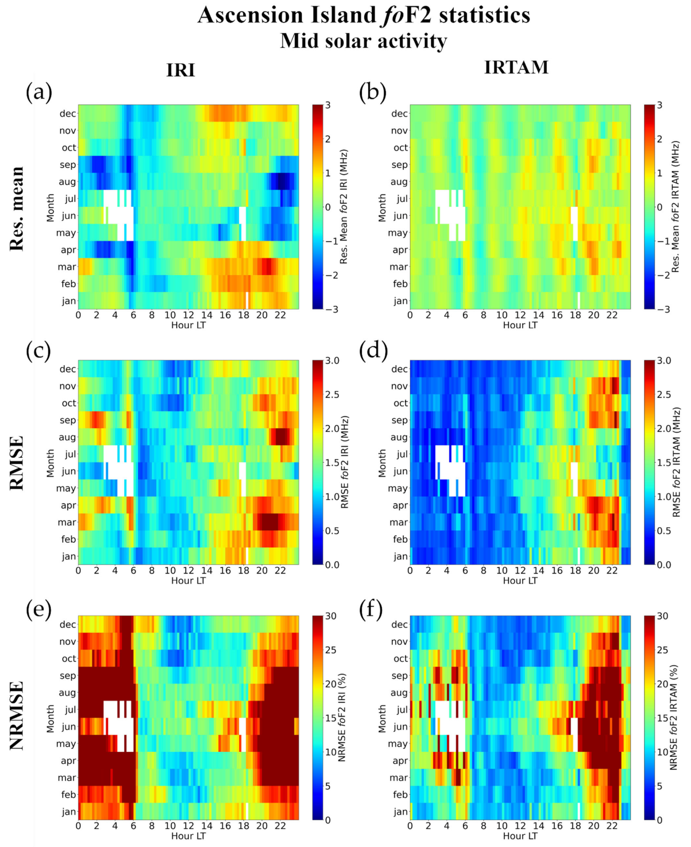
  • Ascension Island (low-latitude station, QD lat. = 19.1° S, Figure 7, Figure 8 and Figure 9): it was chosen because among the low-latitude stations characterized by a mid-low modip (modip = 34.3° S) it is the one that presents the longest dataset (264,916 measurements); it has also the particularity to lay over the southern equatorial anomaly crest.
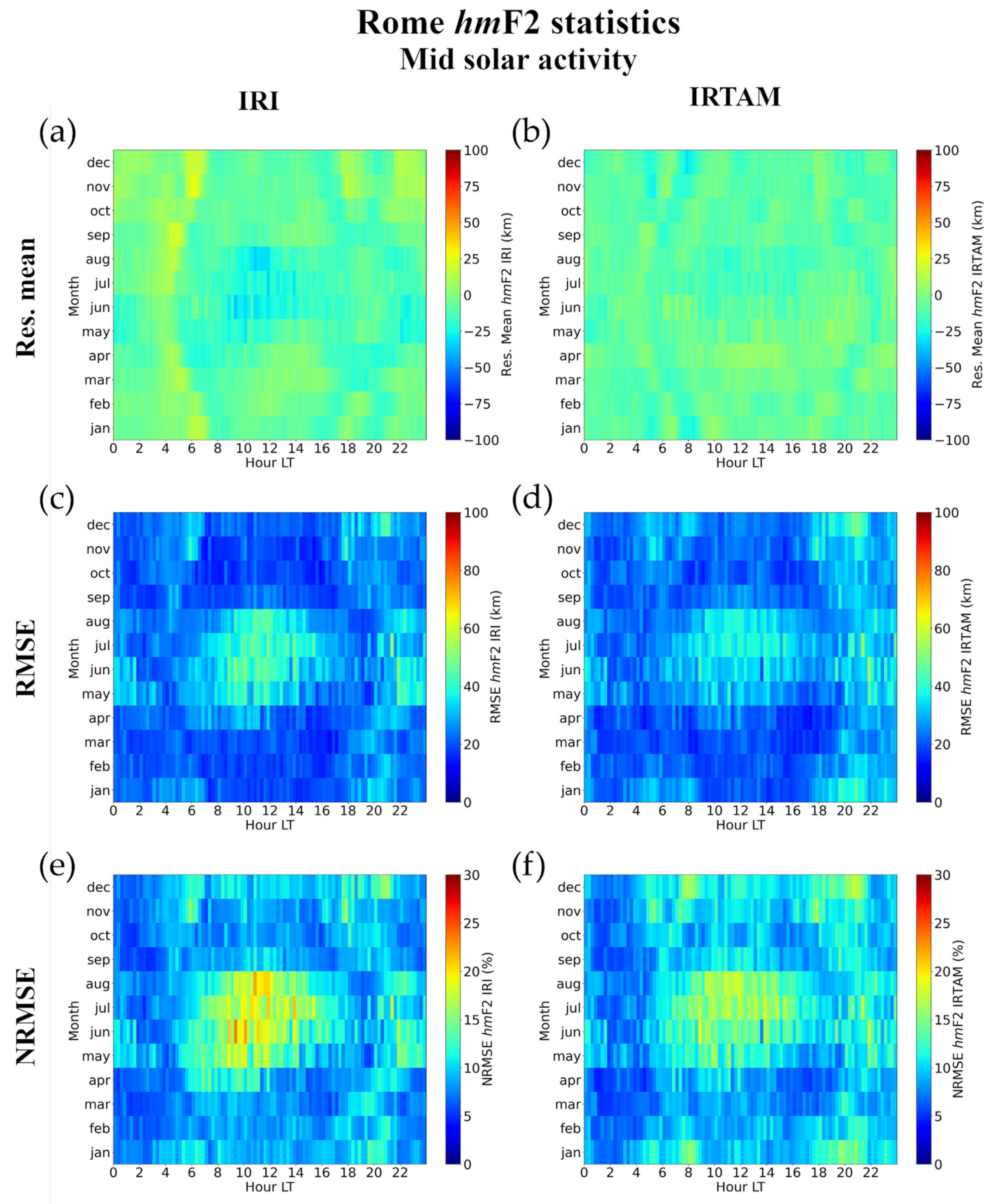
  • Rome (mid-latitude station, QD lat. = 35.9° N, Figure 10, Figure 11 and Figure 12): it was chosen because among the mid-latitude stations characterized by a mid modip (modip = 49.3° N) it is the one that presents the longest dataset, which is also the longest dataset among the 40 considered stations (520,519 measurements).
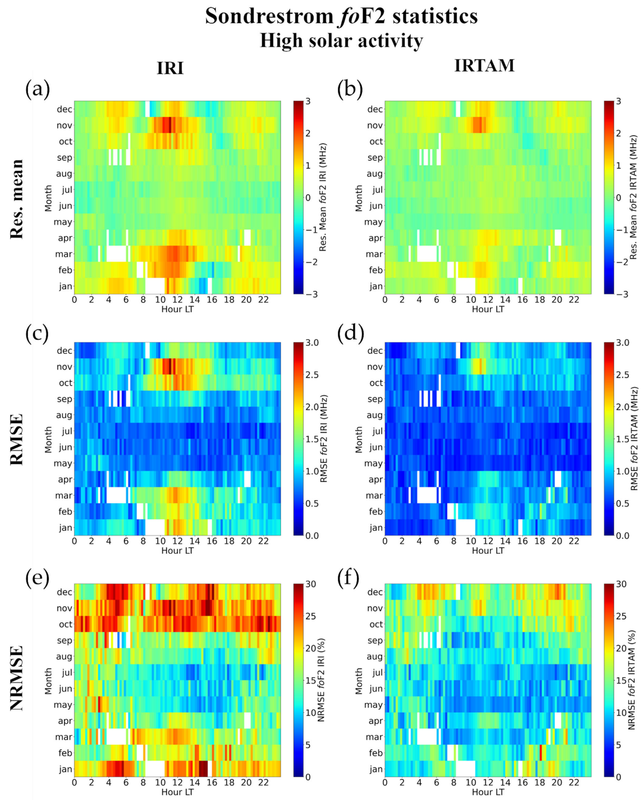
  • Sondrestrom (high latitude, QD lat. = 72.2° N, Figure 13, Figure 14 and Figure 15): it was preferred among the stations with high modip (modip = 65.8° N) even if it presents a dataset that is a little bit shorter (200,111 measurements) than that of Tromso (259,000 measurements). The reason for this choice lies in the fact that Sondrestrom is significantly higher in latitude than Tromso (QD lat. = 66.5° N) and, thus, more representative of the auroral latitudes.
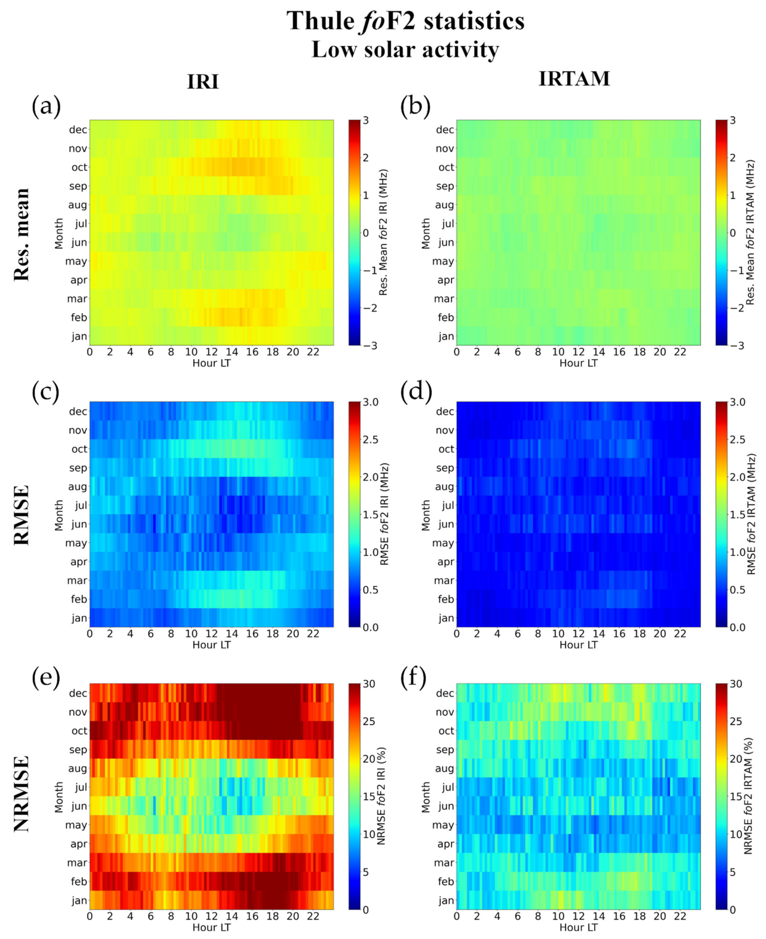
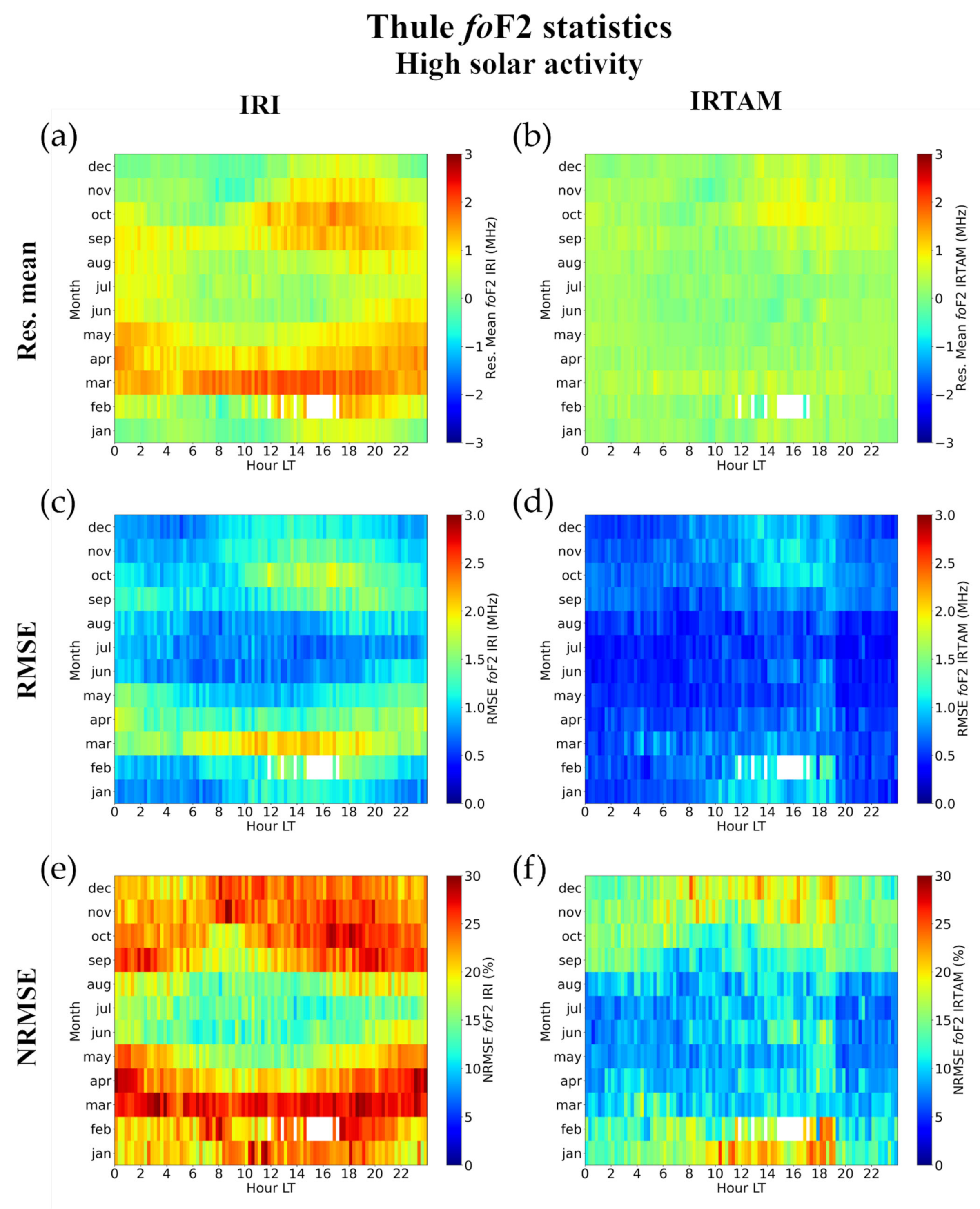
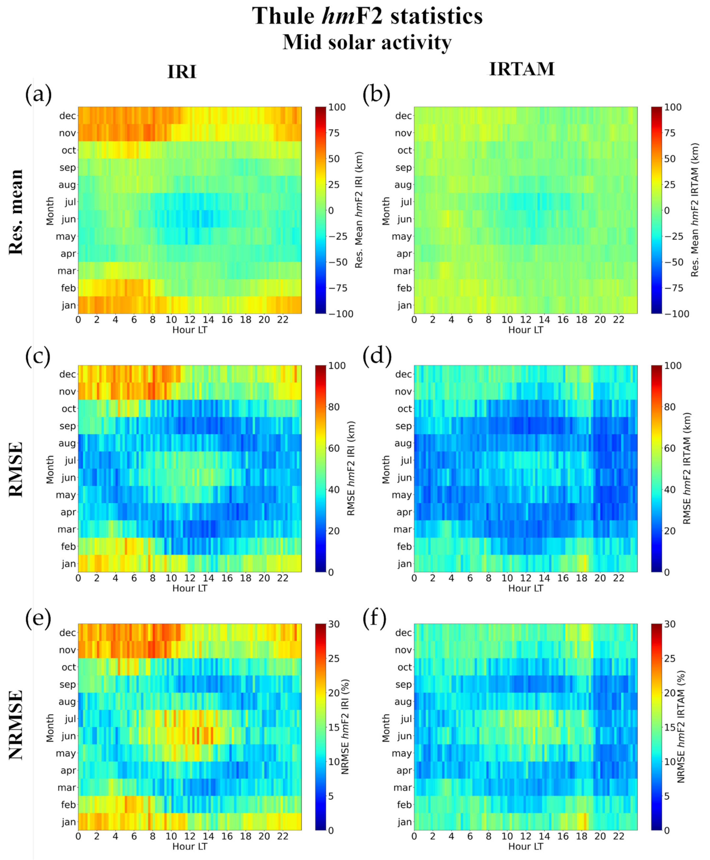
  • Thule (polar cap, QD lat. = 84.5° N, Figure 16, Figure 17 and Figure 18): it was chosen among the stations with very high modip (modip = 72.7° N) because it provides a dataset (278,374 measurements) substantially larger than that of Nord Greenland (47,039 measurements), and also because of its proximity to the north pole.
In order to simplify the IRI-IRTAM comparison to the reader, all figures have been generated with the same scale. Since the main goal of the paper is the comparison between IRI and IRTAM performances, we will focus on the differences between the statistical metrics provided by IRI and IRTAM, without going into detail about the corresponding physical and theoretical explanation of the observed trends.
Figure 4, Figure 5 and Figure 6 show that at Jicamarca for LSA, IRTAM models foF2 more accurately than IRI, especially during pre-sunrise and post-sunset hours. An improvement in the foF2 modeling accuracy made by IRTAM is still observed for MSA around sunrise hours for equinoctial and summer months and during daytime hours for some equinoctial months. For both LSA and MSA, at sunrise both models show high percentages of error (at least 25%). Nevertheless, during nighttime, a significant reduction in the percentage error made by IRTAM can be appreciated, which means a good improvement in the foF2 modeling precision. For HSA, around sunrise in equinoctial and summer months, IRTAM performs better than IRI in terms of accuracy. The relatively high absolute errors (at least 2.0 MHz) made by IRI in equinoctial and summer months are strongly smoothed by IRTAM. Except for the hours around sunrise, where the percentage error remains pretty high (at least 25%), a very strong reduction in the percentage error made by IRTAM is observed in all seasons, which means a considerable improvement in the foF2 modeling precision.
Figure 7, Figure 8 and Figure 9 show that at Ascension Island overall, for LSA, during daytime hours and for all seasons, IRI models foF2 less accurately than IRTAM. A very similar behavior of the two models is observed for the absolute error. However, during the central hours of the day, IRTAM provides a greater foF2 modeling precision, being its percentage errors lower than those of IRI. Overall, for both MSA and HSA, the comparison between IRI and IRTAM Res. Mean grids suggests that IRI is less accurate than IRTAM. The IRTAM model reduces both the absolute and the percentage error, during the first hours of the night and daytime hours, which highlights an improvement in the IRI foF2 modeling precision. Both IRI and IRTAM provide bad performance during post-sunset hours, for which extremely high percentage errors, up to 30% and more, are observed.
Figure 10, Figure 11 and Figure 12 show that at Rome for LSA, a better performance in terms of foF2 modeling accuracy is clearly observed in favour of IRTAM, while RMSE and NRMSE grids show very similar patterns, thus indicating that the precision with which IRI and IRTAM model foF2 is comparable. Overall, for MSA, IRI and IRTAM performances are comparable in terms of accuracy. For HSA, a greater accuracy is provided by IRTAM, during pre-sunrise hours and daytime hours for summer months. For both MSA and HSA, the IRTAM model lowers the values of the absolute and percentage errors, which means that an improvement in the foF2 modeling precision is achieved.
Figure 13, Figure 14, Figure 15, Figure 16, Figure 17 and Figure 18 show that at Sondrestrom and Thule for the three considered solar activity levels a remarkable reduction in the Res. Mean, RMSE, and NRMSE values is observed when passing from IRI to IRTAM, which means that a significant improvement in the foF2 modeling is achieved in terms of both accuracy and precision. The improvement brought by IRTAM is remarkable at equinoctial and winter months.
From a visual inspection of foF2 grids obtained for the three solar activity ranges, some general considerations on how the IRI and IRTAM performances depend on solar activity can be made: no clear Res. Mean trend related to the solar activity for both IRI and IRTAM is found; IRI and IRTAM models show an increasing RMSE trend as the solar activity increases; a clear decreasing NRMSE trend is detected as the solar activity increases at Jicamarca, Ascension Island, and Rome for IRTAM, and at Thule and Sondrestrom for IRI. For the other cases it is difficult to establish a clear solar activity dependence. However, patterns characterized by higher NMRSE are almost always observed for lower solar activity.

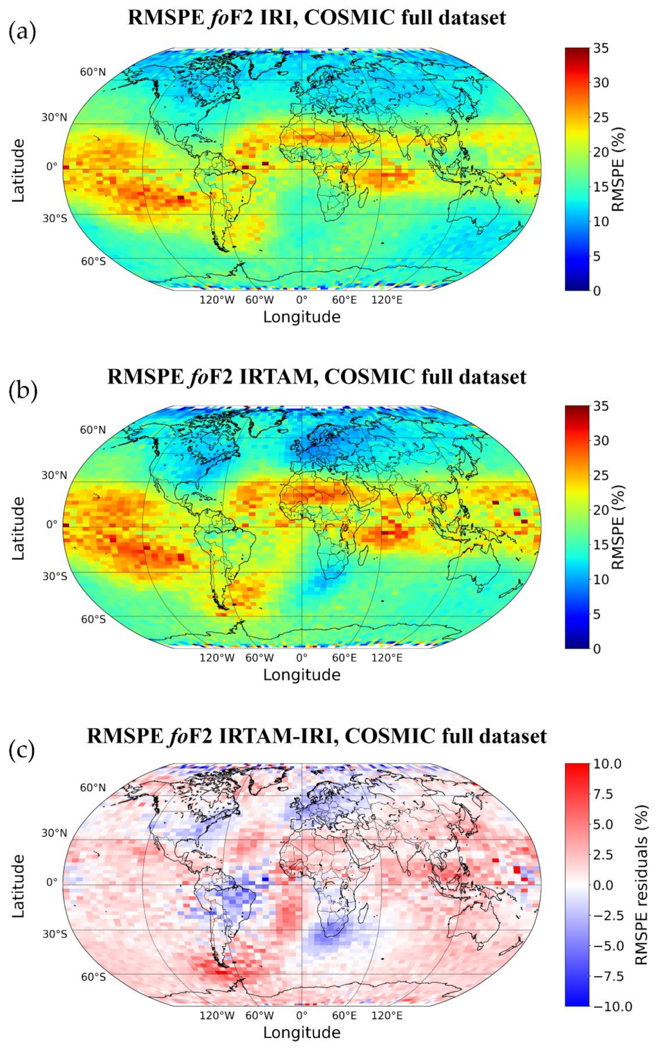
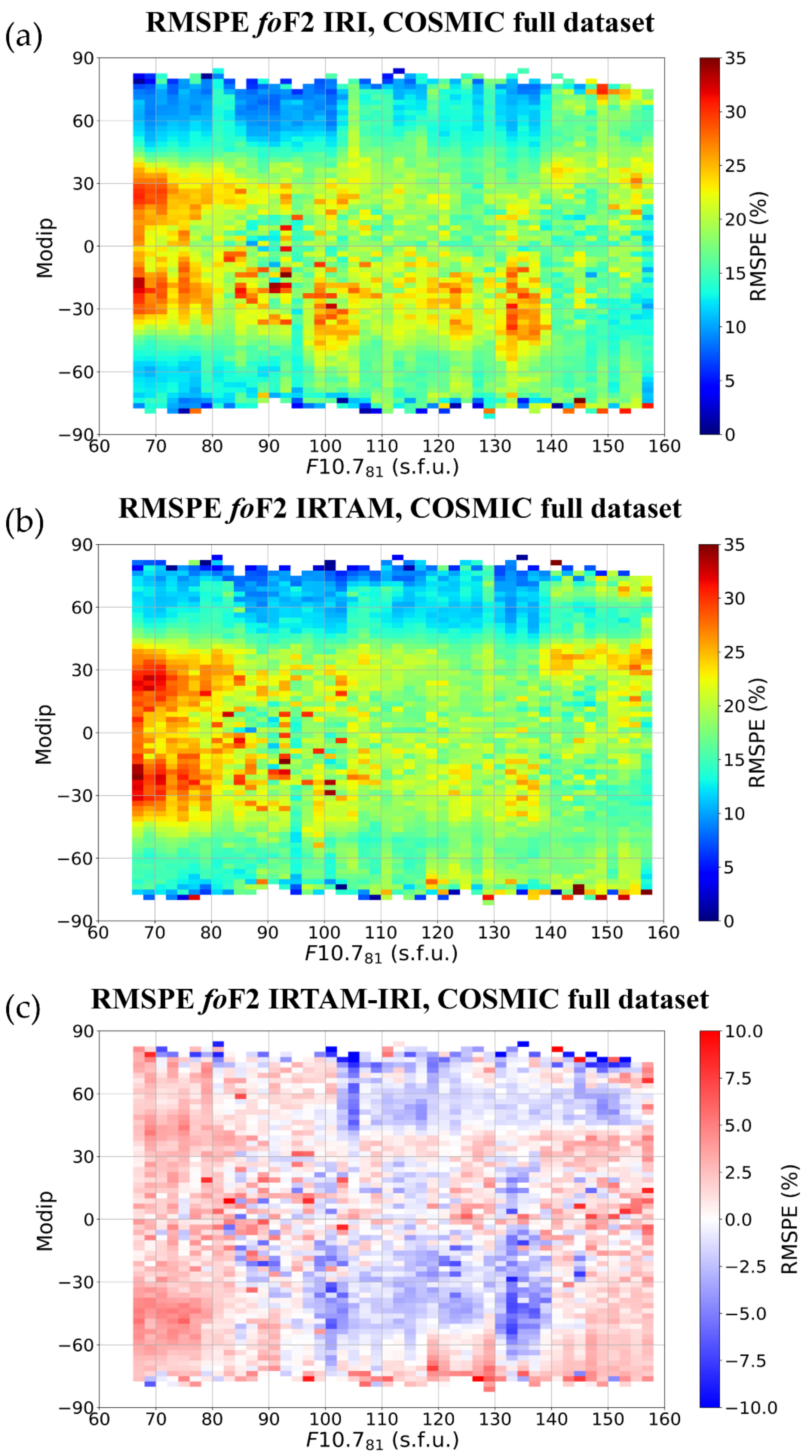
6. Validation Results for foF2 Based on Radio Occultation Observations

The full COSMIC dataset, comprising 1,791,602 selected electron density profiles measured from 2006 to 2018, was used to retrieve reliable foF2 values for calculating the two-dimensional density plots of IRI-foF2 vs. COSMIC-foF2 and IRTAM-foF2 vs. COSMIC-foF2, along with the histograms of corresponding residuals, as shown in Figure 19. Differently from Figure 3, Figure 19 shows that IRTAM does not improve the foF2 modeling accuracy of IRI. In fact, the IRTAM statistical distribution of residuals around the zero value, very similar to the IRI one, shows a value of Res. MeanIRTAM = 0.095 MHz that is a little bit greater than Res. MeanIRI = 0.067 MHz.
Moreover, the comparisons RMSEIRTAM = 1.120 MHz vs. RMSEIRI = 1.053 MHz and NRMSEIRTAM = 17.748% vs. NRMSEIRI = 16.668% show a slight worsening of the foF2 modeling precision made by IRTAM. This is also supported by the IRTAM density plot which appears more scattered than the IRI one (RIRTAM = 0.888 vs. RIRI = 0.901). However, given that the statistical quantities calculated with the two models do not differ significantly, we can claim that the IRI and IRTAM performances based on the COSMIC foF2 data can be considered somewhat comparable.
The statistical results reported in the following Table 4 show that only in a few cases is Res. MeanIRTAM < Res. MeanIRI, while in all cases RMSEIRI < RMSEIRTAM, NRMSEIRI < NRMSEIRTAM, and RIRI > RIRTAM. This means that the same concerns held for the entire COSMIC foF2 dataset (Figure 19) hold also when IRI and IRTAM performances are evaluated on the COSMIC foF2 time series binned according to the procedures described in Section 4.2, and considering the three levels of solar activity defined in Section 3.1.
In order to provide a comprehensive picture of how IRI and IRTAM models behave when the COSMIC foF2 dataset is considered for validation, global maps of IRI and IRTAM RMSPE values were calculated along with the corresponding maps of the differences (RMSPEIRTAMRMSPEIRI). It is important to note that for validating both models in terms of spatial, diurnal, seasonal, and solar activity variability, the maps were calculated binning IRI, IRTAM and (IRTAM-IRI) RMSPE values as a function of: geographic latitude vs. geographic longitude, modip vs. LT hour, modip vs. doy, and modip vs. F10.781 (see Figure 20, Figure 21, Figure 22 and Figure 23).
Figure 20 highlights significant differences between the two models. Specifically, the actual ionospheric conditions are better represented by IRTAM over those areas where a high concentration of ionosondes is available for data assimilation. Specifically, a clear improvement in the foF2 modeling is observed over Europe, South Africa, North America, and Brazil, where the RMSPE percentage error is remarkably reduced when IRTAM is run. Vice versa, over the oceans, deserts (e.g., Sahara, Gobi, Kalahari) and Antarctica as well, a better performance from the IRI side is observed. These circumstances can explain why the results of Figure 19 show a global balance between the two models. As expected from an assimilative model, IRTAM improves considerably IRI predictions over those regions where it is possible to assimilate a large number of data. However, a little unexpected is the observed situation that IRTAM does not seem to reproduce the IRI background in areas very far away from the assimilation sites, which is a constraint that it is usually requested by an assimilative model (see, for example, [11,14]). In fact, since IRTAM works on the residuals between measured values and IRI values through NECTAR (see Section 2.2), it should correct the background model close to assimilation sites and relax to the background far away from assimilation sites. This is not the case represented in Figure 20. A possible explanation of this could lay on the global nature of the correction made by IRTAM to URSI coefficients. In fact, even if the diurnal correction is maximum at assimilation sites (Section 2.2), corrected diurnal coefficients are used to calculate the corrected spatial coefficients through the Jones and Gallet procedure; as a consequence, the correction affects the spatial harmonic functions that have a global nature. Because of this, the effect of the correction at one assimilation site can influence also a very distant location. On the one hand, this is a clear advantage because the correction has a global nature and is robust against sporadic data outliers but, on the other hand, the quality of the procedure critically depends on the spatial distribution of assimilation sites. It is clear from Figure 20 that the current Digisondes’ global distribution is an important constraint for IRTAM. This accounts for the IRTAM performances that are better at mid latitudes than at low latitudes, as visible in Figure 20, Figure 21, Figure 22 and Figure 23.
Figure 21 shows that IRI and IRTAM RMSPE maps obtained as a function of modip and local time are very similar: (a) both IRI and IRTAM show the best performance during daytime hours at northern high latitudes; (b) a worsening of both IRI and IRTAM performance is detected during the central hours of the day around 30° N; (c) the highest absolute and percentage errors occur in the latitudinal band (30° S, 30° N) around sunrise hours. This last circumstance was somehow expected from the IRI side because, being an empirical climatological model, IRI can have some limitations in describing the variability of the ionospheric characteristics when they present wide variations in a relatively small time window, as is the case at solar terminator hours. Nonetheless, the bottom panel of Figure 21 tells us that between 30° S and 30° N IRI performance was noticeably improved by IRTAM around sunrise hours. This fact constitutes a clear evidence of how data assimilation can play a key role in improving foF2 modeling in certain situations. Both models exhibit quite large errors during nighttime at mid-low latitudes, as already evidenced by Jicamarca and Ascension Islands grids (Figure 4, Figure 5, Figure 6, Figure 7, Figure 8 and Figure 9).
Figure 22 shows that from a seasonal point of view the performances of IRI and IRTAM are similar. Both models show most of the problems at low/equatorial latitudes throughout the year, especially in correspondence to the crests of the equatorial ionospheric anomaly, mostly the southern one. For what concerns the northern crest the output of IRI seems to be better than the IRTAM one. At mid and high latitudes, the seasonal dependence of the error associated with both models is remarkable, with lowest errors during summer months and highest during winter months.
Figure 23 shows the IRI and IRTAM RMSPE maps obtained as a function of modip and the solar activity. This figure highlights a clear improvement of the IRI performance made by IRTAM only for MSA conditions. The poor results observed for LSA from the IRI side were expected, because the conditions characterizing the solar minimum in 2008/2009 [64,65], much lower and prolonged than earlier minima, represented a challenge for IRI [66,67,68]. At the same time, it is somewhat unexpected that IRTAM cannot improve the IRI output for LSA, even though the model assimilates foF2 values that well represent the very low solar activity conditions of that period. As seen before, most of the improvement made by IRTAM is narrowed to mid latitudes.

7. Validation Results for hmF2 Based on Ground-Based Ionosonde Observations

7.1. Statistics on the Full Dataset

The full hmF2 ionosonde dataset comprises 10,133,987 measurements obtained cumulating time series recorded from 2000 to 2019 at the 40 considered ionospheric stations. This dataset has been used to calculate the two-dimensional density plots of IRI-hmF2 vs. ionosonde-hmF2 and IRTAM-hmF2 vs. ionosonde-hmF2, along with the histograms of corresponding residuals, as shown in Figure 24.
The comparison between IRI and IRTAM highlights that the IRTAM model slightly improves the hmF2 modeling accuracy. In fact, the IRTAM and IRI statistical distributions of residuals around the zero value are very similar and, on the other hand, Res. MeanIRTAM = −1.619 km is just a little bit smaller than Res. MeanIRI = 1.804 km. Additionally, the comparisons RMSEIRTAM = 27.965 km vs. RMSEIRI = 32.993 km and NRMSEIRTAM = 10.097% vs. RMSEIRI = 11.912% testify a slight improvement of the hmF2 modeling precision made by IRTAM. This point is also supported by the IRTAM density plot and the correlation coefficient (RIRTAM = 0.845 vs. RIRI = 0.766).
Compared to the foF2 results (ionosonde dataset, Figure 3), in this case the improvement made by IRTAM is lower. However, we have to consider that, for what concerns hmF2, IRTAM cannot be considered as a direct updating of IRI because of the Brunini procedure [53] for mapping hmF2 (see Section 2.2) and, more importantly, because we applied the current default hmF2 IRI option, i.e., that of Shubin et al. [44]. Hence, IRI and IRTAM hmF2 models have to be considered as completely unrelated.
Overall, the statistical results reported in Table 5 show that IRTAM models hmF2 better than IRI in terms both of accuracy and precision, although the degree of improvement is lower than that obtained for foF2 (Table 2).
Table 6 shows the statistical parameters (1–4) calculated for the hmF2 time series recorded in each of the 40 ionosonde stations listed in Table 1. Differently from the foF2 results shown in Table 3, the number of cases for which Res.MeanIRI < Res.MeanIRTAM and for which Res.MeanIRTAM < Res.MeanIRI is practically the same. This circumstance is in accordance with the very similar IRI (1.804 km) and IRTAM (−1.619 km) Res.Mean absolute values calculated when the whole hmF2 ionosonde dataset is considered (bottom row of Table 5). This fact points out that the two models are practically equivalent in terms of accuracy. Nonetheless, the IRTAM RMSE and NRMSE values are always lower than the IRI ones, with the exception of the stations of Anyang and I-Cheon, Kwajalein, and Rome. This fact highlights that IRTAM models hmF2 with a precision better than that of IRI.

7.2. Diurnal, Seasonal, and Solar Activity Statistics Variations for Different Zonal Sectors

The same criteria described in Section 5.2 for the selection of the ionospheric stations and the validation of the results based on ground-based foF2 ionosonde observations, were also adopted to validate the results of IRI and IRTAM models for hmF2. Therefore, as done in Section 5.2, the statistical grids for the same five ionospheric stations previously selected are shown in Figure 25, Figure 26, Figure 27, Figure 28, Figure 29, Figure 30, Figure 31, Figure 32, Figure 33, Figure 34, Figure 35, Figure 36, Figure 37, Figure 38 and Figure 39 for hmF2.
Figure 25, Figure 26 and Figure 27 show that at Jicamarca, for the three considered solar activity levels, IRTAM presents lower values of Res. Mean, RMSE, and NRMSE than IRI, which means that IRTAM improves the IRI hmF2 modeling in terms of both accuracy and precision. This improvement is observed mostly around sunrise and post-sunset hours. Moreover, IRTAM reduces the error made by IRI in the hmF2 modeling around noon in summer.
Figure 28, Figure 29 and Figure 30 show that at Ascension Island, for the three considered solar activity levels, the IRI hmF2 modeling accuracy is improved by IRTAM especially during nighttime hours. Overall, for LSA, the hmF2 modeling precision of IRI and IRTAM can be considered equivalent during pre-sunrise and daytime hours, since the RMSE and NRMSE grids at these hours show similar patterns. IRI instead shows a better output during post-sunset hours. For MSA and HSA, concerning the modeling precision, a better performance of IRI is observed during pre-sunrise hours.
Figure 31, Figure 32 and Figure 33 show that overall at Rome, for the three considered solar activity levels, IRTAM improves the IRI modeling accuracy, in particular for sunrise and daytime hours in summer. Concerning the modeling precision, both models are somewhat equivalent independently of solar activity. Nonetheless, a slight improvement made by IRTAM is found during the central hours of the day for summer months.
Figure 34, Figure 35 and Figure 36 show that at Sondrestrom, for LSA and MSA, the IRI hmF2 modeling accuracy during post-sunset hours is remarkably improved by IRTAM, in particular for winter and equinoctial months. Nevertheless, a worsening of IRTAM performance is observed during pre-sunrise hours in winter. For HSA, a drop of the hmF2 modeling accuracy is observed from the IRTAM side during daytime hours in summer. For LSA and MSA, RMSE and NRMSE grids show very similar patterns, thus indicating that the precision with which IRI and IRTAM model hmF2 is on the whole comparable. Nevertheless, it must be pointed out that a clear improvement when passing from IRI to IRTAM is observed during post-sunset hours in winter.
Figure 37, Figure 38 and Figure 39 show that at Thule, for the three considered solar activity levels, a considerable improvement in the hmF2 modeling accuracy is achieved by IRTAM during the whole day especially in winter and equinoctial months. Overall, RMSE and NRMSE grids show that IRTAM improves the hmF2 modeling precision, independently of solar activity. In particular, the improvement is appreciated during the whole day in winter and during daytime hours in summer.
From a visual examination of hmF2 grids achieved for the three solar activity ranges, some generic conclusions on how the IRI and IRTAM performances depend on solar activity can be drawn: no clear Res. Mean trend related to the solar activity for both IRI and IRTAM is found; neither IRI nor IRTAM show a clear RMSE trend related to the solar activity; for both models, a decreasing NRMSE trend is observed as the solar activity increases.

8. Validation Results for hmF2 Based on Radio Occultation Observations

The full COSMIC dataset, comprising 1,791,602 electron density profiles measured from 2006 to 2018, was used to retrieve reliable COSMIC hmF2 values for calculating the two-dimensional density plots of IRI-hmF2 vs. COSMIC-hmF2 and IRTAM-hmF2 vs. COSMIC-hmF2, along with the histograms of corresponding residuals, as shown in Figure 40. The figure shows that IRTAM slightly improves the hmF2 modeling accuracy because Res. MeanIRTAM = 0.140 km is smaller than Res. MeanIRI = 3.728 km.
The same cannot be said for the hmF2 modeling precision. In fact, the comparisons RMSEIRTAM = 32.223 km vs. RMSEIRI = 22.446 km and NRMSEIRTAM = 11.609% vs. NRMSEIRI = 8.087% show that the IRTAM absolute and percentage errors are by far higher than those of IRI. Moreover, the IRTAM density plot appears much more scattered than that of IRI (RIRTAM = 0.733 vs. RIRI = 0.881).
The statistical results reported in Table 7 show that in some cases Res. MeanIRTAM < Res. MeanIRI, while in many cases RMSEIRTAM > RMSEIRI, NRMSEIRTAM > NRMSEIRI, and RIRTAM < RIRI, which means that the same considerations made for the full COSMIC hmF2 dataset hold also when IRI and IRTAM performances are evaluated according to the procedures described in Section 4.2, considering the three levels of solar activity defined in Section 3.1.
Analogously to what was carried out in Section 6 for foF2, a global picture of the IRI and IRTAM behavior relative to the COSMIC hmF2 dataset is shown in Figure 41, Figure 42, Figure 43 and Figure 44.
Figure 40 shows that, differently from foF2, the values of RMSEIRI and NRMSEIRI calculated for hmF2 are relatively smaller than those of RMSEIRTAM and NRMSEIRTAM. This is reflected also in the distribution of residuals that in the case of IRTAM appears more widespread around the zero than that of IRI, and this has a strong impact on the maps shown in Figure 41, Figure 42, Figure 43 and Figure 44. In fact, these maps clearly highlight how IRTAM, independently of the analysis (spatial, diurnal, seasonal, and dependent on solar activity), does not improve the hmF2 modeling made by IRI. This result might be affected to a some extent by the fact that IRI hmF2 values have been calculated through the Shubin et al. [44] model, which is partly based on electron density profiles collected by COSMIC between 2006 and 2012.

9. Final Analyses and Comparisons between IRI and IRTAM

The results shown in the previous sections are here summarized through the residual deviation ratio Rcw defined in Section 4. Rcw is a statistical parameter that in general is very suitable to assess definitively the performance of one model over another. To this end, the IRI and IRTAM performances are evaluated analyzing the distributions (in a logarithmic scale) of the residuals’ deviation ratio calculated on both the full foF2 ionosonde/COSMIC dataset (Figure 45) and the full hmF2 ionosonde/COSMIC dataset (Figure 46).
The log10(Rcw) distribution shown in Figure 45a is clearly “shifted” towards the positive values. Specifically, the mean value of the distribution equal to +0.212 highlights that overall IRTAM performs better than IRI by a factor of about 1.6 when considering the foF2 ionosonde dataset. Instead, the log10(Rcw) distribution shown in Figure 45b is quite symmetric with respect to the zero value. This fact is strongly supported by the mean value of the distribution, which is equal to −0.001. Therefore, the IRI and IRTAM performances can be considered equivalent when considering the COSMIC foF2 dataset.
The log10(Rcw) distribution shown in Figure 46a is quite symmetric around the zero. Specifically, the mean value of the distribution equal to +0.057 (which corresponds to an improvement factor of about 1.14) highlights that IRTAM and IRI provide quite comparable outputs when considering the hmF2 ionosonde dataset. The log10(Rcw) distribution shown in Figure 46b is clearly “shifted” towards the negative values. Specifically, the mean value of the distribution equal to −0.188 points out that IRI performs better than IRTAM when considering the hmF2 COSMIC dataset by a factor of about 1.5.
The same analysis based on log10(Rcw) distribution was applied by Galkin et al. [18] on a dataset of foF2 values recorded by 59 ionosondes during May–June 2019. They found results very similar to the ones shown in Figure 45a, with IRTAM improving IRI by a factor of about two (about 0.3 in the logarithmic scale of Figure 45). The slight differences are due on the one hand to the fact that to test IRTAM Galkin et al. [18] used only data from assimilated stations, while in this study we used also non-assimilated stations, and on the other hand to the larger extension of our dataset covering different seasons and solar activity levels. Results similar to those of Galkin et al. [18] were obtained also by Vesnin [29] by considering a larger dataset covering one solar cycle, but again using only data from assimilated stations to test the model. Vesnin [29] investigated the IRTAM performance also for hmF2 and found that IRTAM improved IRI by a factor of about 1.8. However, in that analysis the oldest Bilitza et al. [41] hmF2 IRI option was used as comparison. When using the newest Shubin et al. [44] default IRI hmF2 option, we find much lower differences between IRTAM and IRI, thus confirming the very important step forward made by IRI about the hmF2 modeling, as on the other hand recently outlined by different authors [69,70,71].
Figure 45 and Figure 46 confirm the general picture outlined by the analyses described in Section 5, Section 6, Section 7 and Section 8, i.e., the comparison with ionosonde data highlights how IRTAM significantly improves the foF2 prediction made by IRI, while for hmF2 the performances are quite similar between the two models. Since IRTAM assimilates both foF2 and hmF2 from the GIRO network, we would have expected a similar improvement also in the hmF2 prediction. Besides the obvious differences due to the application of the newest Shubin et al. [44] IRI hmF2 default option, two important points need to be highlighted. First, the IRTAM hmF2 description is based on the mapping procedure introduced by Brunini et al. [53], which introduces residuals in the range from −10 to 10 km when compared to the original hmF2 values obtained from the Bilitza et al. [41] formulation. The second point is inherent to the hmF2 derivation from ionograms. In fact, while foF2 is a parameter that is directly obtained from ionograms as the maximum ordinary frequency reflected by the ionosphere, hmF2 has to be derived trough a mathematical inversion procedure that, starting from critical frequencies measured at different virtual heights, allows obtaining the electron density values at real heights [72]. This inversion procedure is sensitive to different possible error sources due to the E-valley presence, the interpretation of the F2-layer cusp made by ARTIST, and in general the quality of the ionogram echo traces. All of these matters may represent possible sources of error, that are estimated in the order of 10 km [73]. From the above considerations, it clearly emerges that to obtain reliable hmF2 values is more difficult than to get foF2 ones, even with data assimilation. This is a point that requires further improvements and refining of both the data assimilation procedure and the measurement technique itself.
The comparison with the F2-layer peak characteristics derived from COSMIC RO showed a general worsening of the IRTAM performances in comparison with the IRI ones. Specifically, the comparison with the COSMIC dataset (Figure 20 and Figure 41) highlighted that IRTAM improves the IRI foF2 and hmF2 predictions mainly in regions characterized by a dense ionosonde network. This suggests the extent to which IRTAM is tied to data assimilated by ionosondes and to the corresponding spatial distribution. Since assimilated data are used by IRTAM to update the coefficients of the spherical harmonic analysis underlying the IRI description, we would have expected that the improvements were not restricted to the ionosondes’ locations but would embrace at least the whole latitudinal sector where assimilated ionosondes are located. Moreover, the IRTAM description should fade towards that of the IRI in regions where the effect of the assimilated data can be considered negligible. These two points are very important, impacting on IRTAM global performances, and need to be deeply investigated for future versions of IRTAM. Currently, IRTAM assimilates data from about 60 GIRO Digisondes. With the ever-increasing number of available Digisondes, able to provide real-time data, and as a consequence of their more homogeneous spatial distribution, a continuous improvement of the IRTAM performance is expected. However, even if in the future the availability of ionosonde data should increase for both the time resolution and the spatial coverage, the fact that IRTAM is so tied to the underlying IRI model (i.e., to the URSI formalism) represents a limit for the improvement and development of IRTAM itself. In fact, IRTAM through NECTAR, to minimize at assimilation sites the mismatch between measured and IRI modeled values, calculates the corrections to be added to the URSI coefficients, but the order of the diurnal and spatial harmonics is left unchanged. This means that steep spatial gradients and fast time variations that are below the limits that can be resolved with the current spatial and temporal resolution of the URSI formalism would not be represented by IRTAM, even with an increased availability of assimilated data. Since steep spatial gradients and fast time variations are customary under specific Space Weather conditions, and the aim of data-assimilation methods is the reliable representation of such conditions, this poses serious limitations for the IRTAM model that its developers should bear in mind in the future.

10. Conclusions

In the present paper, we compared the IRI and IRTAM models; the latter, being a real-time version of IRI, is based on the assimilation of ionosonde measurements. In order to assess the performance of the two models, two different datasets have been considered: (1) foF2 and hmF2 from ground-based ionosonde observations; (2) foF2 and hmF2 from space-based COSMIC RO observations. Through different analyses and comparison methodologies, we highlighted the main performances exhibited by both IRI and IRTAM for different locations and under different diurnal, seasonal, solar and magnetic activity conditions.
The main results of the study are:
  • When ionosonde observations are considered for validation, IRTAM improves significantly the IRI foF2 modeling while it slightly improves the IRI hmF2 modeling.
  • When COSMIC observations are considered for validation, IRTAM improves neither the IRI foF2 modeling nor the IRI hmF2 modeling.
These results highlight that IRTAM, in contrast to most of assimilation models, has ample room for improvement. The points that in our opinion deserve specific attention are: the bad performance of IRTAM when modeling foF2 at low latitudes; the global hmF2 modeling made by IRTAM which is often unreliable, especially in areas far away from the assimilating sites, where the representation made by IRTAM is at times really different from that of the IRI background; the fact that IRTAM performances are too dependent on the assimilated ionosondes location.
The improvement in the near real-time specification of the ionospheric F2-layer peak characteristics is becoming more and more important nowadays for telecommunication purposes and for Space Weather applications in general. For example, Hartman et al. [74] have recently applied IRTAM as the Floating Potential Measurement Unit (FPMU) back-up system that will be used to support the International Space Station (ISS) program. IRTAM foF2 maps were used by Froń et al. [75] to provide global maps of the ionospheric equivalent slab thickness (τ) parameter that are delivered through the GAMBIT Explorer software (http://giro.uml.edu/GAMBIT, accessed on 3 August 2021). An improved real-time specification of τ on a global basis is very important because this parameter describes the shape of the ionospheric electron density profile; thus, an improved specification of τ can help empirical models such as IRI in the description of the profile shape, especially the topside part [76,77,78,79].
Since in the incoming years the applications based on a near real-time specification of the ionospheric conditions will increase in number, an ever more reliable and robust representation of the ionosphere will become of outstanding importance. This is why near real-time data-assimilation models such as IRTAM need continuous improvement and refining, on the one hand to improve the climatological description of the ionosphere made by IRI, and on the other hand to pave the way for a reliable ionospheric weather description.

Author Contributions

Conceptualization, A.P., M.P. (Michael Pezzopane); methodology, A.P.; data curation, A.P.; investigation, all authors; validation, all authors; formal analysis, A.P.; writing—original draft preparation, A.P., M.P. (Marco Pietrella); writing—review and editing, all authors. All authors have read and agreed to the published version of the manuscript.

Funding

This research is partially supported by the Italian MIUR-PRIN grant 2017APKP7T on Circumterrestrial Environment: Impact of Sun-Earth Interaction.

Institutional Review Board Statement

Not applicable.

Informed Consent Statement

Not applicable.

Data Availability Statement

Data from ionospheric observatories are available via the public access portal of the Digital Ionogram Database (http://ulcar.uml.edu/DIDBase/, accessed on 3 August 2021) of the Global Ionosphere Radio Observatory in Lowell, MA. COSMIC/FORMOSAT-3 Radio Occultation data are available at the COSMIC Data Analysis and Archive Center (CDAAC, https://data.cosmic.ucar.edu/gnss-ro/cosmic1/, accessed on 3 August 2021). IRTAM Fortran package and GAMBIT coefficients are available at GAMBIT Consortium website (http://giro.uml.edu/GAMBIT/, accessed on 3 August 2021). IRI Fortran code is available at the IRI website (http://irimodel.org/, accessed on 3 August 2021). The ap magnetic activity index was downloaded from NASA’s Space Physics Data Facility of the Goddard Space Flight Center (https://spdf.gsfc.nasa.gov/pub/data/omni/high_res_omni/, accessed on 3 August 2021). The F10.7 solar index was downloaded through the OMNIWeb Data Explorer website (https://omniweb.gsfc.nasa.gov/form/dx1.html, accessed on 3 August 2021) maintained by the NASA.

Acknowledgments

This publication uses data from ionospheric observatories made available via the public access portal of the Digital Ionogram Database (http://ulcar.uml.edu/DIDBase/, accessed on 3 August 2021) of the Global Ionosphere Radio Observatory in Lowell, MA. The authors are indebted to the observatory directors and ionosonde operators for the significant investments of their time, effort, expertise, and funds needed to acquire and provide measurement data to academic research. The authors thank the COSMIC/FORMOSAT-3 team for making freely available Radio Occultation data through the COSMIC Data Analysis and Archive Center (CDAAC, https://data.cosmic.ucar.edu/gnss-ro/cosmic1/, accessed on 3 August 2021). Ivan Galkin and the entire GAMBIT Consortium (http://giro.uml.edu/GAMBIT/, accessed on 3 August 2021) are acknowledged for providing access to IRTAM computations (http://giro.uml.edu/IRTAM, accessed on 3 August 2021/), IRTAM Fortran package, and to the GAMBIT coefficients (https://ulcar.uml.edu/GAMBIT/GambitCoefficients/, accessed on 3 August 2021). The IRI team is acknowledged for developing and maintaining the IRI model and for giving access to the corresponding Fortran code via the IRI website (http://irimodel.org/, accessed on 3 August 2021). The ap magnetic activity index was downloaded from NASA’s Space Physics Data Facility of the Goddard Space Flight Center (https://spdf.gsfc.nasa.gov/pub/data/omni/high_res_omni/, accessed on 3 August 2021). The F10.7 solar index was downloaded through the OMNIWeb Data Explorer website (https://omniweb.gsfc.nasa.gov/form/dx1.html, accessed on 3 August 2021) maintained by the NASA.

Conflicts of Interest

The authors declare no conflict of interest.

Abbreviations

The following abbreviations are frequently used in this manuscript:
apPlanetary 3-h-range ap magnetic index
C-ScoreARTIST Confidence Score
CCIRConsultative Committee on International Radio
COSMICConstellation Observing System for Meteorology, Ionosphere and Climate/FORMOSAT-3 satellites
doyDay of the year
F10.7Daily solar radio flux at 10.7 cm
F10.78181-day running mean of the daily F10.7
foF2Ordinary critical frequency of the F2-layer
GAMBITGlobal Assimilative Model of Bottomside Ionosphere Timeline
GIROGlobal Ionospheric Radio Observatory
GPS Global Positioning System
hmF2Height of the F2-layer peak
HSAHigh solar activity
IRIInternational Reference Ionosphere
IRTAMIRI Real-Time Assimilative Mapping
LSALow solar activity
LTLocal Time
M(3000)F2Ionospheric propagation factor
ModipModified dip latitude
MSAMid solar activity
NECTARNon-linear Error Compensation Technique for Associative Restoration
NRMSENormalized root mean square error
QD Quasi Dipole
RPearson correlation coefficient
RcwResiduals deviation ratio parameter
Res. MeanMean of residuals
RMSERoot mean square error
RMSPERoot mean square percentage error
RORadio occultation
SZASolar zenith angle
vTECvertical Total Electron Content
URSI International Union of Radio Science
UT Universal Time

References

  1. Moldwin, M. An Introduction To Space Weather; Cambridge University Press: Cambridge, MA, USA, 2008. [Google Scholar] [CrossRef]
  2. Cander, L.R. Ionospheric Space Weather; Springer Nature: Cham, Switzerland, 2019. [Google Scholar] [CrossRef]
  3. Schunk, R.W.; Scherliess, L.; Sojka, J.J.; Thompson, D.C.; Anderson, D.N.; Codrescu, M.; Minter, C.; Fuller-Rowell, T.J.; Heelis, R.A.; Hairston, M.; et al. Global assimilation of ionospheric measurements (GAIM). Radio Sci. 2004, 39. [Google Scholar] [CrossRef]
  4. Angling, M.J.; Khattatov, B. Comparative study of two assimilative models of the ionosphere. Radio Sci. 2006, 41. [Google Scholar] [CrossRef]
  5. Decker, D.T.; McNamara, L.F. Validation of ionospheric weather predicted by global assimilation of ionospheric measurements (GAIM) models. Radio Sci. 2007, 42, RS4017. [Google Scholar] [CrossRef] [Green Version]
  6. McNamara, L.F.; Decker, D.T.; Welsh, J.A.; Cole, D.G. Validation of the Utah State University global assimilation of ionospheric measurements (GAIM) model predictions of the maximum usable frequency for a 3000 km circuit. Radio Sci. 2007, 42, RS3015. [Google Scholar] [CrossRef]
  7. McNamara, L.F.; Bishop, G.J.; Welsh, J.A. Assimilation of ionosonde profiles into a global ionospheric model. Radio Sci. 2011, 46, RS2006. [Google Scholar] [CrossRef] [Green Version]
  8. Buresova, D.; Nava, B.; Galkin, I.; Angling, M.; Stankov, S.M.; Coisson, P. Data ingestion and assimilation in ionospheric models. Ann. Geophys. 2009, 52, 235–253. [Google Scholar] [CrossRef]
  9. Nava, B.; Coisson, P.; Radicella, S.M. A new version of the NeQuick ionosphere electron density model. J. Atmos. Sol. Terr. Phys. 2008, 70, 1856–1862. [Google Scholar] [CrossRef]
  10. Nava, B.; Radicella, S.M.; Azpilicueta, F. Data ingestion into NeQuick 2. Radio Sci. 2011, 46. [Google Scholar] [CrossRef] [Green Version]
  11. Pezzopane, M.; Pietrella, M.; Pignatelli, A.; Zolesi, B.; Cander, L.R. Assimilation of autoscaled data and regional and local ionospheric models as input sources for real-time 3-D international reference ionosphere modeling. Radio Sci. 2011, 46, 5009. [Google Scholar] [CrossRef] [Green Version]
  12. Pezzopane, M.; Pietrella, M.; Pignatelli, A.; Zolesi, B.; Cander, L.R. Testing the three-dimensional IRI-SIRMUP-P mapping of the ionosphere for disturbed periods. Adv. Space Res. 2013, 52, 1726–1736. [Google Scholar] [CrossRef] [Green Version]
  13. Shim, J.S.; Kuznetsova, M.; Rastatter, L.; Hesse, M.; Bilitza, D.; Butala, M.; Codrescu, M.; Emery, B.; Foster, B.; Fuller-Rowell, T.; et al. CEDAR electrodynamics thermosphere ionosphere (ETI) challenge for systematic assessment of ionosphere/thermosphere models: NmF2, hmF2, and vertical drift using ground-based observations. Space Weather 2011, 9, S12003. [Google Scholar] [CrossRef] [Green Version]
  14. Pignalberi, A.; Pezzopane, M.; Rizzi, R.; Galkin, I. Effective solar indices for ionospheric modeling: A review and a proposal for a real-time regional IRI. Surv. Geophys. 2018, 39, 125–167. [Google Scholar] [CrossRef]
  15. Pietrella, M.; Pignalberi, A.; Pezzopane, M.; Pignatelli, A.; Azzarone, A.; Rizzi, R. A comparative study of ionospheric IRIEup and ISP assimilative models during some intense and severe geomagnetic storms. Adv. Space Res. 2018, 61, 2569–2584. [Google Scholar] [CrossRef]
  16. Pietrella, M.; Pezzopane, M.; Zolesi, B.; Cander, L.R.; Pignalberi, A. The simplified ionospheric regional model (SIRM) for HF prediction: Basic theory, its evolution and applications. Surv. Geophys. 2020, 41, 1143–1178. [Google Scholar] [CrossRef]
  17. Galkin, I.A.; Reinisch, B.W.; Huang, X.; Bilitza, D. Assimilation of GIRO data into a real-time IRI. Radio Sci. 2012, 47. [Google Scholar] [CrossRef]
  18. Galkin, I.A.; Reinisch, B.W.; Vesnin, A.M.; Bilitza, D.; Fridman, S.; Habarulema, J.B.; Veliz, O. Assimilation of sparse continuous near-Earth weather measurements by NECTAR model morphing. Space Weather 2020, 18, e2020SW002463. [Google Scholar] [CrossRef]
  19. Bilitza, D.; Altadill, D.; Truhlik, V.; Shubin, V.; Galkin, I.; Reinisch, B.; Huang, X. International reference ionosphere 2016: From ionospheric climate to real-time weather predictions. Space Weather 2017, 15, 418–429. [Google Scholar] [CrossRef]
  20. Bilitza, D. IRI the international standard for the ionosphere. Adv. Radio Sci. 2018, 16, 1–11. [Google Scholar] [CrossRef] [Green Version]
  21. Lei, J.; Syndergaard, S.; Burns, A.G.; Solomon, S.C.; Wang, W.; Zeng, Z.; Roble, R.G.; Wu, Q.; Kuo, Y.-H.; Holt, J.M.; et al. Comparison of COSMIC ionospheric measurements with ground-based observations and model predictions: Preliminary results. J. Geophys. Res. 2007, 112, A07308. [Google Scholar] [CrossRef]
  22. Damboldt, T.; Suessmann, P. Information document on the analysis and validity of present ITU foF2 and M (3000) f2 maps. Int. Telecommun. Union 2011. question ITU-R 212-1/3. Available online: http://www.itu.int/md/R07-WP3L-C-0086/en (accessed on 3 August 2021).
  23. Shim, J.S.; Tsagouri, I.; Goncharenko, L.; Rastaetter, L.; Kuznetsova, M.; Bilitza, D.; Codrescu, M.; Coster, A.J.; Solomon, S.C.; Fedrizzi, M.; et al. Validation of ionospheric specifications during geomagnetic storms: TEC and foF2 during the 2013 March storm event. Space Weather 2018, 16, 1686–1701. [Google Scholar] [CrossRef] [Green Version]
  24. Shim, J.S.; Kuznetsova, M.; Rastätter, L.; Hesse, M.; Bilitza, D.; Butala, M.; Codrescu, M.; Emery, B.; Foster, B.; Fuller-Rowell, T.; et al. CEDAR electrodynamics thermosphere ionosphere (ETI) challenge for systematic assessment of ionosphere/thermosphere models: Electron density, neutral density, NmF2, and hmF2 using space based observations. Space Weather 2012, 10, S10004. [Google Scholar] [CrossRef] [Green Version]
  25. Pedatella, N.M.; Yue, X.; Schreiner, W.S. Comparison between GPS radio occultation electron densities and in situ satellite observations. Radio Sci. 2015, 50, 518–525. [Google Scholar] [CrossRef]
  26. Pignalberi, A.; Pezzopane, M.; Tozzi, R.; De Michelis, P.; Coco, I. Comparison between IRI and preliminary Swarm Langmuir probe measurements during the St. Patrick storm period. Earth Planets Space 2016, 68. [Google Scholar] [CrossRef] [Green Version]
  27. Tsagouri, I.; Goncharenko, L.; Shim, J.S.; Belehaki, A.; Buresova, D.; Kuznetsova, M.M. Assessment of current capabilities in modeling the ionospheric climatology for space weather applications: foF2 and hmF2. Space Weather 2018, 16, 1930–1945. [Google Scholar] [CrossRef] [Green Version]
  28. Cai, X.; Burns, A.G.; Wang, W.; Coster, A.; Qian, L.; Liu, J.; Solomon, S.C.; Eastes, R.W.; Daniell, R.E.; McClintock, W.E.; et al. Comparison of GOLD nighttime measurements with total electron content: Preliminary results. J. Geophys. Res. Space Phys. 2020, 125, e2019JA027767. [Google Scholar] [CrossRef]
  29. Vesnin, A.M. Validation of F2 Layer Peak Height and Density of Real-Time International Reference Ionosphere. Master’s Thesis, University of Massachusetts Lowell, Lowell, MA, USA, 2014. Available online: https://ulcar.uml.edu/GAMBIT/Vesnin-Master-thesis-2014.pdf (accessed on 3 August 2021).
  30. Zolesi, B.; Cander, L.R. Ionospheric Prediction and Forecasting; Springer: Berlin/Heidelberg, Germany, 2014. [Google Scholar] [CrossRef]
  31. Rush, C.M.; Fox, M.; Bilitza, D.; Davies, K.; McNamara, L.; Stewart, F.G.; PoKempner, M. Ionospheric mapping-an update of foF2 coefficients. Telecommun. J. 1989, 56, 179–182. [Google Scholar]
  32. Jones, W.B.; Gallet, R.M. Representation of diurnal and geographical variations of ionospheric data by numerical methods. Telecommun. J. 1962, 29, 129–149. Available online: https://nvlpubs.nist.gov/nistpubs/jres/66D/jresv66Dn4p419_A1b.pdf (accessed on 3 August 2021).
  33. Jones, W.B.; Gallet, R.M. Representation of diurnal and geographic variations of ionospheric data by numerical methods, II. Control of instability. Telecommun. J. 1965, 32, 18–28. [Google Scholar]
  34. Jones, W.B.; Graham, R.P.; Leftin, M. Advances in Ionospheric Mapping by Numerical Methods; ESSA Technical Report ERL107-ITS75; US Department of Commerce: Boulder, CO, USA, 1969. Available online: https://www.govinfo.gov/content/pkg/GOVPUB-C13-4811417984235af8236e56a8e5d5d483/pdf/GOVPUB-C13-4811417984235af8236e56a8e5d5d483.pdf (accessed on 3 August 2021).
  35. CCIR Atlas of Ionospheric Characteristics Report 340; Consultative Committee on International Radio, International Telecommunication Union: Geneva, Switzerland, 1967.
  36. Rawer, K. Propagation of decameter waves (HF Band). In Meteorological and Astronomical Influences on Radio Wave Propagation; Landmark, B., Ed.; Academic Press: New York, NY, USA, 1963; pp. 221–250. [Google Scholar]
  37. Liu, R.; Smith, P.; King, J. A new solar index which leads to improved foF2 predictions using the CCIR atlas. Telecomm. J. 1983, 50, 408–414. [Google Scholar]
  38. Fuller-Rowell, T.J.; Araujo-Pradere, E.; Codrescu, M.V. An empirical ionospheric storm-time correction model. Adv. Space Res. 2000, 25, 139–146. [Google Scholar] [CrossRef]
  39. Araujo-Pradere, E.A.; Fuller-Rowel, T.J.; Codrescu, M.V. STORM: An empirical storm-time ionospheric correction model 1. Model description. Radio Sci. 2002, 37. [Google Scholar] [CrossRef] [Green Version]
  40. Araujo-Pradere, E.A.; Fuller-Rowell, T.J. STORM: An empirical storm-time ionospheric correction model 2. Validation. Radio Sci. 2002, 37, 1071. [Google Scholar] [CrossRef]
  41. Bilitza, D.; Sheik, N.; Eyfrig, R. A global model for the height of the F2-peak using M3000 values from the CCIR numerical map. Telecommun. J. 1979, 46, 549–553. [Google Scholar]
  42. Altadill, D.; Magdaleno, S.; Torta, J.M.; Blanch, E. Global empirical models of the density peak height and of the equivalent scale height for quiet conditions. Adv. Space Res. 2013, 52, 1756–1769. [Google Scholar] [CrossRef]
  43. Shubin, V.N.; Karpachev, A.T.; Tsybuly, K.G. Global model of the F2 layer peak height for low solar activity based on GPS radio-occultation data. J. Atmos. Sol. Terr. Phys. 2013, 104, 106–115. [Google Scholar] [CrossRef]
  44. Shubin, V.N. Global median model of the F2-layer peak height based on ionospheric radio-occultation and ground based digisonde observations. Adv. Space Res. 2015, 56, 916–928. [Google Scholar] [CrossRef]
  45. Bilitza, D.; Bhardwaj, S.; Koblinsky, C. Improved IRI predictions for the GEOSAT time period. Adv. Space Res. 1997, 20, 1755–1760. [Google Scholar] [CrossRef]
  46. Komjathy, A.; Langley, R.; Bilitza, D. Ingesting GPS-derived TEC data into the international reference ionosphere for single frequency radar altimeter ionospheric delay corrections. Adv. Space Res. 1998, 22, 793–802. [Google Scholar] [CrossRef] [Green Version]
  47. Hernandez-Pajares, M.; Juan, J.; Sanz, J.; Bilitza, D. Combining GPS measurements and IRI model values for space weather specification. Adv. Space Res. 2002, 29, 949–958. [Google Scholar] [CrossRef]
  48. Ssessanga, N.; Kim, Y.H.; Kim, E.; Kim, J. Regional optimization of the IRI-2012 output (TEC, foF2) by using derived GPS-TEC. J. Korean Phys. Soc. 2015, 66, 1599–1610. [Google Scholar] [CrossRef]
  49. Habarulema, J.B.; Ssessanga, N. Adapting a climatology model to improve estimation of ionosphere parameters and subsequent validation with radio occultation and ionosonde data. Space Weather 2016, 15, 84–98. [Google Scholar] [CrossRef]
  50. Pignalberi, A.; Pezzopane, M.; Rizzi, R.; Galkin, I. Correction to: Effective solar indices for ionospheric modeling: A review and a proposal for a real-time regional IRI. Surv. Geophys. 2018, 39, 169. [Google Scholar] [CrossRef] [Green Version]
  51. Pignalberi, A.; Pietrella, M.; Pezzopane, M.; Rizzi, R. Improvements and validation of the IRI UP method under moderate, strong, and severe geomagnetic storms. Earth Planets Space 2018, 70, 1–22. [Google Scholar] [CrossRef]
  52. Pignalberi, A.; Habarulema, J.B.; Pezzopane, M.; Rizzi, R. On the development of a method for updating an empirical climatological ionospheric model by means of assimilated vTEC measurements from a GNSS receiver network. Space Weather 2019, 17, 1131–1164. [Google Scholar] [CrossRef] [Green Version]
  53. Brunini, C.; Conte, J.F.; Azpilicueta, F.; Bilitza, D. A different method to update monthly median hmF2 values. Adv. Space Res. 2013, 51, 2322–2332. [Google Scholar] [CrossRef]
  54. Hopfield, J.J. Neural networks and physical systems with emergent collective computational abilities. Proc. Natl. Acad. Sci. USA 1982, 79, 2554–2558. [Google Scholar] [CrossRef] [Green Version]
  55. Laundal, K.M.; Richmond, A.D. Magnetic Coordinate Systems. Space Sci. Rev. 2017, 206, 27. [Google Scholar] [CrossRef] [Green Version]
  56. Reinisch, B.W.; Galkin, I.A. Global Ionospheric Radio Observatory (GIRO). Earth Planets Space 2011, 63, 377–381. [Google Scholar] [CrossRef] [Green Version]
  57. Bibl, K.; Reinisch, B.W. The universal digital ionosonde. Radio Sci. 1978, 13, 519–530. [Google Scholar] [CrossRef]
  58. Galkin, I.A.; Reinisch, B.W. The new ARTIST 5 for all digisondes. In Ionosonde Network Advisory Group (INAG) Bulletin, 69th ed.; International Radio Science Union: Ghent, Belgium, 2008; Available online: http://www.ursi.org/files/CommissionWebsites/INAG/web-69/2008/artist5-inag.pdf (accessed on 3 August 2021).
  59. Galkin, I.A.; Reinisch, B.W.; Huang, X.; Khmyrov, G.M. Confidence score of ARTIST-5 ionogram autoscaling. In Ionosonde Network Advisory Group (INAG) Bulletin, 73rd ed.; International Radio Science Union: Ghent, Belgium, 2013; Available online: http://www.ursi.org/files/CommissionWebsites/INAG/web-73/confidence_score.pdf (accessed on 3 August 2021).
  60. Tapping, K.F. The 10.7 cm solar radio flux (F10.7): F10.7. Space Weather 2013, 11, 394–406. [Google Scholar] [CrossRef]
  61. Anthes, R.A.; Bernhardt, P.A.; Chen, Y.; Cucurull, L.; Dymond, K.F.; Ector, D.; Healy, S.B.; Ho, S.-P.; Hunt, D.C.; Kuo, Y.-H.; et al. The COSMIC/FORMOSAT-3 mission: Early results. Bull. Am. Meteorol. Soc. 2008, 89, 313–333. [Google Scholar] [CrossRef]
  62. Pignalberi, A.; Pezzopane, M.; Nava, B.; Coisson, P. On the link between the topside ionospheric effective scale height and the plasma ambipolar diffusion, theory and preliminary results. Sci. Rep. 2020, 10, 17541. [Google Scholar] [CrossRef]
  63. Rostoker, G. Geomagnetic indices. Rev. Geophys. Space Phys. 1972, 10, 935–950. [Google Scholar] [CrossRef]
  64. Solomon, S.C.; Woods, T.N.; Didkovsky, L.V.; Emmert, J.T.; Qian, L. Anomalously low solar extreme-ultraviolet irradiance and thermospheric density during solar minimum. Geophys. Res. Lett. 2010, 37, 16. [Google Scholar] [CrossRef]
  65. Perna, L.; Pezzopane, M. foF2 vs solar indices for the Rome station: Looking for the best general relation which is able to describe the anomalous minimum between cycles 23 and 24. J. Atmos. Space Phys. 2016, 146, 13–21. [Google Scholar] [CrossRef] [Green Version]
  66. Lühr, H.; Xiong, C. The IRI 2007 model overestimates electron density during the 23/24 solar minimum. Geophys. Res. Lett. 2010, 37, L23101. [Google Scholar] [CrossRef] [Green Version]
  67. Ezquer, R.G.; López, J.L.; Scidá, L.A.; Cabrera, M.A.; Zolesi, B.; Bianchi, C.; Pezzopane, M.; Zuccheretti, E.; Mosert, M. Behavior of ionospheric magnitudes of F2 region over Tucumán during a deep solar minimum and comparison with the IRI2012 model predictions. J. Atmos. Sol. Terr. Phys. 2014, 107, 89–98. [Google Scholar] [CrossRef]
  68. Perna, L.; Pezzopane, M.; Ezquer, R.; Cabrera, M.; Baskaradas, J.A. NmF2 trends at low and mid latitudes for the recent solar minima and comparison with IRI-2012 model. Adv. Space Res. 2017, 60, 363–374. [Google Scholar] [CrossRef]
  69. Arıkan, F.; Sezen, U.; Gulyaeva, T.L. Comparison of IRI-2016 F2 layer model parameters with ionosonde measurements. J. Geophys. Res. Space Phys. 2019, 124, 8092–8109. [Google Scholar] [CrossRef]
  70. Mengist, C.K.; Yadav, S.; Kotulak, K.; Bahar, A.; Zhang, S.-R.; Seo, K.-H. Validation of International Reference ionosphere model (IRI-2016) for F-region peak electron density height (hmF2): Comparison with Incoherent Scatter Radar (ISR) and ionosonde measurements at Millstone Hill. Adv. Space Res. 2020, 65, 2773–2781. [Google Scholar] [CrossRef]
  71. Huang, H.; Moses, M.; Volk, A.E.; Abu Elezz, O.; Kassamba, A.A.; Bilitza, D. Assessment of IRI-2016 hmF2 model options with digisonde, COSMIC and ISR observations for low and high solar flux conditions. Adv. Space Res. 2021. [Google Scholar] [CrossRef]
  72. Titheridge, J.E. Ionogram Analysis with the Generalised Program Polan, Rep. UAG-93; World Data Center A for Solar-Terrestrial Physics: Boulder, CO, USA, 1985. [Google Scholar]
  73. Chen, C.F.; Reinisch, B.W.; Scali, J.L.; Huang, X.; Gamache, R.R.; Buonsanto, M.J.; Ward, B.D. The accuracy of ionogram-derived N(h) profiles. Adv. Space Res. 1994, 14, 43–46. [Google Scholar] [CrossRef]
  74. Hartman, W.A.; Schmidl, W.D.; Mikatarian, R.; Galkin, I. Correlation of IRTAM and FPMU data confirming the application of IRTAM to support ISS Program safety. Adv. Space Res. 2019, 63, 1838–1844. [Google Scholar] [CrossRef]
  75. Froń, A.; Galkin, I.; Krankowski, A.; Bilitza, D.; Hernández-Pajares, M.; Reinisch, B.; Li, Z.; Kotulak, K.; Zakharenkova, I.; Cherniak, I.; et al. Towards cooperative global mapping of the ionosphere: Fusion feasibility for IGS and IRI with global climate VTEC maps. Remote Sens. 2020, 12, 3531. [Google Scholar] [CrossRef]
  76. Themens, D.R.; Jayachandran, P.T.; Bilitza, D.; Erickson, P.J.; Häggström, I.; Lyashenko, M.V.; Reid, B.; Varney, R.H.; Pustovalova, L. Topside electron density representations for middle and high latitudes: A topside parameterization for E-CHAIM based on the NeQuick. J. Geophys. Res. Space Phys. 2018, 123, 1603–1617. [Google Scholar] [CrossRef]
  77. Dos Santos Prol, F.; Themens, D.R.; Hernández-Pajares, M.; de Oliveira Camargo, P.; de Assis Honorato Muella, M.T. Linear vary-chap topside electron density model with topside sounder and radio-occultation data. Surv. Geophys. 2019, 40, 277. [Google Scholar] [CrossRef]
  78. Pezzopane, M.; Pignalberi, A. The ESA swarm mission to help ionospheric modeling: A new NeQuick topside formulation for mid-latitude regions. Sci. Rep. 2019, 9, 12253. [Google Scholar] [CrossRef] [Green Version]
  79. Pignalberi, A.; Pezzopane, M.; Themens, D.R.; Haralambous, H.; Nava, B.; Coïsson, P. On the analytical description of the topside ionosphere by NeQuick: Modeling the scale height through COSMIC/FORMOSAT-3 selected data. IEEE J. Sel. Top. Appl. Earth Obs. Remote. Sens. 2020, 13, 1867–1878. [Google Scholar] [CrossRef]
Figure 1. Global view of the ionosonde stations listed in Table 1. The yellow circles depict the ionosonde stations location with the corresponding identification number (Table 1, first column). Blue dashed curves depict the QD magnetic parallels, while red ones depict the modip parallels.
Atmosphere 12 01003 g001
Figure 2. (a) Percentage of available ionosonde observations per year and ionosonde station. (b) F10.781 time series from 2000 to 2019. Red horizontal dashed lines identify the three ranges chosen for the solar activity description.
Atmosphere 12 01003 g002
Figure 3. Density plots between measured (x-axis) and modeled (y-axis) foF2 values, for (a) IRI and (c) IRTAM. Measured values are those from the entire ionosonde dataset. The black solid lines represent the best linear fit. Corresponding slope and intercept values, along with the correlation coefficient, are reported in the upper left box of each plot. Statistical distributions of the resultant residuals for (b) IRI and (d) IRTAM. Corresponding Res. Mean, RMSE, and NRMSE values, along with the total number of counts on which the statistics is based, are reported in the upper left box of each plot.
Atmosphere 12 01003 g003
Figure 4. Grids of (a,b) Res. Mean, (c,d) RMSE, and (e,f) NRMSE values calculated between foF2 values modeled by (a,c,e) IRI and (b,d,f) IRTAM, and those measured by the Jicamarca ionosonde for LSA. Monthly values (y-axis) are binned in fifteen-minute-wide bins in LT (x-axis). The white color highlights bins with less than ten counts for which values were not calculated because they were considered not statistically significant.
Atmosphere 12 01003 g004
Figure 5. Same as Figure 4 but for MSA level.
Atmosphere 12 01003 g005
Figure 6. Same as Figure 4 but for HSA level.
Atmosphere 12 01003 g006
Figure 7. Same as Figure 4 but for Ascension Island.
Atmosphere 12 01003 g007
Figure 8. Same as Figure 7 but for MSA level.
Atmosphere 12 01003 g008
Figure 9. Same as Figure 7 but for HSA level.
Atmosphere 12 01003 g009
Figure 10. Same as Figure 4 but for Rome.
Atmosphere 12 01003 g010
Figure 11. Same as Figure 10 but for MSA level.
Atmosphere 12 01003 g011
Figure 12. Same as Figure 10 but for HSA level.
Atmosphere 12 01003 g012
Figure 13. Same as Figure 4 but for Sondrestrom.
Atmosphere 12 01003 g013
Figure 14. Same as Figure 13 but for MSA level.
Atmosphere 12 01003 g014
Figure 15. Same as Figure 13 but for HSA level.
Atmosphere 12 01003 g015
Figure 16. Same as Figure 4 but for Thule.
Atmosphere 12 01003 g016
Figure 17. Same as Figure 16 but for MSA level.
Atmosphere 12 01003 g017
Figure 18. Same as Figure 16 but for HSA level.
Atmosphere 12 01003 g018
Figure 19. Density plots between measured (x-axis) and modeled (y-axis) foF2 values, for (a) IRI and (c) IRTAM. Measured values are those from the entire COSMIC dataset. The black solid lines represent the best linear fit. Corresponding slope and intercept values, along with the correlation coefficient, are reported in the upper left box of each plot. Statistical distributions of the residuals between foF2 values measured by COSMIC and corresponding values modeled by (b) IRI and (d) IRTAM. Corresponding Res. Mean, RMSE, and NRMSE values, along with the total number of counts on which the statistics is based, are reported in the upper left box of each plot.
Atmosphere 12 01003 g019
Figure 20. Maps of binned RMSPE values calculated between foF2 values measured by COSMIC satellites and modeled by (a) IRI and (b) IRTAM, and (c) the corresponding map of differences. Data were binned as a function of the geographic latitude (2.5°-wide bins) and longitude (5°-wide bins).
Atmosphere 12 01003 g020
Figure 21. Grids of binned RMSPE values calculated between foF2 measured by COSMIC satellites and modeled by (a) IRI and (b) IRTAM, and (c) the corresponding grid of differences. Data were binned as a function of the LT (fifteen minute-wide bins) and modip (2.5°-wide bins).
Atmosphere 12 01003 g021
Figure 22. Same as Figure 21 but in this case data were binned as a function of the day of the year (five-day wide bins) and modip (2.5°-wide bins).
Atmosphere 12 01003 g022
Figure 23. Same as Figure 21 but in this case data were binned as a function of the F10.781 solar activity index (two s.f.u.-wide bins) and modip (2.5°-wide bins).
Atmosphere 12 01003 g023
Figure 24. Density plots between measured (x-axis) and modeled (y-axis) hmF2 values, for (a) IRI and (c) IRTAM. Measured values are those from the entire ionosonde dataset. The black solid lines represent the best linear fit. Corresponding slope and intercept values, along with the correlation coefficient, are reported in the upper left box of each plot. Statistical distributions of the resultant residuals for (b) IRI and (d) IRTAM. Corresponding Res. Mean, RMSE, and NRMSE values, along with the total number of counts on which the statistics is based, are reported in the upper left box of each plot.
Atmosphere 12 01003 g024
Figure 25. Grids of (a,b) Res. Mean, (c,d) RMSE, and (e,f) NRMSE values calculated between hmF2 values modeled by (a,c,e) IRI and (b,d,f) IRTAM, and those measured by the Jicamarca ionosonde for LSA. Monthly values (y-axis) are binned in fifteen minute-wide bins in LT (x-axis). The white color highlights bins with less than ten counts for which values were not calculated because considered not statistically significant.
Atmosphere 12 01003 g025
Figure 26. Same as Figure 25 but for MSA level.
Atmosphere 12 01003 g026
Figure 27. Same as Figure 25 but for HSA level.
Atmosphere 12 01003 g027
Figure 28. Same as Figure 25 but for Ascension Island.
Atmosphere 12 01003 g028
Figure 29. Same as Figure 28 but for MSA level.
Atmosphere 12 01003 g029
Figure 30. Same as Figure 28 but for HSA level.
Atmosphere 12 01003 g030
Figure 31. Same as Figure 25 but for Rome.
Atmosphere 12 01003 g031
Figure 32. Same as Figure 31 but for MSA level.
Atmosphere 12 01003 g032
Figure 33. Same as Figure 31 but for HSA level.
Atmosphere 12 01003 g033
Figure 34. Same as Figure 25 but for Sondrestrom.
Atmosphere 12 01003 g034
Figure 35. Same as Figure 34 but for MSA level.
Atmosphere 12 01003 g035
Figure 36. Same as Figure 34 but for HSA level.
Atmosphere 12 01003 g036
Figure 37. Same as Figure 25 but for Thule.
Atmosphere 12 01003 g037
Figure 38. Same as Figure 37 but for MSA level.
Atmosphere 12 01003 g038
Figure 39. Same as Figure 37 but for HSA level.
Atmosphere 12 01003 g039
Figure 40. Density plots between measured (x-axis) and modeled (y-axis) hmF2 values, for (a) IRI and (c) IRTAM. Measured values are those from the entire COSMIC dataset. The black solid lines represent the best linear fit. Corresponding slope and intercept values, along with the correlation coefficient, are reported in the upper left box of each plot. Statistical distributions of the resultant residuals for (b) IRI and (d) IRTAM. Corresponding Res. Mean, RMSE, and NRMSE values, along with the total number of counts on which the statistics is based, are reported in the upper left box of each plot.
Atmosphere 12 01003 g040
Figure 41. Maps of binned RMSPE values calculated between hmF2 values measured by COSMIC satellites and modeled by (a) IRI and (b) IRTAM, and (c) the corresponding map of differences. Data were binned as a function of the geographic latitude (2.5°-wide bins) and longitude (5°-wide bins).
Atmosphere 12 01003 g041
Figure 42. Grids of binned RMSPE values calculated between hmF2 values measured by COSMIC satellites and modeled by (a) IRI and (b) IRTAM, and (c) the corresponding grid of differences. Data were binned as a function of the LT (fifteen minute-wide bins) and modip (2.5°-wide bins).
Atmosphere 12 01003 g042
Figure 43. Same as Figure 42 but in this case data were binned as a function of the day of the year (fiveday wide bins) and modip (2.5°-wide bins).
Atmosphere 12 01003 g043
Figure 44. Same as Figure 42 but in this case data were binned as a function of the F10.781 solar activity index (2 sfu-wide bins) and modip (2.5°-wide bins).
Atmosphere 12 01003 g044
Figure 45. Probability distributions of the residuals’ deviation ratio in a logarithmic scale, log10(Rcw), between IRI and IRTAM models calculated on the (a) entire ionosonde and (b) COSMIC foF2 datasets. The mean, standard deviation, and counts values are reported in the upper left corner of each plot. The dashed vertical lines indicate, respectively, when the models are on par (in black), IRTAM improves IRI by a factor of 2 (in red), and IRTAM improves IRI by a factor of 10 (in blue).
Atmosphere 12 01003 g045
Figure 46. Same as Figure 45 but for hmF2.
Atmosphere 12 01003 g046
Table 1. The ionosonde stations considered for validation along with the corresponding geographic coordinates, QD magnetic latitude, modip, and time coverage of the dataset.
NumberIonosonde (Country)Geographic Latitude [°]Geographic Longitude [°]Quasi-Dipole Latitude [°]Modip [°]Years Dataset
1Anyang (South Korea)37.4° N126.9° E31.0° N46.3° N2000–2009
I-Cheon (South Korea)37.1° N127.5° E30.7° N46.0° N2010–2019
2Ascension Island (UK)7.9° S14.4° W19.1° S34.3° S2000–2019
3Athens (Greece)38.0° N23.5° E31.9° N46.7° N2002–2019
4Boa Vista (Cape Verde)2.8° N60.7° W10.6° N19.5° N2013–2019
5Boulder (USA)40.0° N105.3° W38.1° N53.0° N2004–2019
6Cachoeira Paulista (Brazil)22.7° S45.0° W18.8° S32.2° S2000–2019
7Chilton (U.K.)51.5° N0.6° W47.7° N55.6° N2000–2019
8Dourbes (Belgium)50.1° N4.6° E45.8° N54.8° N2001–2019
9Dyess AFB (USA)32.4° N99.8° W41.5° N49.2° N2000–2009
10Eielson (USA)64.7° N147.1° W64.9° N64.1° N2012–2019
11El Arenosillo (Spain)37.1° N6.7° W30.5° N44.8° N2000–2019
12Fortaleza (Brazil)3.9° S38.4° W7.1° S13.6° S2001–2019
13Gakona (USA)62.4° N145.0° W63.0° N62.8° N2000–2019
14Goose Bay (Canada)53.3° N60.3° W60.2° N58.9° N2000–2010
15Grahamstown (South Africa)33.3° S26.5° E41.9° S50.3° S2000–2019
16Guam (USA)13.6° N144.9° E6.1° N12.3° N2012–2019
17Hermanus (South Africa)34.4° S19.2° E42.5° S51.0° S2008–2019
18Jicamarca (Peru)12.0° S76.8° W0.2° N0.4° N2000–2019
19Juliusruh (Germany)54.6° N13.4° E50.7° N57.7° N2001–2019
20King Salmon (USA)58.4° N156.4° W56.8° N59.8° N2000–2012
21Kwajalein (Marshall Islands)9.0° N167.2° E4.1° N7.6° N2004–2013
22Learmonth (Australia)21.8° S114.1° E29.6° S44.9° S2001–2019
23Louisvale (South Africa)28.5° S21.2° E38.3° S49.7° S2000–2019
24Millstone Hill (USA)42.6° N71.5° W51.8° N54.2° N2000–2019
25Moscow (Russia)55.5° N37.3° E51.5° N58.6° N2008–2019
26Nicosia (Cyprus)35.0° N33.2° E29.2° N44.6° N2008–2019
27Nord Greenland (Greenland)81.4° N17.5° W81.0° N75.2° N2006–2013
28Norilsk (Russia)69.2° N88.0° E64.7° N67.5° N2002–2015
29Point Arguello (USA)34.8° N120.5° W40.2° N48.8° N2000–2019
30Port Stanley (Falkland Islands)51.6° S57.9° W38.7° S48.3° S2000–2019
31Pruhonice (Czech Republic)50.0° N14.6° E45.4° N54.9° N2004–2019
32Ramey (Puerto Rico)18.5° N67.1° W27.5° N38.9° N2000–2019
33Rome (Italy)41.8° N12.5° E35.9° N49.3° N2000–2019
34Roquetes (Spain)40.8° N0.5° E34.7° N48.2° N2000–2019
35San Vito (Italy)40.6° N17.8° E34.6° N48.6° N2000–2019
36Sao Luis (Brazil)2.6° S44.2° W2.9° S5.0° S2000–2019
37Sondrestrom (Greenland)67.0° N50.9° W72.2° N65.8° N2000–2012
38Thule (Greenland)77.5° N69.2° W84.5° N72.7° N2000–2014
39Tromso (Norway)69.6° N19.2° E66.5° N66.6° N2000–2018
40Wallops Island (USA)37.9° N75.5° W47.8° N52.0° N2000–2019
Table 2. Res. Mean, RMSE, NRMSE, and R values calculated for the IRI and IRTAM models on the basis of the foF2 ground-based ionosonde observations, for the bins defined in Section 4.2, according to the three levels of solar activity defined in Section 3.1, and for the full dataset (bottom row). The number of counts on which the statistics were calculated is reported in the rightmost column.
Ionosonde Stations Dataset ModelRes. Mean [MHz]RMSE
[MHz]
NRMSE
[%]
RCounts
DaytimeIRI−0.0481.02614.8610.8874,091,455
IRTAM−0.0150.6769.7890.952
NighttimeIRI0.1251.00323.7900.8424,198,762
IRTAM0.0130.67415.9830.930
Solar terminatorIRI0.1060.94618.0110.8851,843,770
IRTAM0.0320.66812.7210.944
March EquinoxIRI0.1791.04018.1290.9142,710,599
IRTAM0.0150.68511.9340.963
June SolsticeIRI−0.0330.91917.0380.8802,255,233
IRTAM0.0030.64611.9670.942
September EquinoxIRI−0.0021.00818.2160.9062,644,252
IRTAM0.0000.66512.0080.959
December SolsticeIRI0.0461.20519.4930.9182,523,903
IRTAM0.0020.69513.2100.962
LSAIRI0.1300.85319.0150.8793,782,579
IRTAM−0.0280.59013.1510.936
MSAIRI0.0460.99318.1170.8903,801,672
IRTAM0.0070.66512.1350.953
HSAIRI−0.0571.20217.1800.8962,549,736
IRTAM0.0500.79211.3270.957
Quiet magnetic activityIRI0.0560.98117.9570.9109,147,468
IRTAM0.0060.65511.9950.960
Moderate magnetic activityIRI0.0151.16720.3220.890959,046
IRTAM−0.0070.81414.1710.949
Disturbed magnetic activityIRI−0.0651.68227.1070.82627,473
IRTAM−0.0151.17418.9320.921
Full datasetIRI0.0511.00218.2580.90810,133,987
IRTAM0.0050.67412.2700.959
Table 3. Same as Table 2, but for each of the foF2 datasets relative to the 40 ionosonde stations listed in Table 1.
Ionosonde
(Country)
ModelRes. Mean [MHz]RMSE
[MHz]
NRMSE
[%]
RCounts
Anyang and I-Cheon
(South Korea)
IRI−0.1640.89114.3100.926201,558
IRTAM−0.1040.65610.5140.961
Ascension Island
(UK)
IRI−0.2171.68321.4570.870264,916
IRTAM0.2891.35217.2400.933
Athens
(Greece)
IRI−0.7701.50330.0790.845313,227
IRTAM−0.1790.66113.2350.942
Boa Vista
(Cape Verde)
IRI0.3641.63418.4840.86860,295
IRTAM0.3261.03111.6550.952
Boulder
(USA)
IRI0.1370.79417.2570.900420,504
IRTAM−0.0130.56412.2550.949
Cachoeira Paulista
(Brazil)
IRI−0.1931.41621.0120.895158,881
IRTAM0.1010.94414.0100.955
Chilton
(U.K.)
IRI0.1110.85116.9450.914269,815
IRTAM0.0370.64112.7650.951
Dourbes
(Belgium)
IRI0.2720.78115.8420.912328,740
IRTAM0.0970.4889.9070.965
Dyess AFB
(USA)
IRI0.1970.98818.9510.895142,345
IRTAM−0.0040.72913.9790.936
Eielson
(USA)
IRI0.2000.74114.2120.87854,960
IRTAM0.0400.4368.3660.956
El Arenosillo
(Spain)
IRI−0.1490.98717.4290.908206,362
IRTAM−0.1670.65311.5310.963
Fortaleza
(Brazil)
IRI−0.2711.45319.3490.844115,951
IRTAM−0.1510.96512.8470.937
Gakona
(USA)
IRI−0.0330.78916.9650.886188,948
IRTAM−0.1280.56812.1980.945
Goose Bay
(Canada)
IRI0.2250.78416.9810.882138,063
IRTAM−0.1380.61913.3940.926
Grahamstown
(South Africa)
IRI0.2630.92317.2130.937389,105
IRTAM0.0100.54110.0870.976
Guam
(USA)
IRI−0.2001.23215.5690.880150,696
IRTAM0.0360.92311.6610.938
Hermanus
(South Africa)
IRI0.3800.93817.3440.930297,534
IRTAM0.0530.4969.1730.977
Jicamarca
(Peru)
IRI−0.2451.25817.8020.866379,962
IRTAM0.0680.82811.7190.945
Juliusruh
(Germany)
IRI0.1400.82216.3080.923473,533
IRTAM0.0420.55711.0490.965
King Salmon
(USA)
IRI0.1310.77118.5130.859180,833
IRTAM0.0650.58314.0080.924
Kwajalein
(Marshall Islands)
IRI−0.3381.34619.9610.857160,301
IRTAM0.0320.95314.1350.933
Learmonth
(Australia)
IRI0.1700.95116.5970.904262,583
IRTAM−0.1240.62910.9850.962
Louisvale
(South Africa)
IRI0.3461.05017.3270.936191,705
IRTAM0.0650.5659.3290.979
Millstone Hill
(USA)
IRI0.0930.87916.2800.918441,837
IRTAM0.0110.64111.8610.957
Moscow
(Russia)
IRI0.1630.76815.9950.920301,375
IRTAM0.0520.48110.0200.968
Nicosia
(Cyprus)
IRI−0.2960.93815.3950.928110,598
IRTAM−0.1160.64510.5910.965
Nord Greenland (Greenland)IRI0.0660.77120.5840.74547,039
IRTAM−0.1910.65317.4280.839
Norilsk
(Russia)
IRI0.1150.73717.5160.836145,454
IRTAM−0.0510.3578.4810.963
Point Arguello
(USA)
IRI0.1580.90716.5800.913377,422
IRTAM0.0170.57310.4810.965
Port Stanley
(Falkland Islands)
IRI−0.5121.24723.1690.887212,867
IRTAM−0.0400.74513.8540.953
Pruhonice
(Czech Republic)
IRI0.2740.77515.5270.913396,878
IRTAM0.0920.4989.9710.963
Ramey
(Puerto Rico)
IRI0.0191.23919.4900.870231,544
IRTAM0.0030.78612.3660.950
Rome
(Italy)
IRI−0.1000.90015.7410.924520,519
IRTAM−0.0890.71112.4500.953
Roquetes
(Spain)
IRI−0.0130.82915.0100.923443,895
IRTAM−0.0690.60110.8890.961
San Vito
(Italy)
IRI0.0970.80815.0580.920372,074
IRTAM0.0200.60211.2110.956
Sao Luis
(Brazil)
IRI−0.1571.40319.0020.843122,965
IRTAM−0.0450.99213.4330.928
Sondrestrom
(Greenland)
IRI0.5400.97720.8600.812200,111
IRTAM0.1380.65013.8640.885
Thule
(Greenland)
IRI0.6100.96722.5360.767278,374
IRTAM0.1350.56113.0720.886
Tromso
(Norway)
IRI−0.0090.76418.2610.845259,000
IRTAM−0.1340.52912.6590.932
Wallops Island
(USA)
IRI0.2110.87016.6790.912321,218
IRTAM0.0680.62812.0510.953
Table 4. Res. Mean, RMSE, NRMSE, and R values calculated for the IRI and IRTAM models on the basis of the foF2 COSMIC observations, for the bins defined in Section 4.2, according to the three levels of solar activity defined in Section 3.1, and for the full dataset (bottom row). The number of counts on which the statistics were calculated is reported in the rightmost column.
COSMIC Dataset ModelRes. Mean [MHz]RMSE
[MHz]
NRMSE
[%]
RCounts
DaytimeIRI0.0121.05814.8410.891998,544
IRTAM0.0481.12715.8010.875
NighttimeIRI0.1261.07621.7810.856422,509
IRTAM0.1721.15723.4240.834
Solar terminatorIRI0.1461.01417.8720.883370,549
IRTAM0.1361.05918.6720.871
March EquinoxIRI0.3321.15717.2910.911454,118
IRTAM0.2571.18817.7540.902
June SolsticeIRI−0.0680.91715.7150.898439,417
IRTAM−0.0210.98516.8700.881
September EquinoxIRI−0.0441.04416.7240.908447,872
IRTAM0.0561.08017.3040.900
December SolsticeIRI0.0411.07716.6650.888450,195
IRTAM0.0851.21018.7210.859
LSAIRI−0.0850.89917.0640.879750,993
IRTAM−0.2331.00018.9720.859
MSAIRI0.0801.07516.3570.891608,461
IRTAM0.1801.09216.6130.890
HSAIRI0.3121.25216.1420.891432,148
IRTAM0.5471.33717.2370.890
Quiet magnetic activityIRI0.0611.04316.5610.9021,660,108
IRTAM0.0901.11117.6430.888
Moderate magnetic activityIRI0.1381.17618.0460.895129,917
IRTAM0.1591.23218.8970.885
Disturbed magnetic activityIRI0.1651.56121.8400.8411577
IRTAM0.2511.53721.5000.851
Low ModipIRI−0.4221.37317.5180.872267,449
IRTAM−0.2541.48118.9020.844
Mid ModipIRI0.1391.03616.4960.9031,230,835
IRTAM0.1681.10017.5210.890
High ModipIRI0.2080.74614.7460.861293,318
IRTAM0.1070.76615.1290.842
Full datasetIRI0.0671.05316.6880.9011,791,602
IRTAM0.0951.12017.7480.888
Table 5. Res. Mean, RMSE, NRMSE, and R values calculated for the IRI and IRTAM models on the basis of the hmF2 ground-based ionosondes observations, for the bins defined in Section 4.2, according to the three levels of solar activity defined in Section 3.1, and for the full dataset (bottom row). The number of counts on which the statistics were calculated is reported in the rightmost column.
Ionosonde Stations DatasetModelRes. Mean [km]RMSE
[km]
NRMSE
[%]
RCounts
DaytimeIRI−6.73627.84411.0210.8074,091,455
IRTAM−3.14224.7459.7940.855
NighttimeIRI10.29338.66312.6250.5804,198,762
IRTAM0.42831.14310.1700.745
Solar terminatorIRI1.42429.29811.0880.7221,843,770
IRTAM−2.90127.03410.2310.784
March EquinoxIRI2.69330.99711.0960.7882,710,599
IRTAM−1.33826.2259.3880.859
June SolsticeIRI−5.67034.76112.7680.7432,255,233
IRTAM−2.19629.69910.9080.825
September EquinoxIRI1.60730.75811.1540.7842,644,252
IRTAM−1.79826.6389.6600.849
December SolsticeIRI7.73535.60812.7230.7652,523,903
IRTAM−1.21729.49410.5390.844
LSAIRI1.58132.21612.4810.7253,782,579
IRTAM−2.23128.47911.0340.804
MSAIRI4.59133.83112.0810.7363,801,672
IRTAM−0.75028.28310.1000.829
HSAIRI−2.01932.86710.9430.7572,549,736
IRTAM−2.00626.6898.8860.853
Quiet magnetic activityIRI0.68231.87711.5930.7729,147,468
IRTAM−1.58027.4029.9660.845
Moderate magnetic activityIRI11.75441.01713.9140.720959,046
IRTAM−1.98332.27910.9500.832
Disturbed magnetic activityIRI28.08766.78620.7930.59527,473
IRTAM−1.68345.64014.2100.807
Full datasetIRI1.80432.99311.9120.76610,133,987
IRTAM−1.61927.96510.0970.845
Table 6. Same as Table 5, but for each of the hmF2 datasets relative to the 40 ionosonde stations listed in Table 1. The number of counts on which the statistics were calculated is reported in the rightmost column.
Ionosonde
(Country)
ModelRes. Mean [km]RMSE
[km]
NRMSE
[%]
RCounts
Anyang and I-Cheon
(South Korea)
IRI−0.21129.86910.9950.779201,558
IRTAM−1.38930.91111.3790.794
Ascension Island
(UK)
IRI0.82634.77512.1860.638264,916
IRTAM−2.15832.43411.3660.784
Athens
(Greece)
IRI−4.95133.23012.3700.716313,227
IRTAM−6.01526.2309.7650.851
Boa Vista
(Cape Verde)
IRI−6.36235.61511.5200.73660,295
IRTAM3.00726.7038.6370.852
Boulder
(USA)
IRI4.08329.89011.1260.763420,504
IRTAM−3.03325.5799.5220.836
Cachoeira Paulista
(Brazil)
IRI16.57945.90315.7900.499158,881
IRTAM8.99432.26111.0970.789
Chilton
(U.K.)
IRI−3.19229.58310.8910.831269,815
IRTAM−7.85028.01810.3150.861
Dourbes
(Belgium)
IRI0.88725.5129.5260.845328,740
IRTAM−1.51221.7268.1120.889
Dyess AFB
(USA)
IRI3.45636.56413.3550.708142,345
IRTAM−5.36332.74611.9610.785
Eielson
(USA)
IRI−15.91228.69211.9110.75954,960
IRTAM−8.38124.0559.9860.817
El Arenosillo
(Spain)
IRI11.75330.98910.9070.792206,362
IRTAM7.11824.8438.7440.866
Fortaleza
(Brazil)
IRI3.46241.12613.2060.725115,951
IRTAM9.71834.95711.2250.832
Gakona
(USA)
IRI−12.83036.55414.3760.729188,948
IRTAM−15.80135.87814.1100.784
Goose Bay
(Canada)
IRI5.42036.75713.8260.792138,063
IRTAM3.14434.46512.9640.801
Grahamstown
(South Africa)
IRI2.53925.7449.6160.764389,105
IRTAM−2.78823.0698.6170.825
Guam
(USA)
IRI−15.51736.90312.3380.700150,696
IRTAM−2.78627.1309.0710.860
Hermanus
(South Africa)
IRI3.26121.4248.0290.827297,534
IRTAM−6.10420.6707.7460.862
Jicamarca
(Peru)
IRI4.13541.58212.7380.777379,962
IRTAM−0.08229.6649.0870.901
Juliusruh
(Germany)
IRI1.66127.76510.2070.837473,533
IRTAM−1.09023.8968.7850.880
King Salmon
(USA)
IRI31.97362.50920.8150.696180,833
IRTAM16.75542.82714.2610.832
Kwajalein
(Marshall Islands)
IRI5.01638.85312.5650.581160,301
IRTAM−3.96940.81413.1990.747
Learmonth
(Australia)
IRI8.49332.30711.5210.727262,583
IRTAM−2.12829.81610.6330.805
Louisvale
(South Africa)
IRI1.62225.0049.0630.782191,705
IRTAM−4.84522.7548.2470.849
Millstone Hill
(USA)
IRI−8.32631.83311.9040.779441,837
IRTAM−6.70227.86710.4210.834
Moscow
(Russia)
IRI−3.61722.7758.7470.840301,375
IRTAM−3.25919.5427.5050.888
Nicosia
(Cyprus)
IRI−3.84026.71610.0180.784110,598
IRTAM−3.48223.6318.8610.853
Nord Greenland (Greenland)IRI−4.42241.19615.6020.35147,039
IRTAM−5.38538.36015.5280.530
Norilsk
(Russia)
IRI−0.61827.22810.9940.622145,454
IRTAM−2.67717.3757.0150.873
Point Arguello
(USA)
IRI10.66935.68612.6190.716377,422
IRTAM5.09926.3589.3210.854
Port Stanley
(Falkland Islands)
IRI−2.35034.87512.1030.805212,867
IRTAM−4.51628.2289.7960.878
Pruhonice
(Czech Republic)
IRI−1.09124.1589.1110.851396,878
IRTAM−2.74122.5868.5180.874
Ramey
(Puerto Rico)
IRI4.18433.09211.5330.732231,544
IRTAM1.40725.7768.9830.851
Rome
(Italy)
IRI−5.31927.84110.1890.844520,519
IRTAM−9.18728.70110.5030.850
Roquetes
(Spain)
IRI3.40223.6238.5510.864443,895
IRTAM0.47321.5427.7980.891
San Vito
(Italy)
IRI7.93029.53810.6450.786372,074
IRTAM5.16726.3559.4970.844
Sao Luis
(Brazil)
IRI11.51643.76113.3750.694122,965
IRTAM6.01634.66210.5940.827
Sondrestrom
(Greenland)
IRI1.67645.62516.9340.537200,111
IRTAM−3.12340.47615.0230.673
Thule
(Greenland)
IRI12.30647.45616.6780.308278,374
IRTAM5.53235.08412.3300.696
Tromso
(Norway)
IRI−3.29533.95513.5770.551259,000
IRTAM−6.58627.80311.1180.749
Wallops Island
(USA)
IRI−0.61528.79410.3950.764321,218
IRTAM0.69825.7559.2980.833
Table 7. Res. Mean, RMSE, NRMSE, and R values calculated for the IRI and IRTAM models on the basis of the hmF2 COSMIC observations, for the bins defined in Section 4.2, according to the three levels of solar activity defined in Section 3.1, and for the full dataset (bottom row). The number of counts on which the statistics were calculated is reported in the rightmost column.
COSMIC Dataset ModelRes. Mean [km]RMSE [km]NRMSE [%]RCounts
DaytimeIRI2.76620.0657.4980.898998,544
IRTAM−0.50231.42311.7420.734
NighttimeIRI6.65928.6189.3520.775422,509
IRTAM2.58136.55411.9450.588
Solar terminatorIRI2.98020.4247.5090.863370,549
IRTAM−0.91528.91210.6300.699
March EquinoxIRI4.82723.1338.2960.871454,118
IRTAM0.62130.98811.1140.748
June SolsticeIRI1.62321.7187.9280.885439,417
IRTAM4.79632.98512.0410.730
September EquinoxIRI2.93421.5527.8640.884447,872
IRTAM−2.54030.86411.2610.743
December SolsticeIRI5.46523.2968.2220.882450,195
IRTAM−2.22533.96911.9900.713
LSAIRI1.29119.8347.6770.863750,993
IRTAM−4.38731.95012.3670.655
MSAIRI5.37523.3498.2550.859608,461
IRTAM0.50331.36511.0880.719
HSAIRI5.64525.2488.3180.854432,148
IRTAM7.49533.84611.1510.721
Quiet magnetic activityIRI2.74921.2837.6990.8901,660,108
IRTAM−0.43231.68611.4620.737
Moderate magnetic activityIRI15.85433.38211.4540.808129,917
IRTAM7.20638.09113.0690.681
Disturbed magnetic activityIRI35.51961.09919.3660.5711577
IRTAM19.86256.75017.9870.543
Low ModipIRI5.56830.4859.5390.805267,449
IRTAM11.23541.46212.9730.648
Mid ModipIRI3.66621.0987.7460.8741,230,835
IRTAM−0.82930.33811.1390.722
High ModipIRI2.31319.0317.2890.856293,318
IRTAM−5.91230.20811.5700.627
Full datasetIRI3.72822.4468.0870.8811,791,602
IRTAM0.14032.22311.6090.733
Publisher’s Note: MDPI stays neutral with regard to jurisdictional claims in published maps and institutional affiliations.

