High-Speed Visualization of Very Large High-Resolution Simulations for Air Hazard Transport and Dispersion

Abstract

In the case of an atmospheric release of a noxious substance, modeling remains an essential tool to assess and forecast the impact of the release. The impact of such situations on populated, and hence built-up, areas is of the uttermost importance. However, modeling on such areas requires specific high-resolution approaches, which are complex to set up in emergency situations. Various approaches have been tried and evaluated: The EMERGENCIES and EMED project demonstrated an effective strategy using intensive parallel computing. Large amounts of data were produced that proved initially to be difficult to visualize, especially in a crisis management framework. A dedicated processing has been set up to allow for rapid and effective visualization of the modeling results. This processing relies on a multi-level tiled approach initiated in web cartography. The processing is using a parallel approach whose performances were evaluated using the large amounts of data produced in the EMERGENCIES and EMED projects. The processing proved to be very effective and compatible with the requirements of emergency situations.

1. Introduction

In the context of crisis management in case of atmospheric release, such as accidental or malevolent releases, numerical simulation can be an important asset [1]. Locations with high population densities are where the simulation capability is the most critical, in particular due to the number of potential casualties. Such locations are usually built-up areas. Nonetheless, built-up areas require specific and precise modeling due to complex flow and dispersion patterns [2,3,4,5,6].

Modified Gaussian approaches are already largely in use in decisions support systems in the case of emergency situations, see for instance ALOHA [7], or SCIPUFF [8] within HPAC [9]. They offer a capability to handle in tens of minutes the global impact of built-up areas on the flow and turbulence, and hence for phenomena at a minimum spatial scale of several tens of meters. They offer indeed limited capabilities regarding the complexity of the flow and dispersion, especially in the vicinity of the release, where the effects are the most acute. They also lack, further away from the release, important effects of the buildings such as entrapment of the pollutants, for instance in the canyon streets, or change in the plume direction due to the building pattern [10]. On the contrary, the computational fluid dynamic (CFD) often succeeds in accurately describing complicated patterns of flow and dispersion. Still, Reynolds-averaged Navier–Stokes (RANS) models and, more importantly, large eddy simulation (LES) models may require very large computational times compared to Gaussian plume approaches. Such difficulties may be solved on small setups by relying on heavy parallel computing and optimization [11] or precomputation [12].

Nonetheless, responsibility areas of emergency teams are usually quite large. Relying on shared expertise with the emergency practitioners during exercises [13], we developed a capability to use complex 3-dimensional (3D) modeling that takes buildings explicitly into account in such large areas. This capability was demonstrated during the projects EMERGENCIES [14] and Emergencies-MEDiterranean (EMED [15]. The responsibility areas of the Paris Fire Brigade and of the Marseille area Fire Brigade (Bouches-du-Rhône) used in the EMERGENCIES and EMED projects, respectively, are very large areas of several tens of kilometers of extension from north to south and west to east. Using a high-resolution 3D approach, the projects generated large amount of data. However, at the same time, in the framework of crisis management, the projects also illustrated the necessity to provide the emergency teams with rapid visualizations able to describe the simulation results both at the local and global scale. Indeed, global views of the simulation results on the whole domain proved to be impossible to obtain using on the shelf traditional scientific viewing. This was all the more an issue in the framework of crisis management where rapidity and efficiency are of the essence.

Initial attempts relied on parallel scientific viewer usage with specific developments to handle the modeling system specifics. However, while being able to visualize the results as a whole, it was not applicable in practice due to the lengthy and non-interactive process. In order to tackle this challenge, we introduced a web-based multi-zoom tiled approach relying on parallel treatment of massive simulations results. This kind of approach has been introduced in the field of web mapping services to handle maps with various levels of details and very large dimensions, see for instance [16].

The paper is organized as follows: Section 2 contains a brief description of the EMERGENCIES and EMED projects and the modeling data to visualize. Section 3 introduces the approach, including the parallel treatments of the results to support the subsequent web visualization, while Section 4 presents and comments on the results. Section 5 draws conclusions on the potential use of this approach for emergency preparedness and response in case of an atmospheric release.

2. The EMERGENCIES and EMED Project

After offering an overview of the projects and the associated modeling, we describe the data produced.

2.1. Overview of the Projects

The EMERGENCIES and EMED projects are dedicated at demonstrating the operational capability, for crisis management, of high-resolution modeling required in built-up areas. As such, the modeling domain has been chosen according to the responsibility areas of actual emergency teams, namely the Fire Brigades of Paris, Marseille, Toulon, and Nice.

These urban areas have geographical extension of up to several tens of kilometers. To be able to model such areas at almost metric resolution, specific modeling tools and computing clusters were used. After giving an overview of the modeling and computing capabilities, we summarize the setup of each project.

2.1.1. Modeling and Computing Capabilities

The PMSS modeling system (see [17,18,19,20]) has been used to model the flow and dispersion on domain with extension of several tens of kilometers and horizontal grid resolution of 3 m. The modeling system consists of the individual PSWIFT and PSPRAY models. The PSWIFT model [21,22,23,24] is a flow and turbulence parallel, 3D, mass-consistent, and terrain-following diagnostic model that uses a Röckle-type [25] approach to take into account buildings. It also incorporates an optional fast momentum solver. The dispersion is handled by the PSPRAY model [22,26,27] using the flow and turbulence computed by the PSWIFT model. The PSRPAY model is a parallel Lagrangian particle dispersion model (LPDM) [28] that takes into account obstacles. It simulates the dispersion of an airborne contaminant by following the trajectories of numerous numerical particles. The velocity of each virtual particle is the sum of a transport and turbulent component, the latest being derived from the stochastic scheme developed by Thomson [29] that solves a 3D form of the Langevin equation. While not being a source term model, the PSPRAY model treats complex releases, including elevated and ground-level emissions, instantaneous and continuous emissions, or time-varying sources. Additionally, it is able to deal with plumes with initial arbitrarily oriented momentum, negative or positive buoyancy, radioactive decay, and cloud spread at the ground due to gravity.

The parallel scheme of the PMSS modeling system allows domain decomposition to be performed. It is particularly adapted to large domains while taking into account explicitly buildings.

Very high-resolution modeling at 1-m resolution inside and in close vicinity of specific buildings of interest was performed using the Reynolds-averaged Navier–Stokes (RANS) computational fluid dynamic (CFD) model Code_Saturne [30]. Based on a finite volume method, it simulates incompressible or compressible laminar and turbulent flows in complex 2D and 3D geometries. Code_Saturne solves the RANS equations for continuity, momentum, energy and turbulence.

Calculations were performed on a supercomputer consisting of 5040 B510 bull-X nodes, each with 2 eight cores Intel Sandy Bridge EP (E5-2680) processors at 2.7 GHz and with 64nGB of memory. The network is an InfiniBand QDR full-fat tree network. The file system offers 5 PB of disk storage.

The approach is a two-step approach:

• Flow and turbulence are computed in advance each day for the next, and for the whole domain starting from meso-scale meteorological forecasts computed using the WRF model [31];
• Dispersion is computed on-demand when a situation occurs.

2.1.2. Experimental Setting for the EMERGENCIES Project

The domain covered the Greater Paris area, with an extension of roughly 38 × 41 km² (see Figure 1). The horizontal grid resolution was 3 m. The vertical grid had 39 grid points from the ground up to 1000 m with 1.5-m grid resolution near the ground. The grid contained more than 6 billion points.

The domain contained three very high-resolution nested domains around specific buildings, a museum, a train station, and an administrative building, with 1-m grid size. The dispersion scenario consisted of three malevolent releases, close or inside the buildings of interest, with a duration of several minutes and occurring during a period of two hours.

The domain was divided into more than 1000 tiles distributed among the computing cores (see Figure 2).

The release scenarios consisted of several 10 min duration releases of one kilogram each. The release could be a gas, without density effects, or fine particulate matter, i.e., with aerodynamic diameters below 2.5 μm.

2.1.3. Experimental Setting for the EMED Project

The EMED project can be considered as a follow-up of the EMERGENCIES project and dedicated as a first step toward an industrialization of the approach.

In this project, three high-resolution domains around three major cities along the French Riviera were modeled: Marseille, Toulon, and Nice. The domain size ranged from 20 × 16 km² around Nice to 58 × 50 km² around Marseille (see Figure 3), each with a horizontal grid resolution of 3 m. The grid for the Marseille domain contained more than 10 billion points.

The Marseille domain was divided into more than 2000 tiles distributed to the computing cores. Among the domains of the EMED project, the Marseille domain is mainly referred to in the following sections since the volume of data generated was larger, and the difficulty to handle them was more acute.

The release scenarios consisted of several 20-min duration releases of one kilogram each. The release could be a gas, without density effects, or fine particulate matter, i.e., with aerodynamic diameters below 2.5 μm.

2.2. Data Produced

For each project, and each domain, the data produced were twofold:

• First the flow and turbulence data (FT data), on each and every tile of the domain;
• Then concentration data (C data), only on tiles reached by the plumes generated by the releases.

For the EMERGENCIES project, three additional nested domains are also available around and inside the buildings of interest.

FT data are produced for a 24-h duration. In the EMERGENCIES project, they are produced every hour, while in the EMED project, they are produced every 15 min. Since the grid contains roughly 13,000 × 13,000 × 39 point in EMERGENCIES, and 19,000 × 16,000 × 39 in EMED for the domain covering Marseille, the data produced for each timeframe are quite large:

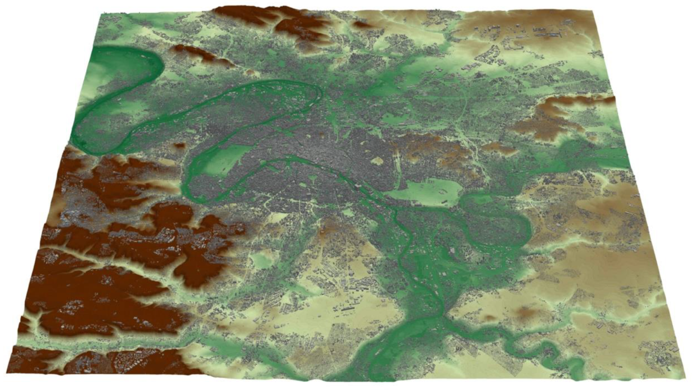
• 200 GB per timeframe for the domain covering Paris;
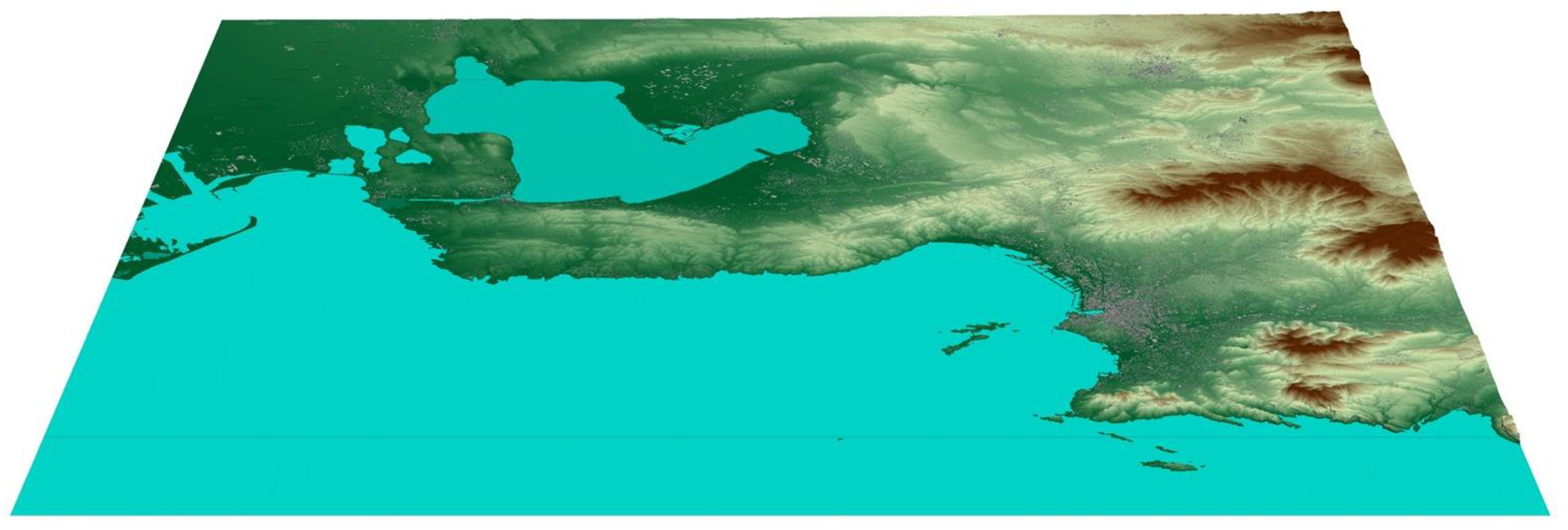
• 668 GB per timeframe for the domain covering Marseille.

These data do not interest directly the team handling the crisis management, with the exception maybe of the flow for the firefighters in the case of a fire associated with a release. Still, the modelers are required to inspect and verify the modeling of the flow and turbulence.

Regarding the transport and dispersion of the release, the size of the C data produced is directly proportional to:

• The area covered by the plume: the larger the plume, the larger the number of tiles that contain C data;
• The persistency duration of the plume in the domain;
• The averaging period used.

The area and persistency are strongly related to the transport and diffusion due to the flow.

Regarding the averaging period, since the transport and dispersion model is an LPDM, to compute a concentration field, particles have to be projected onto the computation grid. This is done during the averaging period. If the averaging period is 10 min, 6 values per grid point are obtained for one hour simulated. If this averaging period is 1 min, 60 values are obtained for one hour simulated. An averaging period of 10 min is sufficient for the needs of a crisis management team. As a modeler, it is nonetheless interesting to produce 1-min averages to obtain a more detailed view of the plume evolution, especially close to the source.

For the EMERGENCIES project, with 10 min averages, 90 GB of concentration data were produced to simulate a period of 5 h. This reaches 900 GB if 1-min averages are used.

For the EMED project, using 10 min averages, 85 GB of concentration data were produced to simulate a period of 4 h. This reaches 850 GB for 1-min averages.

The amount of data produced by the simulation ranges between around 100 GB and several TB. The fact that they were decomposed onto calculation tiles, and also the necessity for them to be rapidly and efficiently explored and manipulated in the context of crisis management led us to develop the approach presented in the following section.

3. Treatment and Visualization of the Data

After presenting the initial attempts for visualization, we introduce the methodology chosen based on multilevel tiled images. Then, we describe its implementation, with a particular focus on the treatment of vector field and the parallel distribution of calculations.

3.1. Initial Attemtps

With this large amount of data, the requirement is to be able to zoom in specific locations with a high level of details while at the same time being able to get a good understanding of what is occurring globally, with all this under the constraint of keeping a good level of interactivity.

In the EMERGENCIES project, the ability to produce any visualization of the results over the whole domain was not possible out of the box.

At first, parallel 3D scientific viewing was tried. The open-source data analysis and visualization application PARAVIEW [32] was selected due to its parallel capabilities. A dedicated plugin was developed. The plugin is relying on the computation tiles, i.e., the way the domain is decomposed by the PMSS modeling system: each tile is loaded by a PARAVIEW visualization server, and images can be generated in batch or through interactive views. Hence, the Paris domain required more than 1000 cores, one per PARAVIEW server, and the Marseille domain more than 2000 to operate the flow visualization. While the batch permitted to generate several views of interest (such as Figure 1, Figure 2 and Figure 3 above), through a lengthy iterative process of blind view setup then view production, it is not interactive. The interactive viewing was tested up to around 120 computation tiles, but it required several tens of second to change a point of view, which restricted its actual usability. It also required a large amount of core to be available at the exact time of the visualization, and during the whole visualization session.

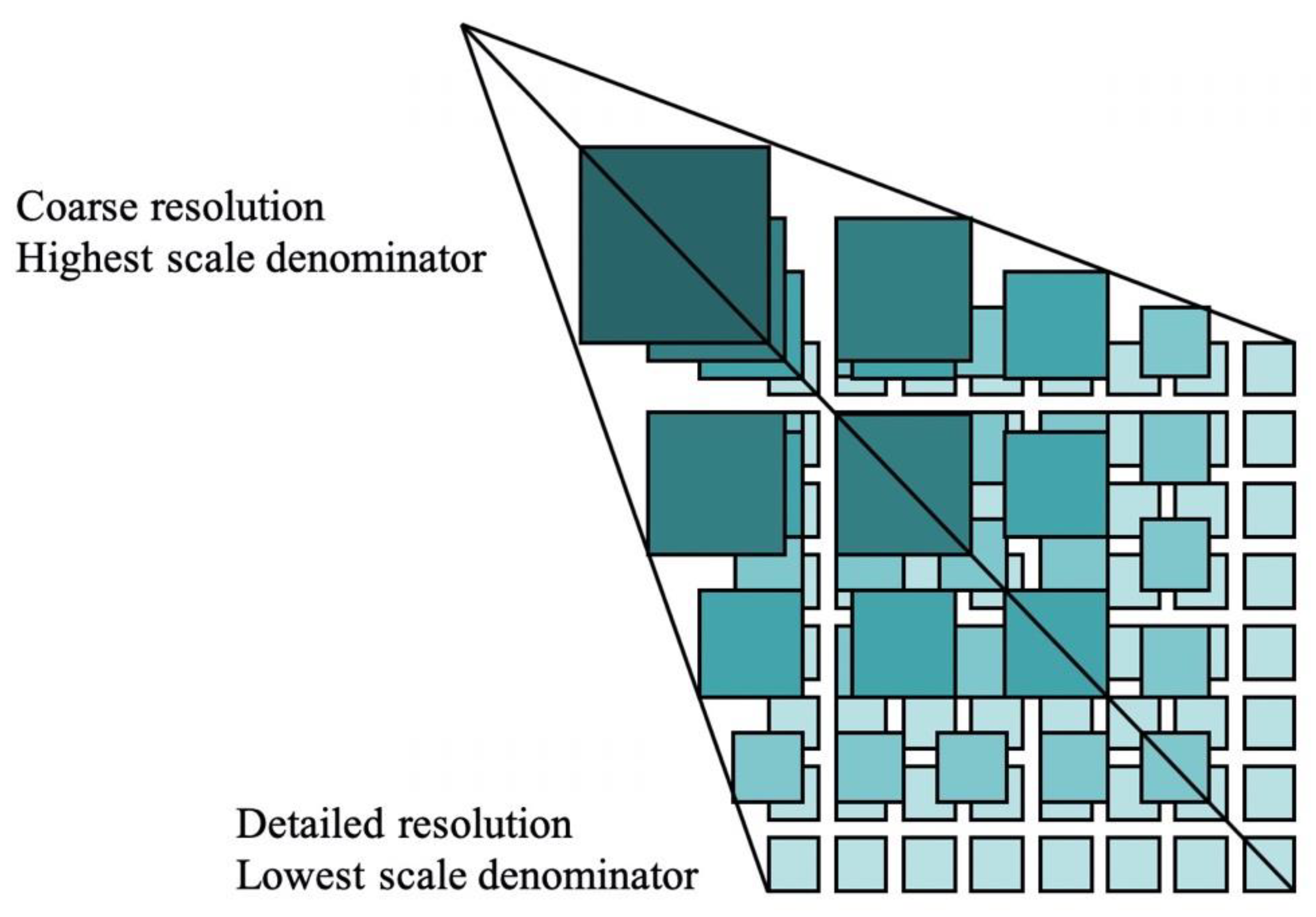
3.2. Introduction to the Methodology

The final methodology retained was taken from online cartography and very large high-resolution maps. The idea was to provide different levels of details at different zoom levels and to slice the data into visualization tiles at each level, as illustrated in Figure 4. The aim was to reduce the memory footprint of the data and limit it to the data being actually displayed in the view.

At each zoom level z, the global map for the Earth surface is divided in 2^z visualization tiles, and each tile has a size of 256 × 256 pixels, since each tile is an image, traditionally a portable network graphics (PNG) type. At each zoom level, the tiles are numbered according to their location along the west–east, the x coordinate, and north–south axis, the y coordinate.

From now on, each time we refer to a tile, it is a visualization tile. A tile related to the domain decomposition of the parallel scheme of the model is referred to as a computational tile.

We retained such approach since it enabled fast browsing through a cartographic-type client, while being able to display high level of details when required.

The treatment was performed directly on the computing cluster as a post-processing step performed on the FT or C simulation data. The tiles were then made available through a web server and displayed by a JavaScript client on any web browser.

The post-processing was performed on a set of FT or C data, for a set of time frames and vertical levels. Accessing the actual values of each field, instead of producing a colored image, was required to be able to change the coloring scale or explore vector outputs such as the flow field. Hence, floats were encoded in 4 bytes and stored directly in the PNG files by using the 4 bytes normally distributed to the red, green, blue, and alpha channels.

3.3. Details on the Multilevel Tiling Implementation

The post-processing was performed in parallel using the message passing interface (MPI) standard. After describing the algorithm, we discuss the particular of vector fields such as the wind flow.

3.3.1. Parallel Scheme

The scheme relied on the Tiff file standard [33] and the Geospatial Data Abstraction Library (GDAL) [34]. It used the Tiff virtual stack approach to handle the domain decomposition inherited from the parallel calculation and see the group of Tiff files generated from each calculation tile as multiple parts of a single large Tiff file. It went through the following steps:

• First step, generation of the Tiff files:

  ○

  Distribution of the analysis of available bin files to available cores to retrieve available fields, domain coordinates, available time steps;

  ○

  Calculation by the master core of the large domain footprint, the tiles coordinates required for each zoom levels and the time steps to extract;

  ○

  Generation of Tiff files for each FT or C data file, and for each vertical level and time step selected. The files are generated using the Google Mercator projection;

  ○

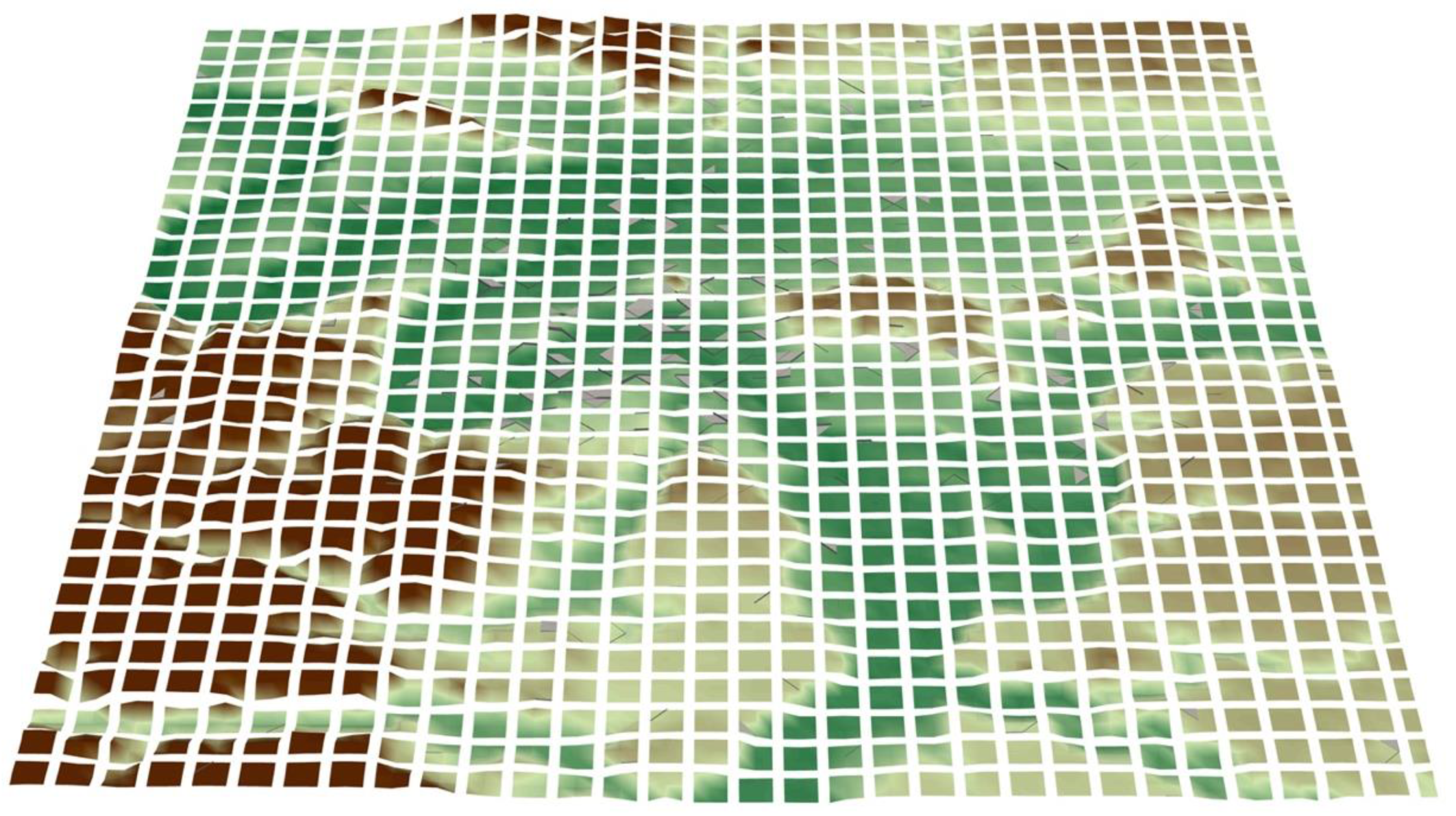
  Creation of a Tiff virtual stack encompassing the whole calculation domain, the domain being, or not, decomposed in multiple computation tiles of arbitrary dimension;

• Second step, generation of the tiles from the Tiff files:

  ○

  Loop on zoom levels being treated starting from the larger zoom level;

  ○

  Distribution of each tile, from the total pool of tiles combining field name, time step and vertical level, to a core for generation.

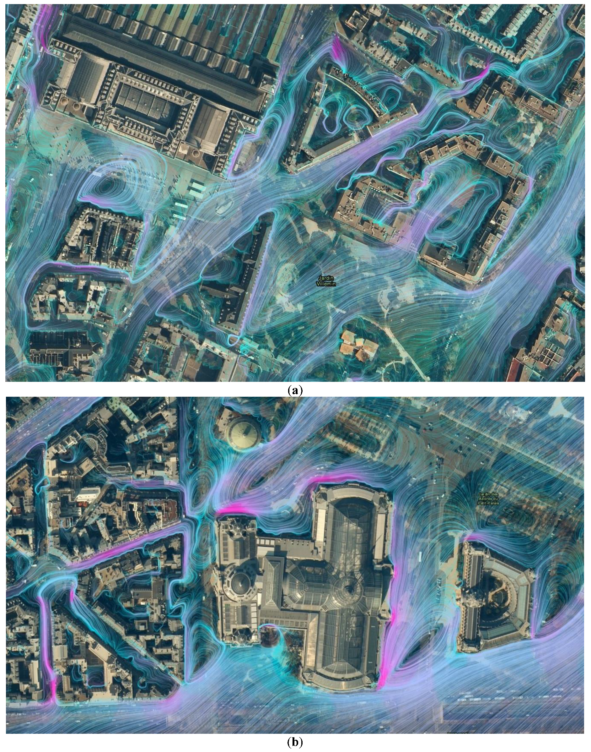
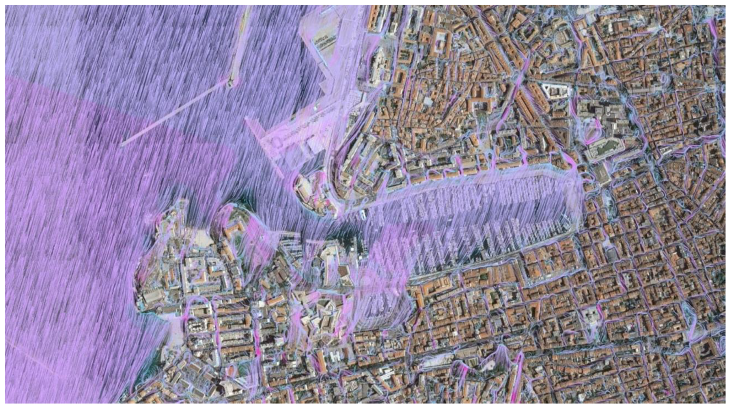
3.3.2. Specificity for Vector Fields

For the vector fields visualization, additional treatment was performed but only on the client side. Indeed, the methodology for the post-processing was similar to the one used for a scalar field, with each component of the vector field being generated as a scalar field.

The visualization client then treated specifically the vector field by proposing either to view each component individually or by treating them as a vector field and offering streamline visualization. Streamlines were generated by using visualization particles which trajectories of are drawn on the screen. Visualization particles were exchanged between tiles to prevent streamline boundaries to appear at each tile boundary.

A dedicated presentation of the client will be available in a future publication.

4. Results

After presenting the results obtained for the EMERGENCIES and EMED data, we describe the performances of this approach then discuss its usability in crisis management.

4.1. Visualization

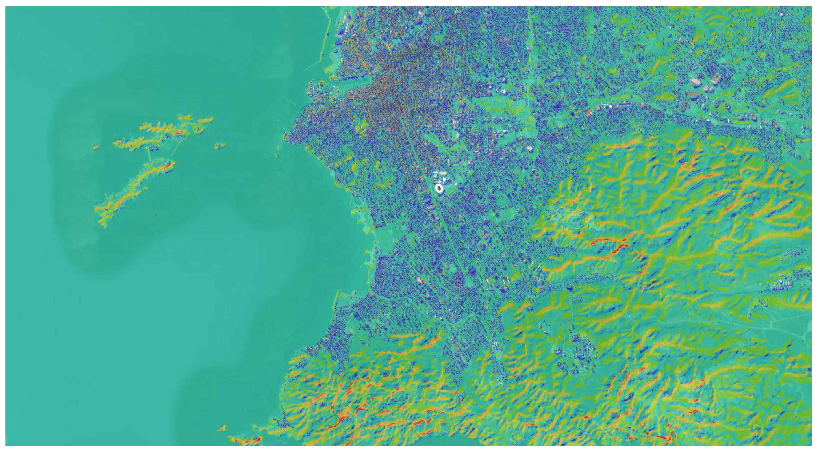
4.1.1. Flow and Turbulence Data

As described above, the flow was computed by the PMSS modeling system with a grid step of 3 m: A detailed view of the flow is presented in Figure 5 close to the train station and the museum of the project EMERGENCIES. The streamlines reveal the details of the flow and its importance for the dispersion pattern close to the source, especially regarding the entrapment of the concentration obviously in the buildings, but also in the recirculation zones and some narrow canyon streets nearby.

This type of analysis is particularly important for the modeler to evaluate the quality of the modeling and attain an understanding on the concentration patterns computed by the model.

The capability to visualize the flow streamlines on a large area is displayed in Figure 6. The flow can hence be visualized on a large area to understand the global flow pattern, while specific analysis at the scale of the road or the building is also available in any locations of these very large domains.

Obviously, the wind speed can also be presented. Figure 7 displays the wind speed in the Marseille city center and on the topography south of the city.

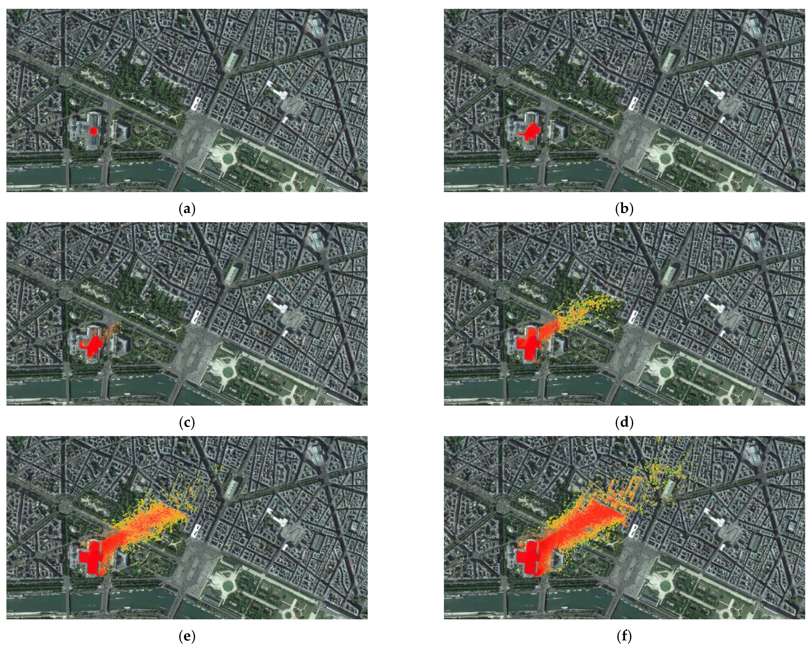
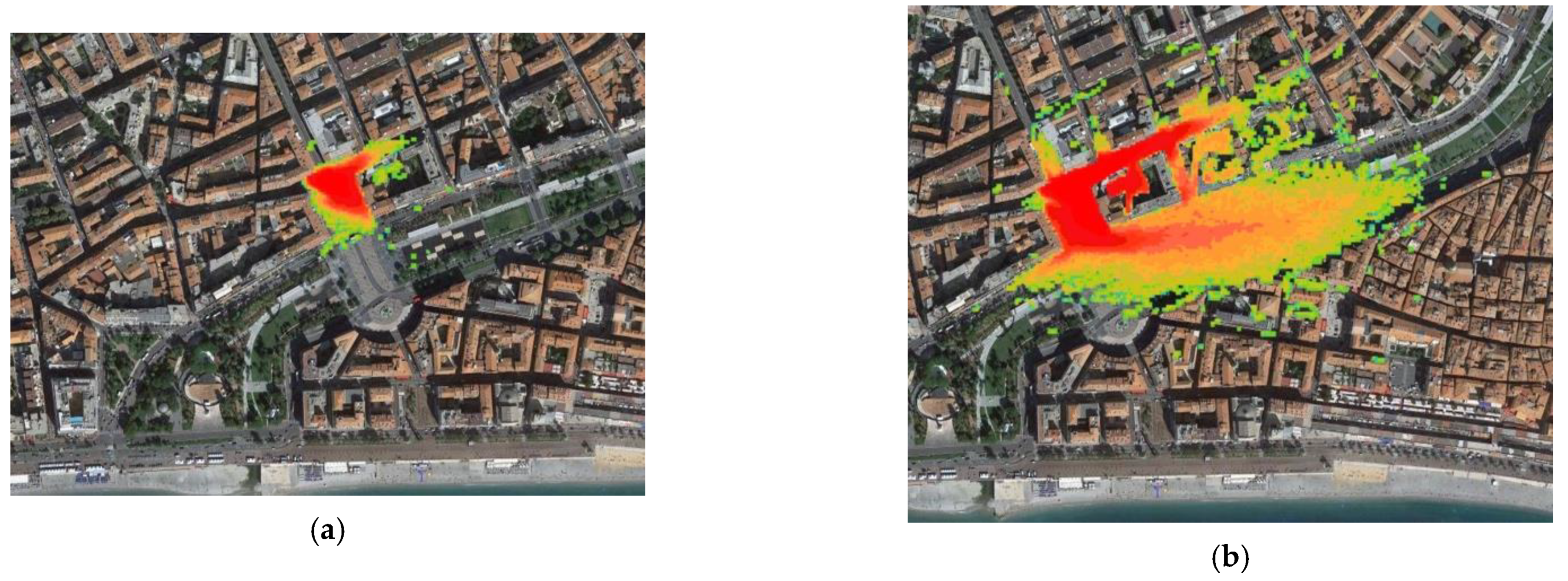
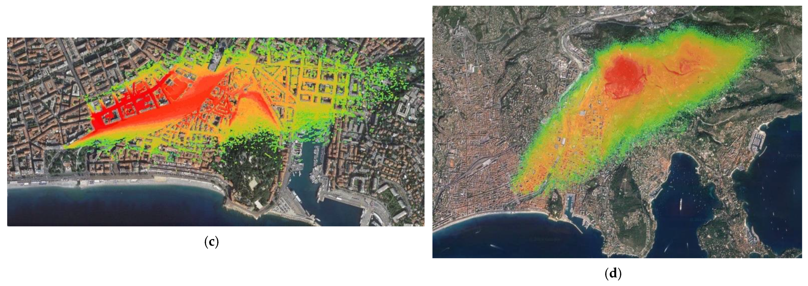
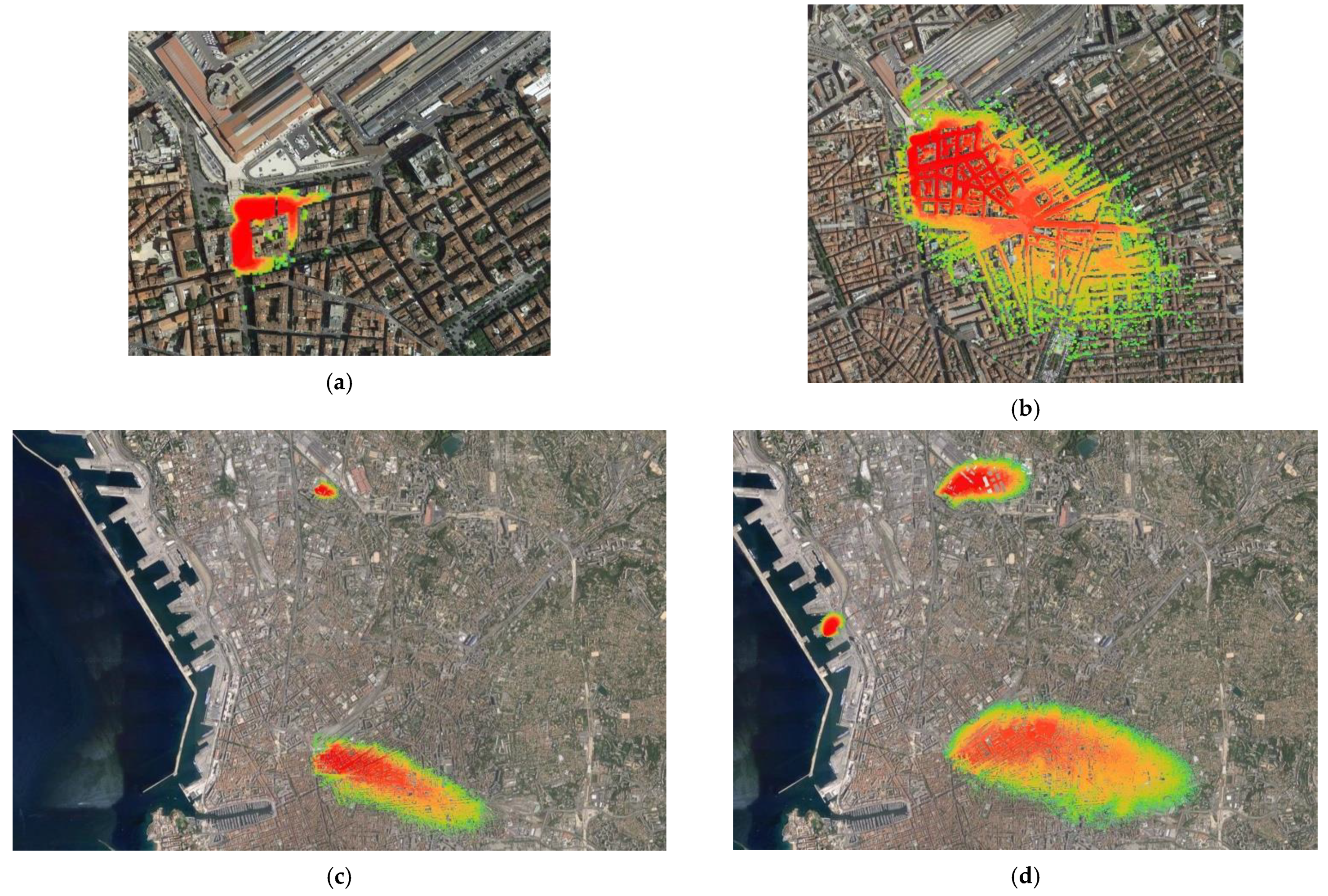
4.1.2. Concentration Data

The concentration field of the EMERGENCIES project for the first minutes after the release inside the museum is presented on Figure 8. It shows the dispersion pattern first within the building (Figure 8a–c), then in the rather open field close to the museum (Figure 8d,e), and finally in the streets to the north (Figure 8f).

The release in the city of Nice in the EMED is displayed in Figure 9. The release occurred in a plaza, the Place Massena, (Figure 9a) and the plume was both trapped in the plaza and transported rapidly by the stronger flow in the large street south of the release (Figure 9b). It then hit a first hill, the Colline du Chateau (Figure 9c), before moving away and reaching the strong mountainous topography northeast of Nice, while remaining trapped in some narrow streets of the city center (Figure 9d).

In Figure 10, for the multiple releases in the Marseille domain, various zoom levels allowed the global pattern of the plume to be displayed while being able to also focus on pollutant entrapment inside canyon streets.

4.2. Performances

Performances of the methodology were evaluated both regarding the post-processing prior to the navigation, but also obviously during the navigation.

4.2.1. Post-processing Step

Performances of the creation of the multilevel tiled data were also relevant since they had to be included in the duration of the simulation, especially for a modeling system aimed at crisis management.

The parallel scheme had very limited communications between cores but was limited by the number of tiles that could be distributed among cores. Still, the fewer the tiles, the smaller the domain size and the lower the computational cost of the post-processing step.

The post-processing step had been performed on the same infrastructure as the simulations for the projects.

Regarding the flow and turbulence treatment, the zoom level was constructed between the levels 10 and 16. The levels above 16 were useless since the grid size of the mesh for the modeling system was 3 m, and at zoom level 16, the pixel size on the equator was below 3 m.

For the wind flow field, either in the Paris or Marseille domains, the treatment per timeframe using 100 cores required less than 10 min.

For the concentration data at 1 min, and since the data were stored in a single file per tile for the whole duration of the simulation, the treatment for the whole period of time used 50 cores and required roughly 2 h either for Marseille or Paris. For the Marseille domain, the simulation duration was 4 h and the binaries contained 240 timeframes; hence, the post-processing required 30 s on average per timeframe.

Regarding the disk size, the data produced for exploration had sizes similar to the raw binary output of the model, being binary too, with a maximum zoom level, 16, which led to a pixel size being of the same order of magnitude as the grid size of the model. A small overhead was due to the size of the additional zoom level above 16. On the other side, not all the vertical levels were extracted but mainly the levels near the ground.

As an illustration, the EMED concentration data, using 10-min averages for the concentration, had a size of 85 GB, while the multilevel tiles limited to the first two vertical levels had a size of 3.2 GB.

4.2.2. Navigation

The navigation through the data was limited by the capability of the server serving the tiles to support a defined level of workload. This being a problem of server scalability, which is rarely an issue in the context of crisis management where the number of team members accessing the data is very limited, the visualization on the client side was similar with the experience of a user browsing through any web mapping service:

• Data are accessible in less than several seconds, whatever the global size of the domain;
• Change in locations used the tiling capability, with additional tiles being loaded when required;
• Change in zoom allows both large scale and small-scale features to be monitored.

4.3. Discussion for Crisis Management

The approach taken here allowed us to:

• Take the most out of the computing infrastructure during the modeling phase by preparing the output;
• Enable a very efficient navigation in and consultation of the result during the exploitation of the simulation, even for non-expert users of modeling due to the very large diffusion of web mapping tools.

The web mapping approach allows a better integration of the simulation results in third parties integration tools, especially geographical information systems (GIS), which have increasing availability during crisis management.

It also allows the modeler to explore the results even for very large simulation results like the flow data presented above.

5. Conclusions

The EMERGENCIES and EMED project demonstrated the operational capability of high-resolution modeling in built-up areas for crisis management and supported by high-performance computing. These projects pointed out the vital importance of a capability to visualize easily and in time compatible with emergency situations the simulation results.

Since these projects were applied on responsibility areas of actual emergency teams, they generated very large amounts of data that made it all the more difficult to explore the data generated.

While an initial approach relying on traditional 3D scientific viewing permitted us to create visualizations in batch mode for such large results, this approach proved to be difficult to use as an actual operational capability. This was mainly related to limits in interactivity.

An alternative approach was introduced taken from the field of web mapping by using multilevel tiled images. The approach was implemented in a parallel library to be used as a post-processing step after the simulation of the flow and the dispersion and on the same infrastructure. The approach was also modified to allow us to display values rather than images, time-dependent and multi-height results, and scalar or vector fields.

The performance of the parallel post-processing step proved to be largely compatible with the requirement of the emergency situation, since the intensity in calculation and time required were significantly lower than those of the simulation in itself.

The actual navigation in the result either by the emergency team or the modeler was similar with the one experienced by any web mapping tool user, and hence very satisfactory to the requirement in terms of rapidity and capability do visualize both the larger scale but also the fine details.

This kind of tool is also widely known among the users, and it has natural integration capabilities in third party tools such as GIS.

This approach is hence of paramount importance for the adoption of high-resolution modeling in built-up areas by the crisis management teams, either during preparation of exercises or during an actual situation management.

In a context of increasing adoption of virtual or augmented reality (AR/VR) tools in the crisis management community, proving again the vital importance of very efficient visualization tools for the simulation community, additional perspectives are under studies to allow the integration of modeling results in the framework of AR/VR.

References

1. Armand, P.; Bartzis, J.; Baumann-Stanzer, K.; Bemporad, E.; Evertz, S.; Gariazzo, C.; Gerbec, M.; Herring, S.; Karppinen, A.; Lacome, J.M.; et al. Trini Castelli S (2015) Best practice guidelines for the use of the atmospheric dispersion models in emergency response tools at local-scale in case of hazmat releases into the air. Tech Rep, COST Action ES 1006. Available online: http://elizas.eu/images/Documents/Best%20Practice%20Guidelines_web.pdf (accessed on 16 July 2021).
2. Biltoft, C.A. Customer Report for Mock Urban Setting Test; DPG Document Number 8-CO-160-000-052; Defense Threat Reduction Agency: Alexandria, VA, USA, 2001.
3. Warner, S.; Platt, N.; Heagy, J.F.; Jordan, J.E.; Bieberbach, G. Comparisons of transport and dispersion model predictions of the mock urban setting test field experiment. J. Appl. Meteorol. Climatol. 2006, 45, 1414–1428. [Google Scholar] [CrossRef]
4. Allwine, K.J.; Flaherty, J. Joint Urban 2003: Study Overview and Instrument Locations; PNNL-15967; Pacific Northwest National Lab.: Richland, WA, USA, 2006. [Google Scholar]
5. Hernández-Ceballos, M.A.; Hanna, S.; Bianconi, R.; Bellasio, R.; Mazzola, T.; Chang, J.; Andronopoulos, S.; Armand, P.; Benbouta, N.; Čarný, P.; et al. UDINEE: Evaluation of multiple models with data from the JU2003 puff releases in Oklahoma City. Part I: Comparison of observed and predicted concentrations. Bound. Layer Meteorol. 2019, 171, 323–349. [Google Scholar] [CrossRef]
6. Hernández-Ceballos, M.A.; Hanna, S.; Bianconi, R.; Bellasio, R.; Chang, J.; Mazzola, T.; Andronopoulos, S.; Armand, P.; Benbouta, N.; Čarný, P.; et al. UDINEE: Evaluation of multiple models with data from the JU2003 puff releases in Oklahoma City. Part II: Simulation of puff parameters. Bound. Layer Meteorol. 2019, 171, 351–376. [Google Scholar] [CrossRef]
7. EPA; NOAA. Area Locations of Hazardous Atmospheres (ALOHA); User’s Manual; US Environmental Protection Agency (USEPA) and the National Oceanic and Atmospheric Administration (NOAA): Washington, DC, USA, 1999.
8. Sykes, R.I.; Parker, S.F.; Henn, D.S.; Cerasoli, C.P.; Santos, L.P. PC-SCIPUFF Version 1.3 Technical Documentation; ARAP Report No. 725; Titan Corporation, ARAP Group: Princeton, NJ, USA, 2000. [Google Scholar]
9. Chang, J.C.; Hanna, S.R.; Boybeyi, Z.; Franz, P. Use of Salt Lake City URBAN 2000 field data to evaluate the urban hazard prediction assessment capability (HPAC) dispersion model. J. Appl. Meteorol. 2005, 44, 485–501. [Google Scholar] [CrossRef]
10. Milliez, M.; Carissimo, B. Numerical simulations of pollutant dispersion in an idealized urban area. for different meteorological conditions. Bound. Layer Meteorol. 2007, 122, 321–342. [Google Scholar] [CrossRef]
11. Gowardhan, A.A.; Pardyjak, E.R.; Senocak, I.; Brown, M.J. A CFD-based wind solver for urban response transport and dis-persion model. Environ. Fluid Mech. 2011, 11, 439–464. [Google Scholar] [CrossRef]
12. Yee, E.; Lien, F.S.; Ji, H. A Building-Resolved Wind Field Library for Vancouver: Facilitating CBRN Emergency Response for the 2010 Winter Olympic Games; Defense Research and Development: Suffield, AB, Canada, 2010. [Google Scholar]
13. Armand, P.; Christophe, D.; Luc, P. Is it now possible to use advanced dispersion modelling for emergency response? The example of a CBRN-E exercise in Paris. In Air Pollution Modeling and its Application XXIV; Springer: Cham, Switzerland, 2016; pp. 433–446. [Google Scholar]
14. Oldrini, O.; Armand, P.; Duchenne, C.; Perdriel, S.; Nibart, M. Accelerated Time and High-Resolution 3D Modeling of the Flow and Dispersion of Noxious Substances over a Gigantic Urban Area—The EMERGENCIES Project. Atmosphere 2021, 12, 640. [Google Scholar] [CrossRef]
15. Armand, P.; Duchenne, C.; Oldrini, O.; Perdriel, S. Emergencies Mediterranean—A Prospective High-Resolution Modelling and Decision-Support System in Case of Adverse Atmospheric Releases Applied to the French Mediterranean Coast. In Proceedings of the 18th International Conference on Harmonisation within Atmospheric Dispersion Modeling for Regulatory Purposes, Bologna, Italy, 9–12 October 2017; pp. 9–12. [Google Scholar]
16. OSGEO. Tile Map Service Specification. Available online: https://wiki.osgeo.org/wiki/Tile_Map_Service_Specification (accessed on 16 July 2021).
17. Oldrini, O.; Olry, C.; Moussafir, J.; Armand, P.; Duchenne, C. Development of PMSS, the Parallel Version of Micro SWIFT SPRAY. In Proceedings of the 14th International Conference on Harmonisation within Atmospheric Dispersion Modelling for Regulatory Purposes, Kos, Greece, 2–6 October 2011; pp. 443–447. [Google Scholar]
18. Oldrini, O.; Armand, P.; Duchenne, C.; Olry, C.; Tinarelli, G. Description and preliminary validation of the PMSS fast response parallel atmospheric flow and dispersion solver in complex built-up areas. J. Environ. Fluid Mech. 2017, 17, 1–18. [Google Scholar] [CrossRef]
19. Oldrini, O.; Armand, P.; Duchenne, C.; Perdriel, S. Parallelization Performances of PMSS Flow and Dispersion Modelling System over a Huge Urban Area. Atmosphere 2019, 10, 404. [Google Scholar] [CrossRef] [Green Version]
20. Oldrini, O.; Armand, P. Validation and sensitivity study of the PMSS modelling system for puff releases in the Joint Urban 2003 field experiment. Bound. Layer Meteorol. 2019, 171, 513–535. [Google Scholar] [CrossRef]
21. Moussafir, J.; Oldrini, O.; Tinarelli, G.; Sontowski, J.; Dougherty, C. A new operational approach to deal with dispersion around obstacles: The MSS (Micro-Swift-Spray) software suite. In Proceedings of the 9th International Conference on Harmonisation within Atmospheric Dispersion Modelling for Regulatory Purposes, Garmisch-Partenkirchen, Germany, 1–4 June 2004; Volume 2, pp. 114–118. [Google Scholar]
22. Tinarelli, G.; Brusasca, G.; Oldrini, O.; Anfossi, D.; Trini Castelli, S.; Moussafir, J. Micro-Swift-Spray (MSS) a new modelling system for the simulation of dispersion at microscale. General description and validation. In Air Pollution Modelling and Its Applications XVII; Borrego, C., Norman, A.N., Eds.; Springer: Boston, MA, USA, 2007; pp. 449–458. [Google Scholar]
23. Oldrini, O.; Nibart, M.; Armand, P.; Olry, C.; Moussafir, J.; Albergel, A. Introduction of Momentum Equations in Mi- cro-SWIFT. In Proceedings of the 15th International Conference on Harmonisation within Atmospheric Dispersion Modelling for Regulatory Purposes, Varna, Bulgaria, 8–11 September 2014. [Google Scholar]
24. Oldrini, O.; Nibart, M.; Duchenne, C.; Armand, P.; Moussafir, J. Development of the parallel version of a CFD–RANS flow model adapted to the fast response in built-up environments. In Proceedings of the 17th International Conference on Harmonisation within Atmospheric Dispersion Modelling for Regulatory Purposes, Budapest, Hungary, 9–12 May 2016. [Google Scholar]
25. Röckle, R. Bestimmung der Strömungsverhaltnisse im Bereich Komplexer Bebauungs-Strukturen. Doctoral Thesis, Technical University Darmstadt, Darmstadt, Germany, 1990. [Google Scholar]
26. Anfossi, D.; Desiato, F.; Tinarelli, G.; Brusasca, G.; Ferrero, E.; Sacchetti, D. TRANSALP 1989 experimental campaign—II. Simulation of a tracer experiment with Lagrangian particle models. Atmos. Environ. 1998, 32, 1157–1166. [Google Scholar] [CrossRef]
27. Tinarelli, G.; Mortarini, L.; Trini Castelli, S.; Carlino, G.; Moussafir, J.; Olry, C.; Armand, P.; Anfossi, D. Review and validation of Micro-Spray, a Lagrangian particle model of turbulent dispersion. In Lagrangian Modelling of the Atmosphere, Geophysical Monograph; American Geophysical Union (AGU): Washington, DC, USA, May 2013; Volume 200, pp. 311–327. [Google Scholar]
28. Rodean, H.C. Stochastic Lagrangian Models of Turbulent Diffusion; American Meteorological Society: Boston, MA, USA, 1996; Volume 45. [Google Scholar]
29. Thomson, D.J. Criteria for the selection of stochastic models of particle trajectories in turbulent flows. J. Fluid Mech. 1987, 180, 529–556. [Google Scholar] [CrossRef]
30. Archambeau, F.; Méchitoua, N.; Sakiz, M. Code Saturne: A finite volume code for the computation of turbulent incompressible flows-Industrial applications—Industrial Applications. Int. J. Finite Vol. 2004, 1, 1. [Google Scholar]
31. Skamarock, W.C.; Klemp, J.B.; Dudhia, J.; Gill, D.O.; Barker, D.M.; Duda, M.G.; Huang, X.-Y.; Wang, W.; Powers, J.G. 2008: A Description of the Advanced Research WRF Version 3; NCAR Tech. Note NCAR/TN-475+STR; UCAR Communications: Boulder, CO, USA, 2008. [Google Scholar] [CrossRef]
32. Ahrens, J.; Geveci, B.; Law, C. ParaView: An End-User Tool for Large Data Visualization; Visualization Handbook; Elsevier: Amsterdam, The Netherlands, 2005; ISBN 978-0123875822. [Google Scholar]
33. Adobe Developers Association. TIFF” Revision 6.0, Jun. 3, 1992; Adobe Systems Incorporated: Mountain View, CA, USA, 1992. [Google Scholar]
34. Warmerdam, F. The geospatial data abstraction library. In Open Source Approaches in Spatial Data Handling; Springer: Berlin/Heidelberg, Germany, 2008; pp. 87–104. [Google Scholar]
Figure 1. 3D view of the topography and buildings. North is at the top.
Atmosphere 12 00920 g001
Figure 2. Domain decomposition of the domain in 1088 tiles.
Atmosphere 12 00920 g002
Figure 3. 3D view of the topography and buildings for the Marseille domain. North is at the top.
Atmosphere 12 00920 g003
Figure 4. Multi-level tiled, or pyramidal, image (Copyright 2019 Open Geospatial Consortium).
Atmosphere 12 00920 g004
Figure 5. Closeup view of the flow streamlines computed in the streets near (a) the train station and (b) the museum. North is at the top.
Atmosphere 12 00920 g005
Figure 6. View of the flow streamlines computed in the Vieux Port area in Marseille. North is at the top.
Atmosphere 12 00920 g006
Figure 7. View of the wind speed in the Marseille city center and on the topography south of the city. North is at the top.
Atmosphere 12 00920 g007
Figure 8. View, for the EMERGENCIES project, of the plume inside and in the vicinity of the museum: (a) 1 min after the release; (b) 3 min; (c) 4 min; (d) 6 min; (e) 8 min; (f) 10 min. The change from the 1-m resolution of the inner domain to the 3-m resolution of the large domain can be noticed. The threshold for 500 µg/m3 of concentration is in red, while that for 1 µg/m3 is in orange and that for 0.001 µg/m3 is in green. North is at the top.
Atmosphere 12 00920 g008
Figure 9. View, for the EMED project and the release in the Nice domain, of the plume in the vicinity and further away from the release: (a) 2 min after the release; (b) 5 min; (c) 15 min; (d) 55 min. The scale, and the zoom level, vary between the views to cope with the evolution of the plume. The threshold for 500 µg/m3 of concentration is in red, while that for 1 µg/m3 is in orange and that for 0.01 µg/m3 is in green. North is at the top.
Atmosphere 12 00920 g009aAtmosphere 12 00920 g009b
Figure 10. View, for the EMED project and the release in the Marseille domain, of the three plumes in the vicinity and further away from the releases: (a) 3 min after the first release; (b) 15 min; (c) 38 min; (d) 75 min. The scale, and the zoom level, vary between the views to cope with the evolution of the plumes. The threshold for 500 µg/m3 of concentration is in red, while that for 1 µg/m3 is in orange and that for 0.01 µg/m3 is in green. North is at the top.
Atmosphere 12 00920 g010
Publisher’s Note: MDPI stays neutral with regard to jurisdictional claims in published maps and institutional affiliations.