Toward Development of a Framework for Prediction System of Local-Scale Atmospheric Dispersion Based on a Coupling of LES-Database and On-Site Meteorological Observation

Abstract

An accurate analysis of local-scale atmospheric dispersion of radioactive materials is important for safety and consequence assessments and emergency responses to accidental release from nuclear facilities. It is necessary to predict the three-dimensional distribution of the plume in consideration of turbulent effects induced by individual buildings and meteorological conditions. In this study, first, we conducted with meteorological observations by a Doppler LiDAR and simple plume release experiments by a mist-spraying system at the site of Japan Atomic Energy Agency. Then, we developed a framework for prediction system of local-scale atmospheric dispersion based on a coupling of large-eddy simulation (LES) database and on-site meteorological observation. The LES-database was also created by pre-calculating high-resolution turbulent flows in the target site at mean wind directions of class interval 10°. We provided the meteorological observed data with the LES-database in consideration of building conditions and calculated the three-dimensional distribution of the plume with a Lagrangian dispersion model. Compared to the instantaneous shots of the plume taken by a digital camera, it was shown that the mist plume transport direction was accurately simulated. It was concluded that our proposed framework for prediction system based on a coupling of LES-database and on-site meteorological observation is effective.

1. Introduction

In an emergency response to accidental release of radioactive materials from nuclear facilities on a local-scale, it is important to accurately and quickly predict the air concentrations at the evaluation point for internal doses and surface concentrations for external doses to evaluate the radiological consequences in consideration of the influence of turbulent effects induced by individual buildings and meteorological disturbances. For investigating plume dispersion over complex surface geometry in distances of up to several kilometers from the emission source, computational fluid dynamics (CFD) models are useful.

In principle, there are two approaches in CFD models: Reynolds-Averaged Navier–Stokes (RANS) and Large-Eddy Simulation (LES) models. RANS-based CFD models calculate a mean wind flow to deliver an ensemble- or time-averaged solution, and all turbulent motions are modeled using turbulence parameterization. The main advantage of the RANS model is its efficiency in simulating a mean flow field at a relatively low computational cost. However, it was reported that lateral dispersion behaviors of a plume are not reproduced well [1,2,3]. Recently, LES-based CFD models have also become useful tools. The basic idea of LES models resolves grid-scale turbulent motions and parameterizes only subgrid-scale motions. The advantage is that they can well capture plume dispersion behaviors in complex turbulent flows such as impinging, separated, and recirculating flows around buildings [2,3,4,5,6,7]. However, LES models also have a significant disadvantage of calculation time for emergency response purposes. To solve the trade-off problem of calculation time and prediction accuracy, we developed a combined LES-database/RANS model in which dispersion fields are simulated by RANS with LES pre-calculated wind velocity data and applied to plume dispersion in an actual urban central district [8]. It was shown that the combined model accurately reproduces horizontal concentration distributions obtained from a wind tunnel experiment for a simple street canyon case [5]. In addition, for a real urban area case, it was found that the results of the combined model reasonably agree with those of the LES used alone, although the underestimation in low concentration areas was observed. We concluded from these results that the combined model provides accurate results with a reasonable calculation time 1/40 times shorter than the LES model alone. However, this model evaluation was conducted under an ideal atmospheric condition in which the mean wind speeds and directions are constant. An important issue was remained in incorporating meteorological information into the model as input conditions.

Collier et al. [9] developed an operational dispersion model known as the Nuclear Accident Model (NAME) by combining with meteorological observations (OBS). The NAME model was designed based on a Lagrangian particle model and two mobile Doppler LiDAR systems. The dispersion processes of large numbers of imaginary particles are calculated by the mean flow and the turbulence parameters obtained from the dual-Doppler LiDAR dataset. The NAME is used for many applications such as nuclear accidents, pollutant episode studies, source term estimation, and air quality forecasting over a wide region of several 100 km². Recently, the on-site measurement coupled to CFD approach has been applied to wind resource assessment by several researchers [10,11,12]. For example, Radunz et al. [12] developed a framework based on a combination of on-site OBS and CFD and showed a fast and comprehensive solution to produce a wind resource map and estimate energy yield over a wide region of 144 km² by prescribing accurate CFD inflow conditions obtained from on-site OBS. These studies indicate the usefulness of a coupling of on-site OBS and CFD.

In the case of nuclear accidents, radioactive materials are assumed to be released into the atmosphere directly from a nuclear reactor building rather than an exhaust stack in many cases. In such a situation, plume transport and dispersion are highly influenced by individual buildings and structures, which results in inhomogeneous distributions of air concentrations. In this study, we propose a framework for prediction system of local-scale atmospheric dispersion based on a coupling of LES-database and on-site OBS that takes into account both individual buildings and real meteorological conditions. Toward development of the framework, first, we performed LESs of turbulent flows over a target site and created the dataset of mean and turbulent flows for 36 mean wind directions at 10° class interval. Then, we conducted with meteorological observations by a Doppler LiDAR and simple dispersion experiments using a mist-spraying system for representing a plume at the site of Japan Atomic Energy Agency (JAEA). Here, the dispersion behaviors of the water mist plume were observed using a digital camera. Our objective is to investigate the effectiveness of the coupling of the LES-database and on-site OBS by comparing the coupling simulation results with the transport direction of the water mist plume.

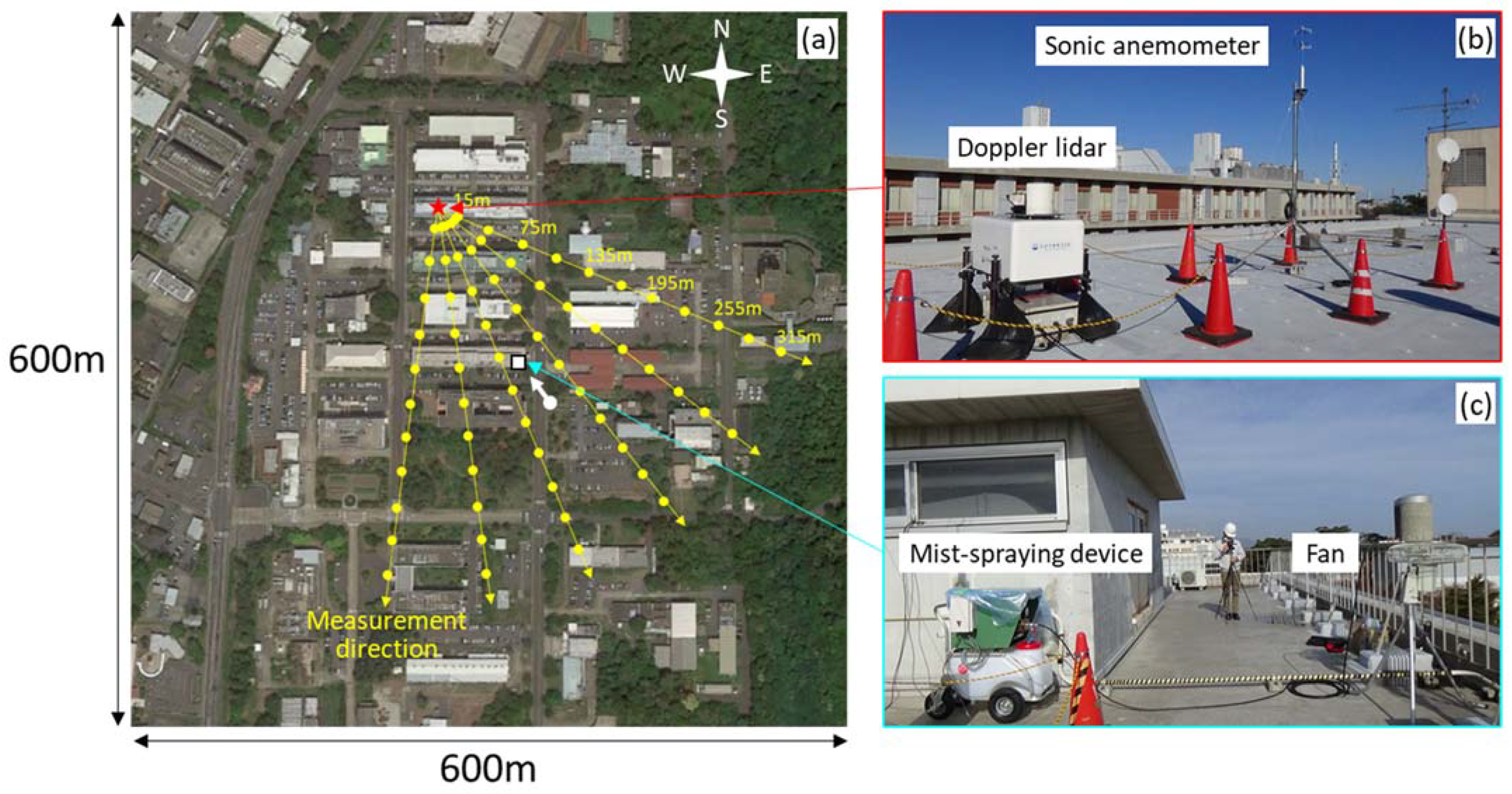
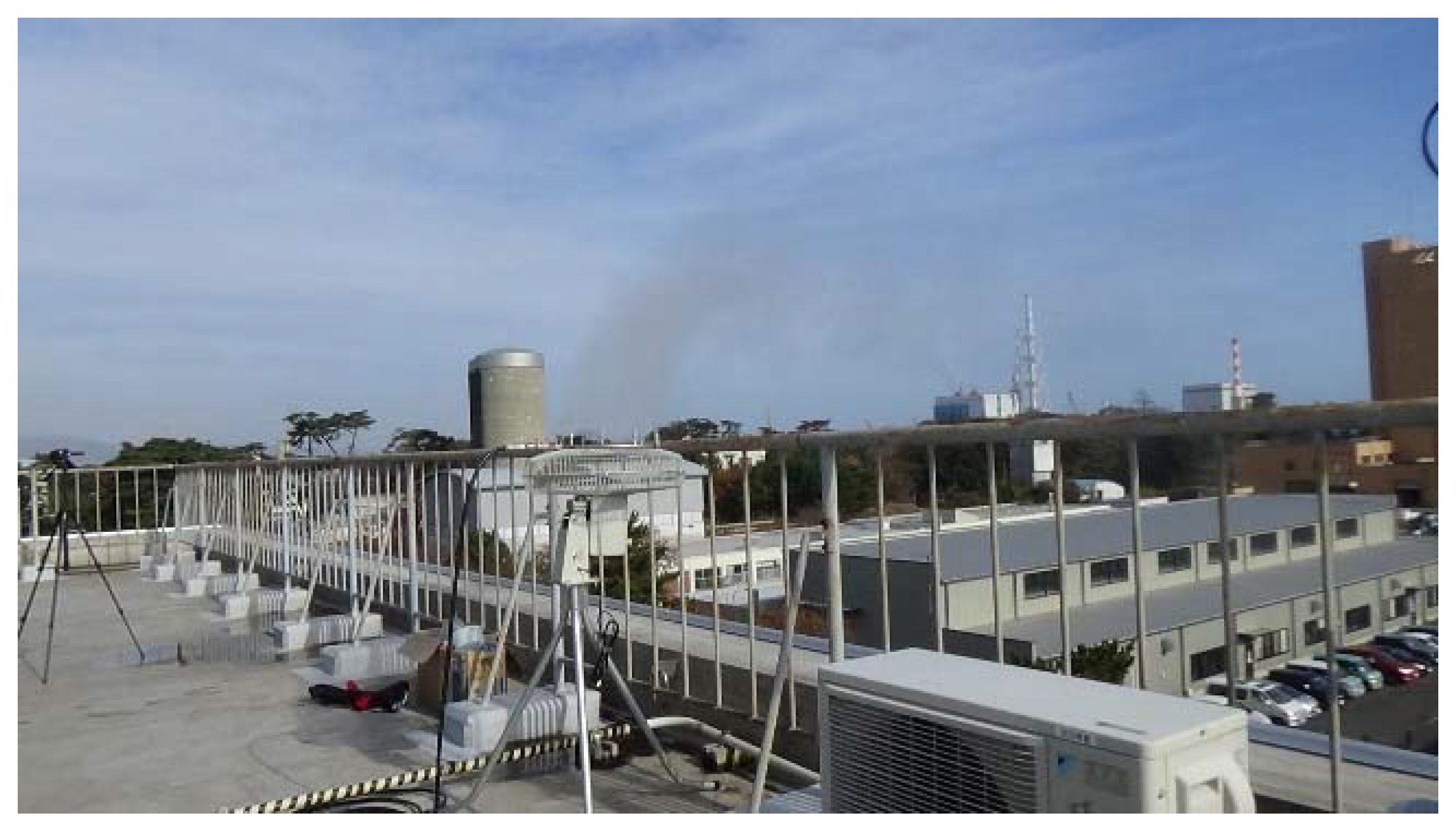
2. Field Experiments

Meteorological observations were conducted at the site of JAEA Nuclear Science Research Institute (NSRI), Tokai-mura, Ibaraki prefecture, Japan during the period from 16 November to 23 December 2020. A mist plume was continuously released by a mist-spraying system for 10 min several times during the period from 1049 JST to 1132 JST 26 November and from 1030 JST to 1122 JST 1 December. The target site and the locations of the experimental devices are shown in Figure 1. A Doppler LiDAR (Streamline Pro, HALO Photonics Ltd.) and an ultrasonic anemometer (WindMaster II, Gill Instruments Ltd.) were placed on the building rooftop at 12-m height. The laser beam was intensively directed toward the position of the mist-spraying system. The Doppler LiDAR repeatedly conducted a 3-min scan sequence, which included four Plan Position Indicator (PPI) scans at elevation angles of 1.0°, 7.6°, 14.9° and 21.8°, and six Range Height Indicator (RHI) scans at azimuth angles with a 15° interval. The detection range was from 15 m to 3000 m, with a range resolution of 35 m in the radial direction. However, the missing rate of the Doppler LiDAR was extremely high at the positions 300 m away from there. Nakano et al. [13] measured wind direction and velocity data by a Doppler LiDAR (Windcube WLS7, Leosphere Ltd.) at the site located approximately 2 km south of the NSRI of JAEA for one-year starting from 1st February 2012 and showed that the missing rate of the Doppler LiDAR was high especially during the period from late autumn to winter. The tendency of the high missing rate during our observation period is the same as their one-year observation [13]. Figure 2 shows an example of spatial distributions of the observed radial wind speeds at elevation angles of 1.0°, 7.6°, 14.9°, and 21.8°. Those were linearly interpolated on grids of 1 m × 1 m in the horizontal direction and were used for plume dispersion simulations in the computational domain of 150 m × 150 m. The details are described in the next section.

Figure 3 shows photograph of the mist plume generated by the mist-spraying system (TIC Corporation Ltd.). Hashimoto et al. [14] and Onogi et al. [15] proposed field particle image velocimetry (PIV) imaging technique using a mist-spraying system with digital still cameras and successfully captured the turbulent eddy structures in the surface boundary layer. They emphasized that the field PIV technique using a mist-spraying system has significant advantages in safety and environment. The mist-spraying system used here was composed of a 50-L pump and a fan. This fan had a diameter of 45 cm and was equipped with 10 spray nozzles (KX47S-01) at an interval of 5 cm. The water mist was discharged vertically upward from each nozzle at a rate of 2.7 L per minute. The photograph of the mist plume was taken by the digital camera (SONY HDR-CX680-R) on the ground directed toward the mist-spraying system (see Figure 1). However, the fan was not operated in order to prevent the influence on the ambient flow.

3. LES-Database

3.1. LES Model

The CFD model used here is the LOHDIM-LES (LOcal-scale High-resolution atmospheric DIspersion Model using LES) developed by JAEA [16,17,18]. The governing equations are the filtered continuity equation, the Navier–Stokes equation in Boussinesq-approximated form, and the transport equations of temperature and concentrations. The subgrid-scale turbulent effect is represented by the Smagorinsky model [19]. The subgrid-scale scalar fluxes are also parameterized by an eddy viscosity model. Buildings and structures are explicitly represented by the use of a digital surface model dataset. The turbulent effects of buildings are represented by the immersed boundary method [20]. The tree canopy effect is represented by a conventional drag force composed of the drag coefficient, the leaf area index, and wind velocities. The performance of LOHDIM-LES was evaluated by conducting detailed simulations of turbulent flows and plume dispersion over a flat terrain and a two-dimensional hill, around an isolated building, within building arrays with different obstacle densities, and within a central district of an actual urban area under ideal and realistic meteorological conditions.

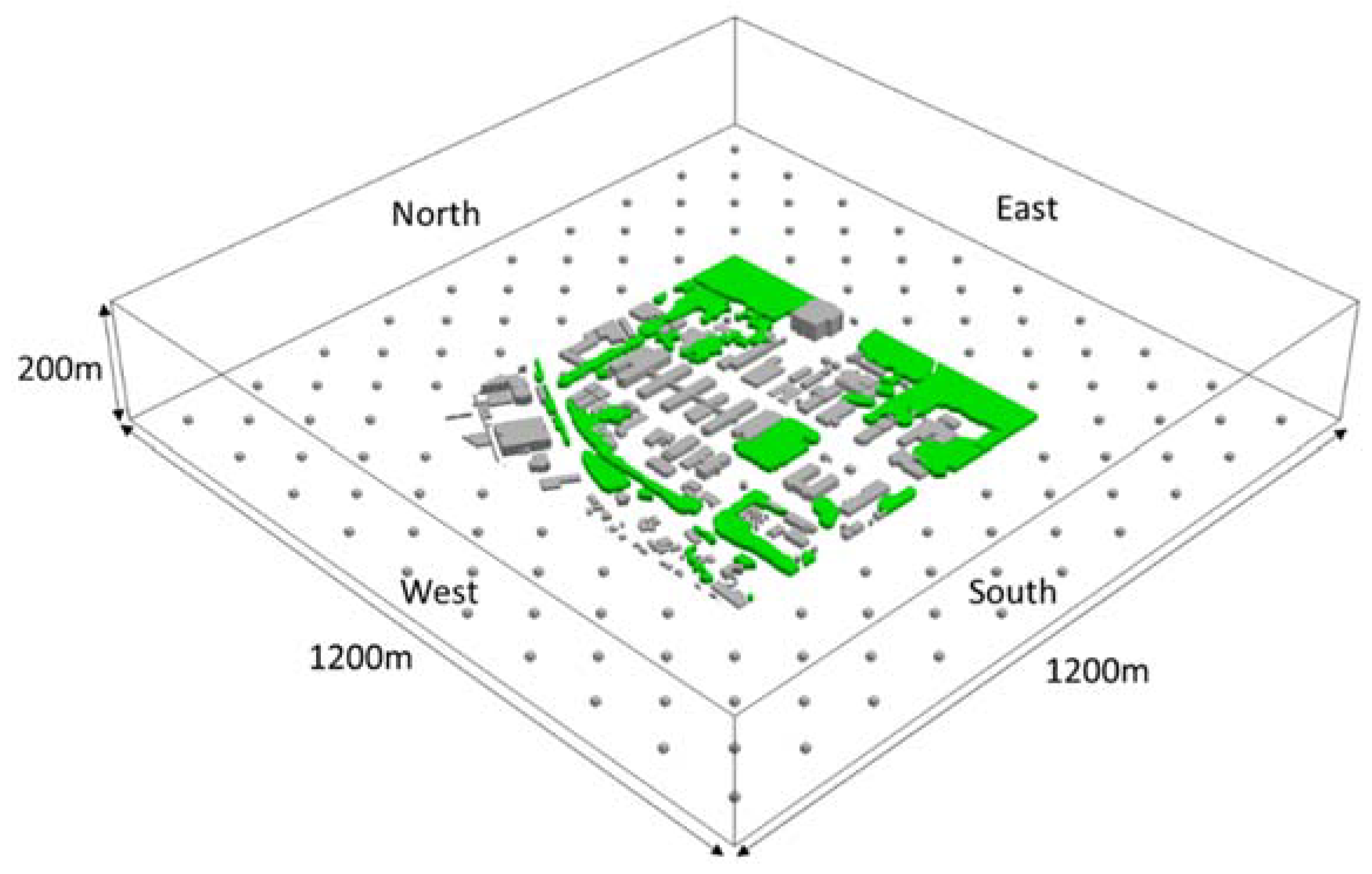
3.2. Computaiotnal Conditions

Figure 4 shows the computational domain for creating the LES-database of mean and turbulent winds over the site of JAEA. The size of the computational domain is 1.2 km × 1.2 km in the horizontal direction at a depth of 200 m. The total mesh number is 1200 × 1200 × 88 nodes. The grid spacing is 1 m in the horizontal direction and 1–10 m stretched in the vertical direction. The buildings and tree canopy were explicitly resolved using a digital surface model dataset in the domain of 600 m × 600 m. The driver sections with a length of 300 m were set, and roughness blocks were placed to efficiently generate turbulent boundary layer (TBL) flows.

We pre-calculated LESs of TBL flows under a neutral stability condition and created a dataset of mean and turbulence velocities for 36 different mean wind directions at class interval 10°. The 10° class interval is enough to reasonably estimate spatial distributions of plume concentrations using the database for changing meteorological conditions [21]. A vertical profile with a power law exponent of 0.14 with a mean wind speed of 15 m/s at 60-m height was imposed at the inflow boundaries. At the same time, time-dependent turbulent inflow data were added to it by the recycling method [22]. At the bottom surface, the Monin-Obukhov similarity theory is applied [23]. The total length of the calculation run is 30 min. The first 20 min are considered to be the spin-up period before turbulent statistics become a statistical steady-state. The mean wind velocities and turbulence standard deviation were computed over the last 10-min period. The calculation time step interval is 0.005 s.

4. Dispersion Simulation Settings

4.1. Coupling of the LES-Database and On-Site OBS

The relationship between the lower atmospheric boundary layer and building morphological characteristics has been studied by many researchers. It is well known that boundary layer flows over buildings are mainly classified into three types: the building canopy layer, the roughness sublayer, and the inertial sublayer [24,25,26] as shown in Figure 5. In the building canopy layer, the flow patterns are directly determined by building arrangements and show a strong three-dimensionality caused by impinging, separated, and recirculating flows. The depth of the roughness sublayer ranges up to 2 to 5 times the height of the buildings [25]. In the inertial sublayer, the dynamical influence of the surface decreases with height and the flows eventually readjust to the meteorological conditions.

Figure 6 shows spatial distributions of the building heights represented by a digital surface model dataset. The averaging building height is 11.1 m. The building height variability defined as the ratio of the standard deviation of building height to the average building height is 5.1 m. The building height at this site is nearly uniform except the structure located at the east side. It is considered from this building morphological characteristics that the height at which the influence of buildings on atmospheric winds becomes fully small is approximately 55 m. Therefore, we took the measuring 6-points averaged winds obtained at 61.2-m height (elevation angle of 21.8°) for a reference meteorological condition.

Doppler LiDAR instruments can capture spatial distributions of wind velocities in real meteorological conditions. However, it was pointed out that those might include errors in representing high-frequency turbulent fluctuations [27]. Furthermore, buildings and trees cause obstructions of the laser beam at low elevation angles in certain azimuths [28]. On the other hand, LES models are intrinsically superior in capturing basic flow patterns within building canopy that are governed mainly by the building morphology under ideal meteorological conditions.

In this meteorological observation by the Doppler LiDAR, the radial wind velocities just above the building heights were measured for a case of elevation angle 1.0°. Therefore, first, in estimating a mean flow filed, we prepared the OBS data obtained by the Doppler LiDAR for the region above the building canopy layer and used the LES-database of mean velocities for the region below it.

$$U_{coup}\left(x,y,z\right)=U_{OBS}\left(x,y,h_{OBS}\left(x,y\right)\right)\mathrm{for}z>h_{OBS}\left(x,y\right)$$

(1)

$$U_{coup}\left(x,y,z\right)=U_{LES}\left(x,y,z\right)\frac{U_{OBS}\left(x,y,h_{OBS}\left(x,y\right)\right)}{U_{LES}\left(x,y,h_{OBS}\left(x,y\right)\right)}\mathrm{for}z\le h_{OBS}\left(x,y\right)$$

(2)

where $U_{coup}$, $U_{OBS}$, $U_{LES}$, and $h_{OBS}$ are the mean wind velocity estimated by a coupling of the LES-database and on-site OBS, the OBS wind velocity linearly interpolated on the LES calculation grids, the LES database of mean wind velocity, and the lowest measurement height of the Doppler LiDAR at the position of $\left(x,y\right)$, respectively. $U_{LES}$ is extracted from the LES-database pre-calculated for 36 different mean wind directions at class interval 10° in accordance with the target meteorological condition.

It is well known that the ratio of turbulence standard deviation to mean velocity is not constant and changes with the mean wind velocity for a weak wind condition, while the ratio is almost constant for a strong wind condition regardless of the mean velocity. The LES-database of mean and turbulence velocities was created under a strong neutral wind condition as mentioned in Section 3.2. The turbulence standard deviation can be estimated by multiplying the ratio in the LES-database by the mean wind velocity $U_{coup}$ for a strong wind condition. However, for a weak wind condition, the turbulence standard deviation can be no longer estimated by the product of them. Therefore, in estimating a turbulent flow field, we adopted Normal Turbulence Model (NTM) proposed by the International Electrotechnical Commission (IEC) in the international standard IEC61400-1 used for determining appropriate locations of wind turbines as shown in the following formulation [29].

$${\sigma }_l=I_{ref}\left(aU+b\right)$$

(3)

where ${\sigma }_l$ is the longitudinal turbulence standard deviation and $U$ is the mean wind speed at hub height over a 10-min period. $I_{ref}$ is the expected value of the turbulence intensity at 15 m/s and has three values of 0.12, 0.14, and 0.16 depending on wind turbine classes, respectively. The constants of $a$ and $b$ are 0.75 and 3.8, respectively, for the mean turbulence standard deviation. The measurements were taken at a height of the hub height of typically from 60 m to 80 m. The applicability of NTM IEC was investigated by Ishihara et al. [30].

To investigate the applicability to complex turbulent flow fields such as impinging, separated, and recirculating flows formed at building rooftop, regression analysis for $I_{ref}$ was conducted using the wind velocity data measured by the ultrasonic anemometer. When $I_{ref}$ = 0.16, the coefficient of determination shows a peak and its value is over 0.6 as shown in Figure 7a. It is also found from Figure 7b that the measurement data are generally distributed well along the NTM curve with $I_{ref}$ of 0.16, which indicates that the formulation is applicable to complex turbulent flow fields. Therefore, we applied it to strong three-dimensional turbulent flow fields within and over individual buildings as the following expression.

$${\sigma }_{l\_est}\left(x,y,z\right)=I_{ref\_l\_LES}\left(x,y,z\right)\left(a{U}_{coup}\left(x,y,z\right)+b\right)$$

(4)

$$I_{ref\_l\_LES}\left(x,y,z\right)=\frac{{\sigma }_{l\_LES}\left(x,y,z\right)}{U_{LES}\left(x,y,z\right)}$$

(5)

where ${\sigma }_{l\_est}$ is the estimated longitudinal turbulence standard deviation and $I_{ref\_l\_LES}$ is the longitudinal component of the local turbulence intensity given from the LES-database. Because it is difficult to derive two components of the turbulent fluctuations ${\sigma }_u$ and ${\sigma }_v$ directly from the longitudinal turbulence standard deviation ${\sigma }_l$, we assumed that ${\sigma }_l$ is equal to ${\sigma }_u$ for the measuring 6-points averaged wind direction $\theta$ ranging from 45° to 135° and from 225° to 315°, and ${\sigma }_l$ is equal to ${\sigma }_v$ for $\theta$ ranging from 0° to 45°, from 135° to 225°, and from 315° to 360°, respectively. When assuming ${\sigma }_l={\sigma }_u$ here, ${\sigma }_u$ can be estimated by the following formula.

$${\sigma }_{u\_est}\left(x,y,z\right)=I_{ref\_LES}\left(x,y,z\right)\left(a{U}_{coup}\left(x,y,z\right)+b\right)$$

(6)

$$I_{ref\_LES}\left(x,y,z\right)=\frac{{\sigma }_{u\_LES}\left(x,y,z\right)}{U_{LES}\left(x,y,z\right)}$$

(7)

The $v$- and $w$-components of the turbulence standard deviation were estimated by the following expression.

$${\sigma }_{v\_est}\left(x,y,z\right)=\frac{{\sigma }_{v\_LES}\left(x,y,z\right)}{{\sigma }_{u\_LES}\left(x,y,z\right)}{\sigma }_{u\_est}\left(x,y,z\right)$$

(8)

$${\sigma }_{w\_est}\left(x,y,z\right)=\frac{{\sigma }_{w\_LES}\left(x,y,z\right)}{{\sigma }_{u\_LES}\left(x,y,z\right)}{\sigma }_{u\_est}\left(x,y,z\right)$$

(9)

4.2. Lagrangian Particle Dispersion Model and Calculation Conditions

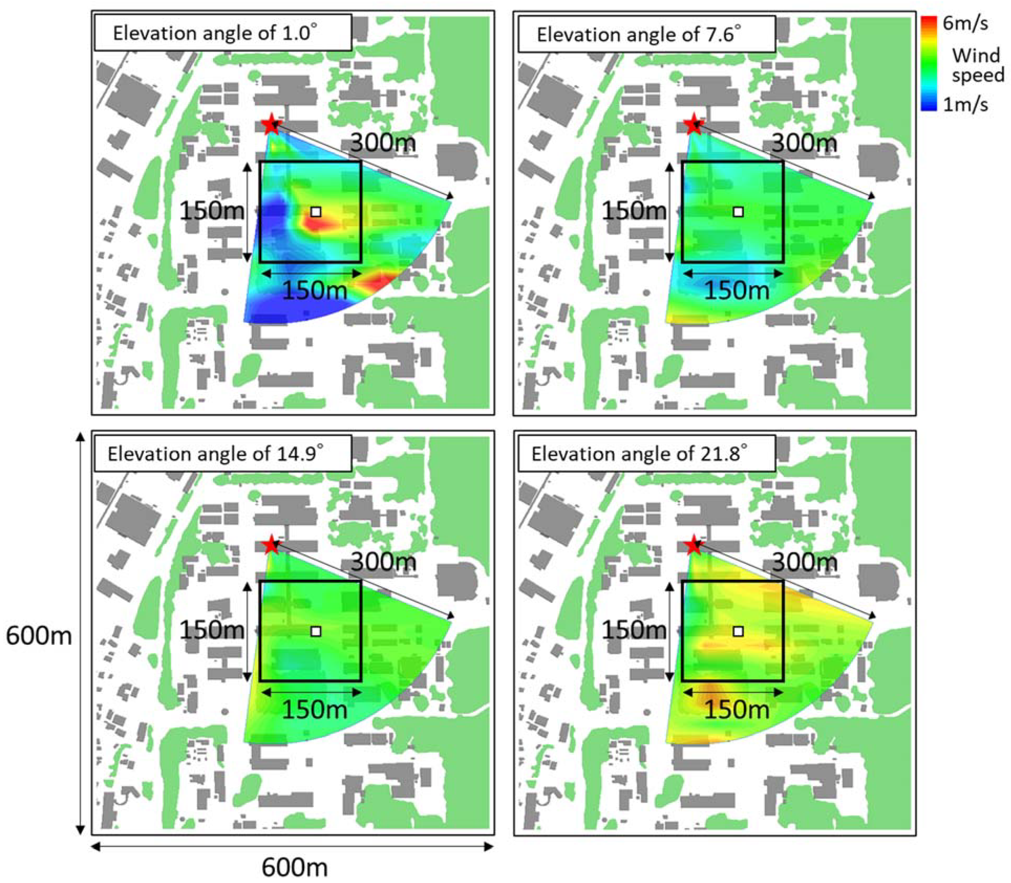
We adopted the following expression of a Lagrangian particle dispersion model [31].

$$x_i\left(t+\mathsf{\Delta }t\right)=x_i\left(t\right)+u_{pi}\mathsf{\Delta }t$$

(10)

$$u_{pi}=U_i+u_i^{\prime }$$

(11)

$$u_i^{\prime }\left(t+\mathsf{\Delta }t\right)=a{u}_i^{\prime }\left(t\right)+b{\sigma }_{ui}\xi +{\delta }_{i3}\left(1-a\right)t_{Lxi}\frac{\partial {\sigma }_{ui}^2}{\partial x_i}$$

(12)

$$a=exp\left(-\frac{\mathsf{\Delta }t}{t_{Lxi}}\right)$$

(13)

$$b={\left(1-a^2\right)}^{1/2}$$

(14)

where $x_i$, $u_{pi}$, $U_i$, $u_i^{\prime }$, ${\sigma }_{ui}$, $\xi$, $t_{Lxi}$, ${\delta }_i$, $t$, and $\mathsf{\Delta }t$ are the particle position in the i-direction (east-west direction, i = 1; north-south direction, i = 2; vertical direction, i = 3), velocity of the particle, mean wind velocity, turbulence velocity, standard deviation of the velocity fluctuation, a random number from a Gaussian distribution with zero mean and unit variance, the Lagrangian integral time, the Dirac delta function, time, and calculation time step interval, respectively.

The size of the computational domain is 150 m × 150 m in the horizontal direction at 100-m height as shown in Figure 2. The grid spacing and mesh arrangement are the same as the LES computational conditions as mentioned earlier. The target simulation periods are 10 min from 1122 JST to 1132 JST on 26 November 2020 and from 1112 JST to 1122 JST on 1 December 2020. The plume is released at 1.5-m height from the building rooftop. As described in the previous section, $U_i$ are provided from Equations (1) and (2). Each component of ${\sigma }_i$ was given by Equations (6), (8) and (9). The particles are assumed to be reflected at the solid boundaries. The calculation time step interval is 0.05 s. The number of the imaginary particles is 3600.

5. Results

Figure 8 shows horizontal distributions of the Doppler LiDAR-derived wind velocity vectors near the mist plume release height for the two experimental periods of the case A from 1125 to 1131 JST 26 November and the case B from 1116 to 1122 JST 1 December. The wind velocities were interpolated on the grids of 1 m × 1 m. For the case A, first, a western wind blew around the release location and a northwesterly wind was also overserved on the north side from there. Then, a north-northwest wind blew just in the west side and a west wind did in the east side from the release point. At 1131 JST, a west-northwest and northwest wind blew in the whole area. For the case B, first, a northeast wind blew just in the northeast area, southeaste wind did in the southeast area, and an east wind blew in the vicinity of the release point. A vortex weak wind rotating counterclockwise was also observed in the southwest side. Then, an east wind blew in the whole area. The main flow directions above the building canopy changed from 280° to 304° and from 75° to 118° during the periods for the cases A and B, respectively. It is found that the wind direction variability is larger for the case B.

Figure 9 shows instantaneous dispersion shots of the mist plume generated by the mist-spraying system at 3-min interval over the 10-min period after the release for the two cases. Here, the 10-min period was selected as the sampling period for investigating general behaviors of the plume under the influence of turbulent-scale flows. Macdonald and Griffiths [32] and Macdonald et al. [33] investigated plume dispersion behavior over regular arrays of building-like obstacles at a field site. In their field experiments, the 3-min period was selected as the standard sampling period for mean concentration because the time period less than 15–20-min removes the influence of the lateral meandering of a plume due to the meteorological disturbances. For the case A, it is observed that the mist plume was constantly transported in the east from the plume release location. On the other hand, for the case B, the mist plume centroid was actively fluctuated around the general transport direction in the west. This is due to the separated turbulent flows formed at the corner of the building. The horizontal transport direction of the plume generally corresponds to the Doppler LiDAR-derived wind velocity vectors for both cases.

Figure 10 shows 3-dimensional distributions of 10-min averaged concentrations of the simulated plume for the cases A and B. Concentration at each mesh was estimated by kernel density estimation [31]. For the case A, the plume is transported in the east and a part of the plume is entrained into the zone of recirculating flow behind the building. For the case B, the plume is transported in the west and a part of the plume is entrained into the gap between the buildings due to the channeling effects. When compared both cases, it is also found that the plume spreads for the case B are larger than the ones for the case A. This is because the initial plume spreads are enhanced by the strong turbulence intensities produced at the building corner.

These results indicate that the general transport direction of the simulated plume is reproduced well by using the Doppler LiDAR-derived wind velocities for the region above the building canopy layer in comparison with the instantaneous shots of the real mist plume shown in Figure 9. The entrainment behavior of the plume into the building wake is also qualitatively represented well by using the LES-database for the region below it. Furthermore, the relative size of the simulated plume between the two cases can be associated with the fact that the fluctuating patterns of the real mist plume centroid, which implies that the local turbulence velocities are reasonably estimated from the empirical formulation of the relationship between mean wind speed and turbulence standard deviation. Therefore, it is concluded that our proposed framework for prediction system of local-scale atmospheric dispersion based on a coupling of LES-database and on-site meteorological observation has an enough potential to simulate plume transport direction by mean winds and reasonably represent dispersion behaviors by turbulence under the influences of individual buildings and meteorological disturbances.

6. Conclusions

We developed a framework for prediction system of local-scale atmospheric dispersion based on a coupling of LES-database and on-site meteorological observation that takes into account both individual buildings and real meteorological conditions. First, we performed LESs of turbulent flows over a target site and created the dataset of mean and turbulent flows for 36 mean wind directions at 10° class interval. Then, we conducted with meteorological observations by a Doppler LiDAR and simple dispersion experiments using a mist-spraying system at the target site, and observed dispersion behaviors of the water mist plume using a digital camera.

In estimating a mean flow filed, we prepared the OBS data obtained by the Doppler LiDAR for the region above the building canopy layer and used the LES-database of mean velocities for the region below it. In estimating a turbulent flow field, we adopted the empirical formulation of the relationship between mean wind speed and turbulence standard deviation used for determining appropriate locations of wind turbines. Compared to instantaneous shots of dispersion behaviors of the real mist plume, it was shown that the transport direction of the simulated plume was reproduced well by the Doppler LiDAR-derived wind velocities. The entrainment behavior of the plume into the building wake was qualitatively represented well by the LES-database. Furthermore, the plume spreads were also reasonably represented well by the estimated local turbulence velocities from the empirical formulation.

Here, we discuss the feasibility of our proposed framework for prediction system of local-scale atmospheric dispersion a as a practical emergency response system. Since computing time is an essential problem for emergency situations, first result should be provided within a few minutes especially in local-scale emergency response [34]. Our dispersion calculations by this coupling of the LES-database and on-site OBS were executed on a single core of an Intel CPU. The calculation time was approximately 15 s in order to simulate plume concentrations in the target computational domain of 150 m × 150 m × 50 m at 1 m grid. In conducting CFD simulations of turbulent flows and/or plume dispersion in a local-scale, the target site usually has a computational domain size of several kilometers at grid spacing of several meters for the horizontal direction. Considering it, the estimated calculation time is a few minutes. These facts indicate that our proposed coupling of the LES-database and on-site OBS is effective to accurately and quickly predict plume dispersion under the influences of both individual buildings and real meteorological conditions.

For the areas that are not covered by the measurements or for a case that the wind LiDAR is not available, a meso-scale meteorological simulation (MMS) model data should be used. Recently, coupling simulations of CFD and MMS models have been studied and evaluated against the urban tracer field experiments by many researchers [35,36,37]. We also conducted LESs of plume dispersion in the real urban central district by coupling with the MMS model and showed the reasonable performance of simulating plume dispersion in the built-up area under realistic meteorological conditions [17].

In future work, it is necessary to conduct field dispersion experiments on tracer gas release in a local-scale distances of up to several kilometers. We previously conducted LESs of plume dispersion in various urban areas with a wide range of obstacle density and building height variability, and compared the streamwise variation of mean and r.m.s. concentrations. It was shown that the spatial extent of concentration distribution patterns influenced by complex surface geometry is 1 km from a point source by comparative analysis [38]. Furthermore, it was reported that the assumption of a neutral stability is valid for within an urban area where building-induced turbulence is dominant and the assumption is less valid for the urban wake region because the levels of building-induced turbulence greatly subside [39]. It is necessary to quantitatively evaluate the coupling framework in comparison with the field experimental data at many downstream positions under thermal stability conditions in a local-scale distances of up to several kilometers. When fully evaluating it, our proposed technique is expected to use in source term estimation for contaminant plume dispersion in emergency responses to accidental release from nuclear facilities.

References

1. Murakami, S.; Mochida, A.; Hayashi, Y. Examining the κ-ε model by means of a wind tunnel test and large-eddy simulation of the turbulence structure around a cube. J. Wind Eng. Ind. Aerodyn. 1990, 35, 87–100. [Google Scholar] [CrossRef]
2. Tominaga, Y.; Stathopoulos, T. Numerical simulation of dispersion around an isolated cubic building, Model evaluation of RANS and LES. Build. Environ. 2010, 45, 2231–2239. [Google Scholar] [CrossRef] [Green Version]
3. Tominaga, Y.; Stathopoulos, T. CFD modeling of pollution dispersion in a street canyon: Comparison between LES and RANS. J. Wind Eng. Ind. Aerodyn. 2011, 99, 340–348. [Google Scholar] [CrossRef] [Green Version]
4. Gousseau, P.; Blocken, B.; Stathopoulos, T.; Heijst, G. CFD simulation of near-field pollutant dispersion on a high-resolution grid: A case study by LES and RANS for a building group in downtown Montreal. Atmos. Environ. 2011, 45, 428–438. [Google Scholar] [CrossRef] [Green Version]
5. Santiago, J.; Martilli, A. A dynamic urban canopy parameterization for mesoscale models based on computational fluid dynamics Reynolds–averaged Navier–Stokes microscale simulations. Bound. Layer Meteorol. 2010, 137, 417–439. [Google Scholar] [CrossRef]
6. Tominaga, Y.; Stathopoulos, T. CFD modeling of pollution dispersion in building array: Evaluation of turbulent scalar flux modeling in RANS model using LES results. J. Wind Eng. Ind. Aerodyn. 2012, 104, 484–491. [Google Scholar] [CrossRef] [Green Version]
7. Tominaga, Y.; Stathopoulos, T. CFD simulation of near-field pollutant dispersion in the urban environment: A review of current modeling techniques. Atmos. Environ. 2013, 79, 716–730. [Google Scholar] [CrossRef] [Green Version]
8. Yoshida, T.; Nakayama, H. Development of a combined LES/RANS model to predict atmospheric dispersion over urban areas. Jpn. Soc. Comput. Eng. Sci. 2020, 20200013. [Google Scholar]
9. Collier, C.G.; Davies, F.; Bozier, K.E.; Holt, A.R.; Middleton, D.R.; Pearson, G.N.; Siemen, S.; Willetts, D.V.; Upton, G.J.G.; Young, R.I. Dual-Doppler lidar measurements for improving dispersion models. Bull. Am. Meteorol. Soc. 2005, 86, 825–838. [Google Scholar] [CrossRef]
10. Yan, B.; Li, Q. Coupled on-site measurement/CFD based approach for high-resolution wind resource assessment over complex terrains. Energy Convers. Manag. 2016, 117, 351–366. [Google Scholar] [CrossRef]
11. Tang, X.Y.; Zhao, S.; Fan, B.; Peinke, J.; Stoevesandt, B. Micro-scale wind resource assessment in complex terrain based on CFD coupled measurement from multiple masts. Appl. Energy 2019, 238, 806–815. [Google Scholar] [CrossRef]
12. Radunz, W.C.; Mattuella, J.M.; Petry, A.P. Wind resource mapping and energy estimation in complex terrain: A framework based on field observations and computational fluid dynamics. Renew. Energy 2020, 152, 494–515. [Google Scholar] [CrossRef]
13. Nakano, M.; Watanabe, H.; Sumiya, S. Examination on the Long-Term Practicability of a Doppler Lidar-Data Missing Rate and Comparison of Wind Direction and Speed with the Propeller Type; Japan Atomic Energy Agency: Tokyo, Japan, 2013. (In Japanese) [Google Scholar]
14. Hashimoto, K.; Hori, A.; Hara, T.; Onogi, S.; Mouri, H. Dual-camera system for high-speed imaging of particle image velocimetry. J. Vis. 2012, 15, 193–195. [Google Scholar] [CrossRef] [Green Version]
15. Onogi, S.; Haginoya, S.; Hori, A.; Yagi, T.; Mouri, H. Field PIV imaging technique with consumer digital still cameras. J. Wind. Eng. 2014, 39, 63–66. (In Japanese) [Google Scholar] [CrossRef] [Green Version]
16. Nakayama, H.; Leitl, B.; Harms, F.; Nagai, H. Development of local-scale high-resolution atmospheric dispersion model using large-eddy simulation part 4: Turbulent flows and plume dispersion in an actual urban area. J. Nucl. Sci. Technol. 2014, 51, 626–638. [Google Scholar] [CrossRef] [Green Version]
17. Nakayama, H.; Takemi, T.; Nagai, H. Development of local-scale high-resolution atmospheric dispersion model using large-eddy simulation part 5: Detailed simulation of turbulent flows and plume dispersion in an actual urban area under real meteorological conditions. J. Nucl. Sci. Technol. 2016, 53, 887–908. [Google Scholar] [CrossRef]
18. Nakayama, H.; Satoh, D.; Nagai, H.; Terada, H. Development of local-scale high-resolution atmospheric dispersion model using large-eddy simulation part 6: Introduction of detailed dose calculation method. J. Nucl. Sci. Technol. 2021, 1–21. [Google Scholar] [CrossRef]
19. Smagorinsky, J. General circulation experiments with the primitive equations. Mon. Weather Rev. 1963, 91, 99–164. [Google Scholar] [CrossRef]
20. Goldstein, D.; Handler, R.; Sirovich, L. Modeling a no-slip flow boundary with an external force field. J. Comput. Phys. 1993, 105, 354–366. [Google Scholar] [CrossRef] [Green Version]
21. Nakayama, H.; Takemi, T. Large-eddy simulation studies for predicting plume concentrations around nuclear facilities using an overlapping technique. Int. J. Environ. Pollut. 2018, 64, 125–144. [Google Scholar] [CrossRef]
22. Kataoka, H.; Mizuno, M. Numerical flow computation around aeroelastic 3D square cylinder using inflow turbulence. Wind Struct. 2002, 5, 379–392. [Google Scholar] [CrossRef]
23. Monin, A.; Obukhov, M. Basic laws of turbulent mixing in the ground layer of the atmosphere. Tr. Akad. Nauk SSSR Geophiz. Inst. 1954, 24, 163–187. [Google Scholar]
24. Grimmond, C.S.B.; Oke, T.R. Turbulent heat fluxes in urban areas: Observations and a local-scale urban meteorological parameterization scheme (LUMPS). J. Appl. Meteorol. 2002, 41, 792–810. [Google Scholar] [CrossRef] [Green Version]
25. Cheng, H.; Castro, I.P. Near wall flow over urban-like roughness. Bound. Layer Meteorol. 2002, 104, 229–259. [Google Scholar] [CrossRef]
26. Britter, R.E.; Hanna, S.R. Flow and dispersion in urban areas. Annu. Rev. Fluid Mech. 2003, 35, 469–496. [Google Scholar] [CrossRef]
27. Yoshida, T.; Takemi, T.; Horiguchi, M. Large-eddy-simulation study of the effects of building-height variability on turbulent flows over an actual urban area. Bound. Layer Meteorol. 2018, 168, 127–153. [Google Scholar] [CrossRef] [Green Version]
28. Newson, R.K.; Calhoun, R.; Heap, R.; Cregan, E.; Princevac, M. Retrieval of microscale wind and temperature fields from single- and dual-Doppler lidar data. J. Appl. Meteorol. 2005, 44, 1324–1345. [Google Scholar] [CrossRef]
29. IEC61400-1. Wind Turbines Part 1: Design Requirements, 3rd ed.; International Electrotechnical Commission: Geneva, Switzerland, 2005. [Google Scholar]
30. Ishihara, T.; Yamaguchi, A.; Sarwar, M.W. A study of the Normal Turbulence Model in IEC 61400-1. Wind Eng. 2012, 36, 759–766. [Google Scholar] [CrossRef]
31. Yamada, T.; Bunker, S. Development of a nested grid, second moment turbulence closure model and application to the 1982 ASCOT Brush Creek data simulation. J. Appl. Meteorol. Climatol. 1988, 562–578. [Google Scholar] [CrossRef] [Green Version]
32. MacDonald, R.W.; Griffiths, R.F.; Cheah, S.C. Field experiments of dispersion through regular arrays of cubic structures. Atmos. Environ. 1997, 31, 783–795. [Google Scholar] [CrossRef]
33. Macdonald, R.W.; Griffiths, R.F.; Hall, D.J. A comparison of results from scaled field and wind tunnel modeling of dispersion in arrays of obstacles. Atmos. Environ. 1998, 32, 3845–3862. [Google Scholar] [CrossRef]
34. Leitl, B.; Harms, F.; Berbekar, E.; Boris, J.; Patnaik, G.; Obenschain, K.; Fischer, S. Local-scale hazmat dispersion modelling for first responders based on high-resolution computational fluid dynamics-an overview of CT-Analyst Hamburg. Chem. Eng. Trans. 2016, 48, 43–48. [Google Scholar]
35. Nelson, M.A.; Brown, M.J.; Halverson, S.A.; Bieringer, P.; Annunzio, A.; Bieberbach, G.; Meech, S. A case study of the weather research and forecasting model applied to the joint urban 2003 tracer field experiment. part 1: Wind and turbulence. Bound. Layer Meteorol. 2016, 158, 285–309. [Google Scholar] [CrossRef]
36. Nelson, M.A.; Brown, M.J.; Halverson, S.A.; Bieringer, P.; Annunzio, A.; Bieberbach, G.; Meech, S. A case study of the weather research and forecasting model applied to the joint urban 2003 tracer field experiment. Part 2: Gas Tracer Dispersion. Bound. Layer Meteorol. 2016, 161, 461–490. [Google Scholar] [CrossRef]
37. Burman, J.; Jonsson, L.; Rutgersson, A. On possibilities to estimate local concentration variations with CFD-LES in real urban environments. Environ. Fluid Mech. 2019, 19, 719–750. [Google Scholar] [CrossRef] [Green Version]
38. Nakayama, H.; Jurcakova, K.; Nagai, H. Large-Eddy Simulation of plume dispersion within various actual urban areas. Adv. Sci. Res. 2010, 10, 33–41. [Google Scholar] [CrossRef] [Green Version]
39. Lundquist, J.K.; Chan, S.T. Consequences of urban stability conditions for computational fluid dynamics simulations of urban dispersion. J. Appl. Meteorol. Climatol. 2007, 46, 1080–1097. [Google Scholar] [CrossRef] [Green Version]
Figure 1. Locations of the meteorological observations and the mist-spraying system. (a) Study site in JAEA. (b) Doppler LiDAR and sonic anemometer. (c) Mist-spraying system. The photograph (a) is reproduced by GoogleTM earth graphic. The red star depicts a position of the Doppler LiDAR and sonic anemometer placed at the building rooftop. The yellow circles are measurement points of wind velocity by the Doppler LiDAR at elevation angle of 1.0°. The white square depicts a position of the mist-spraying system placed at the building rooftop. The white arrow indicates a position of the digital camera on the ground directed toward the mist-spraying system.
Atmosphere 12 00899 g001
Figure 2. Spatial distributions of radial wind speeds at elevation angles of 1.0°, 7.6°, 14.9°, and 21.8° on 1122 JST 26 November 2020. The square indicates the computational domain used for calculating plume dispersion. The symbols are the same as in Figure 1. The gray and green areas indicate buildings and tree canopy, respectively. The gray and green areas are buildings and tree canopy, respectively.
Atmosphere 12 00899 g002
Figure 3. Photograph of the mist plume generated by the mist-spraying system.
Atmosphere 12 00899 g003
Figure 4. Computational domain for creating the LES-database of mean and turbulent winds over the target site.
Atmosphere 12 00899 g004
Figure 5. Schematic of TBL flows over buildings. Adopted from Britter and Hanna [27].
Atmosphere 12 00899 g005
Figure 6. Spatial distributions of building heights in the site of JAEA represented using the digital surface model dataset. The symbols of the red star and the white square are the same as in Figure 1. The yellow circles are measurement points of the Doppler LiDAR at elevation angle of 21.8° used for estimating the reference meteorological condition.
Atmosphere 12 00899 g006
Figure 7. The coefficient of determination for regression analysis (a) and variation of the turbulence intensity with the mean wind speed measured by the ultrasonic anemometer placed at the building rooftop (b).
Atmosphere 12 00899 g007
Figure 8. Horizontal distributions of the Doppler LiDAR-derived wind velocity vectors near the mist plume release height. The areas correspond to the square area of 150 m × 150 m shown in Figure 1. The white square depicts a position of the mist-spraying system placed at the building rooftop. The arrow indicates a position of the digital camera on the ground directed toward the mist-spraying system. The case A is the period from 1125 to 1131 JST 26 November. The case B is the period from 1116 to 1122 JST 1 December.
Atmosphere 12 00899 g008
Figure 9. Instantaneous shots of the mist plume dispersion generated by the mist-spraying system at 3-min interval (a) and the simulated plume dispersion (b). The dashed line indicates the enveloping contour of the mist plume. The photograph was taken by the digital camera directed toward the mist-spraying system as shown in Figure 1. The yellow areas indicate the 50% iso-surface of initial concentration.
Atmosphere 12 00899 g009
Figure 10. 10-min averaged concentrations of the simulated plume. The yellow areas indicate the 5% iso-surface of initial concentration. The blue circle is the release point.
Atmosphere 12 00899 g010
Publisher’s Note: MDPI stays neutral with regard to jurisdictional claims in published maps and institutional affiliations.