
Changes in Power Plant NOx Emissions over Northwest Greece Using a Data Assimilation Technique

 , , , , , and
Abstract
:1. Introduction
2. Materials and Methods
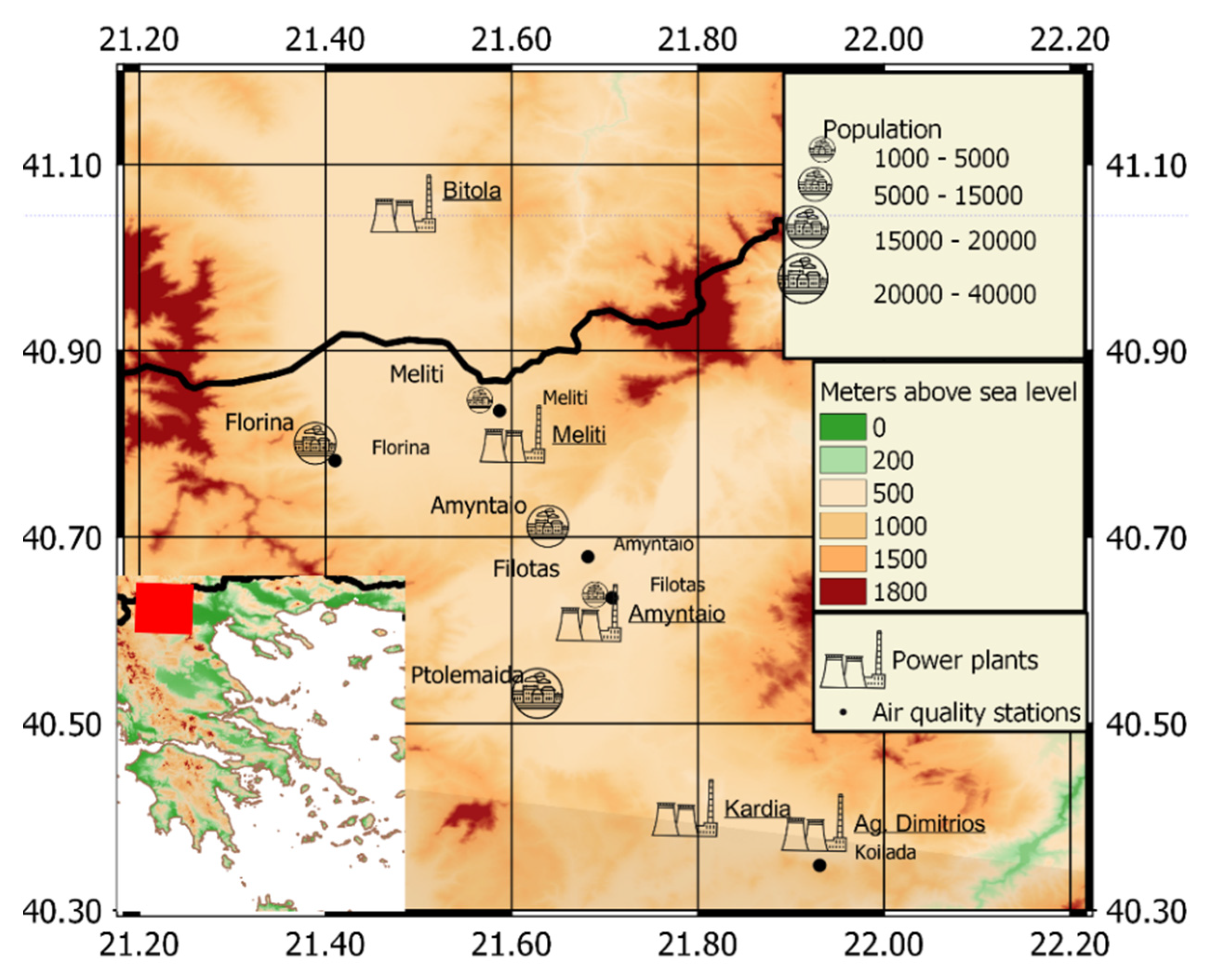
2.1. Power Plants in Northwest Greece
2.2. The LOTOS-EUROS CTM
2.3. The A Priori NOx Emissions
2.4. The S5P/TROPOMI Satellite Observations
2.5. Ensemble Kalman Filter around LOTOS-EUROS CTM
2.6. In Situ NO2 Measurements
3. Results and Discussion
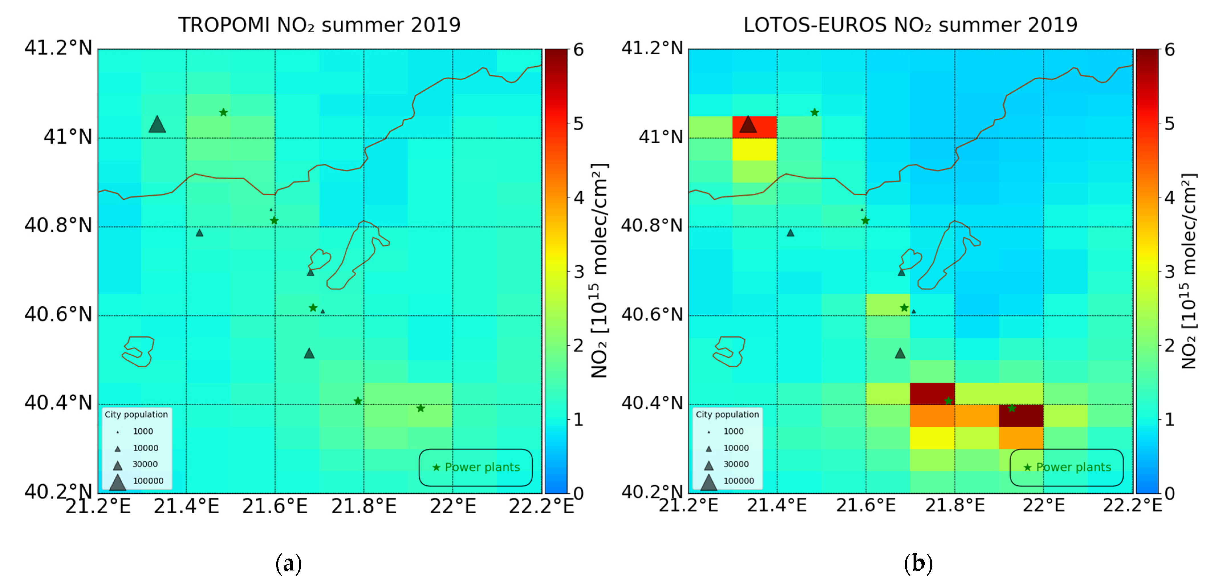
3.1. LOTOS-EUROS NO2 Simulations and S5P/TROPOMI Observations
3.2. Updated Assimilated NOx Emissions
3.3. Validation of the A Posteriori NOx Simulations
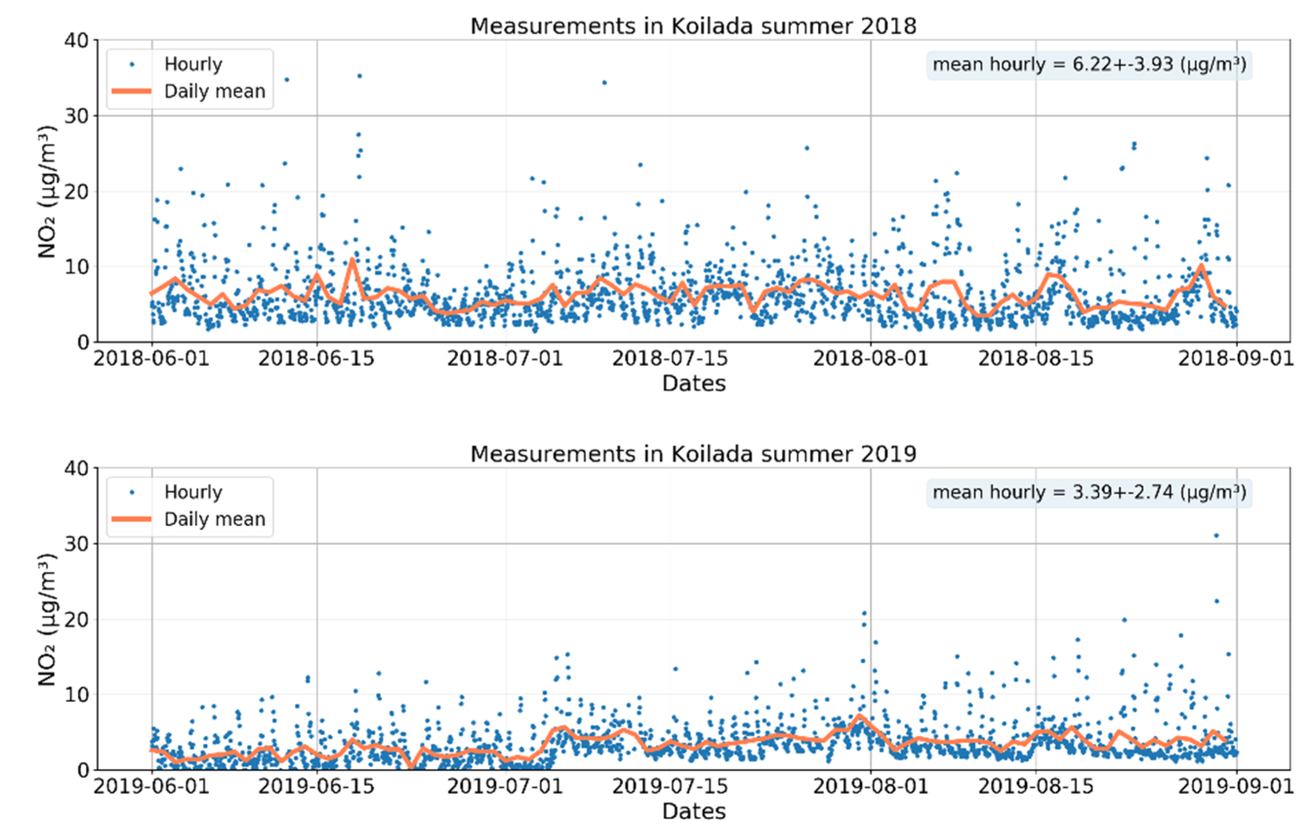
3.3.1. In Situ Measurements
3.3.2. Energy Production of the Power Plants
4. Conclusions
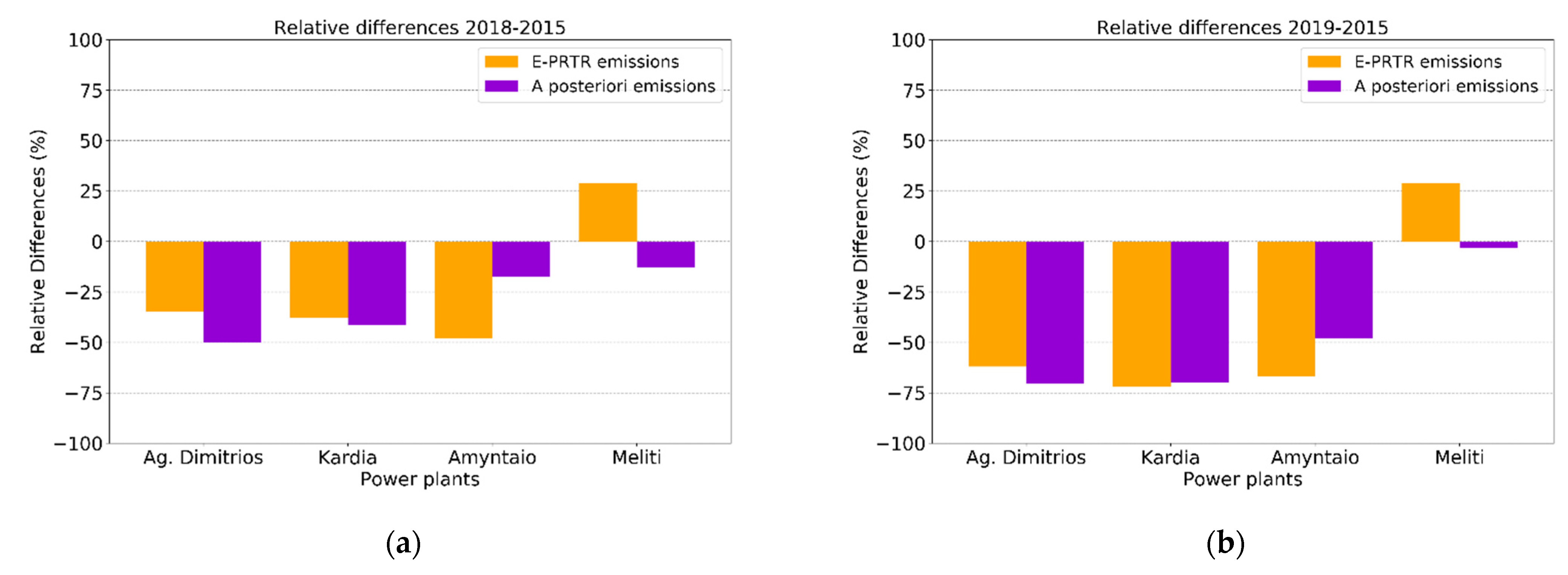
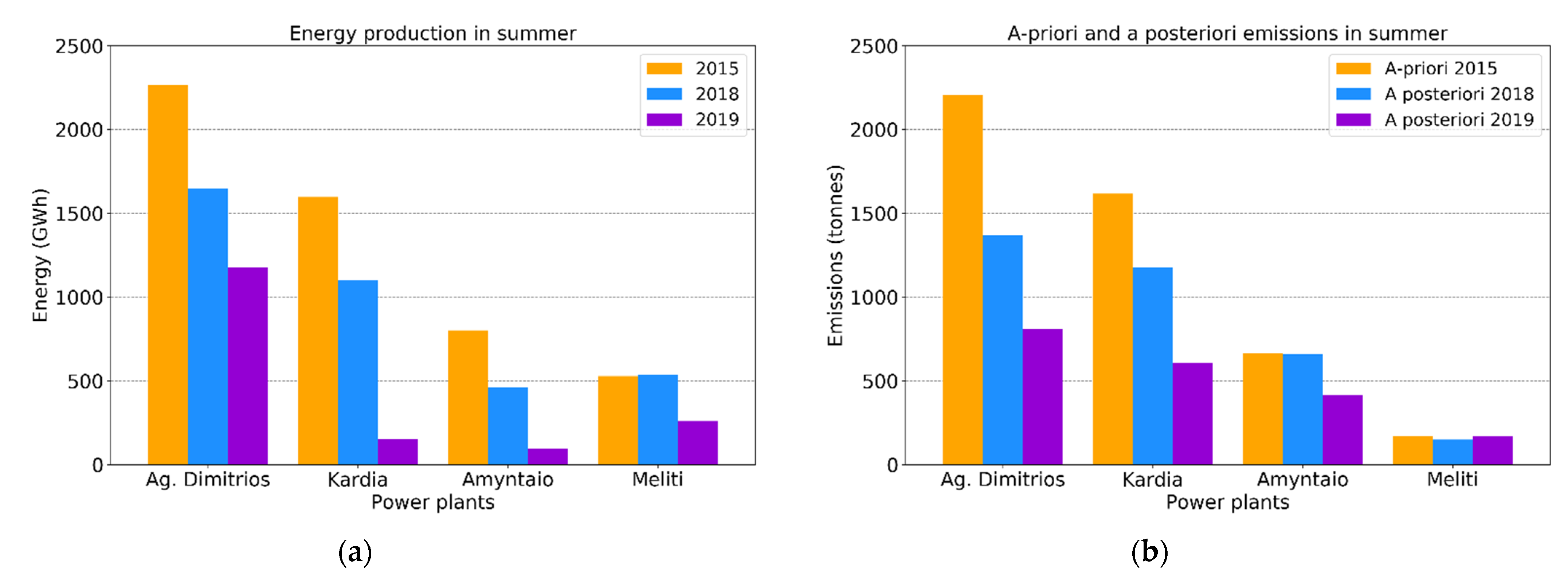
- For 2019, the summertime a posteriori emissions estimated for the two largest power plants of Ag. Dimitrios and Kardia decreased by more than 60% compared to the a priori 2015 emissions, while in 2018 they are reduced by around 33%.
- Stronger decreases in the energy production are reported for the summer period of 2019 compared to the summer of 2018 as well, in line with the estimated emission reduction. The energy production of the Ag. Dimitrios power plant decreased by around 50% in 2019 compared to 2015, while in Kardia and Amyntaio energy decreased by 90% for the summer of 2019. In the summer of 2018, the energy production in the three larger power plants decreased by around 30–45%.
- The a posteriori annual emission changes estimated over the two larger power plants in 2018 compared to the a priori 2015 emissions are ~−40% to −50%, whereas the changes for 2019 are ~−70% for both power plants. These a posteriori annual NOx emissions agree well in line with the annual emissions reported by E-PRTR. The changes in the annual E-PRTR 2018 reported emissions compared to 2015 over Ag. Dimitrios and Kardia are −35% and −38%, while for 2019 this decrease rises to −62% and −72%, closely following the findings of this work.
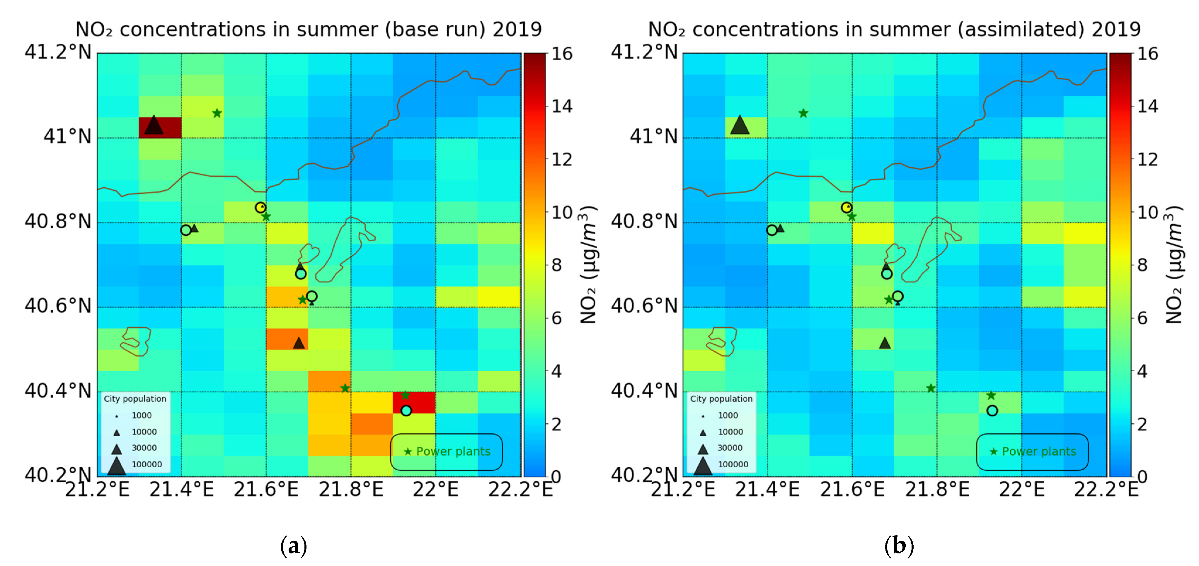
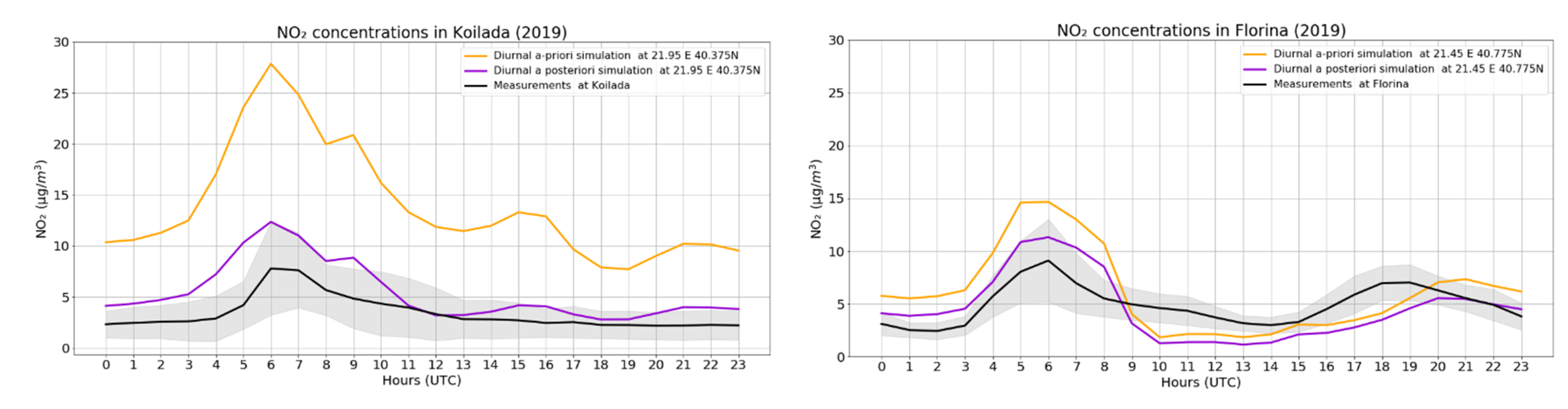
- In situ NO2 measurements from air quality stations of Koilada and Amyntaio, which are directly affected by pollution from the power plants of Ag. Dimitrios and Amyntaio, show an improved agreement with the assimilated NO2 simulations compared to the base run which is based on the 2015 CAMS a priori emissions. The bias in the station of Koilada near the power plant of Ag. Dimitrios improves to 2 μg/m3 (2.83 μg/m3) from 10.5 μg/m3 (8.46 μg/m3) in 2019 (2018).
- The results for the Meliti power plant were found not to be representative of the grid cell where the plant is located due to presence of other emission sources affecting that grid cell. The dominant winds over the neighboring Bitola power plant are northerly for both summers of 2018 and 2019, showing that pollution may flow from the neighboring country of Republic of North Macedonia towards Northwest Greece.
Supplementary Materials
Author Contributions
Funding
Institutional Review Board Statement
Informed Consent Statement
Data Availability Statement
Acknowledgments
Conflicts of Interest
Appendix A

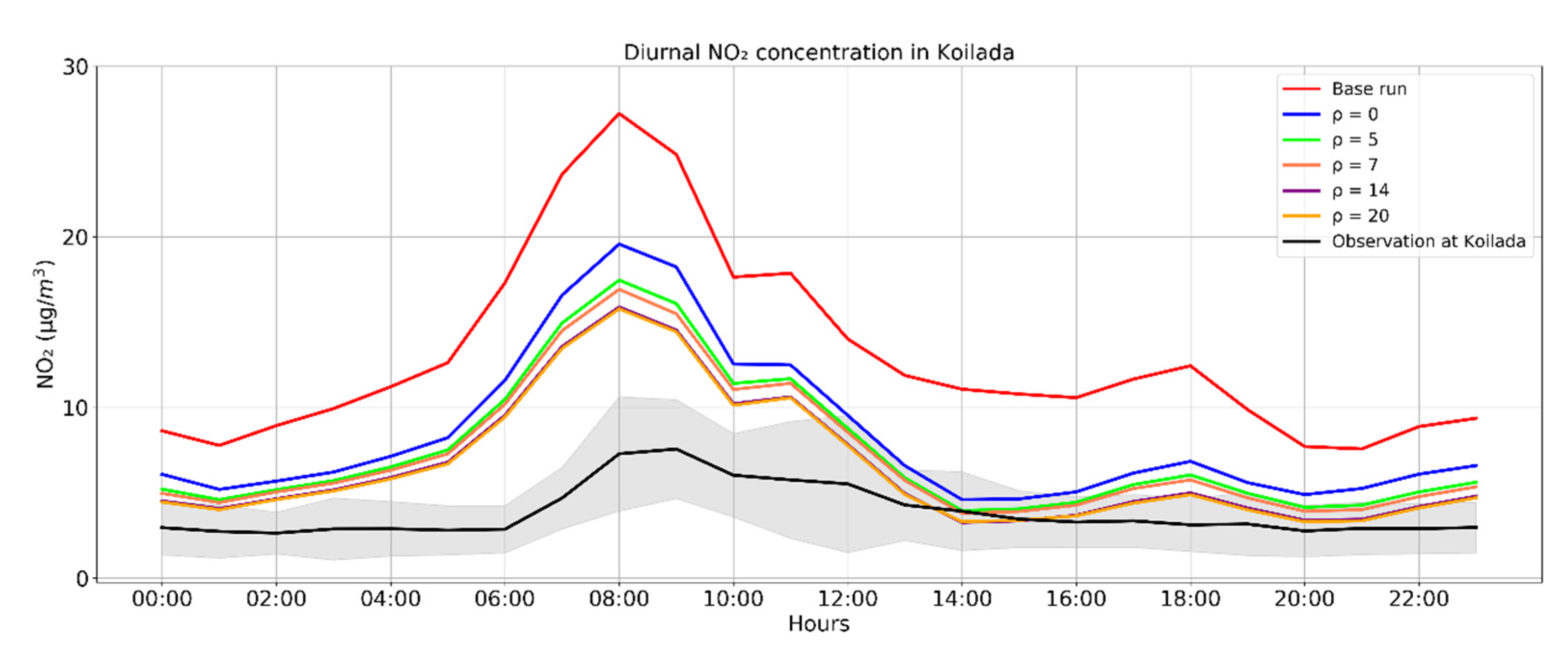
| Localization Radius (ρ) in km | |||
|---|---|---|---|
| Configuration | Mean | Bias | RMSE |
| Base run | 13.05 | 9.17 | 12.21 |
| ρ = 0 | 8.37 | 4.49 | 7.40 |
| ρ = 5 | 7.46 | 3.58 | 6.36 |
| ρ = 7 | 7.20 | 3.31 | 6.01 |
| ρ = 14 | 6.56 | 2.68 | 5.31 |
| ρ = 20 | 6.49 | 2.61 | 5.23 |
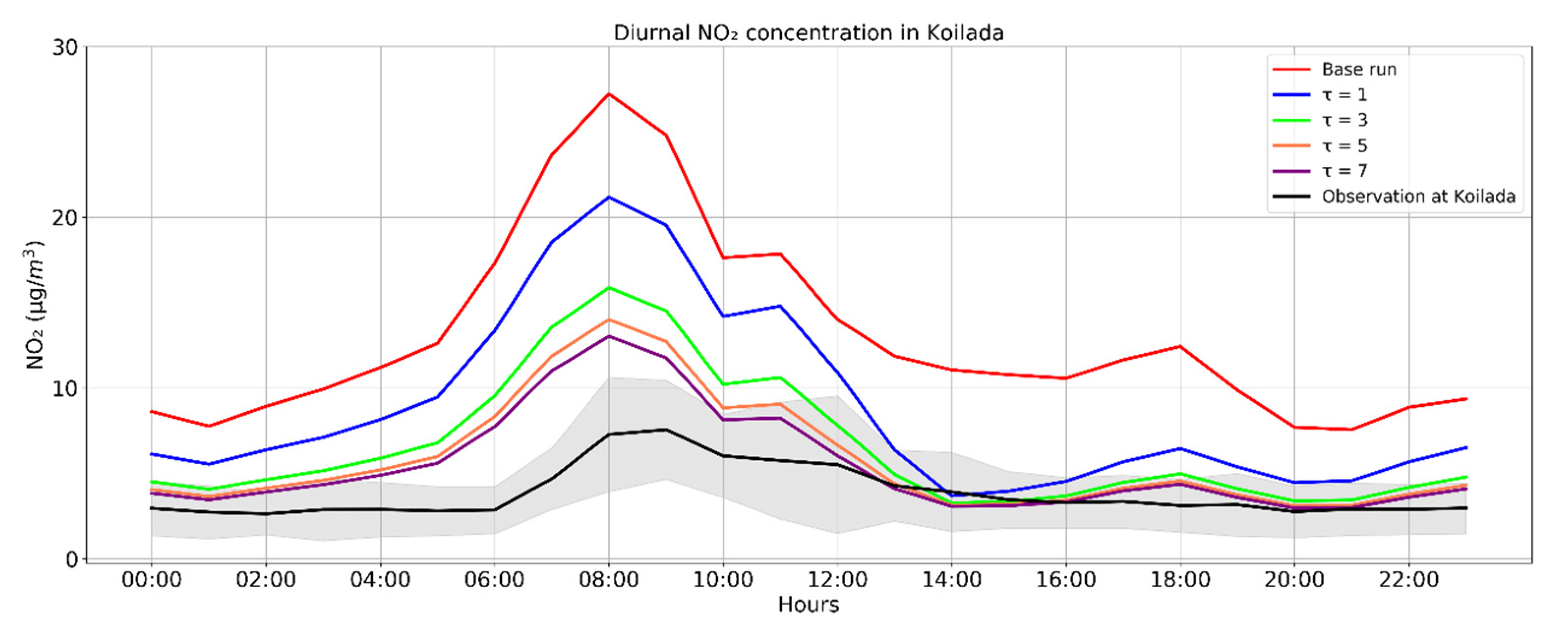
| Temporal correlation parameter (τ) in days | |||
| Configuration | Mean | Bias | RMSE |
| Base run | 13.05 | 9.17 | 12.21 |
| τ = 1 | 8.83 | 4.95 | 8.04 |
| τ = 3 | 6.56 | 2.68 | 5.31 |
| τ = 5 | 5.82 | 1.94 | 4.52 |
| τ = 7 | 5.46 | 1.57 | 4.18 |

References
- Varshney, C.K.; Singh, A.P. Passive samplers for NOx monitoring: A critical review. Environmentalist 2003, 23, 127–136. [Google Scholar] [CrossRef]
- Miyazaki, K.; Eskes, H.J.; Sudo, K. Global NOx emission estimates derived from an assimilation of OMI tropospheric NO2 columns. Atmos. Chem. Phys. 2012, 12, 2263–2288. [Google Scholar] [CrossRef] [Green Version]
- Streets, D.G.; Bond, T.C.; Carmichael, G.R.; Fernandes, S.D.; Fu, Q.; He, D.; Klimont, Z.; Nelson, S.M.; Tsai, N.Y.; Wang, M.Q.; et al. An inventory of gaseous and primary aerosol emissions in Asia in the year 2000. J. Geophys. Res. Atmos. 2003, 108. [Google Scholar] [CrossRef]
- Müller, J.-F.; Stavrakou, T. Inversion of CO and NO2 emissions using the adjoint of the IMAGES model. Atmos. Chem. Phys. 2005, 5, 1157–1186. [Google Scholar] [CrossRef] [Green Version]
- Castellanos, P.; Boersma, K.F. Reductions in nitrogen oxides over Europe driven by environmental policy and economic recession. Sci. Rep. 2012, 2, 1–7. [Google Scholar] [CrossRef]
- Duncan, B.N.; Lamsal, L.N.; Thompson, A.M.; Yoshida, Y.; Lu, Z.; Streets, D.G.; Hurwitz, M.M.; Pickering, K.E. A space-based, high-resolution view of notable changes in urban NOx pollution around the world (2005–2014). J. Geophys. Res. 2016, 121, 976–996. [Google Scholar] [CrossRef] [Green Version]
- Koukouli, M.E.; Skoulidou, I.; Karavias, A.; Parcharidis, I.; Balis, D.; Manders, A.; Segers, A.; Eskes, H.; Van Geffen, J. Sudden changes in nitrogen dioxide emissions over Greece due to lockdown after the outbreak of COVID-19. Atmos. Chem. Phys. 2021, 21, 1759–1774. [Google Scholar] [CrossRef]
- Bauwens, M.; Compernolle, S.; Stavrakou, T.; Müller, J.F.; van Gent, J.; Eskes, H.; Levelt, P.F.; Veefkind, J.P.; Vlietinck, J.; Yu, H.; et al. Impact of Coronavirus outbreak on NO2 pollution assessed using TROPOMI and OMI observations. Geophys. Res. Lett. 2020, 47, e2020GL087978. [Google Scholar] [CrossRef] [PubMed]
- Wu, H.; Tang, X.; Wang, Z.; Wu, L.; Li, J.; Wang, W.; Yang, W.; Zhu, J. High-spatiotemporal-resolution inverse estimation of CO and NOx emission reductions during emission control periods with a modified ensemble Kalman filter. Atmos. Environ. 2020, 236, 117631. [Google Scholar] [CrossRef]
- Evensen, G. Sequential data assimilation with a nonlinear quasi-geostrophic model using Monte Carlo methods to forecast error statistics. J. Geophys. Res. 1994, 99, 10143–10162. [Google Scholar] [CrossRef]
- Ding, J.; Van Der, A.R.J.; Mijling, B.; Levelt, P.F.; Hao, N. NOx emission estimates during the 2014 youth olympic games in Nanjing. Atmos. Chem. Phys. 2015, 15, 9399–9412. [Google Scholar] [CrossRef] [Green Version]
- Liu, F.; Beirle, S.; Zhang, Q.; Dörner, S.; He, K.; Wagner, T. NOx lifetimes and emissions of cities and power plants in polluted background estimated by satellite observations. Atmos. Chem. Phys. 2016, 16, 5283–5298. [Google Scholar] [CrossRef] [Green Version]
- Shah, V.; Jacob, D.J.; Li, K.; Silvern, R.; Zhai, S.; Liu, M.; Lin, J.; Zhang, Q. Effect of changing NOx lifetime on the seasonality and long-term trends of satellite-observed tropospheric NO2 columns over China. Atmos. Chem. Phys. 2020, 20, 1483–1495. [Google Scholar] [CrossRef] [Green Version]
- Triantafyllou, A.G. PM10 pollution episodes as a function of synoptic climatology in a mountainous industrial area. Environ. Pollut. 2001, 112, 491–500. [Google Scholar] [CrossRef]
- Levelt, P.F.; Joiner, J.; Tamminen, J.; Veefkind, J.P.; Bhartia, P.K.; Zweers, D.C.S.; Duncan, B.N.; Streets, D.G.; Eskes, H.; Van Der, R.A.; et al. The ozone monitoring instrument: Overview of 14 years in space. Atmos. Chem. Phys. 2018, 18, 5699–5745. [Google Scholar] [CrossRef] [Green Version]
- Manders, A.M.M.; Builtjes, P.J.H.; Curier, L.; Gon, H.A.C.D.; Hendriks, C.; Jonkers, S.; Kranenburg, R.; Kuenen, J.J.P.; Segers, A.J.; Timmermans, R.M.A.; et al. Curriculum vitae of the LOTOS-EUROS (v2.0) chemistry transport model. Geosci. Model Dev. 2017, 10, 4145–4173. [Google Scholar] [CrossRef] [Green Version]
- Schaap, M.; Timmermans, R.M.A.; Roemer, M.; Boersen, G.A.C.; Builtjes, P.J.H.; Sauter, F.J.; Velders, G.J.M.; Beck, J.P. The LOTOS-EUROS model: Description, validation and latest developments. Int. J. Environ. Pollut. 2008, 32, 270–290. [Google Scholar] [CrossRef]
- Fountoukis, C.; Nenes, A. ISORROPIA II: A computationally efficient thermodynamic equilibrium model for for K+–Ca2+–Mg2+–NH4+–Na+–SO42−–NO3−–Cl−–H2O aerosols. Atmos. Chem. Phys 2007, 7, 4639–4659. [Google Scholar] [CrossRef] [Green Version]
- Flemming, J.; Inness, A.; Flentje, H.; Huijnen, V.; Moinat, P.; Schultz, M.G.; Stein, O. Coupling global chemistry transport models to ECMWF’s integrated forecast system. Geosci. Model Dev. 2009, 2, 253–265. [Google Scholar] [CrossRef] [Green Version]
- Granier, C.; Darras, S.; Denier Van Der Gon, H.; Jana, D.; Elguindi, N.; Bo, G.; Michael, G.; Marc, G.; Jalkanen, J.-P.; Kuenen, J. The Copernicus Atmosphere Monitoring Service Global and Regional Emissions (April 2019 Version); HAL: Bangalore, India, 2019; pp. 1–55. [Google Scholar]
- Thunis, P.; Cuvelier, C.; Roberts, P.; White, L.; Post, L.; Tarrasón, L.; Tsyro, S.; Stern, R.; Kerschbaumer, A.; Rouїl, L.; et al. EURODELTA-II. Eval. Sect. Approach to Integr. Assess. Model. Incl. Mediterr. Sea EUR 2008, 23444. [Google Scholar] [CrossRef]
- Beltman, J.B.; Hendriks, C.; Tum, M.; Schaap, M. The impact of large scale biomass production on ozone air pollution in Europe. Atmos. Environ. 2013, 71, 352–363. [Google Scholar] [CrossRef] [Green Version]
- Novak, J.H.; Pierce, T.E. Natural emissions of oxidant precursors. Water Air Soil Pollut. 1993, 67, 57–77. [Google Scholar] [CrossRef]
- Kaiser, J.W.; Heil, A.; Andreae, M.O.; Benedetti, A.; Chubarova, N.; Jones, L.; Morcrette, J.J.; Razinger, M.; Schultz, M.G.; Suttie, M.; et al. Biomass burning emissions estimated with a global fire assimilation system based on observed fire radiative power. Biogeosciences 2012, 9, 527–554. [Google Scholar] [CrossRef] [Green Version]
- Skoulidou, I.; Koukouli, M.-E.; Manders, A.; Segers, A.; Karagkiozidis, D.; Gratsea, M.; Balis, D.; Bais, A.; Gerasopoulos, E.; Stavrakou, T.; et al. Evaluation of the LOTOS-EUROS NO2 simulations using ground-based measurements and S5P/TROPOMI observations over Greece. Atmos. Chem. Phys. 2021, 21, 5269–5288. [Google Scholar] [CrossRef]
- Veefkind, J.P.; Boersma, K.F.; Wang, J.; Kurosu, T.P.; Krotkov, N.; Chance, K.; Levelt, P.F. Global satellite analysis of the relation between aerosols and short-lived trace gases. Atmos. Chem. Phys. 2011, 11, 1255–1267. [Google Scholar] [CrossRef] [Green Version]
- Boersma, K.F.; Eskes, H.J.; Dirksen, R.J.; Van Der, A.R.J.; Veefkind, J.P.; Stammes, P.; Huijnen, V.; Kleipool, Q.L.; Sneep, M.; Claas, J.; et al. An improved tropospheric NO2 column retrieval algorithm for the Ozone Monitoring Instrument. Atmos. Meas. Tech. 2011, 4, 1905–1928. [Google Scholar] [CrossRef] [Green Version]
- Van Geffen, J.; Eskes, H.J.; Boersma, K.F.; Maasakkers, J.D.; Veefkind, J.P. TROPOMI ATBD of the Total and Tropospheric NO2 Data Products, Report S5P-KNMI-L2-0005-RP, Version 1.4.0; KNMI: De Bilt, The Netherlands, 2019; Available online: http://www.tropomi.eu/documents/atbd/ (accessed on 2 June 2021).
- Dimitropoulou, E.; Hendrick, F.; Pinardi, G.; Friedrich, M.M.; Merlaud, A.; Tack, F.; De Longueville, H.; Fayt, C.; Hermans, C.; Laffineur, Q.; et al. Validation of TROPOMI tropospheric NO2 columns using dual-scan multi-axis differential optical absorption spectroscopy (MAX-DOAS) measurements in Uccle, Brussels. Atmos. Meas. Tech. 2020, 13, 5165–5191. [Google Scholar] [CrossRef]
- Tack, F.; Merlaud, A.; Iordache, M.D.; Pinardi, G.; Dimitropoulou, E.; Eskes, H.; Bomans, B.; Veefkind, P.; Van Roozendael, M. Assessment of the TROPOMI tropospheric NO2 product based on airborne APEX observations. Atmos. Meas. Tech. 2021, 14, 615–646. [Google Scholar] [CrossRef]
- Verhoelst, T.; Compernolle, S.; Pinardi, G.; Lambert, J.C.; Eskes, H.J.; Eichmann, K.U.; Fjæraa, A.M.; Granville, J.; Niemeijer, S.; Cede, A.; et al. Ground-based validation of the Copernicus Sentinel-5P TROPOMI NO2 measurements with the NDACC ZSL-DOAS, MAX-DOAS and Pandonia global networks. Atmos. Meas. Tech. 2021, 14, 481–510. [Google Scholar] [CrossRef]
- Ialongo, I.; Virta, H.; Eskes, H.; Hovila, J.; Douros, J. Comparison of TROPOMI/Sentinel-5 Precursor NO2 observations with ground-based measurements in Helsinki. Atmos. Meas. Tech. 2020, 13, 205–218. [Google Scholar] [CrossRef] [Green Version]
- Zhao, X.; Griffin, D.; Fioletov, V.; McLinden, C.; Cede, A.; Tiefengraber, M.; Müller, M.; Bognar, K.; Strong, K.; Boersma, F.; et al. Assessment of the quality of tropomi high-spatial-resolution no2 data products in the greater toronto area. Atmos. Meas. Tech. 2020, 13, 2131–2159. [Google Scholar] [CrossRef]
- Eskes, H.J.; van Geffen, J.; Boersma, K.F.; Eichmann, K.U.; Apituley, A.; Pedergnana, M.; Sneep, M.; Veefkind, J.P.; Loyola, D. S5P/TROPOMI Level-2 Product User Manual Nitrogen Dioxide; ESA: Paris, France, 2020; Available online: http://www.tropomi.eu/documents/pum/ (accessed on 2 June 2020).
- Segers, A. Data Assimilation in Atmospheric Chemistry Models Using Kalman Filtering. Ph.D. Thesis, Delft University, Delft, Netherlands, 2002. [Google Scholar]
- Jazwinski, A.H. Stochastic Processes and Filtering Theory; Academic Press: New York, NY, USA, 1970; p. 699. [Google Scholar]
- Shin, S.; Kang, J.S.; Jo, Y. The Local Ensemble Transform Kalman Filter (LETKF) with a Global NWP Model on the Cubed Sphere. Pure Appl. Geophys. 2016, 173, 2555–2570. [Google Scholar] [CrossRef] [Green Version]
- Curier, R.L.; Timmermans, R.; Calabretta-Jongen, S.; Eskes, H.; Segers, A.; Swart, D.; Schaap, M. Improving ozone forecasts over Europe by synergistic use of the LOTOS-EUROS chemical transport model and in-situ measurements. Atmos. Environ. 2012, 60, 217–226. [Google Scholar] [CrossRef]
- Syrakos, A.; Efthimiou, G.C.; Lappas, A.; Sfetsos, A.; Gounaris, N.; Politis, M.; Bartzis, J.G.; Sotiropoulos, D.; Kotzinos, K.; Nikolaou, G.; et al. Assessment of the performance of the UoWM MM5-smoke-CMAQ operational system for west Macedonia. In Proceedings of the HARMO 2010-13th International Conference on Harmonisation within Atmospheric Dispersion Modelling for Regulatory Purposes, Bruges, Belgum, 3–6 June 2010; pp. 200–204. [Google Scholar]
- Ott, E.; Hunt, B.R.; Szunyogh, I.; Zimin, A.V.; Kostelich, E.J.; Corazza, M.; Kalnay, E.; Patil, D.J.; Yorke, J.A. A local ensemble Kalman filter for atmospheric data assimilation. Tellus Ser. Dyn. Meteorol. Oceanogr. 2004, 56, 415–428. [Google Scholar] [CrossRef]


| CAMS NOx Emission (Tonnes/Year) | Ag. Dimitrios | Kardia | Amyntaio | Meliti |
|---|---|---|---|---|
| Point sources (Public power) | 11000 | 8060 | 3190 | 694 |
| Rest emitting sources | 181 | 125 | 141 | 127 |
| Power Plants | 2018 | 2019 | ||||
|---|---|---|---|---|---|---|
| TROPOMI | LOTOS-EUROS | Bias | TROPOMI | LOTOS-EUROS | Bias | |
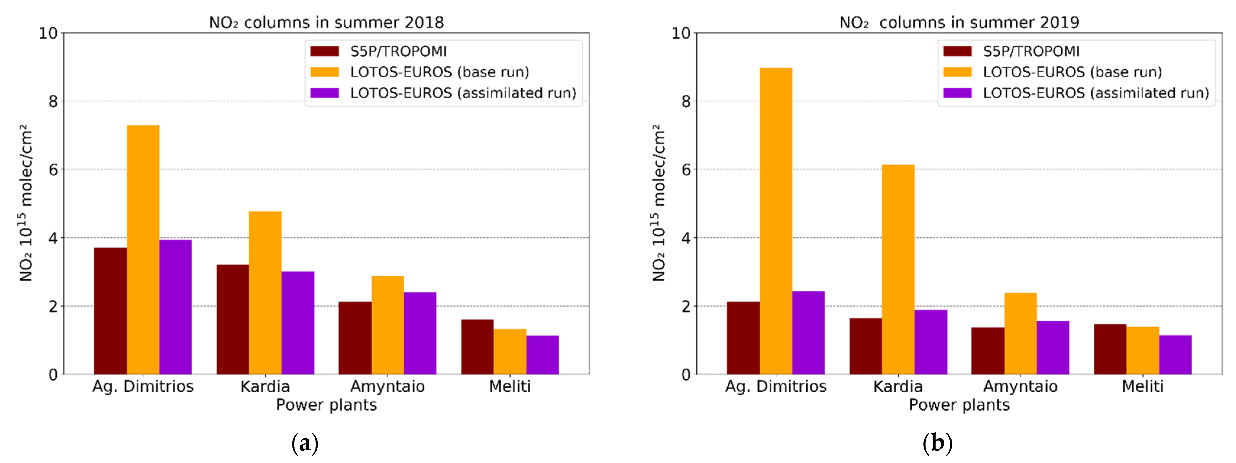
| Ag. Dimitrios | 3.70 ± 2.42 | 7.29 ± 5.14 | 3.59 | 2.11 ± 1.43 | 8.97 ± 6.17 | 6.86 |
| Kardia | 3.20 ± 2.51 | 4.75 ± 3.83 | 1.55 | 1.64 ± 0.67 | 6.13 ± 4.31 | 4.50 |
| Amyntaio | 2.13 ± 1.20 | 2.88 ± 1.90 | 0.75 | 1.37 ± 0.53 | 2.38 ± 0.93 | 1.01 |
| Meliti | 1.61 ± 0.61 | 1.33 ± 0.50 | −0.28 | 1.46 ± 0.47 | 1.40 ± 0.96 | −0.06 |
| Relative Differences | Ag. Dimitrios | Kardia | Amyntaio | Meliti |
|---|---|---|---|---|
| 2018–2015 | −38% | −27% | −1% | −11% |
| 2019–2015 | −63% | −63% | −37% | −1% |
| Air Quality Stations | Emission Sources | Seasonal Mean (μg/m3) ± std | Bias (μg/m3) | |||
|---|---|---|---|---|---|---|
| Measurements | Base Run | Assimilated | Base Run | Assimilated | ||
| Koilada | P.P. Ag. Dimitrios | 3.39 ± 2.74 | 13.92 ± 10.18 | 5.39 ± 4.65 | 10.52 | 2.00 |
| Filotas | Town of Filotas/P.P. Amyntaio | 5.38 ± 3.52 | 4.91 ± 4.46 | 3.12 ± 3.12 | −0.47 | −2.26 |
| Amyntaio | Town of Amyntaio/P.P. Amyntaio | 4.00 ± 2.25 | 7.49 ± 7.57 | 5.73 ± 6.35 | 3.49 | 1.73 |
| Meliti | Town of Meliti/P.P. Meliti/P.P. Bitola | 8.18 ± 6.46 | 6.55 ± 6.23 | 5.84 ± 6.49 | −1.63 | −2.34 |
| Florina | Town of Florina | 4.93 ± 2.45 | 6.10 ± 6.35 | 4.57 ± 5.65 | 1.17 | −0.35 |
| Relative Differences | Ag. Dimitrios | Kardia | Amyntaio | Meliti | ||||
|---|---|---|---|---|---|---|---|---|
| Energy | Emissions | Energy | Emissions | Energy | Emissions | Energy | Emissions | |
| 2018–2015 | −27% | −38% | −31% | −27% | −43% | −1% | 2% | −11% |
| 2019–2015 | −48% | −63% | −90% | −63% | −88% | −37% | −51% | −1% |
Publisher’s Note: MDPI stays neutral with regard to jurisdictional claims in published maps and institutional affiliations. |
© 2021 by the authors. Licensee MDPI, Basel, Switzerland. This article is an open access article distributed under the terms and conditions of the Creative Commons Attribution (CC BY) license (https://creativecommons.org/licenses/by/4.0/).
Share and Cite
Skoulidou, I.; Koukouli, M.-E.; Segers, A.; Manders, A.; Balis, D.; Stavrakou, T.; van Geffen, J.; Eskes, H. Changes in Power Plant NOx Emissions over Northwest Greece Using a Data Assimilation Technique. Atmosphere 2021, 12, 900. https://doi.org/10.3390/atmos12070900
Skoulidou I, Koukouli M-E, Segers A, Manders A, Balis D, Stavrakou T, van Geffen J, Eskes H. Changes in Power Plant NOx Emissions over Northwest Greece Using a Data Assimilation Technique. Atmosphere. 2021; 12(7):900. https://doi.org/10.3390/atmos12070900
Chicago/Turabian StyleSkoulidou, Ioanna, Maria-Elissavet Koukouli, Arjo Segers, Astrid Manders, Dimitris Balis, Trissevgeni Stavrakou, Jos van Geffen, and Henk Eskes. 2021. "Changes in Power Plant NOx Emissions over Northwest Greece Using a Data Assimilation Technique" Atmosphere 12, no. 7: 900. https://doi.org/10.3390/atmos12070900
APA StyleSkoulidou, I., Koukouli, M.-E., Segers, A., Manders, A., Balis, D., Stavrakou, T., van Geffen, J., & Eskes, H. (2021). Changes in Power Plant NOx Emissions over Northwest Greece Using a Data Assimilation Technique. Atmosphere, 12(7), 900. https://doi.org/10.3390/atmos12070900