A Graphics Processing Unit (GPU) Approach to Large Eddy Simulation (LES) for Transport and Contaminant Dispersion

Abstract

Recent advances in the development of large eddy simulation (LES) atmospheric models with corresponding atmospheric transport and dispersion (AT&D) modeling capabilities have made it possible to simulate short, time-averaged, single realizations of pollutant dispersion at the spatial and temporal resolution necessary for common atmospheric dispersion needs, such as designing air sampling networks, assessing pollutant sensor system performance, and characterizing the impact of airborne materials on human health. The high computational burden required to form an ensemble of single-realization dispersion solutions using an LES and coupled AT&D model has, until recently, limited its use to a few proof-of-concept studies. An example of an LES model that can meet the temporal and spatial resolution and computational requirements of these applications is the joint outdoor-indoor urban large eddy simulation (JOULES). A key enabling element within JOULES is the computationally efficient graphics processing unit (GPU)-based LES, which is on the order of 150 times faster than if the LES contaminant dispersion simulations were executed on a central processing unit (CPU) computing platform. JOULES is capable of resolving the turbulence components at a suitable scale for both open terrain and urban landscapes, e.g., owing to varying environmental conditions and a diverse building topology. In this paper, we describe the JOULES modeling system, prior efforts to validate the accuracy of its meteorological simulations, and current results from an evaluation that uses ensembles of dispersion solutions for unstable, neutral, and stable static stability conditions in an open terrain environment.

1. Introduction

The methods used to simulate outdoor dispersion of airborne materials range from simple, computationally efficient empirical approaches to complex computational fluid dynamics (CFD)-based approaches. The simplest methods use empirical formulations that utilize information on the meteorological conditions to control the corresponding dispersion behavior produced by the model. More complex CFD methods, on the other hand, are capable of resolving (explicitly or implicitly) the time-varying wind, turbulence, and dispersion patterns that drive the downwind transport and dispersion of the material. This enables the development of dispersion simulations that can reconstruct the detailed structures in the contaminant dispersion that qualitatively resembles the “single-realization” visual depictions of smoke dispersion observed in photographs. The challenge inherent with creating “single-realizations” of dispersion with a CFD model is that atmospheric measurements are typically not sufficient to adequately initialize these microscale atmospheric simulations (e.g., at spatial resolutions in the 10s of meters and timescales on the order of 1 s). To produce ensembles of “single-realization” dispersion solutions, the CFD model is initialized with the mean atmospheric conditions that can be measured and then an ensemble of uncorrelated dispersion solutions can be created by moving the release (e.g., in location and/or time) within the turbulent flow. This approach provides a distribution of dispersion solutions that can then be averaged (in time and space) to determine the mean properties of downwind dispersion analogous to the products produced by standard Gaussian plume and puff models. Alternatively, this distribution of dispersion solutions can be sampled/analyzed to understand the variance from the mean and the skewness of the distribution if present [1]. While this approach can be used to provide a wealth of information on the properties of dispersion for a given scenario, the production of ensembles of single-realization dispersion solutions is computationally expensive when compared to traditional Gaussian plume/puff and Lagrangian particle modeling techniques. The computational expense associated with producing these ensembles has, until recently, limited the use of CFD models for dispersion to research and academic applications.

Here, we introduce a large eddy simulation (LES) CFD model that has been implemented to run on a GPU computing platform and discuss the computational performance advantages provided by this GPU-LES approach. The accuracy of the dispersion solutions is critical for providing confidence in the use of this emerging technology. In this paper, we provide an illustration of an approach for validating dispersion simulations at these spatial and temporal scales. Our validation discussion includes a description of the observational data sets used to evaluate the model and the methodology used to simulate these experiments and to compare predictions to the observations. Detailed results across environmental conditions ranging from unstable to stable planetary boundary layer (PBL) conditions (i.e., daytime to nighttime) are provided. We conclude with a summary of the findings, and a brief description of the plans to extend this capability to support modeling urban environments and building interiors.

1.1. Ensemble-Average and Single-Realization Dispersion Solutions

A common simulation method for estimating the dispersion of airborne contaminants are ensemble-average approaches. These are largely empirical approaches in which the model is designed to represent the apparent stochasticity of atmospheric turbulence and its corresponding impact on downwind dispersion. Here, empirical parameters are used to describe dispersion that might have occurred over many atmospheric and dispersion conditions. When formulated for a Eulerian reference frame, these empirical parameters are used to describe airborne material dispersion relative to the mean wind direction where the rate of dispersion changes as a function of downwind distance for a given atmospheric condition. When formulated for a Lagrangian reference frame, airborne material dispersion in these tools is computed from the perspective of a hypothetical air parcel following the mean winds. The empirical parameters used to control the material spread following the flow are typically represented by a series of Gaussian puffs or individual particles. For the Lagrangian puff models, an assumption is made to represent localized concentration patterns using a Gaussian distribution, where the empirical parameters control the localized crosswind spread of the material as a function of downwind distance and atmospheric conditions [2,3]. In Lagrangian particle models, the empirical parameters are typically used to control the magnitude of particle spread within a random-walk method that redistributes the particles at each model time step [4,5]. In both approaches, there is an implicit assumption that the material concentration at each point in space and time is an ensemble average over a large number of realizations of this apparent stochastic process.

Individual realizations of dispersion can differ significantly from the ensemble-average solution, and it is typically not possible to recover specific details of a given dispersion realization from the ensemble-average statistics [6]. While ensemble-average solutions can in general provide reasonable model assessments, they have been shown to provide incorrect and misleading results, particularly for scenarios involving high-frequency data sampling, strong spatial and temporal correlations between variables, and nonlinear effects [1,7]. For example, the consequences of exposure to airborne contaminants may depend nonlinearly on the concentration, so that brief exposure to a high concentration can have greater impact than longer exposure to the same time-averaged concentration. CFD models can be used to create ensembles of what we refer to as “single-realization” dispersion solutions that use a very short time average relative to the eddy turn-over time of the eddies in the flow field. Individual uncorrelated dispersion realization ensemble members can be created in a couple of ways. One approach is to create multiple independent simulations where the model is started from slightly different initial conditions. One way to do this is by modifying the random number seed on the initial heat flux distribution that initiates the turbulence within the model. A second approach is to create uncorrelated releases by spacing a set of releases within a simulated boundary layer with spatially homogenous conditions (e.g., roughness length, heat flux, etc.). A third way this can be done is to create realizations by creating releases within a spatially and homogeneous environment at different times. The use of this approach with a CFD and dispersion model has been demonstrated to produce an ensemble of dispersion solutions that when averaged can closely replicate the dispersion solution from a Gaussian puff model that calculated dispersion based on empirical relations designed to replicate an ensemble averaged dispersion. A more detailed discussion of this can be found in Bieringer et al. [1].

The large eddy simulation (LES) modeling approach has demonstrated the ability to successfully predict unique simulations of many types of atmospheric scenarios relevant for airborne dispersion and defense analyses described above [1,6,8,9]. LES models have been developed to explicitly resolve the motions associated with the largest eddies in the atmospheric boundary layer and use parameterizations or closures to represent the small-scale turbulent eddies. The large eddies are resolved or separated from the small, unresolved eddies by filtering the governing Navier–Stokes equations in the inertial subrange, whereby the eddies smaller than the filter width are treated by a subgrid model and the eddies larger than the filter are explicitly resolved [10]. The filter size used is dependent upon the type of atmospheric conditions being modeled and the corresponding turbulence length scales involved. Air-flow solutions from LES models can be produced at spatial grid increments approaching 1 m and be solved at very short time-steps that when used to drive dispersion models (in both Lagrangian and Eulerian reference frames), can produce single-realization dispersion patterns [1,6,11,12,13,14]. When combined with an immersed boundary method (IBM) surface layer parameterization, necessary to keep the model numerically stable at the walls of the buildings, LES models have also been demonstrated to be capable of simulating the detailed winds and dispersion that occur in urban environments [15,16]. When compared to observational data, the results indicate that an LES approach has been shown to accurately represent both the mean properties of dispersion and the variance present in the observations from open terrain convective boundary layer field trials [11,12,17].

1.2. GPU-Enabled Atmospheric Computing

General purpose computing on graphics processing unit (GPGPU) hardware, hereafter referred to as a GPU, has emerged as a high-performance computing (HPC) option for a variety of applications, including scientific computing. GPUs typically have many times the number of computational cores relative to central processing unit (CPU) computers and are purpose built to solve problems in graphics shaders for the calculation of the levels for light, darkness, and color for the rendering of graphics on computer screens. Scientific computing with this technology began in the early 2000s with a demonstration using a matrix multiplication application that was shown to run considerably faster on a GPU than on a CPU [18]. Since then, programming languages and standards, such as OpenCL and Nvidia’s CUDA, provide an application programming interface that enables the use of C and C++ software to be executed on GPUs. Modern GPUs, such as the Nvidia A100, have even more densely packed computational cores (nearly 7000), and higher memory bandwidth (2 Terabytes per second) [19], which collectively enable faster computations and reduced data latency (reduced time spent waiting for data load/store processes to complete). Collectively, these characteristics enable the GPUs to significantly outperform CPUs for calculations in data-parallel applications, which require the same instruction (or calculation) to be made concurrently. Many scientific calculations, including CFD and LES calculations, fall into this data parallel paradigm.

The atmospheric science modeling community recognized the computational potential provided by the GPU in the mid to late 2000s. Early examples where the use of a GPU for an atmospheric modeling application explored the porting of computationally expensive elements of the Weather Research and Forecast (WRF) model [20] to run on a GPU. This work, commonly referred to as GPU acceleration, includes work by Michalakes and Vachharajani [21], Mielikainen et al. [22], Silva et al. [23], and Wahib and Maruyama [24]. An alternative approach that has been more recently taken by atmospheric modelers is to port the entire atmospheric model to run resident on the GPU. Examples of models that take this approach include the GPU Resident Atmospheric Simulation Program (GRASP) (previously referred to as the GPU-resident Atmospheric Large-Eddy Simulation (GALES) model) by Schalkwijk et al., 2012 [25]; Schalkwijk et al., 2015 [26]; Schalkwijk et al., 2016 [27]; the Parallelized Large Eddy Simulation Model (PALM) by Maronga et al., 2015 [28]; the MicroHH model by van Heerwaarden et al., 2017 [29] and the FastEddy model (Sauer, J. A., & Muñoz-Esparza, D. (2020) [30]. Using the CPU to handle data input and output (I/O) and moving all of the core atmospheric calculations to the GPU has been shown to provide an increase in the calculation speed of an atmospheric simulation by more than an order of magnitude over comparable calculations on CPU hardware [29].

To characterize these benefits, our team conducted benchmark LES simulations using the Weather Research and Forecast (WRF) model with LES turbulence closure [31,32] and compared the computational performance to the GRASP model. The WRF-LES and GRASP simulations used a 128 × 128 × 64 (X, Y, Z) grid with a spatial resolution of 20 m × 20 m × 17 m. The simulation used a periodic lateral boundary condition to spin up convective eddies and turbulence over a 1-h period. The WRF-LES simulation was performed on a Dell R640 running Red Hat v7.6 Linux on an Intel Xenon E5 v4, 8-core CPU, and was configured to use the distributed memory, Message Passing Interface (MPI), option. On this hardware, a 1-h WRF-LES simulation required approximately 1 h and 32 min of wall clock time. A comparable GRASP simulation was performed on an NVIDIA Tesla K40 with 2880 cores operating at 745 MHz and 12 GB of onboard fast access memory. The GRASP simulation completed in 36 s of wall clock time. This represents a GPU-LES simulation that is approximately 150 times faster than the comparable CPU-LES simulation.

The GPU-LES has substantially lower equipment costs, power consumption, cooling requirements, and physical space requirements than a CPU platform that can provide comparable simulations. Based on the benchmark described above, and assuming linear performance scaling, we estimate that a cluster of 19 Dell R640 Linux servers and a high-speed network switch would be required to match the performance of a single NVIDIA Tesla K40. Evidence on the hardware performance of the GPU vs. CPU suggests that this type of computational performance difference is a sustained characteristic of these platforms. Figure 1 shows the theoretical computational capacity and memory bandwidth benchmarks for a series of NVIDIA GPUs and Intel CPUs over the past decade [33,34]. This figure illustrates how the GPU continues to maintain a significant advantage over its Intel CPU counterpart, as measured by floating point operations per clock cycle and memory bandwidth speed, and that this advantage has continued to grow as new architecture designs are released. For reference, the NVIDIA K40 used for the performance benchmark cited above is a 2014 graphics card based on the NVIDIA Kepler architecture.

1.3. Atmospheric Dispersion Modeling on a GPU-LES Model

To form an ensemble of single-realization dispersion solutions using a LES and coupled atmospheric transport and dispersion (AT&D) model comes at a high computational expense. In spite of the computational burden that has historically been associated with LES AT&D, it has been used in a variety of studies ranging from characterizing convective boundary layers [13], the development of more accurate Lagrangian dispersion modeling through the incorporation of subgrid turbulence [11,12], and the use of dispersion ensembles for hazard prediction and sensor placement calculations [1,17]. In recent years, LES models are being increasingly used for atmospheric dispersion studies [25,26] and when implemented on GPU-based computing platforms, showed great promise for enabling a range of atmospheric boundary layer research topics and applications by significantly reducing the computational resource requirements to make the calculations [27]. Here, we present a dispersion modeling system designed to take advantage of the GPU-LES modeling technology called the joint outdoor-indoor urban large eddy simulation (JOULES). JOULES is a collection of modeling capabilities designed to calculate atmospheric conditions and corresponding airborne contaminant transport in open terrain and urban locations both inside and outside of buildings. At the core of JOULES is the GPU Resident Atmospheric Simulation Program (GRASP) described above. GRASP was originally developed to provide high-resolution simulations of clouds, winds, and turbulence and designed to be run on central processing unit (CPU) computing platforms. It was later adapted to run on GPU-based architectures by scientists at Delft University of Technology (TU Delft) and Whiffle B.V. Additional details on the origins of this model as well as information on the turbulence closures and other formulations used within the GRASP model can be found in [25,26,27].

Since its initial development, GRASP has undergone a number of evaluations to assess its ability to provide high-resolution reconstructions of atmospheric variables and short-term weather predictions. Of particular relevance to its use for atmospheric dispersion applications is the work by Schalkwijk et al. [25,26] to couple GRASP to a regional-scale atmospheric model in order to predict a continuous, year-long, three-dimensional time series of turbulence and clouds. The predictions were compared to detailed boundary layer observations collected at the Cabauw Experimental Site for Atmospheric Research (CESAR). This study included favorable comparisons between the measured and simulated power spectrum of horizontal and vertical wind speed variance across a variety of weather conditions and temporal scales.

2. Materials and Methods

In this section, we describe the implication of coupling JOULES with an AT&D model, which solves for the advection and diffusion of a passive scalar (i.e., a neutrally buoyant airborne tracer). Our study evaluates the accuracy of the GPU-LES dispersion solutions produced by this model over flat open terrain. The evaluation was performed using data from three separate dispersion experiments, with atmospheric conditions ranging from unstable daytime “convective” PBLs, to stable environments that typically occur at night. This section describes the observational data used in the model evaluation, the approach used to develop the ensembles of dispersion solutions, the analysis methodology, and the metrics used to compare the simulations to the observations.

2.1. Observational Data

This study uses data from three dispersion experiments, representing open terrain environments under unstable, neutral, and stable conditions. The observations during unstable or “convective” conditions were taken from the classic convective water tank experiments conducted by Willis and Deardorff [35], and two outdoor atmospheric trials, Project Prairie Grass [36,37], and the COnvective Diffusion Observed by Remote Sensor (CONDORS) experiments [38,39,40]. Collectively, these three experiments provide data from trials representing both near-surface airborne tracer releases and observations of material concentrations at the surface and aloft. Since vertical dispersion is less significant in stable conditions, near-surface observations from Project Prairie Grass were used to assess our implementation for neutral and stable simulations. The following subsections describe these data.

2.1.1. Willis and Deardorff Water Tank Experiments

Historically, the development of ensembles of dispersion realizations from outdoor dispersion measurements has been difficult to construct because the atmospheric conditions in which the measurements are taken typically do not repeat with sufficient consistency or frequency during the experiments. Laboratory experiments are one way of addressing this challenge and have been demonstrated to provide comprehensive ensembles of dispersion for repeatable conditions. In the 1970s and 1980s, Willis and Deardorff conducted a series of water-tank experiments, to measure the temperature, heat flux, wind velocity, and fluctuations in temperature and velocity in a convectively forced fluid [35]. They later extended these experiments to include dispersion in the convective boundary layer [41]. These observations, and a series of numerical simulations enabled the characterization of dispersion in the convective atmospheric boundary layer, and showed how the large variability in concentration measurements observed in convective boundary layers can be explained by the location of the release relative to the updrafts and downdrafts [42,43].

This work demonstrated that an ensemble of dispersion realizations is typically needed to characterize the statistical properties of dispersion in convective boundary layers. Later experiments measured crosswind-integrated concentration as a function of the downstream distance from the source. This led to a further extension of these earlier convective water tank experiments, where additional observational experiments were designed to produce ensembles of dispersion solutions [41,42,43] (including measurements of crosswind integrated concentrations as a function of the downstream distance from the source for a series of near-surface and elevated releases. The Willis and Deardorff observations have been used extensively to understand the convective boundary layer and in a variety of model evaluation studies [11,12,42,43] involving LES models. In this study, data from the water tank experiment were used in the assessments of the GPU-LES model simulations of downwind dispersion at the surface and aloft during convective conditions.

2.1.2. Project Prairie Grass Experiment

Project Prairie Grass [36] is a classic outdoor atmospheric dispersion field trial that has been widely used to understand the properties of atmospheric dispersion from near surface releases. Briefly, the experiment featured a series of 10-min continuous sulfur dioxide (SO₂) releases from a point 0.46 m above the ground. Downwind concentration measurements were made along five semi-circular arcs, located 50, 100, 200, 400, and 800 m from the release, at spacings of 2° for the four innermost arcs, and at 1° for the 800 m arc. Surface-based samplers collected 10-min integrated concentration measurements. The mean winds were measured at 8 heights, from 0.125 m to 16 m. The micro-meteorological information (friction velocity ($u_{*}$) and Obukhov length (L)) were determined by fitting the friction velocity and temperature measurements to the tower data. Approximately 70 releases were conducted, and data collected across a range of atmospheric stability regimes. In this study, data from the Prairie Grass experiment were used in the assessments of near-surface GPU-LES dispersion model simulations for unstable, neutral, and stable boundary layer conditions. The Project Prairie Grass data were obtained from Arhus University, Denmark [37]. We refer the reader to [36] for a full description of the experiment.

2.1.3. COnvective Diffusion Observed by Remote Sensors (CONDORS) Experiment

The COnvective Diffusion Observed by Remote Sensors (CONDORS) experiments measured both near-surface and vertical dispersion, extending to the full depth of the atmospheric boundary layer [38,39,40]. Measurements aloft included rawinsondes released near the time of the tracer experiments, acoustic sounders, and observations from a 300-m tower, which enabled estimates of the mixing layer depth, heat, and momentum fluxes. The trials used three tracers (oil fog, chaff, and a passive gas), in daytime releases near Erie, Colorado during August and September. Concentration measurements were collected by samplers at the surface, and with lidar and radar aloft. Twenty-six hours of data were collected across 12 separate mid-day periods. Of these data, over 11 h of data were processed into 29- to 60-min averaging periods during conditions where the convective boundary layer or mixed layer depth normalized by the Obukhov length (z_i/L) ranged from 24 (moderately unstable) to 1125 (extremely unstable) [38]. Obukhov length is defined as:

$$L=-u_{*}^3{T}_a/\left(kg\overline{w’\theta {’}_0}\right)$$

(1)

where $u_{*}$ is the surface friction velocity, $T_a$ is the ambient temperature, $k$ is the von Kármán constant ($k$ = 0.4), $g$ is the gravitational acceleration, and $\overline{w’\theta {’}_0}$ is the surface kinematic heat flux. This experiment provides a comprehensive set of measurements of crosswind-integrated concentration, lateral dispersion, plume height, and vertical dispersion. Data from the CONDORS experiment were used in the unstable boundary layer evaluations of the GPU-LES model dispersion at both the surface and aloft.

2.2. Categorization of the Observations

For each of the categories of static stability, we combined dispersion measurements from a combination of observations collected at multiple distances downwind from the release location and from a variety of individual trials conducted during similar weather conditions. Combining the observational data in this way enabled us to then compare both the mean and spread of the full distribution of observations to the model simulations. Taken together, the water tank, Prairie Grass, and CONDORS experiments cover a range of weather and stability conditions, near-surface and above-surface data, and distances downwind from the release location. Broadly, Prairie Grass provides near-surface dispersion estimates for unstable, neutral, and stable boundary layer conditions. For unstable boundary layers, these are supplemented by the Willis and Deardorff water tank and CONDORS data for both near-surface and vertical dispersion, including crosswind-integrated concentration, plume height, and lateral and vertical dispersion.

In order to synthesize complete datasets against which to evaluate our GPU-LES model, we organized the data around elements of the Pasquill–Gifford stability categories [44,45]. We chose to represent dispersion in convective (unstable), neutral, weakly stable, moderately stable, and strongly stable conditions, based on the ranges of the Obukhov length that have been correlated to these stability categories [46,47].

Table 1. Obukhov values used to define stability categories for the GPU-LES evaluation.

Stability	L (m)
Unstable	<−2
Neutral stability	>75
Slightly Stable	35 to 75
Moderately Stable	8 to 35
Extremely Stable	1 to 8

lists the Obukhov ranges used to select specific trials from the Project Prairie Grass and CONDORS data sets. To the extent possible, care was taken to group measurements taken under similar weather conditions. Specific trials selected by these criteria included:

• The convective water tank experimental data from Case 1 in Willis and Deardorff [26], comprising data from seven experimental trials;
• All the surface-based releases of oil and chaff, for eight releases and five locations, in the CONDORS experiment;
• Seven Project Prairie Grass trials—Trials 7, 8, 10, 16, 25, 44, and 51.

Table 2. The mean environmental conditions of the observational data used in the evaluation.

Stability	Number of Trials	U @ 1m (m s−1)	$$\begin{gathered} {\mathit{u}}_{*} \\ \left(\mathbf{m}\mathbf{s}{-}^1\right) \end{gathered}$$	Heat Flux (W m−2)	T (°C)	θ (K)	$$\begin{gathered} {\mathit{w}}_{*} \\ \left(\mathbf{m}\mathbf{s}{-}^1\right) \end{gathered}$$	L (m)
Unstable	47	4.054	0.331	200.517	28.96	307.10	1.613	−18.33
Neutral stability	12	4.84	0.38	−29.39	22.33	300.36	−0.54	167.25
Slightly Stable	7	2.74	0.21	−25.94	22.15	300.19	−0.50	54.20
Moderately Stable	6	2.21	0.16	−22.07	21.73	299.68	−0.49	18.91
Extremely Stable	9	1.24	0.07	−10.74	19.03	297.13	−0.36	4.29

gives details on the 81 individual trials distributed across the four categories and the corresponding mean atmospheric properties for each category.

2.3. Scaling Methodology

In addition to their water tank experiments, Willis and Deardorff [26] also introduced methods for scaling dispersion measurements. Their approach acknowledges that dispersion in the PBL depends primarily on the time over which the fluid disperses through the media. Their initial work considered highly convective PBLs, where non-dimensional scaling factors were derived using the convective boundary layer depth, $z_i$, and the convective velocity scale, $w_{*}={\left(g\overline{w’\theta {’}_o}{z}_i/T_a\right)}^{\frac{1}{3}}$. They further defined the turbulence time scale, or eddy-turnover time, as $z_i/w_{*}$. In the along-wind direction, they recognized that, because dispersion in the PBL is a function of time, downwind distance, $X$, from the source for convective conditions can be scaled as:

$$X=\frac{w_{*}x}{U{z}_i}$$

(2)

where $x$ is the distance downwind of the release location, and $U$ is the average PBL wind speed. Willis and Deardorff [26] also suggested a dimensionless parameter for the crosswind integrated concentration (CWIC or $C^y$), defined as $C^y={{\displaystyle \int }}_{-\infty }^{\infty }C\left(x,y,z\right)dy$. To do so, they scaled CWIC by the concentration that would be present in a uniformly mixed PBL, well downwind of the release. This uniformly mixed concentration is $Q/U{z}_i$ where $Q$ is the mass-release rate. Based on this approach, a normalized dimensionless CWIC can be calculated as:

$$Normalized CWIC=\frac{C^{y}U{z}_i}{Q}$$

(3)

This approach was first used by Willis and Deardorff [35] to visualize the dispersion measurements from their convective water tank experiments. Our work here leverages these methodologies and in particular plots of CWIC like Figures 8 and 9 from Willis and Deardorff [35] that depict measurements with a non-dimensional mean CWIC from the water tank data that was plotted as a function of the scaled downwind distance $X$ and height.

Since its introduction, this scaling approach has been extended and adapted for use in atmospheric dispersion applications that range from interpreting observational data [48] to the development of empirical models [49,50] and the evaluation of dispersion models [11,12]. Here, we used this scaling approach to combine observations taken at different times from a single experiment, and observations taken from different experiments, into a collection of measurements that represent dispersion in each stability class. Similar methods were used by Weil et al. [11,12] for unstable conditions, and Venkatram et al. [51] for neutral and stable conditions. The scaling used in this study and by Weil et al. [11,12] for the convective cases closely follows the approach found in [35]. For evaluating plume height, and vertical and lateral dispersion, we also followed the Weil et al. [11,12] approach of normalizing the results by $z_i$.

The downwind distance scaling method used in this evaluation for the neutral and stable static stability conditions follows the approach published in [50]. The Venkatram et al. [50] scaling differs slightly from that of Willis and Deardorff [35], normalizing the downwind distance using:

$$X=\frac{x}{\left|L\right|}$$

(4)

where $\left|L\right|$ is the absolute value of the Obukhov length from Equation (1). Because the convective scale velocity of neutral-to-stable cases would be negative, we instead use a scaling factor that utilizes friction velocity and Obukhov length. For neutral and stable scenarios, normalized CWIC is calculated using the following relationship:

$$Normalized CWIC= \frac{C^y{u}_{*}L}{Q}$$

(5)

The scaling parameters, as described above, are applied to all of the point-location observations used in this evaluation. The same relationships are applied to the simulations enabling a comparison with the observations.

2.4. GPU-LES Model Simulations

The development of the GPU-LES dispersion simulations involved a two-step process. The first step was the design and execution of the atmospheric simulation. Five configurations, corresponding to the stability categories defined in Table 1 and Table 2, were developed. The unstable configuration was based on the specifications of Weil et al. [11,12]. The neutral and stable configurations required finer spatial resolution, and a different approach for establishing the desired stability conditions. To achieve a simulation with the desired Obukhov length, we set the roughness length, heat flux, temperature, and initial convective boundary layer depth to values representative of the environmental conditions in the ensemble of field trials. Next, we adjusted the geostrophic wind (U_g and V_g) until the Obukhov length matched the observations within the category.

Table 3. The JOULES GPU-LES model configuration parameters.

Simulation Category	Grid Points (nx,ny,nz)	Model Resolution (Hor,Vert) (m)	U (m/s)	Ug (m/s)	Vg (m/s)	Heat Flux (W/m2)	zi (m)	L (m)
Unstable	(192,192,96)	(52.1,20.8)	2.8	2.8	−1.5	240	1000	−11.5
Neutral stability	(256,256,64)	(6.25,6.25)	8	8	−5.5	−10	190	372.2
Slightly Stable	(256,256,64)	(6.25,6.25)	4	3.5	−4.5	−10	116	47.6
Moderately Stable	(256,256,64)	(6.25,6.25)	4	3.2	−4.2	−10	103	28.9
Extremely Stable	(256,256,64)	(6.25,6.25)	3	2.5	−2.5	−10	78	7.6

provides details on the model configurations and initial conditions (e.g., domain size, spatial resolutions, and core meteorological parameters). The wind speeds in Table 3 are the initial values (i.e., at the model start time) for the entire PBL. The turbulent PBL simulation is first spun up for 60 min from a cold start using cyclic (i.e., periodic) lateral boundary conditions. Figure 2 shows sample horizontal and vertical cross-sections of vertical velocity after the spin-up of a convective PBL simulation over a 2 km × 2 km × 1.0 km domain. Following the initial spin-up, we then began the tracer release, allowing the tracer mass to reach steady state. This required another 60 min of simulated time. Hence, we did not use meteorological or dispersion results from the first 120 min of the simulations. Our development here emphasized model selections that aided in separating model calibration to the experiment conditions from model calibration to the resulting data.

The second step in developing dispersion simulation data for this evaluation is a process we used to develop an ensemble of uncorrelated dispersion solutions. Once the GPU-LES model has spun up the turbulence and corresponding dispersion to a quasi-steady state, we calculated the model evaluation metrics. A continuous set of values in the along-wind direction were computed for each of the evaluation metrics. The calculations used a 10-min average or integrated value, depending on the metric in question. Individual uncorrelated realizations of the dispersion patterns, following the methodology used in [12], were created by varying a combination of the source location and the start time of the release. For example, Figure 3 depicts the predicted near-surface concentrations from five uncorrelated simulations. It illustrates the type of variability in the dispersion patterns that can be created within a convective PBL simulation using this methodology. Because the GPU-LES model runs quickly, we were able to generate an ensemble of 130 realizations that we believe described the unstable PBL dispersion comprehensively and do so in approximately two hours of wall-clock time for these experiments. Subsequently, for the neutral and stable simulations, we reverted to using 30 realizations per ensemble, as was done in [12], and we found suitable for our comparisons. The model evaluation metrics were then computed for each ensemble member, using the sampling characteristics of the field program. This enabled us to create a comprehensive distribution of model evaluation metrics that captured the range of dispersion patterns associated with how the airborne material release responds to the winds and turbulence in the PBL.

3. Results

We assessed the suitability of the GPU-LES model to simulate dispersion in the PBL by comparing the plume height normalized by PBL height, vertical profiles of CWIC, downwind surface-based CWIC, surface crosswind dispersion, and vertical dispersion to comparable dispersion metrics computed from observations. Calculations of the metrics computed from observations are represented by symbols/markers in the forthcoming figures. Calculations of the metrics for a single dispersion realization from the GPU-LES model simulations are represented by either grey lines or blue dots and are plotted on the figure to illustrate the distribution of solutions. The following sections present results comparing the JOULES GPU-LES model predictions to observational data and are organized by stability category as described in Table 1.

3.1. Unstable PBL Comparison

The observational data sets used for the unstable PBL evaluation were from the Willis and Deardorff [35] water-tank, the Project Prairie Grass, and CONDORS experiments. The crosswind integrated concentration was computed from the release location to a downwind distance of 9750 m, for the full vertical depth of the simulation (2000 m). Figure 4 shows the CWIC calculation from the unstable GPU-LES dispersion solution. Qualitatively, the results closely match the measurements illustrated in Figure 8 from the Willis and Deardorff [35] experiment for scaled downwind distances less than three. Overall, the GPU-LES dispersion solution shows strong qualitative agreement with the Willis and Deardorff [35] observations, notably the near surface concentration minimum that occurs between a downwind distance of ~1 to 3. Because the GPU-LES simulation extends beyond the downwind distance measured by Willis and Deardorff, we are able to predict an increase in average CWIC near surface extending out to a scaled downwind distance of X = ~5.

Figure 5 shows a quantitative comparison of the GPU-LES CWIC solution with the Willis and Deardorff [35] data. The figure illustrates how CWIC varies with height, out to a scaled downwind distance of approximately 3 from the release location. Past X = 3, the CWIC value shows unity up to the height of the boundary layer. It shows promising agreement between the ensemble mean of CWIC from the GPU-LES model (black line) and the measured vertical profiles of CWIC from the water tank experiments (black dots).

Surface measurements for calculating CWIC were available from the Project Prairie Grass and CONDORS experiments. Figure 6 compared surface CWIC measurements (represented by the black circles, dots, squares, and stars) with calculations from 130 GPU-LES realizations (represented by the small blue dots). The green line denotes a calculation of CWIC using surface layer similarity (SLS) theory [51]. At locations nearest the source, the LES model under predicts CWIC compared to SLS theory and Prairie Grass data. This is due to the resolution of the computational grid. Near the source, the tracer is immediately dispersed uniformly throughout each grid cell, making the model over-dispersive at this location. The underprediction near the source can be addressed (when required) by decreasing the volume of the grid cells (i.e., increasing the spatial resolution), or through the use of a Lagrangian particle dispersion model (LPDM). Figure 6 shows that, except very near to the source, the simulations of surface-based normalized CWIC show promising agreement with the measurements from the field trials. The figure also illustrates how the spread in the observations and model simulations vary as a function of the scaled downwind distance from the source. Notably, both show the pattern of smaller spread near the source location, an increase in spread near a scaled downwind distance of one, and then a collapse of the spread to a CWIC value near one further downwind as the material becomes well-mixed in the PBL.

Figure 7 compared lateral or horizontal crosswind dispersion, computed from surface observations from both the Project Prairie Grass and CONDORS experiments, and corresponding calculations of lateral dispersion from the GPU-LES model. Here, again, there is fair agreement between the observations and the mean lateral dispersion from the ensemble of simulations. A majority of observations fall within the ensemble distribution, and the slope of the increase in plume spread with distance is well aligned with the observations. However, the mean of the ensemble appears to be slightly below the observations, including the formulation fit to the data by Briggs [48], for scaled downwind distances greater than approximately 0.1.

In Figure 8 we illustrate the vertical dispersion results. For this metric, the mean of the ensemble aligns well with the observations, and the spread of the ensemble corresponds nicely to the spread observed in the CONDORS data. This metric also demonstrates that the GPU-LES dispersion model exhibits the expected increase in vertical dispersion as the scaled downwind distance increases. Finally, it appears to correctly capture the properties in the vertical dispersion observations, where normalized vertical dispersion stabilizes at scaled downwind distances greater than one.

Figure 9 shows the normalized average plume height, $\overline{z_p}$, as a function of the scaled downwind distance. Excluding outlier observations during sampling periods 32 and 33 (pds 32,33) in the CONDORS field trials, noted by Briggs [49], there is good agreement between the CONDORS observations of $\overline{z_p}$ and the dispersion realizations. The average value of $\overline{z_p}$ from the ensemble of simulations (black line) is near the center of the scatter of observations. The ensemble of the plume height calculations presents little variability near the release location and far downwind of the release, but a greater range of results at scaled downwind distances between X = 0.75 and 2.5. This pattern in the ensemble spread agrees closely with the scatter observed in the CONDORS observations. It also matches expectations based on the characteristics of dispersion in a strongly convective PBL environment.

3.2. Neutral and Stable PBL Comparison

Data from the Project Prairie Grass field experiment were also used to evaluate the dispersion solutions from the GPU-LES dispersion simulations for neutral and stable PBL conditions. Our selection criteria identified surface concentration data from 34 trials for use in the model evaluation. As described above, in order to account for variability of dispersion conditions within this range of stability categories, we categorized these data into four distinct subsets; see Table 1. Surface CWIC and lateral dispersion results are provided for each category.

3.2.1. Neutral PBL Comparison

Figure 10 shows a vertical cross-section of normalized CWIC as a function of the downwind distance calculated from the ensemble of 30 neutral GPU-LES dispersion simulations with an Obukhov length of ~372 m. It illustrates that for the neutral condition simulations, the airborne materials from a surface release mix up to about half the depth of the PBL (~95m). In Figure 11, the calculation of CWIC from the GPU-LES model was compared to calculations of CWIC from the surface observations from the Prairie Grass experiment, where the Obukhov length during the experiment was greater than 75 m. This figure shows good agreement between the CWIC observations (black dots) and the values computed from the GPU-LES simulations (blue dots). The red line depicts the ensemble average of the CWIC simulations. Note that the slope of this line matches the slope of the observations. The figure also indicates that the width of the distribution from the ensemble of simulations is very consistent with the scatter suggested by the observations.

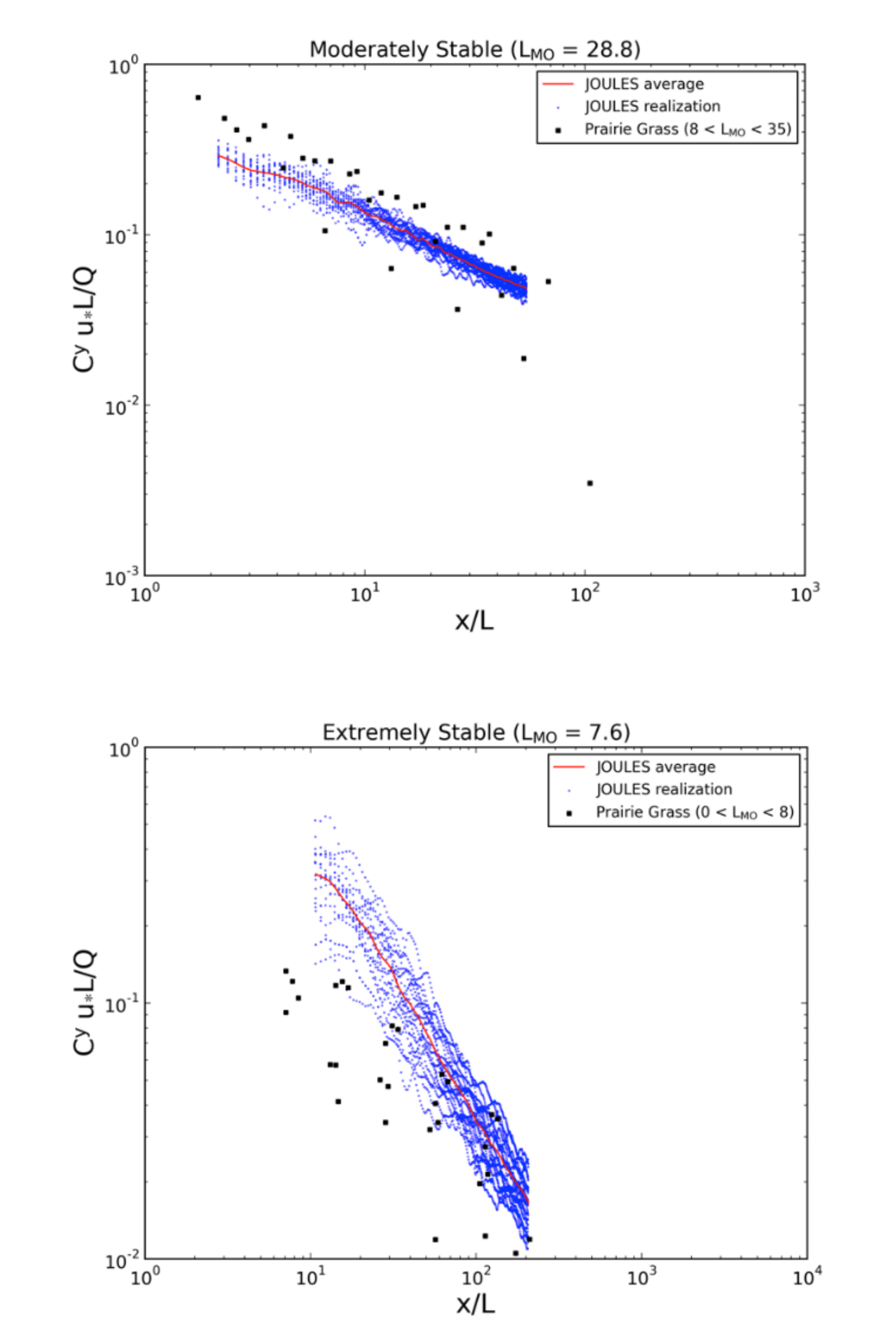
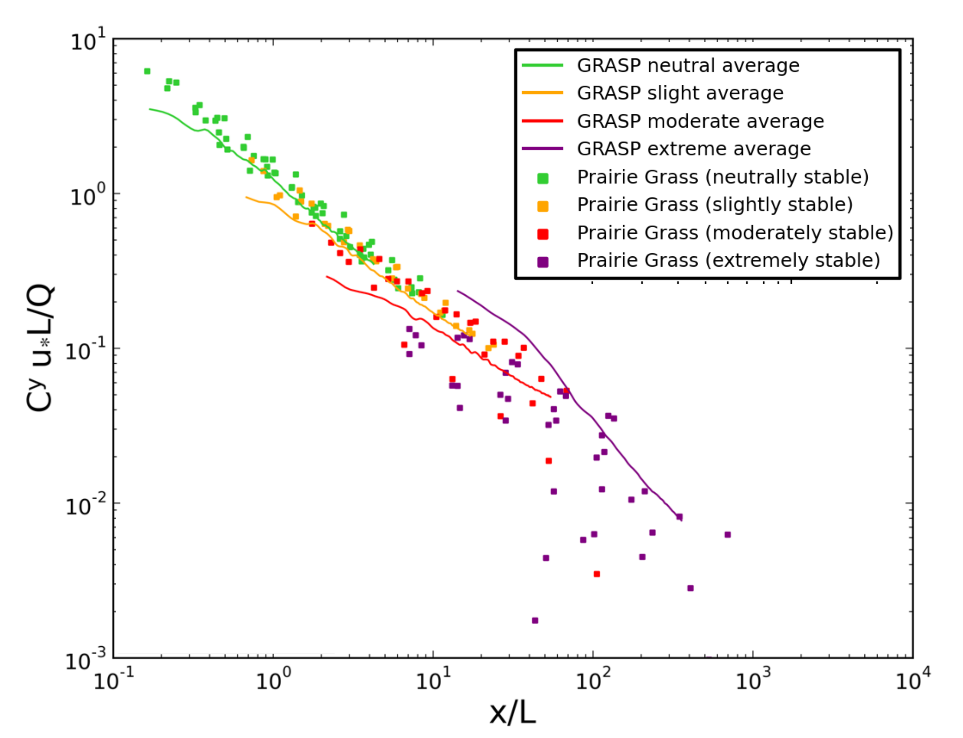
3.2.2. Stable PBL Comparison

Similar calculations were made for the simulations produced for the slightly, moderately, and extremely stable PBL conditions. Figure 12 depicts the vertical cross-sections of CWIC for each and illustrates how the simulated CWIC values vary as the environmental conditions become more stable. As expected, the depth to which the airborne materials from a surface release are mixed decreases as the static stability increases (approximately 62, 41, and 31 m for the weakly, moderately, and extremely stable conditions, respectively). This results in higher concentrations being seen further downwind of the release location as the atmosphere becomes more stable. The data from these three stability categories were also directly compared to normalized CWIC calculations made using Project Prairie Grass observations. The results, summarized in Figure 13, show good agreement between the model and observations for the weakly and moderately stable conditions. There was considerably more scatter in the CWIC data computed from the ensemble of extremely stable observations and the ensemble average of the extremely stable GPU-LES CWIC simulations was on the high end of the pattern of observations (though still within the range of the scatter). This suggests that the turbulence is much lower in our GPU-LES simulation than what was present in the experimental data and that we do not have a sufficient understanding of the sources of turbulence in these very stable cases to incorporate it into the simulation.

In Figure 14, results from the neutral through extremely stable cases are plotted to depict the collective information on model accuracy for this range of stabilities. These results, and the results shown earlier for the convective PBL environments, indicate that the GPU-LES modeling system may be able to be configured from first principal parameters to provide ensembles of single-realization dispersion solutions that are representative of this range of environmental conditions.

4. Discussion and Conclusions

A research goal for developing our GPU-LES approach, JOULES, is to design a system for computing single-realizations of detailed, coupled urban (outdoor-indoor) contaminant dispersion. To describe the variability inherent in the atmospheric and urban conditions, our design required that that each simulation is completed quickly so that we could generate many realizations, all equally probable. A resulting capability would allow us to compute mass-conserving transport in a complete urban setting for various applications, many which cannot be analyzed using ensemble-averaging methods. The capability also allows us to derive synthetic data to test the suitability of existing operational tools.

Here, we present the evaluation of the JOULES dispersion solutions for open terrain environments. These tests are critical for many applications. It is also essential before testing it for more complex urban settings. This study used observational data from three field trials, following peer-reviewed methods and evaluation metrics that have been extended to evaluate the GPU-LES dispersion model’s suitability and promise across a range of environmental conditions, including convective (daytime) and extremely stable (nighttime) conditions. The open terrain convective comparisons showed very close agreement, both at the surface and aloft, for surface-based releases across this range of stability regimes. The simulations and performance metrics also closely match the performance of the Lagrangian particle dispersion model (LPDM) and National Center for Atmospheric Research (NCAR) LES model published in [12] for convective conditions.

This study moved beyond the work presented by Weil et al. [12] and examined the accuracy of dispersion simulations for neutral and stable conditions. JOULES also performed well for the neutral, weakly, and moderately stable cases when compared to surface observations from Project Prairie Grass. While there was some agreement between the dispersion simulations and observation for the extremely stable cases, the normalized CWIC calculations from JOULES were on the high end of the scatter in the observations.

The atmospheric conditions and corresponding dispersion solutions can be produced by configuring first principle PBL parameters in the model to produce a simulated environment across static stability scenarios that range from unstable convective to moderately stable conditions. The results of this model evaluation study suggest that JOULES can produce very promising atmospheric dispersion solutions for open-terrain homogeneous environments. Furthermore, the GPU implementation has been demonstrated to enable simulations to run over 150 times faster than comparable CPU-based LES implementations. This advancement significantly reduces the computational costs associated with developing microscale atmospheric and dispersion simulations and now makes it feasible to produce ensembles of single-realization dispersion solutions that are necessary in a variety of airborne dispersion and defense analyses [1,8,9].

In future work, we plan to implement a simulation capability for urban interiors. Such efforts require deciding on appropriate physics-based models and improving computational performance to allow for even larger simulation domains, terrains, and non-homogeneous land covers.

References

1. Bieringer, P.E.; Annunzio, A.J.; Platt, N.; Bieberbach, G.; Hannan, J. Contrasting the use of single-realization versus ensemble-average atmospheric dispersion solutions for chemical and biological defense analyses. J. Appl. Meteor. Climatol. 2014, 53, 1399–1415. [Google Scholar] [CrossRef]
2. Bass, A. Modelling long range transport and diffusion. In Proceedings of the 2nd Joint Conference on Applications of Air Pollution Meteorology, New Orleans, LA, USA, 24–27 March 1980; pp. 193–215. [Google Scholar]
3. Sykes, R.I.; Parker, S.; Henn, D.; Chowdhury, B. SCIPUFF Version 3.0 Technical Documentation; Sage Management: Princeton, NJ, USA, 2016; 403p. [Google Scholar]
4. Thomson, D.J. Criteria for the selection of stochastic models of particle trajectories in turbulent flows. J. Fluid Mech. 1987, 180, 529–556. [Google Scholar] [CrossRef]
5. Wilson, J.D.; Sawford, B.L. Review of Lagrangian stochastic models for trajectories in the turbulent atmosphere. Bound.-Layer Meteor. 1996, 78, 191–220. [Google Scholar] [CrossRef]
6. Haupt, S.E.; Annunzio, A.J.; Schmehl, K.J. Evolving turbulence realizations of atmospheric flow. Bound.-Layer Meteorol. 2013, 149, 197–217. [Google Scholar] [CrossRef]
7. Gunatilaka, A.; Skvortsov, A.; Gailis, R. A review of toxicity models for realistic atmospheric applications. Atmos. Environ. 2014, 84, 230–243. [Google Scholar] [CrossRef]
8. Bieberbach, G.; Bieringer, P.E.; Cabell, R.; Hurst, J.; Weil, J.; Wyszogrodzki, A.; Hannan, J. A Framework for Developing Synthetic Chemical and Biological Agent Release Data Sets. In Proceedings of the 13th International Conference on Harmonisation within Atmospheric Dispersion Modeling for Regulatory Purposes, Paris, France, 1–4 June 2010. [Google Scholar]
9. Platt, N.; DeRiggi, D.; Warner, S.; Bieringer, P.E.; Bieberbach, G.; Wyszogrodzki, A.; Weil, J. Method for comparison of large eddy simulation generated wind fluctuations with short-range observations. Int. J. Environ. Pollut. 2012, 48, 22–30. [Google Scholar] [CrossRef]
10. Wyngaard, J.C. Turbulence in the Atmosphere; Cambridge University Press: Cambridge, UK, 2010; 393p. [Google Scholar]
11. Weil, J.C.; Sullivan, P.P.; Moeng, C.H. The use of large-eddy simulations in Lagrangian particle dispersion models. J. Atmos. Sci. 2004, 61, 2877–2887. [Google Scholar] [CrossRef]
12. Weil, J.C.; Sullivan, P.P.; Moeng, C.H. Statistical variability of dispersion in the convective boundary layer: Ensembles of simulations and observations. Bound.-Layer Meteorol. 2012, 145, 185–210. [Google Scholar] [CrossRef]
13. Henn, D.S.; Sykes, R.I. Large-eddy simulation of dispersion in the convective boundary layer. Atmos. Environ. 1992, 26a, 3145–3159. [Google Scholar] [CrossRef]
14. Caulton, D.R.; Li, Q.; Bou-Zeid, E.; Fitts, J.P.; Golston, L.M.; Pan, D.; Lu, J.; Lane, H.M.; Buchholz, B.; Guo, X.; et al. Quantifying uncertainties from mobile-laboratory-derived emissions of well pads using inverse Gaussian methods. Atmos. Chem. Phys. 2018, 18, 15145–15168. [Google Scholar] [CrossRef] [Green Version]
15. Lundquist, K.A.; Chow, F.K.; Lundquist, J.K. An immersed boundary method enabling large-eddy simulations of flow over complex terrain in the WRF model. Mon. Weather. Rev. 2012, 140, 3936–3955. [Google Scholar] [CrossRef]
16. Tomas, J.M.; Eisma, H.E.; Pourquie, M.J.B.M.; Eisinga, G.E.; Jonker, H.J.J.; Westerweel, J. Pollutant Dispersion in Boundary Layers Exposed to Rural-to-Urban Transitions: Varying the Spanwise Length Scale of the Roughness. Bound. Layer Meteorol. 2017, 163, 225–251. [Google Scholar] [CrossRef] [Green Version]
17. Bieringer, P.E.; Piña, A.J.; Sohn, M.D.; Jonker, H.J.J.; Bieberbach, G., Jr.; Lorenzetti, D.M.; Fry, R.N., Jr. Large Eddy Simulation (LES) Based System for Producing Coupled Urban and Indoor Airborne Contaminant Transport and Dispersion Solutions. In Proceedings of the 18th International Conference on Harmonisation within Atmospheric Dispersion Modeling for Regulatory Purposes, Bologna, Italy, 9–12 October 2017. [Google Scholar]
18. Du, P.; Weber, R.; Luszczek, P.; Tomov, S.; Peterson, G.; Dongarra, J. From CUDA to OpenCL: Towards a performance-portable solution for multi-platform GPU programming. Parallel Comput. 2012, 38, 391–407. [Google Scholar] [CrossRef] [Green Version]
19. NVIDIA Corporation. Design and Visualization. Available online: https://www.nvidia.com/en-us/data-center/a100/ (accessed on 13 June 2021).
20. Skamarock, W.C.; Klemp, J.B. A time-split nonhydrostatic atmospheric model for weather research and forecasting applications. J. Comput. Phys. 2008, 227, 3465–3485. [Google Scholar] [CrossRef]
21. Michalakes, J.; Vachharajani, M. GPU acceleration of numerical weather prediction. Parallel Process. Lett. 2008, 18, 531–548. [Google Scholar] [CrossRef] [Green Version]
22. Mielikainen, J.; Huang, B.; Huang, H.L.A.; Goldberg, M.D. Improved GPU/CUDA based parallel weather and research forecast (WRF) single moment 5-class (WSM5) cloud microphysics. IEEE J. Sel. Top. Appl. Earth Obs. Remote. Sens. 2012, 5, 1256–1265. [Google Scholar] [CrossRef]
23. Silva, J.P.; Hagopian, J.; Burdiat, M.; Dufrechou, E.; Pedemonte, M.; Gutiérrez, A.; Ezzatti, P. Another step to the full GPU implementation of the weather research and forecasting model. J. Supercomput. 2014, 70, 746–755. [Google Scholar] [CrossRef]
24. Wahib, M.; Maruyama, N. Highly optimized full GPU-acceleration of non-hydrostatic weather model SCALE-LES. In Proceedings of the 2013 IEEE International Conference on Cluster Computing (CLUSTER), Indianapolis, IN, USA, 23–24 September 2013; pp. 1–8. [Google Scholar]
25. Schalkwijk, J.; Griffith, E.J.; Post, F.H.; Jonker, H.J.J. High-performance simulations of turbulent clouds on a desktop PC: Exploiting the GPU. Bull. Am. Meteorol. 2012, 93, 307–314. [Google Scholar] [CrossRef]
26. Schalkwijk, J.; Jonker, H.J.J.; Siebesma, A.P.; Bosveld, F.C. A year-long large-eddy simulation of the weather over Cabauw: An overview. Mon. Weather Rev. 2015, 143, 828–844. [Google Scholar] [CrossRef] [Green Version]
27. Schalkwijk, J.; Jonker, H.J.J.; Siebesma, A.P. An Investigation of the Eddy-Covariance Flux Imbalance in a Year-Long Large-Eddy Simulation of the Weather
at Cabauw. Bound.-Layer Meteorol. 2016, 160, 17–39. [Google Scholar] [CrossRef] [Green Version]
28. Maronga, B.; Gryschka, M.; Heinze, R.; Hoffmann, F.; Kanani-Sưhring, F.; Keck, M.; Raasch, S. The Parallelized Large-Eddy Simulation Model (PALM) version 4.0 for atmospheric and oceanic flows: Model formulation, recent developments, and future perspectives. Geosci. Model Dev. Discuss. 2015, 8, 1539–1637. [Google Scholar]
29. Van Heerwaarden, C.; Van Stratum, B.J.; Heus, T.; Gibbs, J.A.; Fedorovich, E.; Mellado, J.P. MicroHH 1.0: A computational fluid dynamics code for direct numerical simulation and large-eddy simulation of atmospheric boundary layer flows. Geosci. Model Dev. 2017, 3145–3165. [Google Scholar] [CrossRef] [Green Version]
30. Sauer, J.A.; Muñoz-Esparza, D. The FastEddy® resident-GPU accelerated large-eddy simulation framework: Model formulation, dynamical-core validation and performance benchmarks. J. Adv. Model. Earth Syst. 2020, 12, e2020MS002100. [Google Scholar] [CrossRef]
31. Moeng, C.H.; Dudhia, J.; Klemp, J.; Sullivan, P. Examining two-way grid nesting for large eddy simulation of PBL using the WRF model. Mon. Weather. Rev. 2007, 135, 2295–2311. [Google Scholar] [CrossRef]
32. Rybchuk, A.; Alden, C.B.; Lundquist, J.K.; Rieker, G.B. A Statistical Evaluation of WRF-LES Trace Gas Dispersion Using Project Prairie Grass Measurements. Mon. Weather. Rev. 2021, 149, 1619–1633. [Google Scholar]
33. Intel Corporation. Product Specifications. Available online: https://ark.intel.com (accessed on 10 November 2018).
34. NVIDIA Corporation. Design and Visualization. Available online: https://www.nvidia.com/en-us/design-visualization/ (accessed on 10 November 2018).
35. Willis, G.E.; Deardorff, J.W. A laboratory model of diffusion into the convective planetary boundary layer. Q. J. R. Meteorol. Soc. 1976, 102, 427–445. [Google Scholar] [CrossRef]
36. Barad, M.L. Project Prairie Grass. A field program in diffusion. In Geophysical Research Paper No. 59, Vols I and II AFCRF-TR-235; Air Force Cambridge Research Center: Bedford, MA, USA, 1958. [Google Scholar]
37. Arhus. The Project Prairie Grass Data. Available online: http://envs.au.dk/en/knowledge/air/models/background/omlprairie/excelprairie/ (accessed on 5 May 2017).
38. Eberhard, W.L.; Moninger, W.R.; Briggs, G.A. Plume dispersion in the convective boundary layer. Part I: CONDORS field experiment and example measurements. J. Appl. Meteorol. 1988, 27, 599–616. [Google Scholar] [CrossRef]
39. Briggs, G.A. Plume dispersion in the convective boundary layer. Part II: Analyses of CONDORS field experiment data. J. Appl. Meteorol. 1993, 32, 1388–1425. [Google Scholar] [CrossRef] [Green Version]
40. Kaimal, J.C.; Eberhard, W.L.; Moninger, W.R.; Gaynor, J.E.; Troxel, S.W.; Uttal, T.; Briggs, G.A.; Start, G.E. PROJECT CONDORS Convective Diffusion Observed by Remote Sensors; NOAA/ERL Wave Propagation Laboratory, U.S. Department of Commerce: Boulder, CO, USA, 1986. [Google Scholar]
41. Willis, G.E.; Deardorff, J.W. A laboratory model of the unstable planetary boundary layer. J. Atmos. Sci. 1974, 31, 1297–1307. [Google Scholar] [CrossRef]
42. Lamb, R.G. A numerical simulation of dispersion from an elevated point source in the convective planetary boundary layer. Atmos. Environ. 1978, 12, 1297–1304. [Google Scholar] [CrossRef]
43. Deardorf, J.W.; Willis, G.E. Ground level concentration fluctuations from a buoyant and a non-buoyant source within a laboratory convectively mixed layer. Atmos. Environ. 1984, 18, 1297. [Google Scholar] [CrossRef]
44. Pasquill, F. The Estimation of the Dispersion of Windborne Material. Meteorol. Mag. 1961, 90, 33–49. [Google Scholar]
45. Gifford, F.A. Use of Routine Meteorological Observations for Estimating Atmospheric Dispersion. Nucl. Saf. 1961, 2, 47–57. [Google Scholar]
46. Pasquill, F.; Smith, F.B. The physical and meteorological basis for the estimation of the dispersion of windborne material. In Proceedings of the Second International Clean Air Congress, Washington, DC, USA, 6–11 December 1970; Englund, H.M., Beery, W.T., Eds.; Academic Press: New York, NY, USA, 1971; pp. 1067–1072. [Google Scholar]
47. Woodward, J.L. Appendix A: Atmospheric stability classification schemes. In Estimating the Flammable Mass of a Vapor Cloud: A CCPS Concept Book; Center for Chemical Process Safety of the American Institute of Chemical Engineers: New York, NY, USA, 1998; pp. 209–212. [Google Scholar]
48. Briggs, G.A. Analysis of diffusion field experiments. In Lectures on Air Pollution Modeling; Venkatram, A., Wyngaard, J.C., Eds.; American Meteorological Society: Boston, MA, USA, 1988. [Google Scholar]
49. Khaled, S.M.E.; Etman, S.M.; Embaby, M. New analytical solution of the dispersion equation. Atmos. Res. 2007, 84, 337–344. [Google Scholar]
50. Venkatram, A.; Snyder, M.G.; Heist, D.K.; Perry, S.G.; Petersen, W.B.; Isakov, V. Re-formulation of plume spread for near-surface dispersion. Atmos. Environ. 2013, 77, 846–855. [Google Scholar] [CrossRef]
51. Stull, R. An Introduction to Boundary Layer Meteorology; Springer: Amsterdam, The Netherlands, 1988; 670p. [Google Scholar]
Figure 1. Computational benchmarks for NVIDIA GPU vs. Intel CPU hardware platforms. The left panel illustrates theoretical floating-point operations (FLOPS) per clock cycle and the panel on the right illustrates theoretical memory bandwidth in gigabits per second (Gbps).
Atmosphere 12 00890 g001
Figure 2. Illustration of a horizontal and vertical cross-section of vertical velocities for a convective planetary boundary layer (PBL) simulation. Red represents updrafts; blue represents downdrafts; and green represents areas where vertical motions are low. In this simulation, the depth of the boundary layer was set at 1000 km, clearly visible as the level where vertical velocities abruptly transition from large to small values.
Atmosphere 12 00890 g002
Figure 3. Variability in the dispersion patterns. Five sample realizations of near-surface concentration, 10 min after the start of the tracer release, were generated by varying the release start time or release location in the time-varying turbulent environment produced by the GPU-LES model.
Atmosphere 12 00890 g003
Figure 4. Normalized crosswind integrated concentration as a function of the downwind distance from the release location. This figure and corresponding calculation are frequently used in the atmospheric dispersion community to compare dispersion simulations to observational data. The plot represents the average CWIC from 130 individual GPU-LES realizations.
Atmosphere 12 00890 g004
Figure 5. Crosswind integrated vertical dispersion as a function of the downwind distance from the release location, for the Willis and Deardorff [35] water tank experiments. The gray lines depict 130 realizations from the JOLES model, and the black lines show the average of these realizations. The circles represent data measured by Willis and Deardorff.
Atmosphere 12 00890 g005
Figure 6. Crosswind integrated concentration as a function of the downwind distance from the release location. The green line represents the dispersion based on surface layer similarity (SLS) theory. The blue dots depict 130 individual realizations from the LES model, and the red line represents the average of these realizations. The markers (closed circles, open circles, squares, and stars) represent observations measured during convective trials in the Prairie Grass and CONDORS experiments.
Atmosphere 12 00890 g006
Figure 7. Surface crosswind dispersion from the GPU-LES model as a function of the downwind distance, compared to observations from the CONDORS field program. The gray lines depict a series of 30 individual realizations from the LES model. The black line represents the average of those realizations. The circles and triangles represent observations of normalized concentrations measured during the CONDORS and Prairie Grass experiments.
Atmosphere 12 00890 g007
Figure 8. Normalized vertical dispersion as a function of the downwind distance. The gray lines depict 30 individual realizations from the LES model, while the black line represents the average of those realizations. The circles and triangles represent observations of normalized concentrations measured during the CONDORS experiments.
Atmosphere 12 00890 g008
Figure 9. Normalized plume height as a function of the downwind distance. The gray lines depict 100 individual realizations from the JOULES and the black line represents the average of those realizations. The circles and triangles represent observations measured during the CONDORS experiments.
Atmosphere 12 00890 g009
Figure 10. Normalized crosswind integrated concentration as a function of the downwind distance from the release location, for the neutral stability. The plot shows the average CWIC from 30 individual GPU-LES realizations.
Atmosphere 12 00890 g010
Figure 11. Normalized crosswind integrated concentration as a function of the downwind distance from the release location, for neutral stability conditions. The blue dots represent individual realizations of dispersion from the GPU-LES model, where the simulation was designed to produce neutral conditions with L = ~368. The red line represents the average of this ensemble. The black squares represent observations from the Prairie Grass experiment during neutral conditions.
Atmosphere 12 00890 g011
Figure 12. Normalized crosswind integrated concentration as a function of the downwind distance from the release location, for the slightly (top), moderately (middle), and extremely (bottom) stable conditions. Each plot represents the average CWIC from 30 individual GPU-LES dispersion simulation realizations.
Atmosphere 12 00890 g012aAtmosphere 12 00890 g012b
Figure 13. Normalized crosswind integrated concentration as a function of downwind distance from the release location, for weakly (top), moderately (middle), and extremely (bottom) stable conditions. The black square markers are derived from the Prairie Grass experiments. Blue dots represent individual realizations of dispersion from the GPU-LES model. The red line represents the average of this ensemble of simulated results.
Atmosphere 12 00890 g013aAtmosphere 12 00890 g013b
Figure 14. A summary of the GPU-LES dispersion simulation results for the neutral and stable boundary layer simulations. Each of the lines represents an ensemble average of 18 simulations. The dots represent observations from the Prairie Grass experiment during neutral and stable conditions. The results demonstrate that the GPU-LES can accurately represent atmospheric dispersion for conditions ranging from neutral to stable conditions.
Atmosphere 12 00890 g014