A Bayesian Hierarchical Spatial Copula Model: An Application to Extreme Temperatures in Extremadura (Spain)

Abstract

A Bayesian hierarchical framework with a Gaussian copula and a generalized extreme value (GEV) marginal distribution is proposed for the description of spatial dependencies in data. This spatial copula model was applied to extreme summer temperatures over the Extremadura Region, in the southwest of Spain, during the period 1980–2015, and compared with the spatial noncopula model. The Bayesian hierarchical model was implemented with a Monte Carlo Markov Chain (MCMC) method that allows the distribution of the model’s parameters to be estimated. The results show the GEV distribution’s shape parameter to take constant negative values, the location parameter to be altitude dependent, and the scale parameter values to be concentrated around the same value throughout the region. Further, the spatial copula model chosen presents lower deviance information criterion (DIC) values when spatial distributions are assumed for the GEV distribution’s location and scale parameters than when the scale parameter is taken to be constant over the region.

1. Introduction

Extreme events tend to occur naturally as topics of importance in several sciences —climatology, hydrology, engineering, etc.—but also in finance (financial crisis studies) and in the insurance industry. Extreme Value Theory (EVT) is a widely used statistical tool with which to address their study. It is used in several particular scientific fields to model and predict extreme events of precipitation [1,2,3,4,5], temperature [6,7,8], solar climatology [9,10], and financial crises [11,12].

In climatology, given the spatial nature of extreme events, it is useful to apply a spatial theory as this will improve the accuracy when estimating parameter distributions by sharing information from similar sites [13,14]. Several theories are used to address the problem of spatial extremes, some examples are max-stable processes [15], Bayesian hierarchical models [16,17,18], and copula theory [19,20,21,22].

Copula theory is increasingly being used in multivariate extreme value models in climatology [23], since Sklar’s theorem [24] allows the construction of joint distributions using the desired univariate marginal distributions. Of the different copula families, there stand out the Archimedean copulas, extreme value copulas, and elliptical copulas (in particular, the Gaussian and the Student-t copulas). These copulas constitute a convenient tool for modeling dependence in a non-Gaussian and high-dimensional context [25]. Indeed, copula theory is based on describing the dependence structure regardless of any marginal distributions [26], which makes copulas an ideal candidate for modeling dependence.

Wikle et al. [27] proposed a general Bayesian hierarchical framework in which to describe the spatial variability of the distribution of some environmental variable. Their model comprises various layers. For example, in the first layer, it is assumed that the data follow a distribution with unknown parameters, while in a second layer, the variability of these parameters is modeled spatially by regression techniques. This kind of model has been used in many extreme rainfall studies [28,29,30,31] and also in temperature studies [32,33]. In most of these works however, it is assumed that the data are spatially independent given the values of the parameters of their distribution.

As pointed out by Cooley et al. [14], the spatial dependence among the parameters is related to what the authors called spatial climate dependence since the climate of a location or region is described by the statistical distribution of the variable of interest—in our case, the temperature. For readers interested in a climate parameter such as the return period or the return level, the hierarchical model used in the previously cited papers is enough to estimate those parameters. However, if someone is interested in, for example, transferring information from a gauged site to an ungauged site, the spatial dependence among the data must be taken into account in what Renard [20] called spatial weather dependence, because both dependencies are involved in the transferring information process. The spatial climate dependence allows the transfer of information from one place to another. However, the correlation between observatories decreases the content of the information available in nearby observatories [20]. Therefore, there must be an increase in uncertainty in the information transferred to the ungauged site when the correlation between observatories is taken into account. This key point of considering the spatial dependence among the data can be accomplished by means of a copula model.

In this sense, the main goal of the present work is to address spatial dependence by incorporating a copula into this model—specifically, a Gaussian copula (GC). An application of the proposed model is presented with the maximum temperatures recorded in the Extremadura Region, in southwestern Spain, for the period 1980–2015.

This communication is structured as follows. Section 2 describes the hierarchical model with copula, and Section 3 describes the proposed posterior distribution model and its use when inferring the GEV distribution parameters. The selected data are briefly described in Section 4, and Section 5 presents the results of applying the model to extreme temperatures in the Extremadura Region (Spain). Finally, some conclusions are drawn in Section 6.

2. Statistical Model

A Bayesian approach was chosen to address the spatial extremes problem because of its flexibility, the possibility of adding further elements or layers, and its adaptability to situations in which complex variations in the parameters of the extremes values distribution appear. In addition, one of the disadvantages shown in [18] of assuming conditional independence among observed data is resolved by introducing a Gaussian copula to control the existence of dependence, with this fact being the main difference with that model.

The proposed theoretical Bayesian hierarchical framework can be factored into the three stages shown in Figure 1. The first stage (Section 2.1) allows one to model the observations’ joint distribution with a Gaussian copula and at-site marginal GEV distributions. The second stage (Section 2.2) models the GEV parameter variances with a latent process by means of a conditional probability. In the third stage (Section 2.3), prior distributions are given for the model’s parameters. Thus, the posterior distribution of the parameters is calculated using Bayes’ theorem (see Section 3). In the following, the model’s stages will be described in more detail.

We shall denote by $Y_{st}$ the block maximum of the variable of interest, with $s\in S=\{s_1,\dots ,s_M\}$ and $t\in T=\{t_1,\dots ,t_N\}$. For simplicity and consistency with the application, we shall refer to s as the site and t as the time. Further, for each s and t, $Y_{st}$ follows a specific distribution whose parameters vary spatially.

2.1. Data Level

According to the theorems of Gnedenko [34] and Fisher and Tippett [35], asymptotically, $Y_s$ has a GEV distribution

$$Y_s\sim GEV\left({\mu }_s,{\sigma }_s,{\xi }_s\right)$$

(1)

with cumulative distribution function (cdf)

$$P\left(Y_s\le y\right)=exp\left\{-{\left[1+{\xi }_s\left({\displaystyle \frac{y-{\mu }_s}{{\sigma }_s}}\right)\right]}^{-1/{\xi }_s}\right\},$$

(2)

where $1+{\xi }_s\left(\left(y-{\mu }_s\right)/{\sigma }_s\right)\ge 0$ and in which $\mu$, $\sigma$, and $\xi$ are the location, scale, and shape parameters, respectively.

The location parameter explains the mean values of the extreme value distribution, the scale one is referred to the variability, and the shape parameter determines the rate of decay of the upper tail of the distribution. Shape parameter values below zero indicate that the distribution has an upper bound showing that the maximum values are not getting large, and values above or equal to zero indicate that the distribution has no upper limit showing that maximum values are getting infinitely large [36].

For any set of M sites, an M-dimensional Gaussian copula is assumed for the multivariate distribution of the data, with pairwise correlation matrix $\mathcal{C}$ and marginal distributions ${\left\{GEV\left({\mu }_s,{\sigma }_s,{\xi }_s\right)\right\}}_{s\in S}$

$$\left(Y_{s_{1}t},\dots ,Y_{s_{M}t}\right)\sim G{C}_M\left(\mathcal{C},{\{{\mu }_s,{\sigma }_s,{\xi }_s\}}_{s\in S}\right),$$

(3)

for which the probability density function (pdf) is shown in Appendix A.

Geostatistical models use correlation matrices that capture the positive relationship between different stations through their distance. In this case, the Gaussian copula collects this information in the correlation matrix $\mathcal{C}$ which is positively defined. Then, it is assumed that the correlation between data from two sites depends on the distance between them. In particular, the elements of the correlation matrix are defined as

$${\mathcal{C}}_{ij}=\left\{\begin{array}{cc}{c}_0·exp\left\{-{\displaystyle \frac{\Vert \overrightarrow{x}\left(s_i\right)-\overrightarrow{x}\left(s_j\right)\Vert }{c_1}}\right\},& i\ne j\\ 1,& i=j\end{array}\right.$$

(4)

where $c_0$ and $c_1$ are unknown parameters, $\overrightarrow{x}\left(s\right)$ is the geographical position (longitude, latitude) of the site $s\in S$, and $\Vert \overrightarrow{x}\left(s_i\right)-\overrightarrow{x}\left(s_j\right)\Vert$ are the distances between sites $s_i$ and $s_j$, for $i,j=1,\dots ,M$. Moreover, independence is assumed between observations $\left(Y_{s_{1}t},\dots ,Y_{s_{M}t}\right)$ and $\left(Y_{s_1{t}^{\prime }},\dots ,Y_{s_M{t}^{\prime }}\right)$ for $t,t^{\prime }\in T$ such that $t\ne t^{\prime }$.

The multivariate distribution of the data thus comprises the following components: at-site distribution (1), Gaussian copula to model the spatial dependence (3) and correlation matrix (4).

2.2. Process Level

The second stage of the hierarchical model consists of describing the variance of the at-site GEV parameters (location—$\mu$, scale—$\sigma$, and shape—$\xi$) through a Gaussian spatial process whose mean depends on covariates that describe the site’s characteristics. A spatial regression model as described by Garcia et al. [18] is used:

$$\begin{array}{ccc}\mu \left(\mathbf{s}\right)& =& \mathbf{X}\left(\mathbf{s}\right)·{\mathit{\alpha }}_{\mu }+W_{\mu }\left(\mathbf{s}\right)+{ϵ}_{\mu }\left(\mathbf{s}\right)\\ \sigma \left(\mathbf{s}\right)& =& \mathbf{X}\left(\mathbf{s}\right)·{\mathit{\alpha }}_{\sigma }+W_{\sigma }\left(\mathbf{s}\right)+{ϵ}_{\sigma }\left(\mathbf{s}\right)\\ \xi \left(\mathbf{s}\right)& =& \mathbf{X}\left(\mathbf{s}\right)·{\mathit{\alpha }}_{\xi }+W_{\xi }\left(\mathbf{s}\right)+{ϵ}_{\xi }\left(\mathbf{s}\right)\end{array}$$

(5)

where $\mathbf{s}=(s_1,\dots ,s_M)$ denotes a site vector and $p_{\mu },p_{\sigma }$, and $p_{\xi }$ denote the number of regression parameters in each case. To simplify use of the notation, the parameters $\mu$, $\sigma$, or $\xi$ will be represented by k, so that $\mathbf{X}\left(\mathbf{s}\right)$ represents $p_k$ spatial covariates (geographic coordinates), ${\mathit{\alpha }}_k$ is a set of $p_k$ regression parameters (including the intercept), $W_k\left(\mathbf{s}\right)$ represents a spatial model that captures the dependencies between different sites, and ${ϵ}_k\left(\mathbf{s}\right)$ is the noise not included in the spatial model.

In general, we shall denote the proposed models by BHGCM-$p_{\mu }{p}_{\sigma }{p}_{\xi }$, and the noncopula models described by Garcia et al. [18] by BHM-$p_{\mu }{p}_{\sigma }{p}_{\xi }$.

With regard to Equations (5), for $p_k=1$, we shall assume that no covariate associated with the site characteristics is involved, i.e.,

$$\mathbf{X}\left(\mathbf{s}\right)·{\mathit{\alpha }}_k={\alpha }_{k1},$$

(6)

and for $p_k=2$, the only covariate is $h_s$, the altitude of site s, i.e.,

$$\mathbf{X}\left(\mathbf{s}\right)·{\mathit{\alpha }}_k={\alpha }_{k1}+{\alpha }_{k2}·h\left(\mathbf{s}\right).$$

(7)

As a particular case, for $p_k=0$, we shall assume that the parameter k is constant, and hence, the spatial model does not intervene, i.e., $W_k\left(\mathbf{s}\right)=\mathbf{0}$.

In addition, a position-independent Gaussian model, i.e., $\mathcal{N}\left(0,{\tau }_k^2\right)$, is adopted for the pure noise effect ${ϵ}_k\left(\mathbf{s}\right)$. The spatial term $W_k\left(\mathbf{s}\right)$ was considered to be a random variable with an M-dimensional normal distribution $\mathcal{N}\left(\mathbf{0},{\mathsf{\Sigma }}_k\right)$, where the covariance matrix ${\mathsf{\Sigma }}_k$ follows the exponential model

$${\mathsf{\Sigma }}_k\left(i,j\right)={\beta }_{k0}·exp\left\{-{\displaystyle \frac{\Vert \overrightarrow{x}\left(s_i\right)-\overrightarrow{x}\left(s_j\right)\Vert }{{\beta }_{k1}}}\right\},i,j=1,\dots ,M,$$

(8)

where ${\beta }_{k0}$ (the sill) and ${\beta }_{k1}$ (the range) are unknown parameters.

The random variables on the left-hand side of Equation (5) are assumed to have an M-dimensional normal distribution:

$$\begin{array}{ccc}P\left(\mu \left(\mathbf{s}\right)\right)& =& \mathcal{N}\left(\mathbf{X}\left(\mathbf{s}\right)·{\mathit{\alpha }}_{\mu }+W_{\mu }\left(\mathbf{s}\right),{\tau }_{\mu }^2·{\mathrm{Id}}_M\right)\\ P\left(\sigma \left(\mathbf{s}\right)\right)& =& \mathcal{N}\left(\mathbf{X}\left(\mathbf{s}\right)·{\mathit{\alpha }}_{\sigma }+W_{\sigma }\left(\mathbf{s}\right),{\tau }_{\sigma }^2·{\mathrm{Id}}_M\right)\\ P\left(\xi \left(\mathbf{s}\right)\right)& =& \mathcal{N}\left(\mathbf{X}\left(\mathbf{s}\right)·{\mathit{\alpha }}_{\xi }+W_{\xi }\left(\mathbf{s}\right),{\tau }_{\xi }^2·{\mathrm{Id}}_M\right)\end{array}$$

(9)

2.3. Prior Distribution

The Bayesian framework requires the prior distributions of the parameters included in the model to be specified. The prior distribution for the spatial regression parameters ${\mathit{\alpha }}_k$ was a $p_k$-dimensional normal distribution with hyperparameters chosen such that the distribution was either non- or only weakly informative. Inverse gamma distributions were taken for the sill ${\beta }_{k0}$ and the variance ${\tau }_k^2$ parameters, and a gamma distribution for the range ${\beta }_{k1}$. For the Gaussian copula parameters, $c_0$ and $c_1$, uniform prior distributions were assumed—$\mathcal{U}$(0, 1) and $\mathcal{U}$(0, 1000), respectively. A normal distribution with mean 0 was taken for the shape parameter. The parameters were assumed to be mutually independent.

3. Estimation

We shall apply two proposed models to the extreme temperature data (see Section 5). In the first, denoted BHGCM-200, the scale and shape parameters are constant and the location parameter is modeled as in Equation (5). In the second, denoted BHGCM-210, the shape parameter is constant and the location and scale parameters are modeled as in Equation (5), with $p_{\mu }=2$ and $p_{\sigma }=1$, respectively. The model that best fits the data will be compared with the equivalent noncopula version.

As mentioned above, Bayes’ theorem allows one to calculate the posterior distribution of a proposed model as being proportional to the product of the probabilities described in Figure 1. To simulate the posterior distribution of each of the proposed models, a Markov Chain Monte Carlo (MCMC) method was applied, in particular, using a Gibbs sampler with embedded Metropolis–Hastings steps [37] and—as appropriate given the characteristics of these methods—the Gelman–Rubin diagonal convergence test [38]. For this last test, the CODA package [39] of the R language was used.

Four parallel chains with sizes of 30,000 values were constructed starting at different points. For each chain, 10,000 values were used as burn-in, leaving 20,000 values less 10 taken for thinning. The last 2000 values of each chain were combined to form a single chain of 8000 values with which to construct the posterior distribution.

The code used to carry out the simulations was written in FORTRAN, closely following the procedure set out. Maps were prepared using the R package ggplot2 [40], with the geographical coordinates provided by Spain’s National Centre for Geographic Information (Centro Nacional de Información Geográfica, CNIG) [41].

3.1. Posterior Distribution

For each GEV parameter that changes in the model, the hierarchical framework described in Section 2 estimates the following unknowns: Gaussian copula parameters ($c_0$ and $c_1$), regression parameters (${\mathit{\alpha }}_k$), sill parameter (${\beta }_{k0}$), range parameter (${\beta }_{k1}$), and variance parameter (${\tau }_k^2$).

For the BHGCM-200 model, the posterior distribution is

$$\begin{array}{c}P\left(c_0,c_1,\mu \left(\mathbf{s}\right),\sigma ,\xi ,W_{\mu }\left(\mathbf{s}\right),{\mathit{\alpha }}_{\mu },{\beta }_{\mu 0},{\beta }_{\mu 1},{\tau }_{\mu }^2|Y,h\left(\mathbf{s}\right)\right),\hfill \end{array}$$

(10)

and for the BHGCM-210 model, it is

$$\begin{array}{cc}\hfill & P\left(c_0,c_1,\mu \left(\mathbf{s}\right),\sigma \left(\mathbf{s}\right),\xi ,W_{\mu }\left(\mathbf{s}\right),W_{\sigma }\left(\mathbf{s}\right),{\mathit{\alpha }}_{\mu },{\alpha }_{\sigma 1},{\beta }_{\mu 0},{\beta }_{\mu 1},{\beta }_{\sigma 0},{\beta }_{\sigma 1},{\tau }_{\mu }^2,{\tau }_{\sigma }^2|Y,h\left(\mathbf{s}\right)\right).\hfill \end{array}$$

(11)

Assuming independence between the observations $\left(Y_{s_{1}t},\dots ,Y_{s_{M}t}\right)$ and $\left(Y_{s_1{t}^{\prime }},\dots ,Y_{s_M{t}^{\prime }}\right)$ ($t,t^{\prime }\in T$ with $t\ne t^{\prime }$), the likelihood function of the observations is given by

$$L\left(c_0,c_1,\mu \left(\mathbf{s}\right),\sigma \left(\mathbf{s}\right),\xi |Y\right):=P\left(Y|c_0,c_1,\mu \left(\mathbf{s}\right),\sigma \left(\mathbf{s}\right),\xi \right)=\prod _{t\in T}{f}_{GC}\left(y_{s_{1}t},\dots ,y_{s_{M}t}\right).$$

(12)

This shows the details of Equations (A3)–(A5) in Appendix B.

3.2. Assessment of the Models’ Goodness-Of-Fit

The deviance information criterion (DIC) described by Spiegelhalter et al. [42] was used to choose the model that best fits the observed data. The best model has the lowest DIC value. The parameter values needed to calculate the DIC were those determined through the MCMC procedure. The criterion is defined as

$$DIC={\overline{D}}_{\theta }+p_{\theta },$$

(13)

where

(a)

$\theta$ is the parameter vector of interest in the model (GEV parameters in a BHM model, and GEV and Gaussian copula parameters in a BHGCM model).

(b)

${\overline{D}}_{\theta }=E\left[D\left(\theta \right)\right]$ measures the model’s goodness-of-fit, where the deviance $D\left(\theta \right)=-2·lnL\left(\theta |Y\right)$, i.e., $-2$ times the logarithm of the likelihood of the random variably Y under study. In a BHGCM model, the likelihood is defined by Equation (A5), and in a BHM model, by the GEV pdf.

(c)

$p_{\theta }={\overline{D}}_{\theta }-D\left(\overline{\theta }\right)$ is a parameter that controls the complexity of the model (effective number of parameters), where $D\left(\overline{\theta }\right)$ is the deviance of the posterior mean $\overline{\theta }$ of the parameter of interest.

In particular, the goodness-of-fit was used to compare the proposed copula models (BHGCM-$p_{\mu }{p}_{\sigma }{p}_{\xi }$), and the resulting model with the lowest DIC value will be contrasted with the equivalent noncopula model described by García et al. [18].

3.3. Inference

The MCMC method gave the posterior distribution of the GEV distribution’s parameters at the gauged sites, $\mathbf{s}$. A set of replicates of size $nsim$ was generated from the posterior distribution for the parameter vector ${\left(c_0^{\left(l\right)},c_1^{\left(l\right)},{\mathit{\alpha }}_{\mu }^{\left(l\right)},{\mathit{\beta }}_{\mu }^{\left(l\right)},{\tau }_{\mu }^{\left(l\right)},{\mathit{\alpha }}_{\sigma }^{\left(l\right)},{\mathit{\beta }}_{\sigma }^{\left(l\right)},{\tau }_{\sigma }^{\left(l\right)}\right)}_{l=1\cdots nsim}$. This sample was then used to infer the GEV distribution’s parameters at an ungauged site $\tilde{s}$ by applying the following algorithm (Algorithm 1):

Algorithm 1 Ungauged Site

Do for $l=1\cdots nsim$: 1: Using the well-known formula for conditional Gaussian distributions, generate $W_k\left(\tilde{s}\right)$ with a normal distribution of mean ${\mu }_{cond}$ and standard deviation ${\sigma }_{cond}$ given by $$\begin{array}{c}{\mu }_{cond}={\mathsf{\Omega }}^{\left(l\right)}·{\left({\mathsf{\Sigma }}^{\left(l\right)}\right)}^{-1}·W_k^{\left(l\right)}\left(\mathbf{s}\right)\hfill \\ {\sigma }_{cond}={\beta }_{k0}-{\mathsf{\Omega }}^{\left(l\right)}·{\left({\mathsf{\Sigma }}^{\left(l\right)}\right)}^{-1}·{\left({\mathsf{\Omega }}^{\left(l\right)}\right)}^t\hfill \end{array}$$ (14) where $W_k^{\left(l\right)}\left(\mathbf{s}\right)$ is the $1\times M$ vector generated with the gauged sites $\mathbf{s}$, ${\mathsf{\Sigma }}_k$ is the $M\times M$ covariance matrix of the spatial model for the gauged sites $\mathbf{s}$, and ${\mathsf{\Omega }}^{\left(l\right)}$ is the $1\times M$ vector of covariances between $\tilde{s}$ and the gauged sites $\mathbf{s}$. 2: Compute the GEV parameters for an ungauged site $\tilde{s}$, $\left({\mu }_{\tilde{s}}^{\left(l\right)},{\sigma }_{\tilde{s}}^{\left(l\right)},{\xi }_{\tilde{s}}^{\left(l\right)}\right)$, from the regression model (5).

In addition, the proposed theoretical model provides observations at ungauged sites with a spatial dependence on other sites that is controlled by a Gaussian copula. Algorithm 2 is the scheme used to simulate these observations. This algorithm provides a sample of the posterior predictive distribution (PPD) of observations defined by Gelman [43]  as

$$p\left(\tilde{y}\right|Y)=\int p\left(\tilde{y}\right|\theta )·L\left(\theta \right|Y)d\theta ,$$

(15)

where $\theta$ is the parameter vector.

Algorithm 2 Observations

Do for $l=1\cdots nsim$: 1: Calculate the GEV distribution’s parameters for an ungauged site $\tilde{s}$ with Algorithm 1, taking into account the GEV parameters of the gauged sites $\mathbf{s}$ obtained with the MCMC generated sample. 2: Generate a value of the Gaussian copula $\left(u_{s_1}^{\left(l\right)},\dots ,u_{s_M}^{\left(l\right)},u_{\tilde{s}}^{\left(l\right)}\right)$ with the $(M+1)\times (M+1)$ correlation matrix, ${\mathcal{C}}^{\left(l\right)}$, between $\tilde{s}$ and the gauged sites $\mathbf{s}$, given by Equation (4). 3: Invert the value of the copula in accordance with the relationship $y_s^{\left(l\right)}=F_{GEV}^{-1}\left(u_s^{\left(l\right)}{\mu }_s^{\left(l\right)},{\sigma }_s^{\left(l\right)},{\xi }_s^{\left(l\right)}\right)$ for all $s=s_1,\dots ,s_M,\tilde{s}$, thus yielding a vector of observations ${\mathbf{y}}^{\left(l\right)}=\left(y_{s_1}^{\left(l\right)},\dots ,y_{s_M}^{\left(l\right)},y_{\tilde{s}}^{\left(l\right)}\right)$.

Thus, the sample ${\left({\mathit{y}}^{\left(l\right)}\right)}_{l=1\cdots nsim}$ is a realization of the posterior predictive distribution of observations.

4. Data

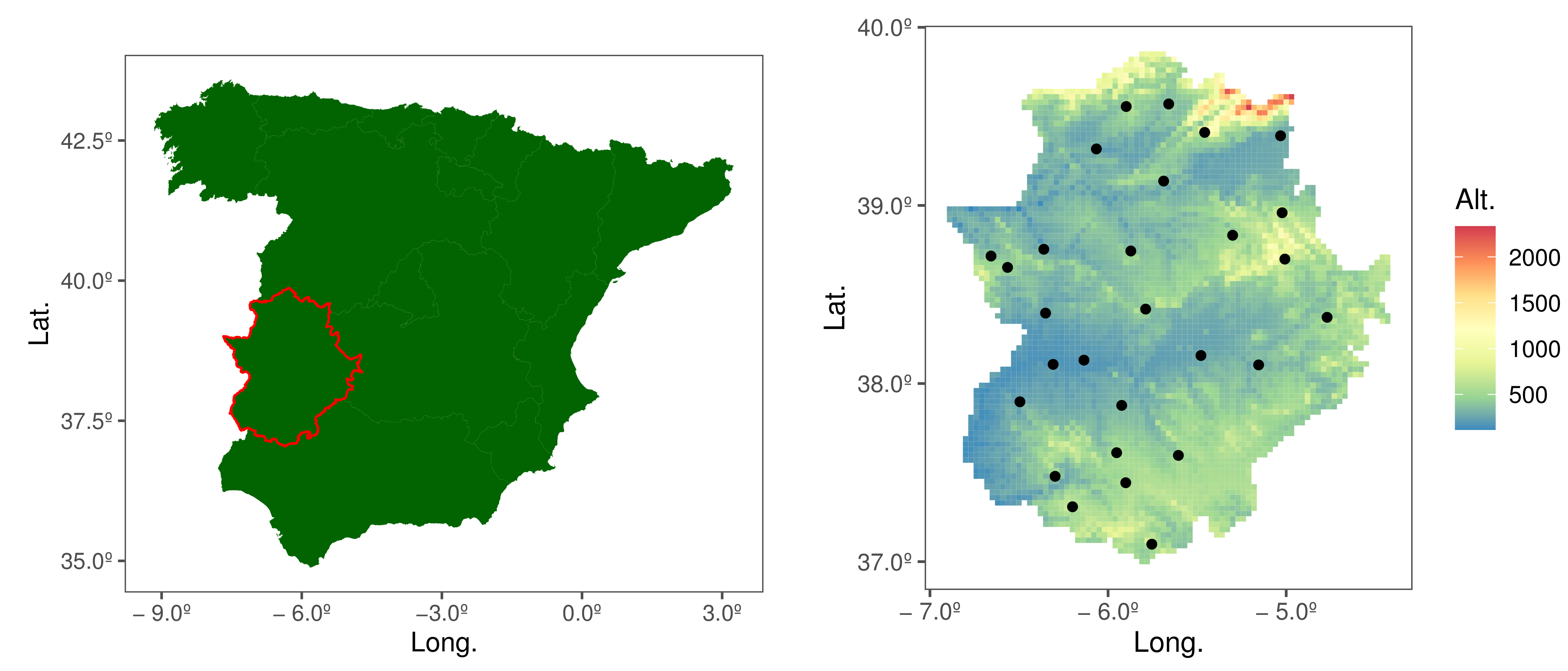
The data used in this study are annual maximum observed temperatures at a set of meteorological observatories distributed over the Extremadura Region (Spain), from 1980 to 2015. These time series were provided by Spain’s State Meteorological Agency (Agencia Estatal de Meteorología, AEMET). Figure 2 shows the location of this region within Spain and the spatial distribution of the observatories considered. In particular, there are $M=28$ meteorological observatories, each providing a time series of $N=36$ extreme temperatures.

For a site $s\in S$, temperature and altitude are correlated, as higher altitudes mean lower temperatures, i.e., temperature decreases with increasing altitude. This reason, together with the fact that Extremadura is not a large region, led us to take the altitude of the sites as being the only covariate in the regression model (5). The altitude was standardized as follows:

$${\tilde{h}}_s={\displaystyle \frac{h_s^{obs}-{min}_s{h}_s}{{max}_s{h}_s-{min}_s{h}_s}},$$

(16)

where $h_s^{obs}$ is the altitude above mean sea level of site $s\in S$, and ${max}_s{h}_s$ and ${min}_s{h}_s$ are the maximum and minimum altitudes of all the sites, respectively.

5. Results

The Bayesian spatial copula model was applied to the described data set (see Section 4). In particular, the BHGCM-200 and BHGCM-210 models were compared using the DIC as a measure of the goodness-of-fit (see Section 3.2). The parameters of the model that best fits the data were compared with the equivalent noncopula model (BHM).

5.1. Evaluation of the Models

As noted above, the DIC was employed to compare the two candidate spatial copula models. The results are presented in

Table 1. Results of using the DIC for the copula models. Boldface indicates the better model.

Model	${\overline{\mathit{D}}}_{\mathit{\theta }}$	$\mathit{D}\left(\overline{\mathit{\theta }}\right)$	${\mathit{p}}_{\mathit{\theta }}$	DIC
BHGCM-200	3697.57	3668.49	29.08	3726.64
BHGCM-210	3589.41	3536.57	52.83	3642.24

. One observes that the copula model in which a spatial model intervenes in the location and scale parameters’ regressions, i.e., BHGCM-210, has a lower DIC value than the model in which the scale parameter is constant (BHGCM-200).

Therefore, the spatial copula model chosen is BHGCM-210.

Table 2. Results of using the DIC for models BHM-210 and BHGCM-210.

Model	${\overline{\mathit{D}}}_{\mathit{\theta }}$	$\mathit{D}\left(\overline{\mathit{\theta }}\right)$	${\mathit{p}}_{\mathit{\theta }}$	DIC
BHM-210	4046.96	3997.51	49.46	4096.42
BHGCM-210	3589.41	3536.57	52.83	3642.24

gives the results of applying the goodness-of-fit to the BHM-210 model. Recall that the parameter $p_{\theta }$ indicates the complexity of the model, and, as can be observed in Table 2, it is greater in the BHGCM model, which was to be expected given that the proposed models are intrinsically more complex. However, this increase in complexity over the models proposed by García et al. [18] is acceptable since the variance in the models proposed in the present work is less than in the BHM cases.

5.2. Parameter Estimates

In this subsection, the regression parameters of the BHM-210 model and the proposed BHGCM-210 model are compared.

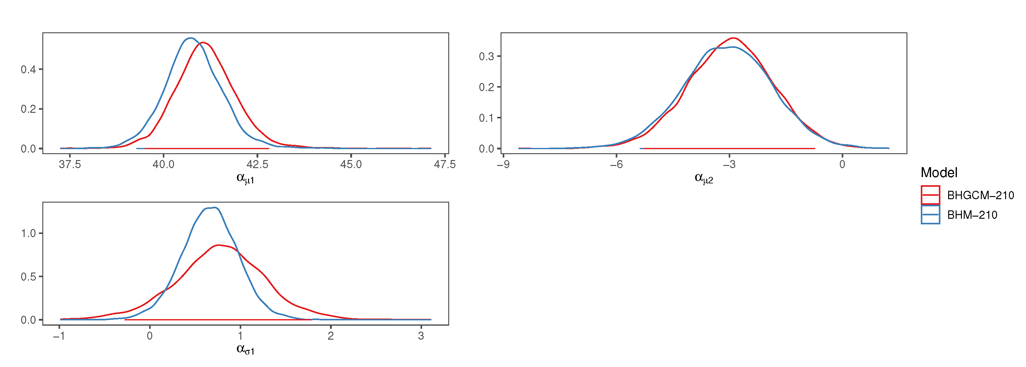
Figure 3 shows the estimate of the posterior distribution density function from the selected BHGCM-210 model (red line) versus that estimated by the BHM-210 model (blue line) for the different regression coefficients $\mathit{\alpha }$. The regression coefficient ${\alpha }_{\sigma 1}$ (lower left panel) of the scale parameter, $\sigma$, has a mean value of 0.78 °C (SD: 0.51 °C) for the BHGCM model. Moreover, this model provides an estimate of the density function that is less concentrated than that given by the BHM model.

With regard to the regression coefficients for the location parameter, $\mu$ (top row), the two models give qualitatively similar posterior density function estimates. In particular, the coefficient ${\alpha }_{\mu 1}$ (top left panel) has a mean of 41.12 °C (SD: 0.84 °C), while the coefficient ${\alpha }_{\mu 2}$ (top right panel) is clearly negative with a mean of −2.97 °C km${}^{-1}$ (SD: 1.15 °C km${}^{-1}$). These negative values are consistent with the fact that temperature decreases with altitude.

Another interesting result is the covariance function of the GEV parameters given by Equation (8).

Table 3. Median (2.5%, 97.5%) of the sill and range coefficients for the location and scale parameters of models BHM-210 and BHGCM-210.

Model	Location Sill	Location Range	Scale Sill	Scale Range
BHM-210	0.52 (0.18, 2.08)	395.07 (132.90, 885.62)	0.25 (0.11, 0.62)	554.84 (235.55, 1110.02)
BHGCM-210	0.53 (0.18, 2.15)	389.82 (125.59, 872.49)	0.27 (0.12, 0.71)	562.47 (233.41, 1133.02)

lists the medians and (2.5%, 97.5%) quantiles of the sill $\left({\beta }_{k0}\right)$ and range $\left({\beta }_{k1}\right)$ coefficients for the location and scale parameters in models BHM-210 and BHGCM-210. The values of these coefficients are of similar orders of magnitude for the two models. Since the range is a measure of the strength of spatial dependence for the location and scale parameters, one observes that, in both models, this dependence is weaker for the location parameter than for the scale parameter.

5.3. Validation of the Models

The posterior predictive distribution (PPD) provides temperature values for the measured observatories that can be compared to the observed temperatures. The error (E) and the absolute error (AE) were used to validate the BHGCM-210 model. These errors were calculated using the values obtained from the PPD. They define as

$$\begin{array}{c}{E}_{st}={\widehat{Y}}_{st}-Y_{st}\hfill \\ \hfill & A{E}_{st}=\left|{\widehat{Y}}_{st}-Y_{st}\right|\hfill \end{array}$$

(17)

where ${\widehat{Y}}_{st}$ is the predictive temperature, $Y_{st}$ is the observed temperature, $s\in S=\{s_1,\dots ,s_M\}$, and $t\in T=\{t_1,\dots ,t_N\}$.

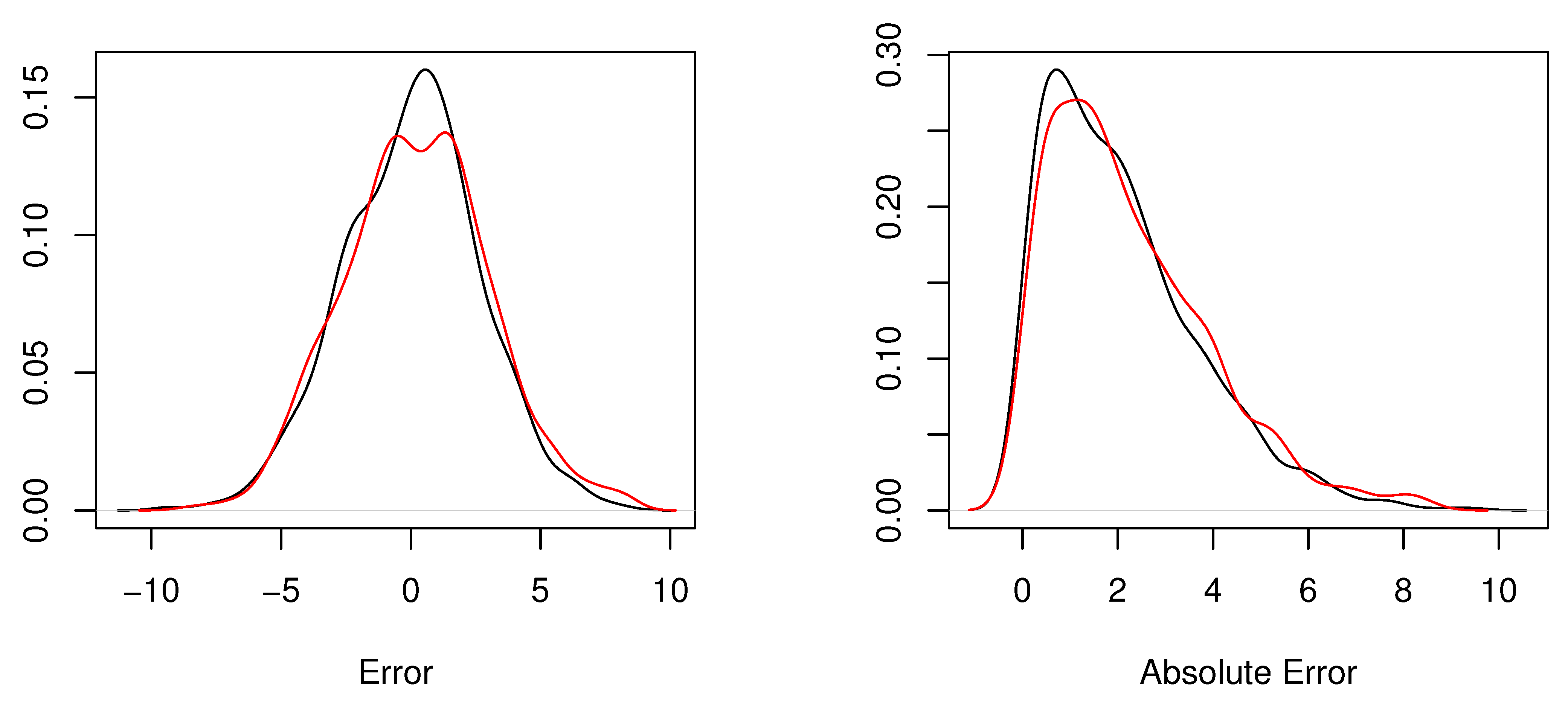
Figure 4 shows the density function of E (left panel) and AE (right panel) for the BHM-210 model (black color) and BHGCM-210 model (red color). The error’s density functions are symmetric around their mean values of 0.23 and 0.06 for the BHGCM-210 and BHM-210 models, respectively. Note that the mean values represent the bias of the models. The precision, measured as the absolute error, is slightly better in the copula model than in the noncopula model. This is related with the increase in uncertainty, previously mentioned in the Introduction.

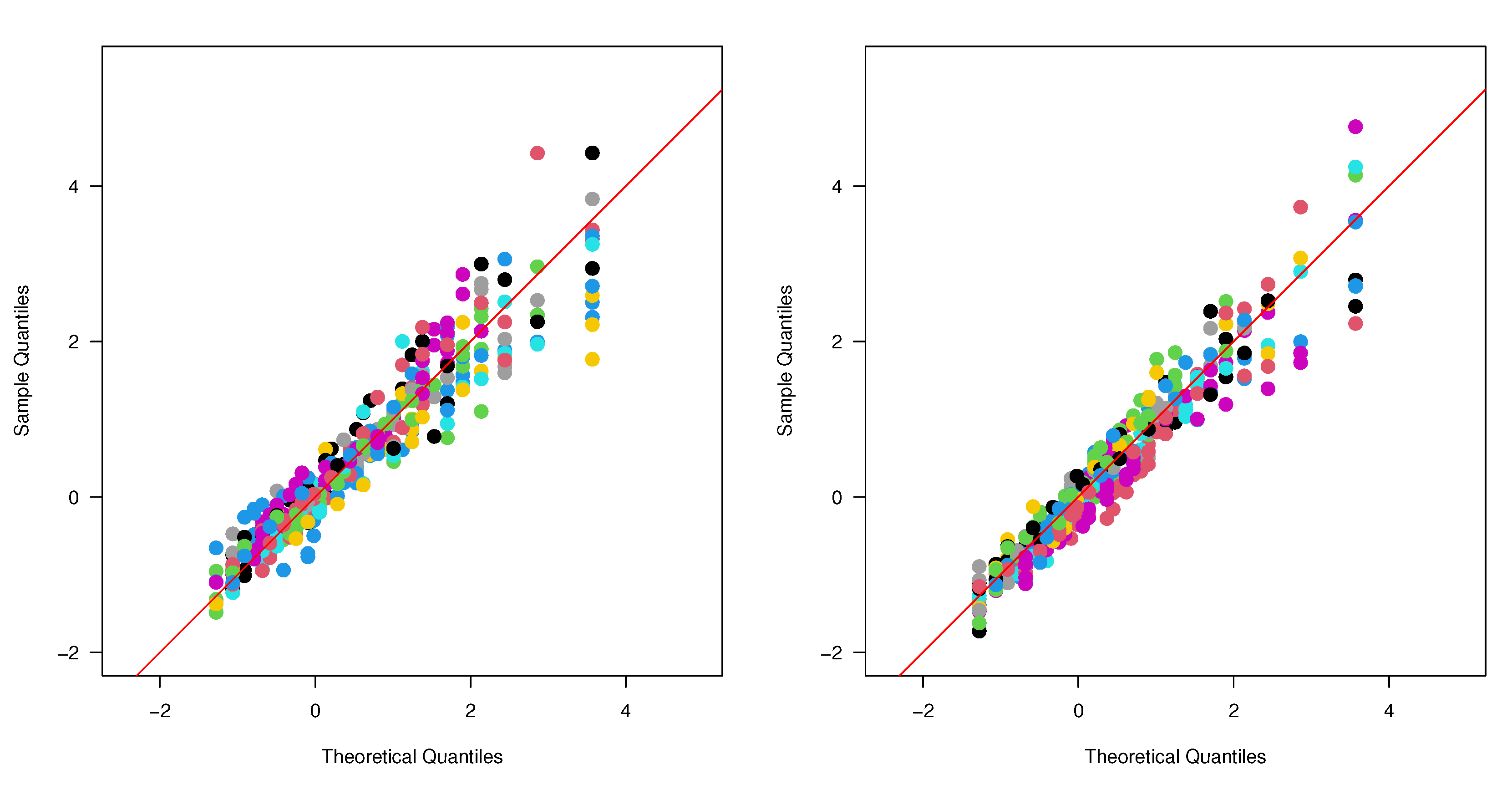
Figure 5 shows the Q-Q plots for all observatories between the theoretical and empirical quantile of $Y_{st}$ and ${\widehat{Y}}_{st}$, respectively, for BHM-210 (left panel) and BHGCM-210 (right panel) models. It can be seen that the ratio between both is close to the red 1:1 line.

5.4. Inference

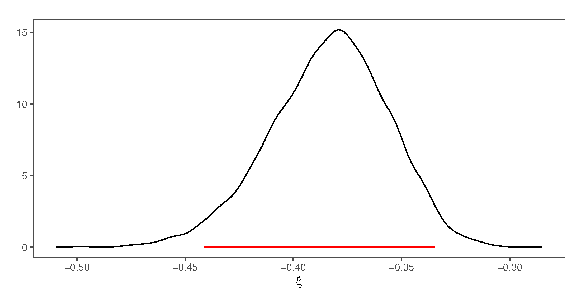
The chosen model (BHGCM-210) estimates the location, scale, and shape parameters of the at-site GEV distribution. These parameters are predicted at the ungauged sites with Algorithm 1. Figure 6 shows the estimated posterior distribution density function for the shape parameter. This parameter takes clearly negative values, with a symmetric and homogeneous distribution around the mean value −0.38 and a standard deviation of 0.03, indicating that there is an upper bound on how high extreme temperatures can be. This leads to a quick decrease of the rate of decay of the extreme temperature distribution, so it does not increase infinitely. Moreover, it is relevant to highlight the low value of the standard deviation obtained when compared with that obtained for the shape parameter estimated in each location individually. Using the maximum-likelihood fit, the standard deviation of the shape parameter varies from 0.09 to 0.12—meaning more than three times that obtained with the spatial model. Therefore, pooling nearby data leads to a decrease in the statistical uncertainty of the parameters and implies an important advantage of using spatial models.

Figure 7 shows the spatial posterior distributions of the means and standard deviations of the location and scale parameters. The spatial posterior distribution of the location parameter shows its dependence on altitude, with mean values between 39.29 °C and 41.12 °C and standard deviations between 1.31 °C and 1.41 °C. The areas with low values of the location parameter correspond to those of higher altitude, since the temperature is highly determined by the orography (see Figure 2). The spatial posterior distribution of the scale parameter shows no spatial dependence, taking very similar values over the entire region (between 2.96 °C and 3.24 °C), and the standard deviations are very concentrated throughout the region.

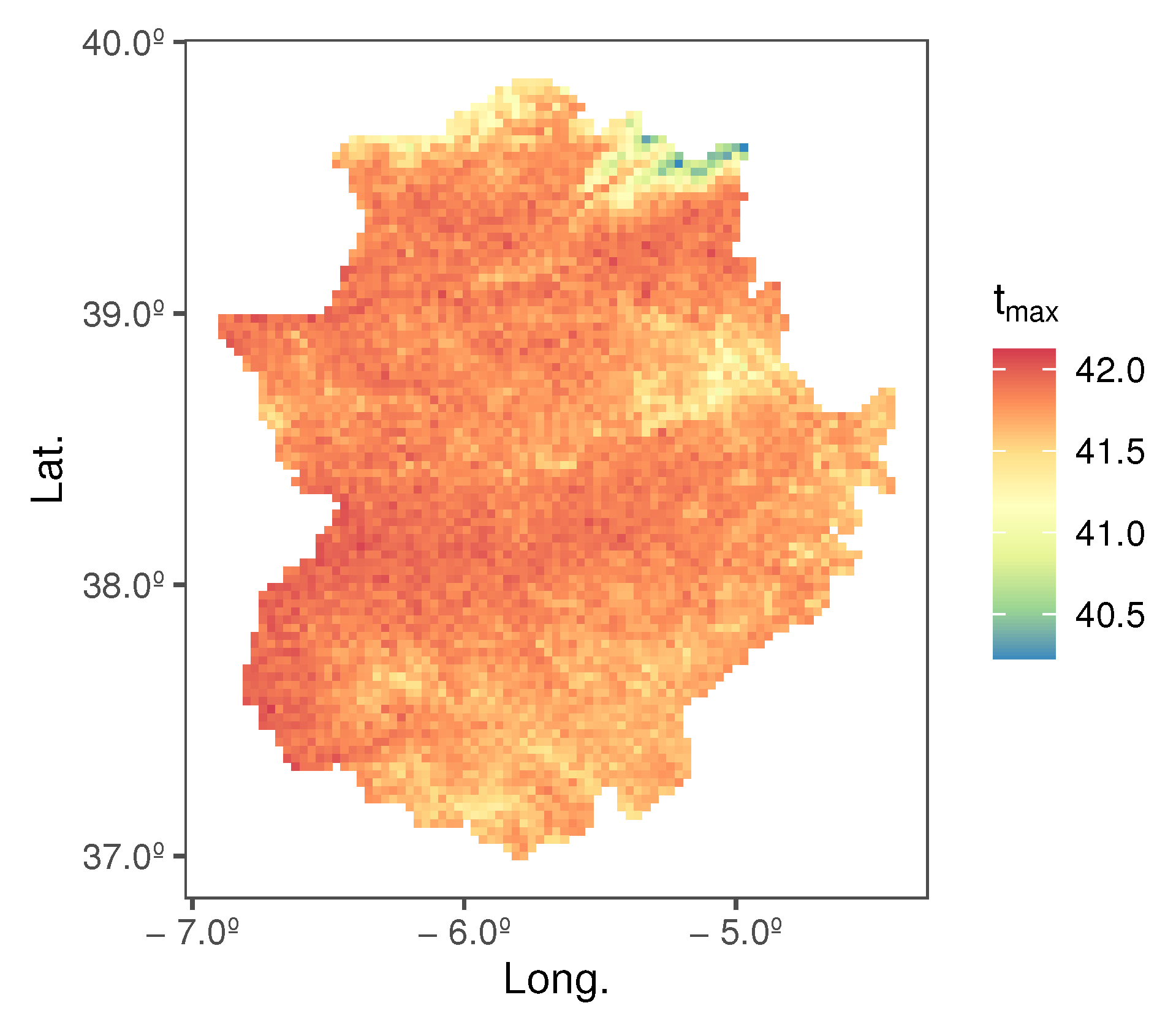
Figure 8 shows the estimation of the maximum temperatures in Extremadura through the posterior predictive distribution. These estimations are consistent with the estimated values for the location parameter given in the previous figure.

6. Conclusions

• Bayesian hierarchical models, BHM, proposed by García et al. [18] present the problem of assuming spatial independence between observations at different sites. The present work has addressed this problem by introducing a copula.
• A Gaussian copula is assumed as a joint distribution with at-site GEV marginal distributions. In this way, the spatial dependence of observations from different sites is represented by a correlation matrix. In addition, spatial regression models of the GEV parameters are proposed.
• Two BHGCM models are proposed: BHGCM-200 takes a spatial regression model for $\mu$ while the parameters $\sigma$ and $\xi$ are constant; BHGCM-210 takes spatial models for $\mu$ and $\sigma$, while the parameter $\xi$ is constant.
• The BHGCM-210 model has a better DIC goodness-of-fit value than the BHGCM-200 model and the noncopula BHM-210 model.
• For the GEV distribution’s location parameter, the BHGCM-210 and BHM-210 models give qualitatively similar estimates of the regression parameter posterior distributions.
• For the GEV distribution’s scale parameter, the BHGCM-210 model gives a distribution with greater variance than that given by the BHM-210 model.
• In the BHGCM-210 model, the GEV shape parameter takes negative values, and its posterior distribution is symmetrical and highly concentrated around −0.38. Therefore, the extreme temperature distribution is not expected to increase too much.
• The BHGCM-210 model gives a spatial posterior distribution for the location parameter that is strongly dependent on altitude, unlike the scale parameter. The location parameter’s mean values in the region lie between 39.29 °C and 41.12 °C.
• In the BHGCM-210 model, the scale parameter’s spatial posterior distribution is very concentrated, taking very similar values throughout the region.

References

1. García, J.; Gallego, M.C.; Serrano, A.; Vaquero, J. Trends in Block-Seasonal Extreme Rainfall over the Iberian Peninsula in the Second Half of the Twentieth Century. J. Clim. 2007, 20, 113–130. [Google Scholar] [CrossRef]
2. Re, M.; Barros, V.R. Extreme rainfalls in SE South America. Clim. Chang. 2009, 96, 119–136. [Google Scholar] [CrossRef]
3. Acero, F.J.; García, J.A.; Gallego, M.C. Peaks-over-Threshold Study of Trends in Extreme Rainfall over the Iberian Peninsula. J. Clim. 2011, 24, 1089–1105. [Google Scholar] [CrossRef]
4. Acero, F.J.; Parey, S.; Hoang, T.T.H.; Dacunha-Castelle, D.; García, J.A.; Gallego, M.C. Non-stationary future return levels for exteme rainfall over Extremadura (SW Iberian Peninsula). Hydrol. Sci. J. 2017, 62, 1394–1411. [Google Scholar] [CrossRef] [Green Version]
5. Wi, S.; Valdés, J.B.; Steinschneider, S.; Kim, T.W. Non-stationary frequency analysis of extreme precipitation in South Korea using peaks-over-threshold and annual maxima. Stoch. Environ. Res. Risk Assess. 2016, 30, 583–606. [Google Scholar] [CrossRef]
6. Nogaj, M.; Yiou, P.; Parey, S.; Malek, F.; Naveau, P. Amplitude and frequency of temperature extremes over the North Atlantic region. Geophys. Res. Lett. 2006, 33. [Google Scholar] [CrossRef]
7. Coelho, C.A.S.; Ferro, C.A.T.; Stephenson, D.B.; Steinskog, D.J. Methods for Exploring Spatial and Temporal Variability of Extreme Events in Climate Data. J. Clim. 2008, 21, 2072–2092. [Google Scholar] [CrossRef] [Green Version]
8. Acero, F.J.; Fernández-Fernández, M.I.; Carrasco, V.M.S.; Parey, S.; Hoang, T.T.H.; Dacunha-Castelle, D.; García, J.A. Changes in heat wave characteristics over Extremadura (SW Spain). Theor. Appl. Climatol. 2018, 133, 605–617. [Google Scholar] [CrossRef] [Green Version]
9. Ramos, A.A. Extreme value theory and the solar cycle. Astron. Astrophys. 2007, 472, 293–298. [Google Scholar] [CrossRef] [Green Version]
10. Acero, F.J.; Carrasco, V.M.S.; Gallego, M.C.; García, J.A.; Vaquero, J.M. Extreme Value Theory Applied to the Millennial Sunspot Number Series. Astrophys. J. 2018, 853, 80. [Google Scholar] [CrossRef] [Green Version]
11. Longin, F.M. From value at risk to stress testing: The extreme value approach. J. Bank. Financ. 2000, 24, 1097–1130. [Google Scholar] [CrossRef]
12. Castillo, E.; Hadi, A.S.; Balakrishnan, N.; Sarabia, J.M. Extreme Value and Related Models with Applications in Engineering and Science; Wiley: Hoboken, NJ, USA, 2004. [Google Scholar]
13. Casson, E.; Coles, S. Spatial regression models for extremes. Extremes 1999, 1, 449–468. [Google Scholar] [CrossRef]
14. Cooley, D.; Nychka, D.; Naveau, P. Bayesian spatial modeling of extreme precipitation return levels. J. Am. Stat. Assoc. 2007, 102, 824–840. [Google Scholar] [CrossRef]
15. Portero, J.; Acero, F.J.; García, J.A. Analysis of Extreme Temperature Events over the Iberian Peninsula during the 21st Century Using Dynamic Climate Projections Chosen Using Max-Stable Processes. Atmosphere 2020, 11, 506. [Google Scholar] [CrossRef]
16. Davison, A.C.; Padoan, S.A.; Ribatet, M. Statistical modeling of spatial extremes of spatial extremes. Stat. Sci. 2012, 27, 161–186. [Google Scholar] [CrossRef] [Green Version]
17. Acero, F.J.; García, J.A.; Gallego, M.C.; Parey, S.; Dacunha-Castelle, D. Trends in summer extreme temperatures over the Iberian Peninsula using nonurban station data. J. Geophys. Res. Atmos. 2014, 119, 39–53. [Google Scholar] [CrossRef]
18. García, A.; Martín, J.; Naranjo, L.; Acero, F.J. A Bayesian hierarchical spatio-temporal model for extreme rainfall in Extremadura (Spain). Hydrol. Sci. J. 2018, 63, 878–894. [Google Scholar] [CrossRef]
19. Renard, B.; Lang, M. Use of a Gaussian copula for multivariate extreme value analysis: Some case studies in hydrology. Adv. Water Resour. 2007, 30, 897–912. [Google Scholar] [CrossRef] [Green Version]
20. Renard, B. A Bayesian hierarchical approach to regional frequency analysis. Water Resour. Res. 2011, 47, 11513. [Google Scholar] [CrossRef] [Green Version]
21. Liu, Y.R.; Li, Y.P.; Ma, Y.; Jia, Q.M.; Su, Y.Y. Development of a Bayesian-copula-based frequency analysis method for hydrological risk assessment—The Naryn River in Central Asia. J. Hydrol. 2020, 580, 124349. [Google Scholar] [CrossRef]
22. Beck, N.; Genest, C.; Jalbert, J.; Mailhot, M. Predicting extreme surges from sparse data using a copula-based hierarchical Bayesian spatial model. Environmetrics 2020, 31, e2616. [Google Scholar] [CrossRef] [Green Version]
23. Salvadori, G.; De Michele, C.; Kottegoda, N.T.M.; Rosso, R. Extremes in Nature: An Approach Using Copulas; Springer Science & Business Media: Berlin/Heidelberg, Germany, 2007; Volume 56. [Google Scholar]
24. Sklar, A. Fonctions de répartition à n dimensions et leurs marges. Publ. Inst. Statist. Univ. Paris 1959, 8, 229–231. [Google Scholar]
25. Genest, C.; Favre, A.C.; Béliveau, J.; Jacques, C. Metaelliptical copulas and their use in frequency analysis of multivariate hydrological data. Water Resour Res. 2007, 43, W09401. [Google Scholar] [CrossRef] [Green Version]
26. Favre, A.C.; El Adlouni, S.; Perreault, L.; Thiémonge, N.; Bobée, B. Multivariate hydrological frequency analysis using copulas. Water Resour. Res. 2004, 40. [Google Scholar] [CrossRef] [Green Version]
27. Wikle, C.K.; Berliner, M.L.; Cressie, N. Hierarchical Bayesian space-time models. Environ. Ecol. Stat. 1998, 5, 117–154. [Google Scholar] [CrossRef]
28. Sun, X.; Thyer, M.; Renard, B.; Lang, M. A general regional frequency analysis framework for quantifying local-scale climate effects: A case study of ENSO effects on Southeast Queensland rainfall. J. Hydrol. 2014, 512, 53–68. [Google Scholar] [CrossRef] [Green Version]
29. Dyrrdal, A.V.; Lenkoski, A.; Thorarinsdottir, T.L.; Stordal, F. Bayesian hierarchical modeling of extreme hourly precipitation in Norway. Environmetrics 2015, 26, 89–186. [Google Scholar] [CrossRef] [Green Version]
30. Ragulina, G.; Reitan, T. Generalized extreme value shape parameter and its nature for extreme precipitation using long time series and Bayesian approach. Hydrol. Sci. J. 2017, 62, 863–879. [Google Scholar] [CrossRef]
31. Barlow, A.M.; Rohrbeck, C.; Sharkey, P.; Shooter, R.; Simpson, E.S. A Bayesian spatio-temporal model for precipitation extremes-STOR team contribution to the EVA2017 challenge. Extremes 2018, 21, 431–439. [Google Scholar] [CrossRef] [Green Version]
32. Craigmile, P.F.; Guttorp, P. Can a regional climate model reproduce observed extreme temperatures? Statistica 2013, 73, 103–122. [Google Scholar]
33. Daraio, J.A.; Amponsah, A.O.; Sears, K.W. Bayesian Hierarchical Regression to Assess Variation of Stream Temperature with Atmospheric Temperature in a Small Watershed. Hydrology 2017, 4, 44. [Google Scholar] [CrossRef] [Green Version]
34. Gnedenko, B. Sur la distribution limite du terme maximum d’une serie aleatorie. Ann. Math. 1943, 44, 423–453. [Google Scholar] [CrossRef]
35. Fisher, R.A.; Tippett, L.H.C. Limiting forms of the frequency distribution of the largest or smallest member of a sample. In Mathematical Proceedings of the Cambridge Philosophical Society; Cambridge University Press: Cambridge, UK, 1928; Volume 24, pp. 180–190. [Google Scholar]
36. Coles, S. An Introduction to Statistical Modeling of Extreme Values; Springer: London, UK, 2001; Volume 208. [Google Scholar]
37. Gilks, W.R.; Richardson, S.; Spiegelhalter, D.J. Introducing Markov Chain Monte Carlo. In Markov Chain Monte Carlo in Practice; Chapman & Hall: New York, NY, USA, 1996. [Google Scholar]
38. Cowles, M.K.; Carlin, B.P. Markov chain Monte Carlo convergence diagnostics: A comparative review. J. Am. Stat. Assoc. 1996, 91, 883–904. [Google Scholar] [CrossRef]
39. Martyn, P.; Nicky, B.; Kate, C.; Karen, V. CODA: Convergence diagnosis and output analysis for MCMC. R News 2006, 6, 7–11. [Google Scholar]
40. Wickham, H. ggplot2. Elegant Graphics for Data Analysis; Version, 2 (1); Springer-Verlag: New York, NY, USA, 2016. [Google Scholar]
41. Centro Nacional de Información Geográfica. Modelo Digital del Terreno 2015 CC-BY 4.0. Available online: http://www.scne.es/ (accessed on 9 July 2021).
42. Spiegelhalter, D.J.; Best, N.G.; Carlin, B.P.; van der Linde, A. The deviance information criterion: 12 years on. J. R. Stat. Soc. 2014, 76, 485–493. [Google Scholar] [CrossRef]
43. Gelman, A.; Carlin, J.; Stern, H.; Rubin, D. Bayesian Data Analysis, 2nd ed.; Texts in Statistical Science; Chapman and Hall: New York, NY, USA, 1995; 696p. [Google Scholar]
Figure 1. Stages of the Bayesian hierarchical model.
Atmosphere 12 00897 g001
Figure 2. Location of the Extremadura Region within Spain (left). Topographic map of Extremadura together with the locations of the meteorological observatories used in this study (right).
Atmosphere 12 00897 g002
Figure 3. Estimated posterior distribution density functions of the regression coefficients α k 1 (left) and α k 2 (right) for the location (top row) and scale (bottom row) parameters for the models BHM-210 (blue line) and BHGCM-210 (red line). The red horizontal lines show the 0.025 to 0.975 quantiles.
Atmosphere 12 00897 g003
Figure 4. Validation of the BHM-210 (black color) and BHGCM-210 (red color) models for all the observatories: E (left) and AE (right) density functions.
Atmosphere 12 00897 g004
Figure 5. Validation of the BHM-210 (left) and BHGCM-210 (right) models for all the observatories: Q-Q plots.
Atmosphere 12 00897 g005
Figure 6. Estimated posterior distribution density function for the shape parameter. The red horizontal line shows the 0.025 to 0.975 quantile.
Atmosphere 12 00897 g006
Figure 7. Spatial posterior distributions of the mean (left) and the standard deviation (right) of the location (top row) and scale (bottom row) parameters.
Atmosphere 12 00897 g007
Figure 8. Spatial posterior predictive distribution of the maxima temperature.
Atmosphere 12 00897 g008