Atmospheric PM2.5 Prediction Using DeepAR Optimized by Sparrow Search Algorithm with Opposition-Based and Fitness-Based Learning

Abstract

There is an important significance for human health in predicting atmospheric concentration precisely. However, due to the complexity and influence of contingency, atmospheric concentration prediction is a challenging topic. In this paper, we propose a novel hybrid learning method to make point and interval predictions of PM2.5 concentration simultaneously. Firstly, we optimize Sparrow Search Algorithm (SSA) by opposition-based learning, fitness-based learning, and Lévy flight. The experiments show that the improved Sparrow Search Algorithm (FOSSA) outperforms SSA-based algorithms. In addition, the improved Sparrow Search Algorithm (FOSSA) is employed to optimize the initial weights of probabilistic forecasting model with autoregressive recurrent network (DeepAR). Then, the FOSSA–DeepAR learning method is utilized to achieve the point prediction and interval prediction of PM2.5 concentration in Beijing, China. The performance of FOSSA–DeepAR is compared with other hybrid models and a single DeepAR model. Furthermore, hourly data of PM2.5 and O₃ concentration in Taian of China, O₃ concentration in Beijing, China are used to verify the effectiveness and robustness of the proposed FOSSA–DeepAR learning method. Finally, the empirical results illustrate that the proposed FOSSA–DeepAR learning model can achieve more efficient and accurate predictions in both interval and point prediction.

1. Introduction

As one of the pollutants under public concern, PM2.5 concentration has a vital impact on air quality and human health. High concentration of PM2.5 will result in poor air quality and cause harm to human health, such as respiratory diseases, and even death in severe cases. Furthermore, the fluctuation of PM2.5 concentration has negative impacts on the travelling and working of residents. Thus, accurate prediction of PM2.5 concentration is significant for alerting residents before the high concentrations of PM2.5 occur. It is helpful for residents to arrange their outdoor activities flexibly, and reduce the health damage caused by bad air quality.

Over the past few years, most models established for PM2.5 concentration prediction are based on the time series analysis method [1]. However, the nonstationarity of atmospheric concentration brings a great challenge for accurate prediction. In recent years, some methods are proposed to predict atmospheric concentration such as the distribution-based method, machine learning, and optimization algorithms. For instance, Cavieres et al. [2] proposed a method based on bivariate control charts with heavy-tailed asymmetric distributions to monitor environmental quality. Puentes et al. [3] used bivariate regression and Birnbaum–Saunders distributions to predict PM2.5 and PM10 concentration. Jiang et al. [4] proposed a hybrid approach based on extreme learning machine (ELM) optimized by pigeon-inspired optimization (PIO) to predict the price. Wong et al. [5] applied a land use regression and extreme gradient boosting to predict PM2.5 concentration. Lu et al. [6] proposed a learning approach which combined long short-term memory (LSTM) and 3D numerical model with 3D-VAR. Jiang et al. [7] proposed a hybrid model based on the group teaching optimization algorithm (GTOA) and ELM. Huang et al. [8] used empirical mode decomposition (EMD) to decompose the time series of PM2.5 concentration, and then applied gated recurrent units (GRU) to forecast single sub-sequence. Jiang et al. [9] established a hybrid model which composed of the improved pigeon-inspired optimization (IPIO) algorithm and ELM. Recently, sparrow search algorithm (SSA) [10] was proposed, which outperformed particle swarm optimization (PSO) [11], grey wolf optimizer (GWO) [12] and gravitational search algorithm (GSA) [13]. In addition, some improved SSA algorithms have been proposed to enhance the search ability. For example, Yuan et al. [14] proposed an improved sparrow search algorithm (ISSA) by using the centroid opposition-based learning (COBL) method. Liu et al. [15] proposed a modified sparrow search algorithm (CASSA) optimized by chaotic strategy, adaptive inertia weight and Cauchy–Gaussian mutation strategy. Li [16] proposed a hybrid sparrow search algorithm (HSSA) with opposition-based learning to improve quality of initial population. Zhang et al. [17] proposed a chaotic sparrow search algorithm (CSSA) using logistic mapping, adaptive inertia weight, and a self-adaptive updating formula. Lévy flight (LF) mechanism and chaos mechanism were utilized in a balanced sparrow search algorithm (BSSA) proposed in [18]. The position updating method in the bird swarm algorithm (BSA) was applied to improve SSA [19]. In this paper, we use opposition-based learning, Lévy flight, and fitness-based learning to improve SSA.

However, most of the previous research focused on the point prediction of atmospheric concentration, which is insufficient to guarantee the reliability of air quality forecast. As we know, interval prediction is helpful for quantifying uncertainty caused by accidental factors. It can provide the upper and lower bounds of atmospheric concentration and more valuable information. Salinas et al. [20] proposed the autoregressive recurrent networks (DeepAR) model to achieve point and interval prediction of the time series. The output of DeepAR is not a simple forecast value, but the probability distribution. At present, DeepAR model has been utilized to forecast sales volume, traffic occupancy rate, electricity, and deformation prediction [21]. To the best of our knowledge, DeepAR is not used to predict atmospheric concentration. In this paper, DeepAR model is utilized in the field of air quality prediction in order to simultaneously achieve the point and interval prediction of PM2.5 and O₃ concentration. In addition, as a novel swarm intelligence optimization algorithm, we will improve SSA by using opposition-based learning, Lévy flight, and fitness-based learning (FOSSA). Here, the opposition-based learning method is used to initialize population to improve diversity and quality of initial population. Lévy flight is used in the updating methods of producers and alarmers. This is helpful for avoiding local optimal solution, while fitness-based learning is utilized to endow the population with powerful global search capability. Moreover, the proposed FOSSA is used to optimize the initial weights of DeepAR. Finally, the point prediction and interval prediction of PM2.5 concentration are given by using the FOSSA–DeepAR learning model. Additionally, the proposed FOSSA–DeepAR model has good robustness in prediction of O₃ concentration.

The remaining sections of this paper is organized as follows. Section 2 introduces some methodologies utilized in this paper and then gives an improved SSA with opposition-based learning, Lévy flight, and fitness-based learning. At the same time, we employ some benchmark functions to show the effectiveness of FOSSA. Section 3 shows the experimental results and analysis of prediction result of FOSSA–DeepAR model. Finally, conclusions and further research are given.

2. Methods

2.1. Sparrow Search Algorithm

SSA [10] is a novel swarm optimization approach inspired by the search behavior of sparrow population. The sparrow population consists of producers and scroungers, and the two kinds of sparrows follow different rules to update their positions. In order to find food, sparrows flexibly transform their roles between the producers and scroungers and then perform different search behaviors. Some sparrows will send out warning messages and immediately move to the safe area when they detect the predators. The sparrows who detect the danger are called alarmers in this paper.

There are two ways for producers to update their positions. The one way is executed when the producer does not receive the warning signal issued by the alarmer. In this case, the updated location of producers is shown in Equation (1).

$$P_{i,j}^{t+1}=P_{i,j}^t\times \exp \left(\frac{-i}{\alpha \times \mathrm{epoch}}\right), R_2<ST,$$

(1)

where t indicates the current iteration. Epoch denotes the maximum number of iterations and $\alpha$ is a random number between 0 and 1. $P_{i,j}$ represents the value of the j-th dimension of the i-th individual and d is the dimension of the problem we want to solve. ST ($ST\in \left[0.5, 1\right]$) and $R_2$ ($R_2\in \left[0, 1\right]$) represent the threshold value and the warning value, respectively.

The other way is implemented when the warning signal is received by the producer. The producer knows that the predator is approaching, and then guides all sparrows to a safe area. The location is updated as Equation (2).

$$P_{i,j}^{t+1}=P_{i,j}^t+r\times D, R_2\ge ST,$$

(2)

where r is a random number that obeys the normal distribution, and D is a $1\times d$ matrix in which all elements are 1.

Some scroungers with better fitness will move towards the best producer, whose positions are updated as Equation (3).

$$P_{i,j}^{t+1}=P_{\mathrm{best}}^{t+1}+\left|P_{i,j}^t-P_{\mathrm{best}}^{t+1}\right|\times A^{+}\times D, i\le \frac{n}{2},$$

(3)

where $P_{best}$ represents the optimal position of the entire population. A is a $1\times d$ matrix, in which all elements are 1 or −1. $A^{+}=A^T{\left(A{A}^T\right)}^{-1}$.

The remaining scroungers with poor fitness will continue to search for food near the previous location. This kind of scrounger updates their position as Equation (4).

$$P_{i,j}^{t+1}=r\times \exp \left(\frac{P_{\mathrm{worst}}^t-P_{i,j}^t}{i^2}\right), i>\frac{n}{2}.$$

(4)

If the producer of optimal position perceives danger, it will become an alarmer and the entire group must be led to a safe area. In this situation, the location of the alarmer is updated as Equation (5).

$$P_{i,j}^{t+1}=P_{i,j}^t+K\times \left(\frac{\left|P_{i,j}^t-P_{\mathrm{worst}}^t\right|}{\left(f_i-f_{\mathrm{w}}\right)+\epsilon }\right), f_i=f_g,$$

(5)

where K is a random number between −1 and 1, and $f_i$, $f_g$, and $f_w$ represent the current fitness value of the sparrow, the current optimal fitness value and the worst fitness value of the entire group, respectively. Let $\epsilon \ge 0$ is a small constant in order to ensure that the denominator is not 0.

If the alarmer is not located in the best position, the alarmer will move towards the optimal position in order to reduce the probability of being preyed. The location updated as Equation (6).

$$P_{i,j}^{t+1}=P_{\mathrm{best}}^t+\beta \times |P_{i,j}^t-P_{\mathrm{best}}^t|, f_i>f_g$$

(6)

2.2. Sparrow Search Algorithm with Fitness-Based and Opposition-Based Learning

In this paper, the opposition-based learning, Lévy flight, and fitness-based learning are used to improve the performance of SSA. The improvement of FOSSA mainly comes from three aspects. First of all, we use opposition-based learning to increase the diversity and quality of the initial population. Secondly, the Lévy flight is utilized to update the positions of producers and alarmers. Finally, the fitness-based learning method is employed to enhance the search ability of the sparrow population. The improvement details of FOSSA are summarized as follows.

2.2.1. Opposition-Based Learning

In the ordinary SSA [10], the positions of the initial population are randomly initialized. The diversity and quality of the initial population, generated by random initialization method, are not guaranteed. Accordingly, the accuracy of the SSA solution decreases. The opposition-based learning method can greatly improve the quality of the initial population.

The steps of initializing the population via opposition-based learning are described as follows:

Step 1.

Generate N individuals by random initialization, and calculate the center of gravity of N individuals. The calculation method of the center of gravity is expressed as Equation (7):

$$G_j=\frac{{{\displaystyle \sum }}_{j=1}^d{X}_{i,j}}{n},$$

(7)

where $G_j$ represents the center of gravity of the j-th dimension, n is the number of sparrows, and d is the dimension;

Step 2.

alculate the opposite position of each individual. The calculation method is shown as Equation (8);

$${\overline{X}}_i=2\times G-X_i, i=1,2,3,\cdots n.$$

(8)

Step 3.

Make sure the position of the anti-center of gravity individual within the search scope. The method is shown as Equation (9):

$${\overline{X}}_{i,j}=\{\begin{array}{c}{\min }_j+\mathrm{rand}\left(0, 1\right)\times \left(G_j-{\min }_j\right), \mathrm{if} {\overline{X}}_{i,j}<{\min }_j\\ G_j+\mathrm{rand}\left(0, 1\right)\times \left({\max }_j-G_j\right), \mathrm{if} {\overline{X}}_{i,j}>{\max }_j .\end{array}$$

(9)

where ${\min }_j=\min \left(X_{i,j}\right),{\max }_j=\max \left(X_{i,j}\right);$

Step 4.

Calculate the fitness value of 2N individuals, and select N individuals with the best fitness as the initial individuals of the population.

2.2.2. Lévy Flight

In BSSA, the Lévy flight is used to update a single parameter in Equation (6), but sparrows cannot avoid local optimum effectively. Lévy flight is applied in this paper to update the entire position of producers and alarmers. Equations (2) and (6) are changed as Equations (10)–(12).

$$\sigma =\frac{\mathrm{gamma}\left(1+\tau \right)\times \sin \left(\pi \times \tau ÷2\right)}{\mathrm{gamma}\left(\left(1+\tau \right)÷2\right)\times \tau \times 2^{\frac{\tau -1}{2}}},$$

(10)

$$s=\frac{\partial }{{\left|v\right|}^{\frac{1}{\tau }}},$$

(11)

$$P_{i.j}^{t+1}=m\times \mathrm{step}\times s\times \left(P_{i,j}^t-P_{\mathrm{best},j}^t\right)$$

(12)

where gamma represents the gamma function. $\tau$ is a hyperparameter, and this article sets the value of $\tau$ as 1. $\partial$ and v are random variables which obey the normal distribution $N\left(0,{\sigma }^2\right)$ and$N\left(0,1\right)$, respectively. Moreover, m is a random number, and s is the step size whose value is 0.001. $P_{\mathrm{best},j}$ represents the value of the global optimal position in the j-th dimension at the previous iteration.

2.2.3. Fitness-Based Learning

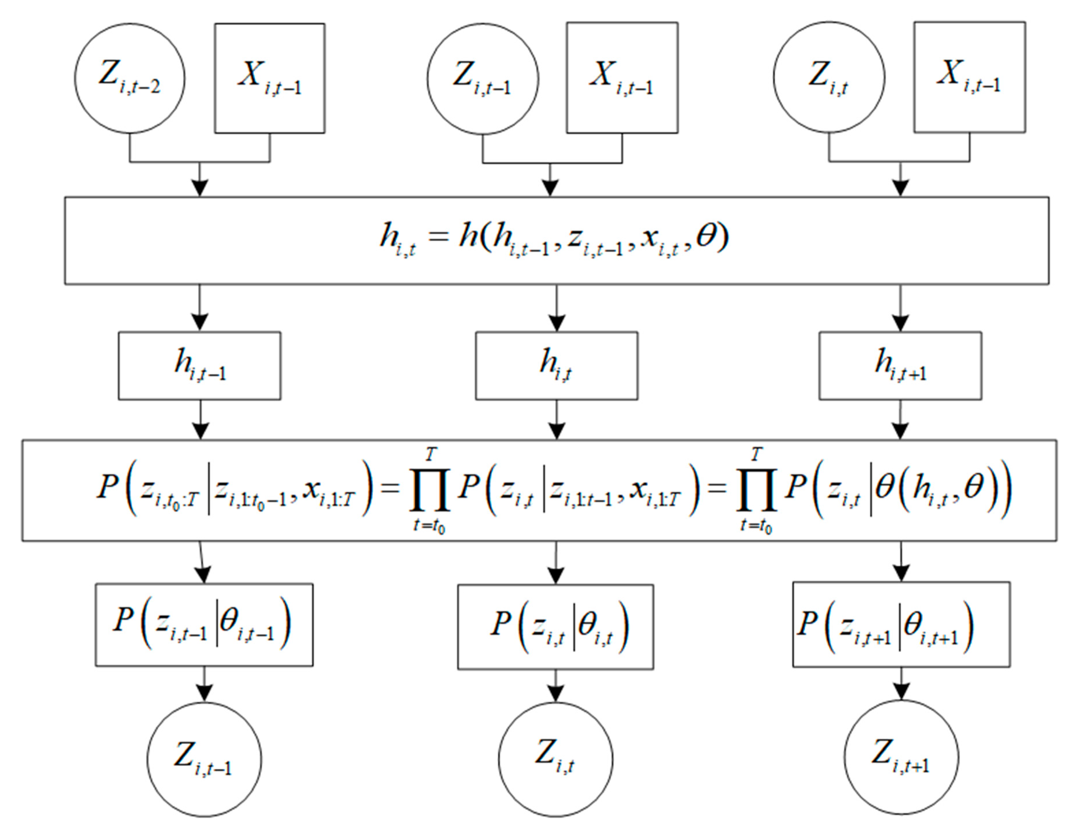
On the one hand, some individuals will fall into the local optimum during the searching process, and their positions will not change during several continuous iterations. The part of sparrows, which can be regarded as lack of search ability, should be updated in the subsequent search process to increase the convergence speed and accuracy.

On the other hand, the producers in SSA are responsible for determining the search direction of the entire population and search in wider space. Accordingly, the producers are vital for whether the population can move towards the optimal result. The scroungers follow the producers and search for food near producers. It follows that the scrounger can improve the accuracy of the solution. In the original SSA, the number of producers and scroungers is fixed. There are too many producers in the early stage of the search process that the population cannot move towards the correct search direction quickly. In the later stage of the search process, the search scope gradually concentrates on a small range. In the later searching process, many scroungers are bad for exploring the high valuable area.

Therefore, this paper utilizes fitness-based learning to endow the population with powerful global search capability. First of all, inspired by the transformation behavior of employed bees to onlooker in an artificial bee colony (ABC) [22], fitness-based learning is introduced into FOSSA. If an individual does not update its position during 5 consecutive iterations, the individual will get a new position generated randomly. In addition, we adjust the number of producers and scroungers based on fitness value during the search process. The fitness value of each individual is calculated as Equation (13):

$$fit\left(X_i\right)=\{\begin{array}{c}\frac{1}{1+f\left(X_i\right)} \mathrm{if} f\left(X_i\right)\ge 0\\ 1+\left|f\left(X_i\right)\right| \mathrm{otherwise}\end{array},$$

(13)

where $f\left(·\right)$ is the objective function for a minimization problem. Individuals with fitness greater than 0.9 will perform the tasks of the producer. When the fitness value of a sparrow is greater than 0.7 but less than 0.9, the sparrow will become a scrounger. It will leave its current position immediately and approach the optimal producer. If the fitness value is less than 0.7, the sparrow becomes a scrounger but will not move towards the best producer. The flowchart of FOSSA is shown in Figure 1.

2.3. DeepAR

Probabilistic forecasting with autoregressive recurrent networks (DeepAR), proposed by Salinas et al., is a novel forecasting method which could achieve accurate probabilistic forecasts. Combining several related time series together, this forecasting method could not only learn a global model from analogous time series, but also provides flexibility to achieve point prediction, interval prediction, or both. In addition, time step of prediction is also a selectable hyperparameter in this method.

The goal of DeepAR is to model the conditional distribution which is presented as Equation (14):

$$P(z_{i,t_0:T}|z_{i,1:t_0-1}, x_{i,1:T}),$$

(14)

where $z_{i,t}$ is the value of time series i at time t. Given the past series $\left[z_{i,1},z_{i,2},\cdots ,z_{i,t_0-2},z_{i,t_0-1}\right]$, this model can be employed to predict the future series $\left[z_{i,t_0},z_{i,t_0+1},\cdots ,z_{i,T}\right]$, where the t₀ is the time point from which $z_{i.t}$ needs to be predicted. $\left[1:t_0-1\right]$ and $\left[t_0:T\right]$ represent the conditioning range and prediction range, respectively. The DeepAR model will predict the value of prediction range based on the value of the conditioning range. If covariate time series $x_i$ is introduced in the model, the value of the $x_i$ from time 1 to time T ($x_{i,1:T}$) will also be used for forecasting. However, the value of covariate time series must be available during the entire time period.

How the model works in conditioning range is shown in Figure 2. DeepAR assumes that $P(z_{i,t_0:T}|z_{i,1:t_0-1},x_{i,1:T})$ consists of likelihood factors. These likelihood factors are defined as Equations (15) and (16).

$$P\left(z_{i,t_0:T}|z_{i,1:t_0-1},x_{i,1:T}\right)={\displaystyle \prod }_{t=t_0}^{T}P\left(z_{i,t}|z_{i,1:t-1},x_{i,1:T}\right)={\displaystyle \prod }_{t=t_0}^{T}P(z_{i,t}|\theta \left(h_{i,t},\mathsf{\theta }\right)),$$

(15)

$$h_{i,t}=h\left(h_{i,t-1},z_{i,t-1},x_{i,t},\mathsf{\theta }\right) ,$$

(16)

where $h_{i,t}$ is the output of a multi-layer recurrent neural network constructed by an LSTM cell which is parametrized by Ɵ. Given a time series as conditioning range, we can obtain $h_{i,t_o-1}$ by Equation (16) as the initial state. For prediction range, we can sample ${\tilde{z}}_{i,t}$ by $P(·|\theta \left({\tilde{h}}_{i,t-1},\mathsf{\theta }\right))$, where ${\tilde{h}}_{i,t}=h\left(h_{i,t-1},{\tilde{z}}_{i,t},x_{i,t-1},\mathsf{\theta }\right)$. The samples achieved in this way could be used to compute some statistics we are interested in, such as the mean and quantile, in a future period.

In this paper, we assume PM2.5 concentration obeys normal distribution. We give z by Equation (17). Here, $\mu$ and $\sigma$ are given by Equations (18) and (19). After training the model by using the conditioning range, the trained model is used to predict the mean value $\mu$ and variance $\sigma$ of each time point. Then, we can obtain joint samples by using $N\left(\mu ,\sigma \right)$ and use them to compute some statistics of interest.

$$P(z|\mu ,\sigma )={\left(2\mathsf{\pi }{\sigma }^2\right)}^{-\frac{1}{2}}\exp \left(-{\left(z-\mu \right)}^2/\left(2{\sigma }^2\right)\right),$$

(17)

$$\mu \left(h_{i,t}\right)=w_{\mu }^T{h}_{i,t}+b_{\mu } ,$$

(18)

$$\sigma \left(h_{i,t}\right)=\log \left(1+\exp \left(w_{\sigma }^T{h}_{i,t}+b_{\sigma }\right)\right) .$$

(19)

2.4. Framework of FOSSA–DeepAR

In order to provide an accurate point prediction and interval prediction of PM2.5 concentration, a novel hybrid model is established based on the FOSSA and DeepAR. FOSSA is utilized to optimize the initial weights of DeepAR. The structure of the proposed approach is summarized as follows:

Step 1.

Data preprocessing. In order to avoid the gradient vanishing and gradient exploding problem, the data is standardized before training model;

Step 2.

Establish DeepAR model. In this study, the recurrent neural network used in DeepAR is the long short-term memory (LSTM) model. In addition, we assume that PM2.5 concentration follows a Gaussian distribution;

Step 3.

Optimize the initial weights of DeepAR via FOSSA. It is inefficient and unnecessary to use all samples for weight initialization due to the similarity between some samples. Therefore, the first thousand samples are used to train the initial weight of the DeepAR network. The objective function which FOSSA needs to optimize is the sum of squared errors of the samples;

Step 4.

Train FOSSA–DeepAR model. The samples got from the conditioning range are utilized to train FOSSA–DeepAR model. The number of iterations is set to 30;

Step 5.

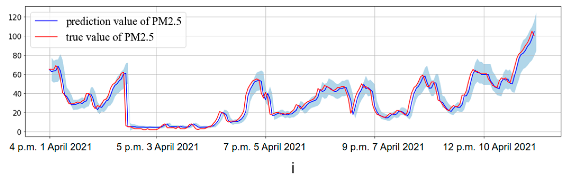
Forecast PM2.5 concentration. The samples resulting from the prediction range will be predicted via the FOSSA–DeepAR model, then we can obtain the point and interval prediction result. In addition, the prediction results will be compared with true values.

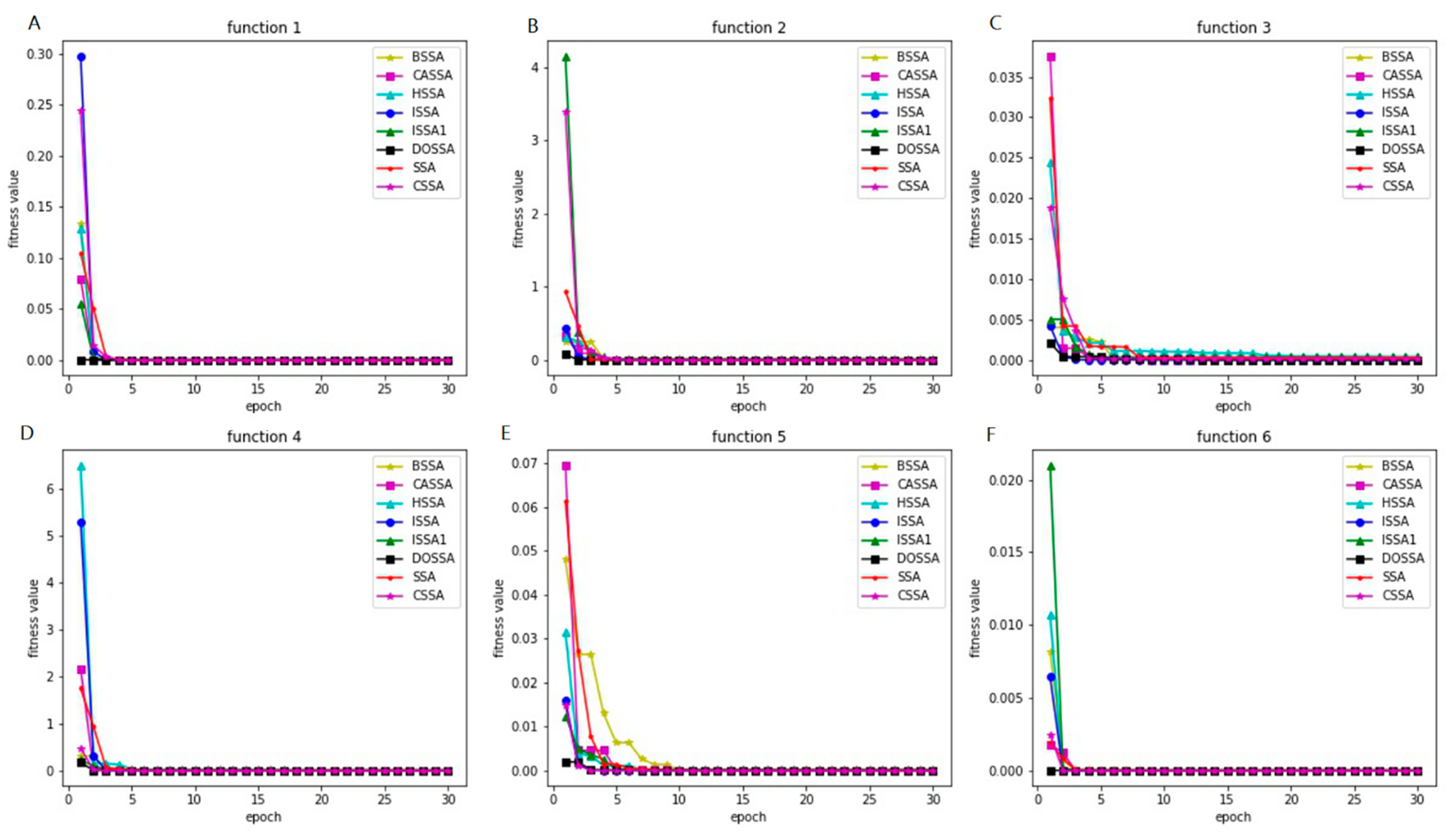
2.5. Comparison of SSA-Based Algorithms

In this subsection, according to six different benchmark functions shown in

Table 1. Benchmark functions: $f_1–f_3$ are unimodal functions and $f_4–f_6$ are multimodal functions.

Function	Range	Optimal	Dimension
$f_1={\displaystyle {\displaystyle \sum }_{i=1}^n}{x}_i^2$	${\left[-100,100\right]}^n$	0	30
$f_2={\displaystyle {\displaystyle \sum }_{i=1}^n}\left|x_i\right|+{\displaystyle {\displaystyle \prod }_{i=1}^n}\left|x_i\right|$	${\left[-10,10\right]}^n$	0	30
$f_3=\max \left\{\left|x_i\right|,1\le i\le n\right\}$	${\left[-100,100\right]}^n$	0	30
$f_4={\displaystyle {\displaystyle \sum }_{i=1}^n}\left[x_i^2-10\cos \left(2\mathsf{\pi }{x}_i\right)+10\right]$	${\left[-5.12,5.12\right]}^n$	0	30
$f_5=-20\exp \left(-0.2\sqrt{\frac{1}{n}{\displaystyle {\displaystyle \sum }_{i=1}^n}{x}_i^2}\right)-\exp \left(\frac{1}{n}{\displaystyle {\displaystyle \sum }_{i=1}^n}\cos \left(2\mathsf{\pi }{x}_i\right)\right)+20+\mathrm{e}$	${\left[-32,32\right]}^n$	0	30
$f_6=\frac{1}{4000}{\displaystyle {\displaystyle \sum }_{i=1}^n}{x}_i^2-{\displaystyle {\displaystyle \prod }_{i=1}^n}\cos \left(\frac{x_i}{\sqrt{i}}\right)+1$	${\left[-600,600\right]}^n$	0	30

, we compare the performance of FOSSA with other existing improved algorithms of SSA. Unimodal functions only have the global optimum, thus can be used to verify the basic search ability and convergence speed of the algorithm. Conversely, multimodal functions not only have the global optimum, but also the local optimum. Accordingly, they can be used to test the ability of global search. According to [10,23], the dimension of benchmark functions is set to 30.

The experiments are implemented with Spyder (anaconda) running on a PC with Inter (R) Core (TM). The packages used are NumPy and pandas.

The solutions of the optimization algorithms have randomness. Thus, the algorithms run 50 times independently in this study. The maximum number of iterations is set to 30, and the population size is set to 100. In all optimization algorithms, the alarm threshold is 0.8. Here, 10% of the individuals in the population detect danger signals and issue alarm. Except for FOSSA, 20% of individuals of other algorithms are producers, and scroungers account for 80% of the total population.

Table 2. Compared results of algorithms for unimodal functions.

		FOSSA	SSA [10]	ISSA [14]	ISSA1 * [19]	HSSA [16]	CASSA [15]	CSSA [17]	BSSA [18]
$f_1$	Min	0.0000	1.2832$\times {10}^{-11}$	6.5350$\times {10}^{-54}$	1.8723$\times {10}^{-10}$	4.0926$\times {10}^{-12}$	9.3945$\times {10}^{-16}$	2.6205$\times {10}^{-16}$	2.7542$\times {10}^{-11}$
	Max	0.0000	2.0067$\times {10}^{-5}$	7.6709$\times {10}^{-37}$	4.0530$\times {10}^{-5}$	4.9072$\times {10}^{-7}$	7.4786$\times {10}^{-7}$	1.0377$\times {10}^{-6}$	4.0879$\times {10}^{-6}$
	Mean	0.0000	1.2283$\times {10}^{-6}$	1.6564$\times {10}^{-38}$	3.1881$\times {10}^{-6}$	5.9980$\times {10}^{-8}$	7.0295$\times {10}^{-8}$	1.0301$\times {10}^{-7}$	3.9100$\times {10}^{-7}$
	Std	0.0000	3.2764$\times {10}^{-6}$	1.0734$\times {10}^{-37}$	7.2891$\times {10}^{-6}$	1.1877$\times {10}^{-7}$	1.6261$\times {10}^{-7}$	2.0642$\times {10}^{-7}$	8.4509$\times {10}^{-7}$
$f_2$	Min	0.0000	3.7571$\times {10}^{-7}$	9.1651$\times {10}^{-27}$	8.3980$\times {10}^{-7}$	1.5489$\times {10}^{-9}$	2.7173$\times {10}^{-10}$	2.4890$\times {10}^{-7}$	3.0233$\times {10}^{-7}$
	Max	0.0000	0.0032	1.5011$\times {10}^{-18}$	0.0042	0.0001	0.0009	0.0027	0.0044
	Mean	0.0000	0.0007	7.1462$\times {10}^{-20}$	0.0008	1.8077$\times {10}^{-5}$	7.5227$\times {10}^{-5}$	0.0002	0.0005
	Std	0.0000	0.0008	2.8116$\times {10}^{-19}$	0.0009	2.2011$\times {10}^{-5}$	0.0002	0.0005	0.0010
$f_3$	Min	0.0000	6.0371$\times {10}^{-6}$	4.9501$\times {10}^{-29}$	5.9852$\times {10}^{-7}$	2.6545$\times {10}^{-7}$	3.6010$\times {10}^{-14}$	1.4181$\times {10}^{-13}$	4.7708$\times {10}^{-7}$
	Max	0.0000	0.0013	2.2001$\times {10}^{-19}$	0.0016	0.0007	0.0002	0.0002	0.0010
	Mean	0.0000	0.0002	7.1001$\times {10}^{-21}$	0.0003	0.0001	8.9555$\times {10}^{-6}$	4.3154$\times {10}^{-5}$	0.0001
	Std	0.0000	0.0003	3.2061$\times {10}^{-20}$	0.0003	0.0002	3.3462$\times {10}^{-5}$	5.4241$\times {10}^{-5}$	0.0002

* The ISSA1 shown in Table 2 represents the improved sparrow search algorithm proposed in [21].

and

Table 3. Compared results of algorithms for multimodal functions.

		FOSSA	SSA [10]	ISSA [14]	ISSA1 [19]	HSSA [16]	CASSA [15]	CSSA [17]	BSSA [18]
$f_4$	Min	0.0000	4.9378$\times {10}^{-10}$	0.0000	5.5509$\times {10}^{-10}$	7.6739$\times {10}^{-13}$	0.0000	0.0000	2.8599$\times {10}^{-13}$
	Max	0.0000	0.0010	0.0000	0.0046	1.2333$\times {10}^{-5}$	0.0007	0.0003	0.0010
	Mean	0.0000	2.7938$\times {10}^{-5}$	0.0000	0.0003	8.9170$\times {10}^{-7}$	4.6639$\times {10}^{-5}$	2.6021$\times {10}^{-5}$	4.2719$\times {10}^{-5}$
	Std	0.0000	0.0001	0.0000	0.0009	2.6570$\times {10}^{-6}$	0.0001	7.3961$\times {10}^{-5}$	0.0002
$f_5$	Min	4.4409$\times {10}^{-16}$	1.2970$\times {10}^{-6}$	4.4409$\times {10}^{-16}$	5.0758$\times {10}^{-6}$	5.8863$\times {10}^{-8}$	9.9920$\times {10}^{-7}$	6.2466$\times {10}^{-7}$	8.6839$\times {10}^{-8}$
	Max	4.44089$\times {10}^{-16}$	0.0025	4.4409$\times {10}^{-16}$	0.0021	0.0002	0.0001	0.0007	0.0008
	Mean	4.4409$\times {10}^{-16}$	0.0002	4.4409$\times {10}^{-16}$	0.0003	2.0866$\times {10}^{-5}$	1.5892$\times {10}^{-5}$	9.2232$\times {10}^{-5}$	0.0002
	Std	0.0000	0.0004	0.0000	0.0004	3.4949$\times {10}^{-5}$	2.8091$\times {10}^{-5}$	0.0001	0.0002
$f_6$	Min	0.0000	1.1925$\times {10}^{-11}$	0.0000	9.9737$\times {10}^{-12}$	2.2204$\times {10}^{-16}$	0.0000	0.0000	4.7729$\times {10}^{-13}$
	Max	0.0000	1.8262$\times {10}^{-6}$	0.0000	1.2323$\times {10}^{-5}$	2.3328$\times {10}^{-7}$	1.4312$\times {10}^{-7}$	3.6241$\times {10}^{-7}$	1.2347$\times {10}^{-6}$
	Mean	0.0000	1.2497$\times {10}^{-7}$	0.0000	1.1063$\times {10}^{-6}$	1.4002$\times {10}^{-8}$	3.6135$\times {10}^{-9}$	2.1757$\times {10}^{-8}$	9.1045$\times {10}^{-8}$
	Std	0.0000	2.9969$\times {10}^{-7}$	0.0000	2.4449$\times {10}^{-6}$	3.8204$\times {10}^{-8}$	2.0267$\times {10}^{-8}$	6.2499$\times {10}^{-8}$	2.2412$\times {10}^{-7}$

show the results of the optimization algorithms on unimodal functions and multimodal functions, respectively. The four parameters shown in Table 2 and Table 3 are the minimum, maximum, mean, and variance of the optimization results. For the unimodal functions, FOSSA can find the global optimal value of $f_1$, $f_2$, $f_3$, but the other seven algorithms cannot find the global optimal solution. FOSSA can achieve better solutions in fewer iterations. Based on the statistics, the values of standard deviation, maximum, minimum, and mean of FOSSA are the smallest. Hence, the proposed FOSSA can improve the accuracy and stability of SSA. ISSAs1, ISSA1, and SSA have the poorest performance of $f_1$, $f_2$, and $f_3$, respectively.

In the experiment of multimodal function, FOSSA can give the best solution. For all multimodal functions, the four parameters of FOSSA and ISSA are smallest, which can indicate that the two algorithms achieve best performance. In general, ISSA1 has the worst performance among eight algorithms.

As shown in Figure 3, the fitness value of initial population of FOSSA is smallest, which can indicate that the quality of the initial population of FOSSA is best among all algorithms. The opposition-based learning can significantly improve the quality of the initial population than random initialization and chaotic mapping initialization. In addition, the convergence speed of FOSSA is the fastest. It can illustrate that opposition-based learning, Lévy flight, and fitness-based learning can improve searching speed and avoid getting stuck in local optimal solutions. As a result, these advantages of FOSSA can raise the accuracy of the final result.

3. Empirical Results and Analysis

In this section, we will use FOSSA–DeepAR model to make point prediction and interval prediction for PM2.5. Hourly PM2.5 concentration data observed at the Huairou monitoring station of Beijing is applied in this paper. The experiments are implemented with Spyder (anaconda) and Tensorflow running on a PC with Inter (R) Core (TM).

3.1. Data Set and Evaluation Criteria

In this paper, we use PM2.5 concentration data of the past twenty four hours to predict the PM2.5 concentration an hour later in the future. These hourly PM2.5 concentration time series are collected from 1 January 2020 to 10 April 2021. Specifically, these datasets contain two subsets: training dataset from 1 January 2020 to 3 p.m. on 1 April 2021 for establishing FOSSA–DeepAR model and test dataset from 4 p.m. 1 April 2021 to 23 p.m. 10 April 2021 for verifying the predicting performance of FOSSA–DeepAR. The time series of PM2.5 concentration is shown in Figure 4. The recurrent neural network (RNN) used in DeepAR is the long short-term memory (LSTM) model. After the training process, sample size generated by the model is set to 300, and the point prediction value of time t is the mean value of the 300 samples. Moreover, the variance of 300 samples is assumed as variance value at time t.

To evaluate the prediction ability of the FOSSA–DeepAR model for PM2.5 concentration, several statistical indices are employed in this work. These performance metrics, including Theil’s coefficient (TIC), root mean square error (RMSE), mean absolute error (MAE), mean absolute percentage error (MAPE), and $R^2$, are used to evaluate the point prediction performance. IF coverage probability and IF normalized average width is introduced to evaluate the interval prediction performance. The statistical indices are calculated as Equations (20)–(26).

$$\mathrm{TIC}=\frac{\sqrt{\frac{1}{T}{{\displaystyle \sum }}_{t=1}^T{\left(Z\left(t\right)-\widehat{Z}\left(t\right)\right)}^2}}{\sqrt{\frac{1}{T}{{\displaystyle \sum }}_{t=1}^T{Z}^2\left(t\right)}\sqrt{\frac{1}{T}{{\displaystyle \sum }}_{t=1}^T{\widehat{Z}}^2\left(t\right)}} ,$$

(20)

$$\mathrm{RMSE}=\sqrt{\frac{1}{T}{\displaystyle \sum }_{t=1}^T{\left(\widehat{Z}\left(t\right)-Z\left(t\right)\right)}^2},$$

(21)

$$\mathrm{MAE}=\frac{1}{T}{\displaystyle \sum }_{t=1}^T\left|\widehat{Z}\left(t\right)-Z\left(t\right)\right| ,$$

(22)

$$\mathrm{MAPE}=\frac{1}{T}{\displaystyle \sum }_{t=1}^T\left|\frac{\widehat{Z}\left(t\right)-Z\left(t\right)}{Z\left(t\right)}\right|\times 100\% ,$$

(23)

$$R^2=1-\frac{{{\displaystyle \sum }}_{t=1}^T{\left(\widehat{Z}\left(t\right)-Z\left(t\right)\right)}^2}{{{\displaystyle \sum }}_{t=1}^T{\left(Z\left(t\right)-\overline{Z}\right)}^2} ,$$

(24)

$$\mathrm{IFCP}=\frac{1}{T}{\displaystyle \sum }_{t=1}^T{c}_t , c_t=\{\begin{array}{c}1 , \mathrm{if} \widehat{Z}\left(t\right)\in \left(L_t,U_t\right)\\ 0 , \mathrm{otherwise}\end{array},$$

(25)

$$\mathrm{IFNAW}=\frac{1}{T}{\displaystyle \sum }_{t=1}^T\left(U_t-L_t\right)/\left(Z_{\max }-Z_{\min }\right) ,$$

(26)

where the T is the number of samples for testing, $\widehat{Z}\left(t\right)$and $Z\left(t\right)$ are the prediction value and true value of time t, respectively, $\overline{Z}$ is the mean value of time series, and $U_t$ and $L_t$ are the upper and lower bounds of the prediction interval, respectively. The smaller value of TIC, RMSE, MAE, MAPE, and IFNAW mean lower prediction bias and better prediction performance. The higher values of IFCP and $R^2$ mean superior prediction performance.

3.2. Results and Analysis

In order to show the effectiveness of FOSSA–DeepAR model, we use eight benchmark models including DeepAR, SSA–DeepAR, BSSA–DeepAR, CASSA–DeepAR, CSSA–DeepAR, HSSA–DeepAR, ISSA–DeepAR, and ISSA1–DeepAR.

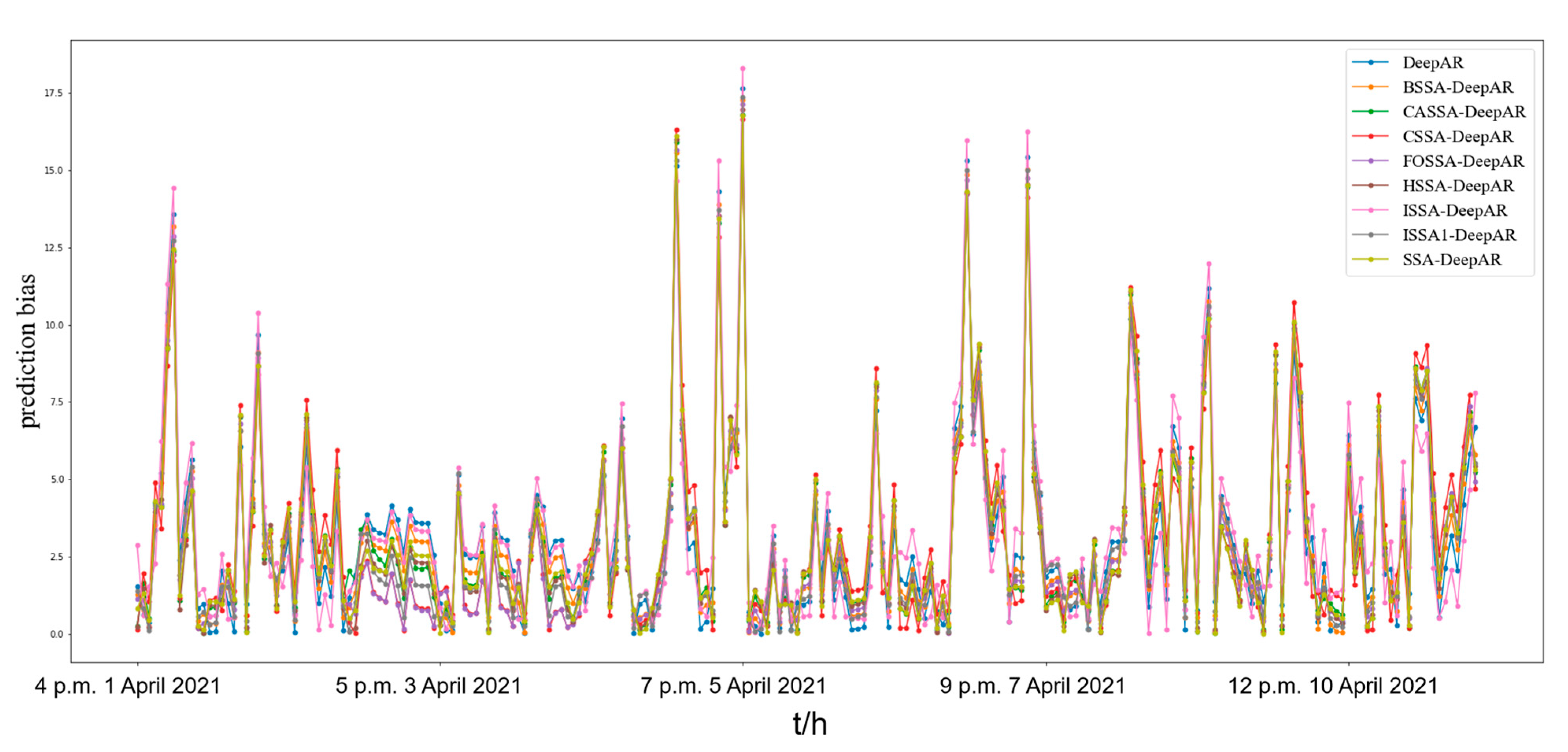
3.2.1. Prediction of PM2.5 Concentration in Beijing

Figure 5 and Figure 6 show point prediction values and absolute bias values of PM2.5 concentration, respectively. Point prediction errors of FOSSA–DeepAR are smallest in nine models. Compared to the DeepAR model, the RMSE, MAE, and MAPE of FOSSA–DeepAR are reduced by 5.77%, 10.39%, and 51.7%, respectively. The single DeepAR model has the poorest performance for PM2.5 concentration among the forecasting models. The proposed FOSSA–DeepAR achieves the best performance for point prediction.

Table 4. Statistical indices of PM2.5 concentration prediction in Beijing.

Model	Statistical Indicator
	TIC*100	RMSE	MAE	MAPE(%)	${\mathit{R}}^2$	IFCP	IFNAW
FOSSA–DeepAR	0.3619	5.6242	3.2011	18.9297	0.9322	0.8744	0.1108
BSSA–DeepAR	0.3710	5.8841	3.5232	21.0970	0.9258	0.7444	0.1266
CASSA–DeepAR	0.3730	5.7583	3.4411	23.2321	0.9290	0.7534	0.1236
CSSA–DeepAR	0.3647	5.7484	3.2691	20.4574	0.9300	0.7534	0.1187
HSSA–DeepAR	0.3659	5.7136	3.3003	22.8887	0.9300	0.7758	0.1312
ISSA–DeepAR	0.3667	5.9316	3.5164	28.6855	0.9246	0.7713	0.1310
ISSA1–DeepAR	0.3635	5.7102	3.3062	22.0377	0.9201	0.7175	0.1206
SSA–DeepAR	0.3686	5.7412	3.3620	23.6472	0.9294	0.7354	0.1178
DeepAR	0.3757	5.9485	3.5337	28.7165	0.9205	0.7265	0.1230

shows the evaluation indices of different models for point prediction of PM2.5 concentration. From Table 4, we see that the forecasting accuracy of the nine models are different. TIC, RMSE, MAE, and MAPE of the FOSSA–DeepAR model are lower than other hybrid models and the single DeepAR model. At the same time, $R^2$ of FOSSA–DeepAR is higher than other models. Accordingly, FOSSA–DeepAR outperforms other hybrid models and the single model for point prediction of PM2.5 concentration. Compared with a single DeepAR model, FOSSA–DeepAR model can reduce the RMSE of point prediction by an average of 5.76%, MAE by an average 10.39%, and MAPE by average 9.76%. In addition, compared with other hybrid models, FOSSA–DeepAR reduces the RMSE, MAE, and MAPE by an average of 2.834%, 6.243%, and 22.55%, respectively. In addition, the $R^2$ of FOSSA–DeepAR is 0.93 and is higher than other benchmark models. The FOSSA–DeepAR model has better model fitting capability and more accurate point prediction. For the interval prediction, IFCP of FOSSA–DeepAR is 14.79% higher than the DeepAR, 16.63% higher than other hybrid models, on average. FOSSA has a better performance for optimizing the initial weight of the DeepAR model. FOSSA can significantly improve the prediction accuracy of DeepAR.

Figure 7 shows the interval prediction results PM2.5 concentration. The blue shaded area is the interval prediction of PM2.5 concentration. Higher IFCP means a stronger interval prediction ability of model. In addition, the lower IFNAW indicates a higher accuracy of interval prediction. The minimum value of IFCP is 0.7175, which is 21.87% lower than FOSSA–DeepAR. ISSA1–DeepAR has the poorest performance for interval prediction. The proposed FOSSA–DeepAR can improve the interval prediction performance of PM2.5 concentration.

To further demonstrate the forecasting ability of the proposed FOSSA–DeepAR model, Diebold–Mariano hypothesis test [24] is utilized to verify that the prediction results of FOSSA–DeepAR are significantly different from the results of another benchmark models. In other words, the significance difference represents the difference in model prediction performance. According to the results shown in

Table 5. DM test results of PM2.5 concentration point forecasting results in Beijing.

Tested Model	Benchmark Model
	BSSA–DeepAR	CASSA–DeepAR	CSSA–DeepAR	HSSA–DeepAR	ISSA–DeepAR	ISSA1–DeepAR	SSA–DeepAR	DeepAR
FOSSA–DeepAR	2.9466 (0.0032)	7.4423 (9.8810 $\times {10}^{-14}$)	2.5708 (0.0101)	4.0025 (6.2684 $\times {10}^{-5}$)	4.2075 (2.5816 $\times {10}^{-5}$)	6.6270 (3.4248 $\times {10}^{-11}$)	3.2962 (0.0009)	3.0460 (0.0023)
BSSA–DeepAR		0.7494 (0.4536)	1.9894 (0.0467)	1.8231 (0.0683)	2.0038 (0.0451)	1.8455 (0.0650)	1.8861 (0.0593)	2.1990 (0.0279)
CASSA–DeepAR			4.2459 (2.1771 $\times {10}^{-5}$)	1.2799 (0.2006)	2.1025 (0.0355)	0.1172 (0.9067)	1.7705 (0.0766)	4.6478 (3.3555 $\times {10}^{-6}$)
CSSA–DeepAR				5.4134 (6.1825 $\times {10}^{-8}$)	6.8126 (9.5870 $\times {10}^{-12}$)	3.0353 (0.0024)	1.5721 (0.1159)	3.0350 (0.0024)
HSSA–DeepAR					2.0132 (0.0441)	1.2393 (0.2152)	3.6971 (0.0002)	2.0012 (0.0454)
ISSA–DeepAR						1.6791 (0.0931)	3.3655 (0.0008)	2.6089 (0.0091)
ISSA1–DeepAR							7.4389 (1.0147 $\times {10}^{-13}$)	6.8539 (7.1887 $\times {10}^{-12}$)
SSA–DeepAR								3.0672 (0.0022)

, all SSA-based algorithms can reinforce the prediction performance of DeepAR. However, compared with other hybrid models, the result of FOSSA–DeepAR has a significant difference. The result means that FOSSA–DeepAR model has a more effective forecasting ability. FOSSA–DeepAR outperforms other hybrid models and single model as the initial weights of DeepAR are optimized significantly by FOSSA.

3.2.2. Robustness Analysis of FOSSA–DeepAR

To further show the stability of FOSSA–DeepAR, this proposed model is applied to predict PM2.5 concentration and O₃ concentration observed by Taian monitoring station in Shandong, O₃ concentration observed by Huairou monitoring station in Beijing. For the conditioning range and prediction range, the last 200 time points of each time series will be used as the prediction range, and other time series are used to train the model.

Table 6. Statistical indices of prediction of O₃ in Beijing, and PM2.5 and O₃ in Taian.

Time Series	Statistical Indicator
	TIC	RMSE	MAE	MAPE	${\mathit{R}}^2$	IFCP	IFNAW
O3 in Beijing	0.0012	7.9824	5.9910	0.0939	0.9005	0.8350	0.1996
PM2.5 in Taian	0.0013	14.1004	10.1996	0.3797	0.9182	0.7750	0.2390
O3 in Taian	0.0029	9.3287	6.1833	0.1993	0.9132	0.7750	0.2065

gives the evaluation indices of FOSSA–DeepAR model for PM2.5 prediction. For point prediction of PM2.5, the average value of TIC, RMSE, MAE, and MAPE are 0.0024, 9.8623, 6.7003, and 28.45%, respectively. RMSE, MAE, and MAPE in Taian are higher due to higher PM2.5 concentration. The average value of $R^2$ is 0.9252. This means FOSSA–DeepAR achieves good point prediction for PM2.5 in Beijing and Taian. In addition, for interval prediction, the average value of IFCP and IFNAW are 0.8247 and 0.1749, respectively. This means 82.47% of true values are included in the interval prediction. FOSSA–DeepAR model also achieves good interval prediction for PM2.5 in Beijing and Taian. For O₃ concentration, the average value of TIC, RMSE, MAE, MAPE, $R^2$, IFCP, and IFNAW are 0.0021, 8.6106, 6.0872, 14.66%, 0.9069, 0.805, and 0.2031, respectively. This shows that FOSSA–DeepAR also provides a good prediction for O₃ concentration.

Figure 8, Figure 9 and Figure 10 show the interval prediction of O₃ concentration in Beijing, PM2.5 concentration in Taian, and O₃ concentration in Taian, respectively. Most of the true values of atmospheric concentration are included in the interval prediction. The range of interval prediction is small, which means the accuracy of interval prediction is good. Accordingly, the proposed FOSSA–DeepAR model can be utilized for different atmospheric concentration and different regions.

4. Conclusions and Future Research

In this paper, a hybrid learning approach based on FOSSA and DeepAR is proposed to obtain the point and interval prediction of the PM2.5 concentration. In this paper, a novel hybrid learning approach based on FOSSA and DeepAR is proposed to simultaneously obtain point and interval predictions of PM2.5 concentration. Firstly, driven by the ABC algorithm, we use fitness-based learning, opposition-based learning, and Lévy flight to improve SSA, which outperforms other existing SSA-based algorithms. Thus, we introduce the DeepAR model into the field of air quality prediction, and use the proposed FOSSA to optimize DeepAR. Consequently, a FOSSA–DeepAR learning method is established. Moreover, we use the FOSSA–DeepAR hybrid learning method to predict PM2.5 and O3 concentration in Beijing and Taian. The empirical results show the powerful optimization capabilities of FOSSA, and the outstanding prediction performance of FOSSA–DeepAR.

We know that PM2.5 concentration is affected by many factors, such as air humidity, air pressure, and landforms, etc. These factors are not considered in this paper, which is a limitation. In future work, we will pay close attention to covariate time series in the FOSSA–DeepAR model. We will also take into account the prediction capability of the proposed model in different areas and countries, such as Brazil and Mexico. Other probability can also be utilized in the FOSSA–DeepAR model.

References

1. Zhang, L.; Lin, J.; Qiu, R.; Hu, X.; Zhang, H.; Chen, Q.; Tan, H.; Lin, D.; Wang, J. Trend analysis and forecast of PM2.5 in Fuzhou, China using the ARIMA model. Ecol. Indic. 2018, 95, 702–710. [Google Scholar] [CrossRef]
2. Cavieres, M.F.; Leiva, V.; Marchant, C.; Rojas, F. A Methodology for Data-Driven Decision-Making in the Monitoring of Particulate Matter Environmental Contamination in Santiago of Chile. Rev. Environ. Contam. Toxicol. 2020, 250, 45–67. [Google Scholar] [CrossRef]
3. Puentes, R.; Marchant, C.; Leiva, V.; Figueroa-Zúñiga, J.; Ruggeri, F. Predicting PM2.5 and PM10 Levels during Critical Episodes Management in Santiago, Chile, with a Bivariate Birnbaum-Saunders Log-Linear Model. Mathematics 2021, 9, 645. [Google Scholar] [CrossRef]
4. Jiang, F.; He, J.; Zeng, Z. Pigeon-inspired optimization and extreme learning machine via wavelet packet analysis for predicting bulk commodity futures prices. Sci. China Inf. Sci. 2019, 62, 70204. [Google Scholar] [CrossRef] [Green Version]
5. Wong, P.-Y.; Lee, H.-Y.; Chen, Y.-C.; Zeng, Y.-T.; Chern, Y.-R.; Chen, N.-T.; Lung, S.-C.C.; Su, H.-J.; Wu, C.-D. Using a land use regression model with machine learning to estimate ground level PM2.5. Environ. Pollut. 2021, 277, 116846. [Google Scholar] [CrossRef] [PubMed]
6. Lu, X.; Sha, Y.H.; Li, Z.; Huang, Y.; Chen, W.; Chen, D.; Shen, J.; Chen, Y.; Fung, J.C. Development and application of a hybrid long-short term memory—Three dimensional variational technique for the improvement of PM2.5 forecasting. Sci. Total Environ. 2021, 770, 144221. [Google Scholar] [CrossRef]
7. Jiang, F.; Qiao, Y.; Jiang, X.; Tian, T. MultiStep Ahead Forecasting for Hourly PM10 and PM2.5 Based on Two-Stage Decomposition Embedded Sample Entropy and Group Teacher Optimization Algorithm. Atmosphere 2021, 12, 64. [Google Scholar] [CrossRef]
8. Huang, G.; Li, X.; Zhang, B.; Ren, J. PM2.5 concentration forecasting at surface monitoring sites using GRU neural network based on empirical mode decomposition. Sci. Total Environ. 2021, 768, 144516. [Google Scholar] [CrossRef]
9. Jiang, F.; He, J.; Tian, T. A clustering-based ensemble approach with improved pigeon-inspired optimization and extreme learning machine for air quality prediction. Appl. Soft Comput. 2019, 85, 105827. [Google Scholar] [CrossRef]
10. Xue, J.; Shen, B. A novel swarm intelligence optimization approach: Sparrow search algorithm. Syst. Sci. Control. Eng. 2020, 8, 22–34. [Google Scholar] [CrossRef]
11. Clerc, M. Particle Swarm Optimization; Ashgate: Farnham, UK, 2006. [Google Scholar]
12. Song, X.; Tang, L.; Zhao, S.; Zhang, X.; Li, L.; Huang, J.; Cai, W. Grey Wolf Optimizer for parameter estimation in surface waves. Soil Dyn. Earthq. Eng. 2015, 75, 147–157. [Google Scholar] [CrossRef]
13. Rashedi, E.; Nezamabadi-Pour, H.; Saryazdi, S. GSA: A Gravitational Search Algorithm. Inf. Sci. 2009, 179, 2232–2248. [Google Scholar] [CrossRef]
14. Yuan, J.; Zhao, Z.; Liu, Y.; He, B.; Wang, L.; Xie, B.; Gao, Y. DMPPT Control of Photovoltaic Microgrid Based on Improved Sparrow Search Algorithm. IEEE Access 2021, 9, 16623–16629. [Google Scholar] [CrossRef]
15. Liu, G.; Shu, C.; Liang, Z.; Peng, B.; Cheng, L. A Modified Sparrow Search Algorithm with Application in 3d Route Planning for UAV. Sensors 2021, 21, 1224. [Google Scholar] [CrossRef]
16. Li, A. Hybrid Sparrow Search Algorithm. Comput. Knowl. Technol. 2021, 17, 232–234. [Google Scholar] [CrossRef]
17. Zhang, C.; Ding, S. A stochastic configuration network based on chaotic sparrow search algorithm. Knowl.-Based Syst. 2021, 220, 106924. [Google Scholar] [CrossRef]
18. Liu, T.; Yuan, Z.; Wu, L.; Badami, B. Optimal brain tumor diagnosis based on deep learning and balanced sparrow search algorithm. Int. J. Imaging Syst. Technol. 2021. [Google Scholar] [CrossRef]
19. Lv, X.; Mu, X.; Zhang, J. Multi-threshold image segmentation based on improved sparrow search algorithm. Syst. Eng. Electr. 2021, 43, 318–327. [Google Scholar] [CrossRef]
20. Salinas, D.; Flunkert, V.; Gasthaus, J.; Januschowski, T. DeepAR: Probabilistic forecasting with autoregressive recurrent networks. Int. J. Forecast. 2020, 36, 1181–1191. [Google Scholar] [CrossRef]
21. Dong, M.; Wu, H.; Hu, H.; Azzam, R.; Zhang, L.; Zheng, Z.; Gong, X. Deformation Prediction of Unstable Slopes Based on Real-Time Monitoring and DeepAR Model. Sensors 2020, 21, 14. [Google Scholar] [CrossRef]
22. Chen, X.; Tianfield, H.; Du, W. Bee-foraging learning particle swarm optimization. Appl. Soft Comput. 2021, 102, 107134. [Google Scholar] [CrossRef]
23. Ahmadianfar, I.; Heidari, A.A.; Gandomi, A.H.; Chu, X.; Chen, H. RUN beyond the metaphor: An efficient optimization algorithm based on Runge Kutta method. Expert Syst. Appl. 2021, 181, 115079. [Google Scholar] [CrossRef]
24. Liu, Z.; Jiang, P.; Zhang, L.; Niu, X. A combined forecasting model for time series: Application to short-term wind speed forecasting. Appl. Energy 2020, 259, 114137. [Google Scholar] [CrossRef]
Figure 1. Flowchart of FOSSA. First of all, opposition-based learning is used to generate initial population for improving the quality and diversity of initial population. In addition, the Lévy flight is utilized in Equations (2) and (6). Finally, fitness-based learning is introduced into the whole searching process of sparrows.
Atmosphere 12 00894 g001
Figure 2. Process of DeepAR in conditioning range. At each time point t, the inputs of DeepAR model are x i , t , z i , t 1 and h i , t 1 , where h i , t 1 is the previous output of neural network, x i , t is the value of covariates at time t, z i , t 1 is the target value at time t−1. The value of z i , t 1 is available during conditioning range and is used to train the model. The z i , t 1 is unknown during prediction range, and z i , t 1 is replaced by z ˜ i , t 1 when DeepAR is utilized to achieve multi-step forecasts.
Atmosphere 12 00894 g002
Figure 3. Convergence curve of algorithms on unimodal functions and multimodal functions. Subgraphs (AF) represent the convergence curve of benchmark function f 1 f 6 . The quality of the initial population generated by the FOSSA algorithm is significantly higher than other algorithms. In addition, the convergence speed and search abilities of FOSSA is better than other algorithms.
Atmosphere 12 00894 g003
Figure 4. PM2.5 concentration in Beijing.
Atmosphere 12 00894 g004
Figure 5. Point prediction results and true values of PM2.5 concentration in Beijing. In the nine prediction models, the point prediction result of FOSSA–DeepAR outperforms other models.
Atmosphere 12 00894 g005
Figure 6. Prediction bias of PM2.5 concentration in Beijing. In the nine prediction models, the prediction bias of FOSSA–DeepAR is the smallest, which means FOSSA–DeepAR has best accuracy.
Atmosphere 12 00894 g006
Figure 7. Point and interval prediction of PM2.5 concentration in Beijing. Subgraphs (ai) represent the point and interval prediction result of BSSA–DeepAR, CASSA–DeepAR, CSSA–DeepAR, FOSSA–DeepAR, HSSA–DeepAR, ISSA–DeepAR, ISSA1–DeepAR, SSA–DeepAR, and DeepAR, respectively.
Atmosphere 12 00894 g007aAtmosphere 12 00894 g007b
Figure 8. Forecasting results of O3 concentration in Beijing.
Atmosphere 12 00894 g008
Figure 9. Forecasting results of PM2.5 concentration in Taian.
Atmosphere 12 00894 g009
Figure 10. Forecasting results of O3 concentration in Taian.
Atmosphere 12 00894 g010