Article

Continuous CO2 and CH4 Observations in the Coastal Arctic Atmosphere of the Western Taimyr Peninsula, Siberia: The First Results from a New Measurement Station in Dikson

1
V.N. Sukachev Institute of Forest of the Siberian Branch of Russian Academy of Sciences—Separated Department of the KSC SB RAS, 660036 Krasnoyarsk, Russia
2
Max Planck Institute for Biogeochemistry, D07745 Jena, Germany
3
Department of Forest Botany, Dendrology and Geobiocenology, Faculty of Forestry and Wood Technology, Mendel University in Brno, 61300 Brno, Czech Republic
4
Joint Directorate of Taimyr Nature Reserves, 663305 Norilsk, Russia
5
Institute for Atmospheric and Earth System Research, University of Helsinki, 00560 Helsinki, Finland
*
Author to whom correspondence should be addressed.
Atmosphere 2021, 12(7), 876; https://doi.org/10.3390/atmos12070876
Submission received: 4 June 2021 / Revised: 1 July 2021 / Accepted: 2 July 2021 / Published: 6 July 2021

Abstract

:
Atmospheric observations of sources and sinks of carbon dioxide (CO2) and methane (CH4) in the pan-Arctic domain are highly sporadic, limiting our understanding of carbon turnover in this climatically sensitive environment and the fate of enormous carbon reservoirs buried in permafrost. Particular gaps apply to the Arctic latitudes of Siberia, covered by the vast tundra ecosystems underlain by permafrost, where only few atmospheric sites are available. The paper presents the first results of continuous observations of atmospheric CO2 and CH4 dry mole fractions at a newly operated station “DIAMIS” (73.506828° N, 80.519869° E) deployed on the edge of the Dikson settlement on the western coast of the Taimyr Peninsula. Atmospheric mole fractions of CO2, CH4, and H2O are measured by a CRDS analyzer Picarro G2301-f, which is regularly calibrated against WMO-traceable gases. Meteorological records permit screening of trace gas series. Here, we give the scientific rationale of the site, describe the instrumental setup, analyze the local environments, examine the seasonal footprint, and show CO2 and CH4 fluctuations for the daytime mixed atmospheric layer that is representative over a vast Arctic domain (~500–1000 km), capturing both terrestrial and oceanic signals.

1. Introduction

Climate change in the Arctic follows a global trend, but with higher amplitudes and recorded growth of air temperature [1], more than double that of the Northern Hemisphere mean value [2], and the most notable temperature increase has been observed during colder seasons [3]. Within the past few decades, the Arctic has experienced rapid and diverse environmental alterations, such as enhanced productivity of the vegetation or the so-called “Arctic greening”, vegetation season length, and degradation of the permafrost [2,4,5,6,7]. The observed warming trend may also concern the fate of shelf environments in the Arctic Ocean characterized by the presence of subsea permafrost and associated gas hydrates buried in the sediments [8].
Higher temperatures are expected to trigger positive feedback of enlarged terrestrial releases of carbon dioxide (CO2) and methane (CH4) [9,10,11]. In a warmer climate, terrestrial uptake of CO2 may be promoted by longer vegetation season [12] and an effect of fertilization due to growing CO2 levels in the atmosphere [13]. On the other hand, the expected uptake may be counterbalanced by the rising impact of midsummer drought stress on the photosynthesis [14], enhanced microbial decomposition of soil organic matter [15], extended soil respiration period [16], and permafrost degradation with expected emissions of carbon dioxide to the atmosphere [11]. Along with CO2, the Arctic has been considered a hotspot for recent [17] and projected global-scale emissions of CH4 [16,18,19]. Enhanced thaw depths of permafrost underlain soils and thermokarst lake formation [20] are expected to mobilize vast carbon reservoirs stored in deeper soil layers by the promoted activity of methanogenic microorganisms and increase CH4 emissions to the atmosphere; however, the terms and duration of the response under projected warming remain unclear [21,22]. The effect of higher precipitation amounts in advecting thermal energy into deeper soil and increasing CH4 release is also widely discussed [23,24]. Besides the earth feedbacks, the recently observed growth of water temperatures in the coastal and inner shelf regions of the East Siberian Shelf in the Arctic Ocean [25], intense episodic warming in the central shelf sea [26], and the increasing influx of warmer Atlantic water into the Arctic Ocean (AO), or the so-called “Atlantification” [27], illustrate progressing warming that is capable of destabilizing Arctic subsea permafrost and gas hydrate reservoirs and promoting further emissions of methane [28].
Atmospheric observations of CO2 and CH4 mole fractions at masts or towers have been previously utilized for studying their releases and trends in the northern latitudes [29,30,31,32]. Such measurements deal with a large area of influence (“footprint”) as of hundreds to thousands of kilometers [33], in contrast to eddy covariance towers for carbon flux measurements, representing the local ecosystem-scale domain of a few hectares [34], or dynamic chamber technique measurements primarily used to capture homogeneous ecosystem patches (~1 m2) or individual plant communities [35]. The tower-based atmospheric measurements integrate spatially heterogeneous fluxes, but since they do not deal with direct carbon fluxes, mole fraction observations require further implementation into a model framework to infer surface-atmosphere sinks and sources. In this respect, inverse modeling of atmospheric trace gas transport is considered a powerful tool to glean insights into regional to pan-Arctic scale patterns of CO2 and CH4, including their intra- and inter-annual fluctuations and long-term trends.
Measurements of atmospheric CO2 and CH4 dry mole fractions in the pan-Arctic domain are very sparse, dramatically limiting the spatio-temporal resolution and accuracy of the models. The sporadic observations particularly concern the Arctic latitudes of Siberia, covered by the vast permafrost underlain tundra on the area of ~3 million km2, i.e., nearly half of tundra ecosystems [36]. In contrast to its global relevance for the atmospheric carbon budget, an existing observational network in these latitudes contained only a few stations continuously measuring atmospheric CO2 and CH4 (Figure 1). The recently started atmospheric measurements in the western Taimyr Peninsula at the gulf of the Yenisei River—one of the major Arctic River catchments in Siberia and Northern Eurasia [37]—fill a significant gap in the atmospheric trace gas observations over the Arctic belt of the Siberian domain. In the article, we present the first results (September 2018–February 2020) of the continuous observations of atmospheric CO2 and CH4 dry mole fractions, give the scientific rationale of the new site, describe technical details of the instrumental setup, analyze the local environments, examine the seasonal footprint, and give an overview of CO2 and CH4 fluctuations for the daytime mixed atmospheric layer that is represented throughout a large area (~500–1000 km) of the Arctic domain in Siberia, capturing carbon signatures both from the Arctic Ocean and the land surface.

2. Materials and Methods
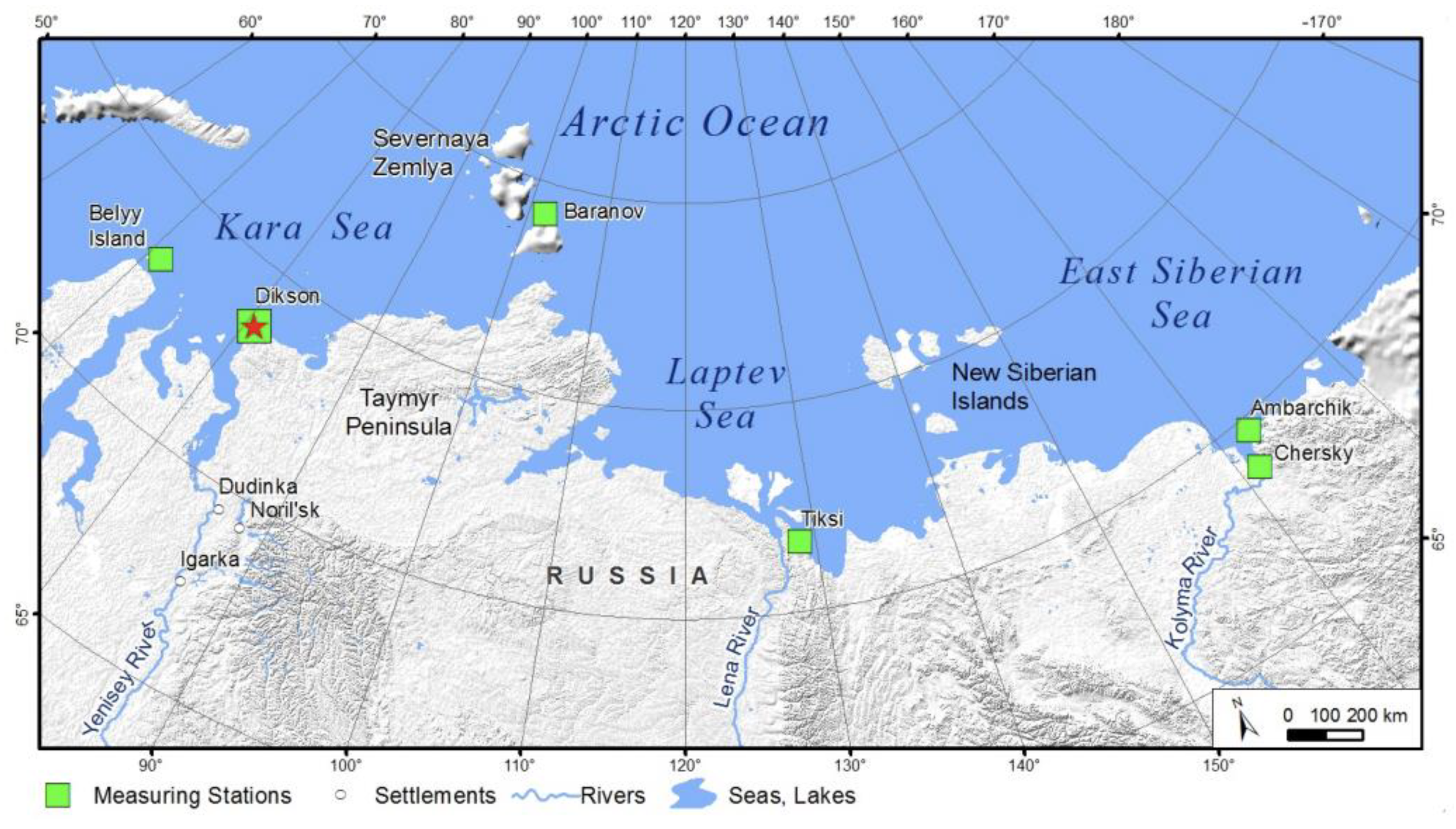
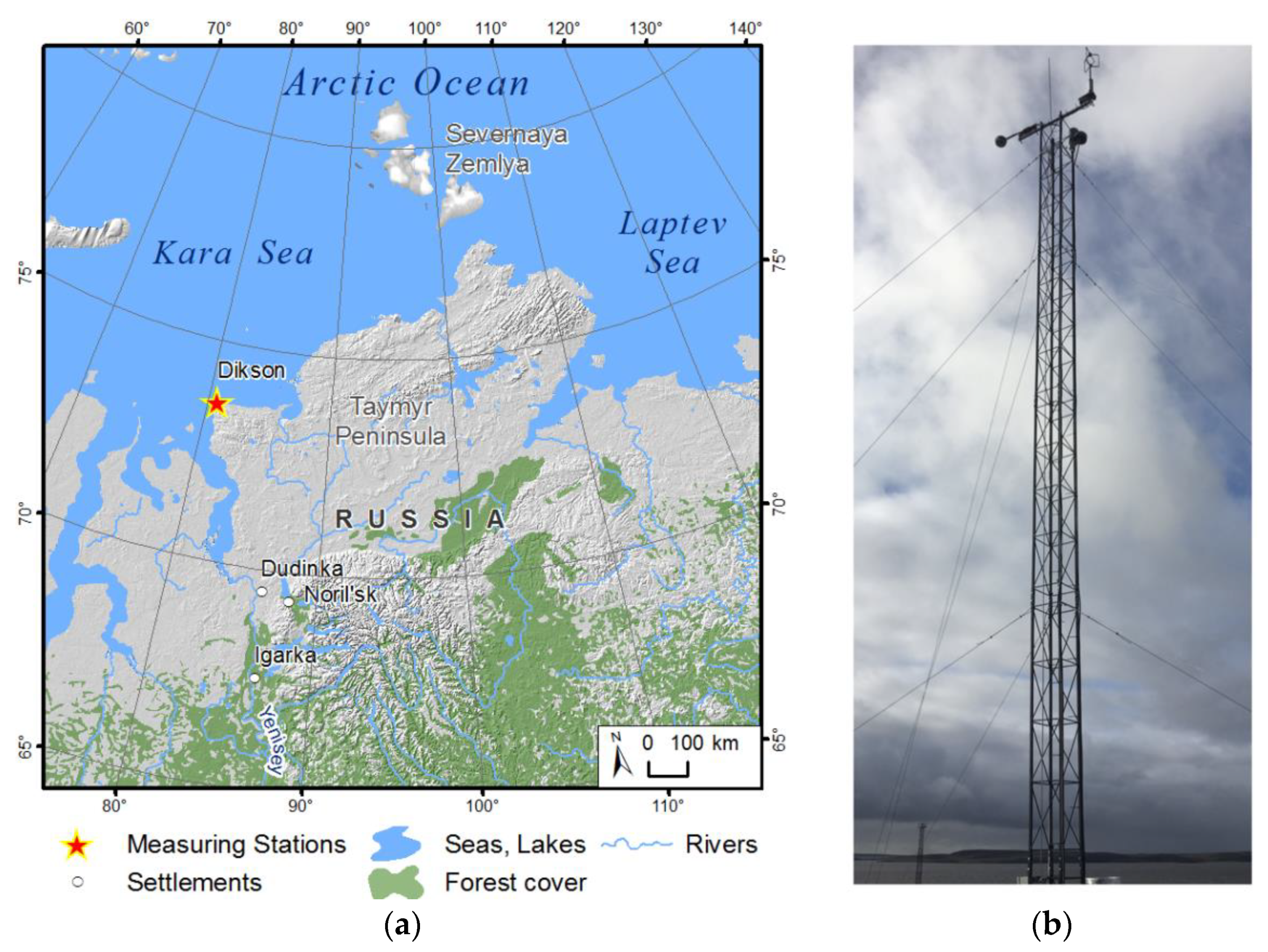
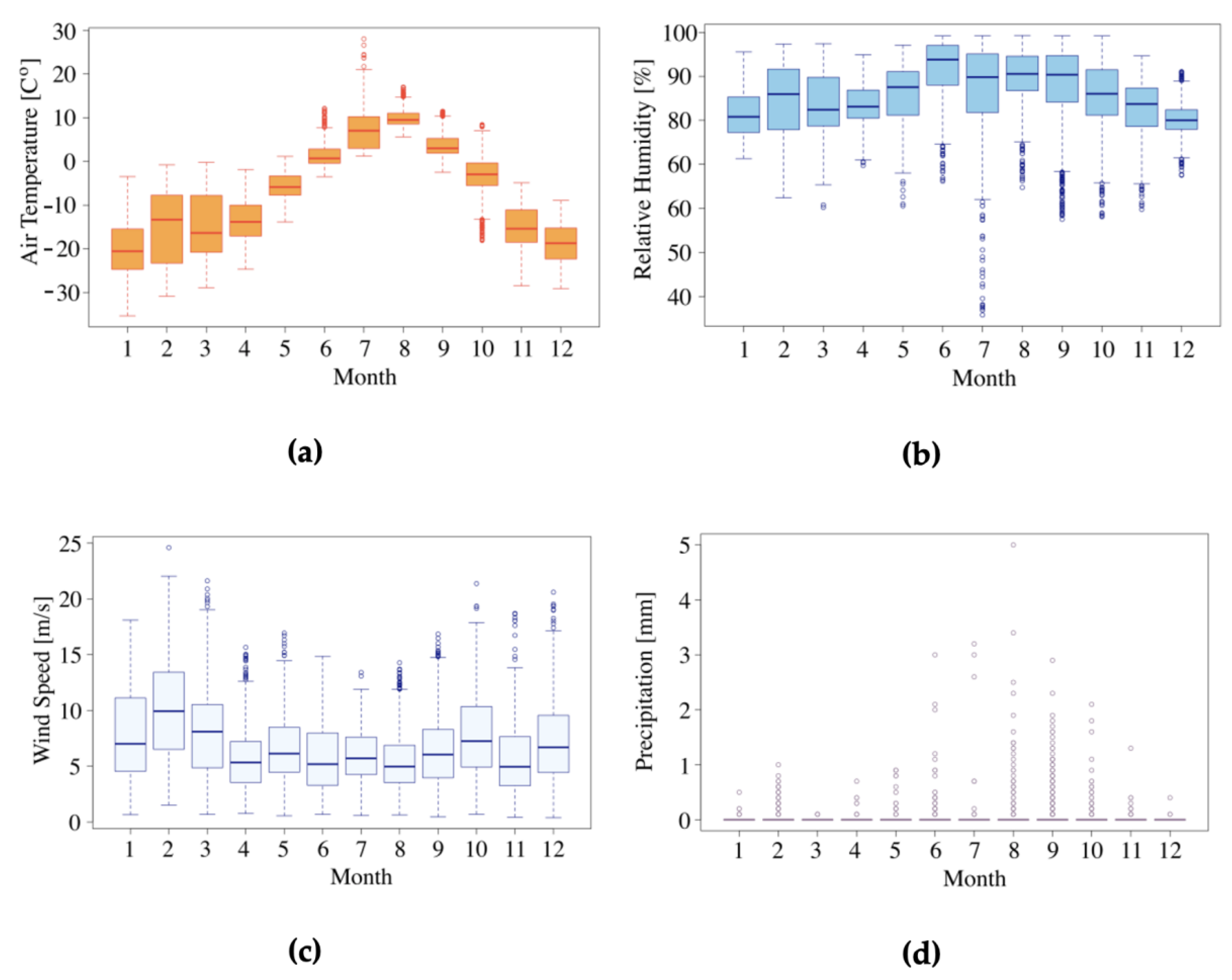
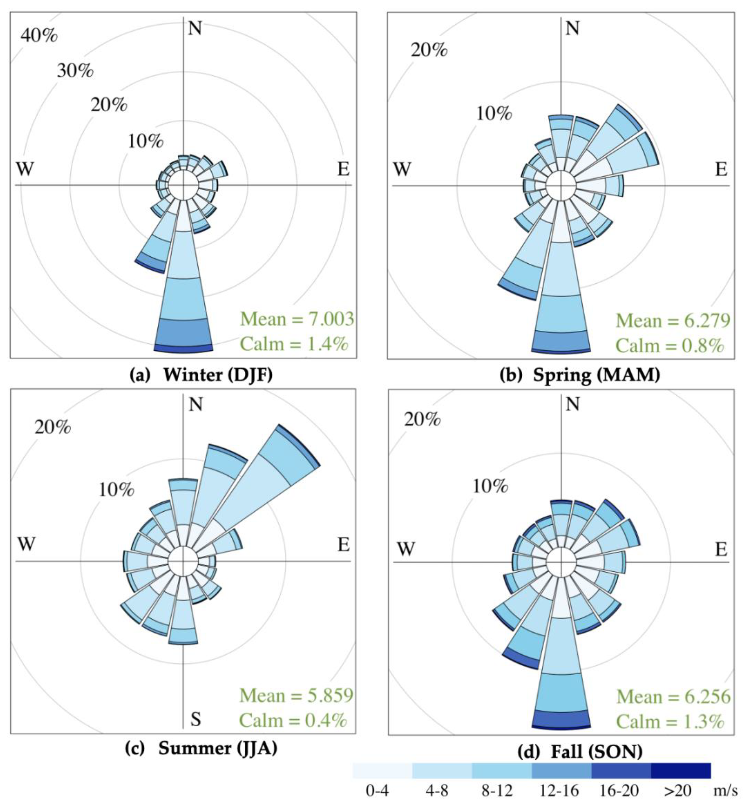
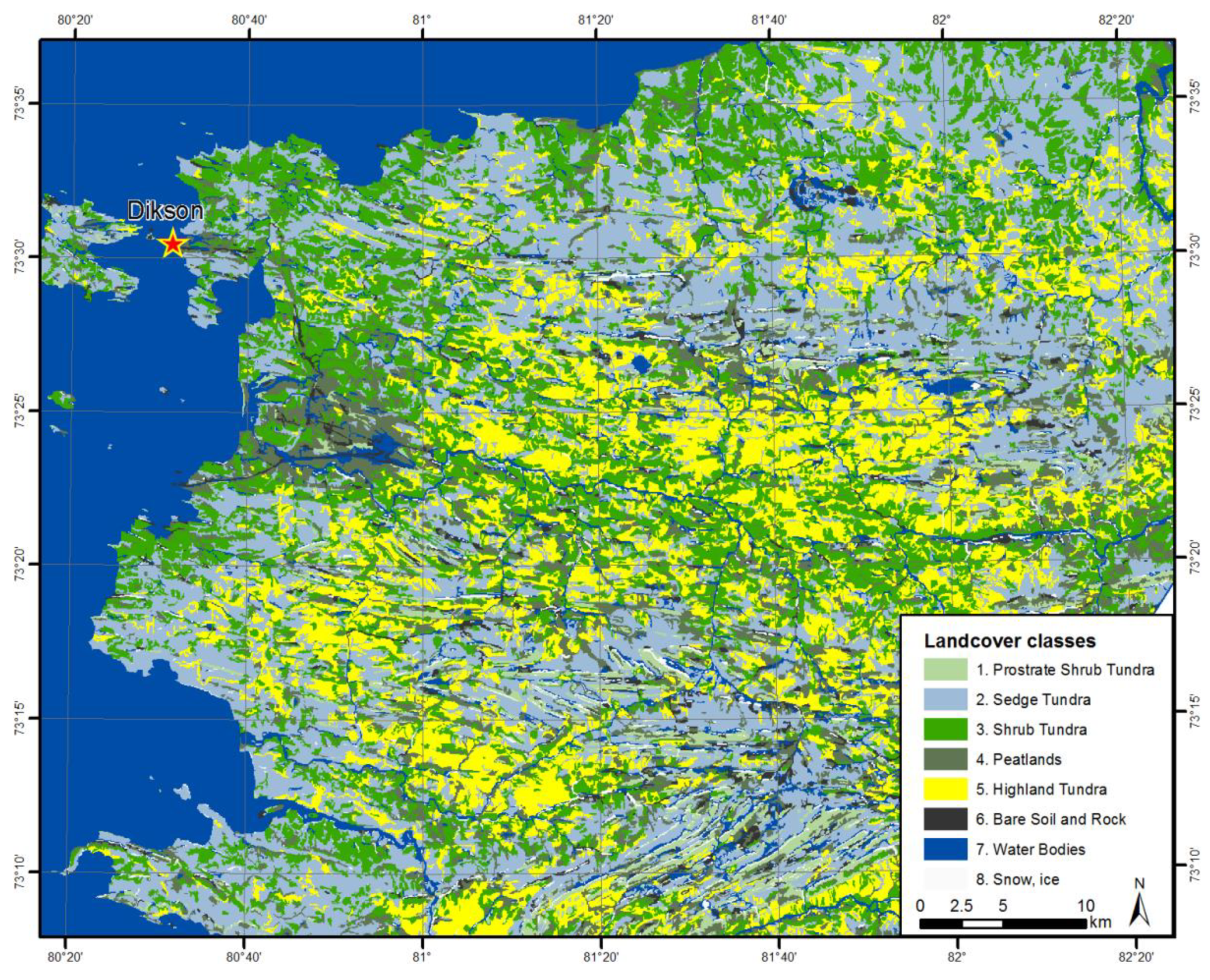
2.1. Study Area

The newly deployed measurement station “DIAMIS” (73.506828° N, 80.519869° E) is located on the edge of the Dikson settlement in the southwestern domain of the Taimyr Peninsula (Figure 2a), a northernmost extension of the Eurasian continent.
The peninsula borders the Laptev Sea and the Gulf of the Khatanga River on the east and the Kara Sea and the Gulf of the Yenisei River on the west. The Byrranga Mountains in the center of the peninsula, with elevations up to 500–1150 m and tundra-covered lowlands stretching north- and southward, define the landscape [38]. The area is relatively undisturbed and inhospitable due to the harsh climate.
Based on the Köppen climate classification [39], the study area may be characterized by a “polar” or “tundra” climate, with a marine influence observed over the coastal area where the observations are operational. The summer is short, with a mean temperature reaching +3.8 °C, while winters are relatively mild, with a mean temperature as low as −24.2 °C, and intense blizzards are particularly frequent in the area with a mean wind speed of 6.9 m/s (Figure 3). One should note that based on the Russian Federal Service for Hydrometeorology and Environmental Monitoring, the summer of 2020 demonstrated the air temperatures in the Arctic that have never achieved such high since instrumental measurements started in the year 1881, with the northern parts of the Taimyr Peninsula experiencing the most significant temperature fluctuations [40]. Even though the summer of 2020 is beyond the scope of this study, it perfectly reflects the ongoing changes particularly applied to the measurement site that captured the epicenter of the recently observed Arctic heatwave.
The analysis of multi-year wind distribution for the study area based on the longer-term data records from the weather station “The Island of Dikson” (WMO ID: 20674), located at proximity to the measurement site (3.7 km to the northwest), shows a predominance of northeast and southwest wind directions throughout the seasons (Figure 4). Winds during colder months (October–March) are mainly from the south and southwest, with some frequencies of winds blowing from northeast and southeast during fall (SON) and northeast in spring (MAM). During summer (JJA), winds prevail from the north to the northeast, with fewer frequencies from the south to the southwest.
Since single meteorological observations may be subject to strong local and regional effects, to deal with larger spatial domains and examine the source regions of air parcels moving into the study area, we developed a backward trajectory frequency analysis for the period of our observations (September 2018–February 2020). Such analysis deals with “footprint” estimates of the measurement site. For this purpose, with a daily frequency, we computed 5-day backward trajectories using the HYbrid Single-Particle Lagrangian Integrated Trajectory (HYSPLIT) model [41] from the ARL NOAA, which calculates trajectories based on a global wind and meteorology field estimation. The monthly data archives from the NCEP/NCAR Reanalysis Project (CDAS) were implemented as the driving meteorological fields for our computation. The analysis of the footprint estimates is further given in Section 3.1.
According to the Circumpolar Arctic Vegetation Map [42], the study area belongs to the southern part of the Arctic tundra and nearly borders with the northern hypoarctic tundra. The soil is permanently frozen. Arctic tundra represents a landscape that is highly heterogeneous in respect to biogeochemical processes and typically constituting patches of different plant communities, water reservoirs, and other landcover types [34]. The preliminary large-scale classification and mapping of the landcover classes for the study area were carried out based on the Landsat 8 OLI (2017), the Terra Norte RLC vegetation map, and field survey (Figure 5).
Based on our classification with the Terra Norte RLC vegetation map, dry sedge tundra (37.4%) and more wet shrub tundra (23.7%) growing across the lowlands and rivers/creeks are the major vegetation types of the area, while fewer areas are occupied by highland tundra (16.6%) and wetlands (11.6%). In order to derive a preliminary description of the territory in respect to biogeochemical processes, on the basis of the field survey databases stored at the V.N. Sukachev Institute of Forest SB RAS (Krasnoyarsk), the defined landcover classes were spatially arranged according to terrestrial biomass stock values via BIOMASAR-II algorithm that exploits hyper-temporal series of SAR (Synthetic Aperture Radar) backscatter measurements to retrieve forest growing stock volumes (Table 1).
Such heterogeneity defines the composition and shape of landcover properties, and one of the further directions is expected to be an appropriate verification of the defined landcover classes in situ with their arrangement along with the vegetation types. As reported by [43], six vegetation types may be defined in the area, with most of the territory covered by moss and marsh tundra. Moss tundra is dominated by mosses and Dwarf Willow (Salix polaris) and may be found mostly on lower parts of slopes. Marsh tundra and frost heaved tundra are also widespread across the area. Marsh tundra represents flooded areas with sedges, Cotton Grass, and other grasses growing along rivers and in depressions. Frost heaved tundra is mostly located on higher slopes and hills, whereas well vegetated tundra may be observed on hilltops and plateaux. Finally, gravel tundra may be found in the area, which is dominated by herbs, i.e., Spotted Dryad (Dryas punctata), Purple Saxifrage (Saxifraga oppositifolia), and Arctic Aven (Novosieversia glacialis).

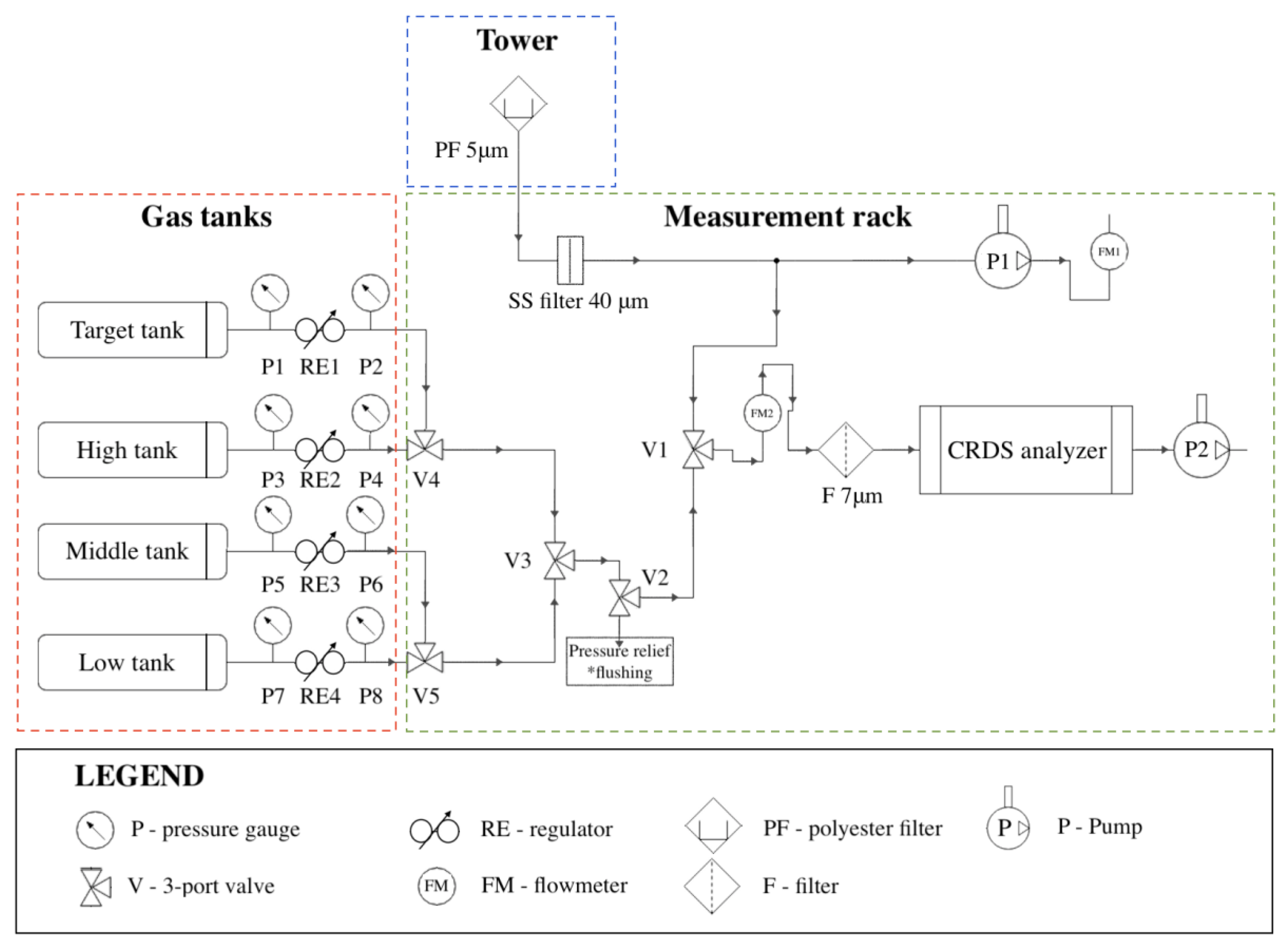
2.2. Instrumentation and Methods

The continuous atmospheric measurements were started in September 2018 and deployed 120 m away from the shoreline of the Yenisei River gulf on the edge of the Dikson settlement. An entire permanent population of the locality comprises ~200 inhabitants. The closest settlements to the measurement site are Vorontsovo (~220 km, population 253 as of 2010) and Karaul (~400 km to the southeast, population 800 as of 2010), with no other settlements closer than 500 km. The proximity of the “DIAMIS” station to the Dikson settlement is related to the harsh environmental conditions and the general lack of infrastructure and power supply that would have prevented deployment and maintenance of the instrumentation at the more remote site. However, the tower sampling at greater height is much less influenced by local contamination events (<3.7% of the observations), and wind distribution analysis ensures the location of the measurement tower is beyond or exclusively rarely receptive to local polluters. During further strict background filters of the raw data, possible pollution signals are removed from the time series.
The observation facility consists of a meteorological mast (Figure 2b), with an air inlet and meteorological sensors installed at the topmost of the tower at 30 m a.g.l (35 m a.s.l.). The trace gas analyzer and the data logger are mounted in a 19′ measurement rack inside a laboratory (Figure 6). Atmospheric air is sucked from the inlet equipped by a 5 μm polyester filter Solberg F-15-50 (Solberg Int. GmbH, Nuremberg, Germany) (PF, Figure 6) through a flexible tubing line SERTOflex 12S (SERTO GmbH, Kassel, Germany) by a membrane pump N815KNDC (KNF Neuberger GmbH, Germany) (P1, Figure 6). A maintained flow rate of 15 L/min in the line is monitored by a flow meter (FM1, Figure 6). The flow inside the sampling tube (internal diameter 8.1 mm) is just turbulent and has a speed of about 4.8 m per second. From the tower, the tubing enters the laboratory room located below. Atmospheric air goes through a 40 μm stainless steel filter, after which the t-connection creates the junction between “high-flow line” and “sample-flow line”. From the high-flow line into the sample-flow line, the air is sucked by a vacuum pump MD 4 NT (Vacuubrand GmbH, Germany) (P2, Figure 6). In the sample line, atmospheric mole fractions of CO2, CH4, and H2O are permanently measured by a cavity ring-down spectroscopy (CRDS) analyzer (Picarro G2301-f, Picarro Inc., Santa Clara, CA, USA) that is regularly calibrated against WMO-traceable reference gases.
Calibration of the CRDS analyzer is performed against pressurized dry air filled at the Max Planck Institute for Biogeochemistry (Jena, Germany) to 6061 Luxfer 40L Aluminium Cylinders (π-certified) (Luxfer Holdings PLC, Manchester, UK) with Rotarex membrane valves of D200 type with PCTFE seat (Rotarex, Luxembourg). In the calibration tanks, concentrations have been traced to the WMO scales X2007 for CO2 [44] and X2004A for CH4 [45]. Dry air mixtures from three calibration tanks (low, middle, and high concentrations) pass through the “low dead volume” pressure regulators (SCOTT MODEL 14 M-14C Nickel-plated brass) (RE1–RE4, Figure 6) that reduce their pressure nearly to the ambient values. The stainless-steel lines from the reference tanks are connected to a system of 3-port solenoid valves SMC VT-307 (SMC Corporation, Japan) (V1–V5, Figure 6) used to select between calibration gases. The calibration cycle automatically starts via an external valve sequencer of the CRDS analyzer every 168 h for 20, 20, and 25 min for Low, Middle, and High tank, respectively. The Target tank is probed every 24 h for 15 min and serves as quality control of the calibration process.
Meteorological observations include wind speed and direction, air temperature, relative humidity, and precipitation amount. A 3-axis sonic anemometer Gill R3-50 (Gill Instruments Ltd., Lymington, UK), measures wind speed and direction and has self-made-wire heating against freezing that starts when air temperature drops below +5 °C. Air temperature and relative humidity are measured by a T/RH sensor Vaisala HMP155 (Vaisala Corp., Helsinki, Finland) and a rain gauge tipping bucket TRM-525M (Texas Electronics Inc., Dallas, TX, USA), which is also equipped with self-made electrical trace heating, is utilized for precipitation records. A linear regression analysis of the recorded meteorological variables at the measurement site against the same time resolution data set recorded at the weather station “The Island of Dikson” (WMO ID: 20647) is shown in Figure 7. Results show high correspondence between data sets for air temperature (r = 0.98, p = 0.0000) (Figure 7a) and wind speed (r = 0.83, p = 0.0000) (Figure 7c), and lower correlation found for relative humidity (r = 0.72, p = 0.0000) (Figure 7b) and wind direction (r = 0.59, p = 0.0000) (Figure 7d).
Trace gas time series are logged by the factory-build software of the CRDS analyzer and an external data logger 9210B Xlite (Sutron Corp., Sterling, VA, USA), which also records meteorological variables. The 9210B Xlite data logger has a communication to the analyzer via RS-232 interface and samples measured variables with a frequency of as high as 5 s, further producing 1-min averages. The internal clocks of the CRDS analyzer secure permanent time synchronization with an SNTP server while the 9210B Xlite receives the analyzer’s PC time every 24 h. To protect the measurement system against possible electrical failures, an uninterruptible power supply APC Smart-UPS X 2200VA SMX2200 (APC Schneider Electric, West Kingston, RI, USA) is capable of buffer power outages of up to ~40 min.
Water impacts the CO2 and CH4 measurements of the CRDS analyzer, causing dilution and pressure broadening. With the constant pressure in the optical cavity, with increasing water vapor pressure, dilution linearly decreases the concentration of trace gas, while pressure broadening is considered as a nonlinear effect [46]. Comparisons with the other observations and for the assimilation of the data series in the atmospheric model products, however, require the dry mixing ratios because wet mixing ratios demonstrate alterations while changing water vapor content. CO2 and CH4 mole fractions are measured by the CRDS analyzer in humid air and include only a first-order water correction function [47], which is not sufficient, as experimentally revealed by [46]. In this study, the relation between H2O concentration and the wet and dry ratios for trace gases in the raw 1-min values reported by the instrument was fitted with a second-order H2O correction function [46,48], using the basic approaches reported elsewhere, e.g., [30,49].
After water correction and implemented calibration coefficients, prior to hourly averaging of the values, invalid data were removed using a set of filters: for bad analyzer status diagnostics, flushing of measurement lines prior and after probing reference air tanks, the timing of calibration and maintenance procedures, and spikes appeared due to contamination from local polluters. The criteria for the spike detection algorithm were based on [32,50] and tuned according to our measurements. The data passed through a set of strict filters for background conditions; in particular, the intra-hour variability of the data records was set as σ(CO2) < 0.2 ppm and σ(CH4) < 4 ppb [32], while the hour-to-hour variability in CO2 was defined as 0.25 ppm [50]. Since large CH4 spikes are frequently matched with CO2 spikes, both corresponding CO2 and CH4 spikes were flagged, even though this could remove some unpolluted CH4 signals. Finally, afternoon data records (1–4 pm local time (LT)) for the daytime mixed layer that is represented throughout a vast area [33] were selected and filtered by wind speed (>2 ms−1). Thus, the implemented strict selecting and timing of the data series allowed us to identify most of those hourly values of well-mixed air in the study area that are representative and not affected by local pollution events.

3. Results and Discussion

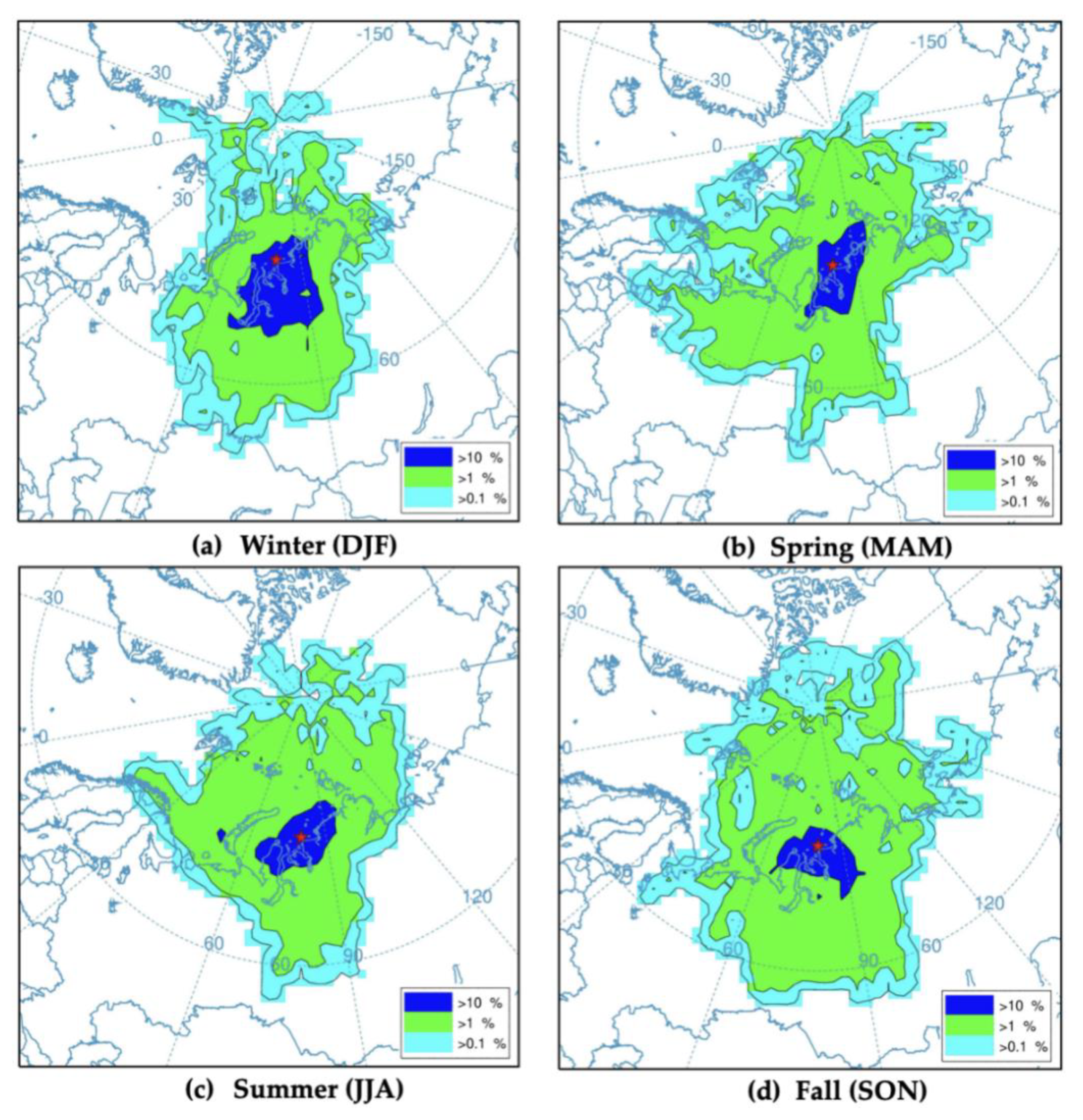
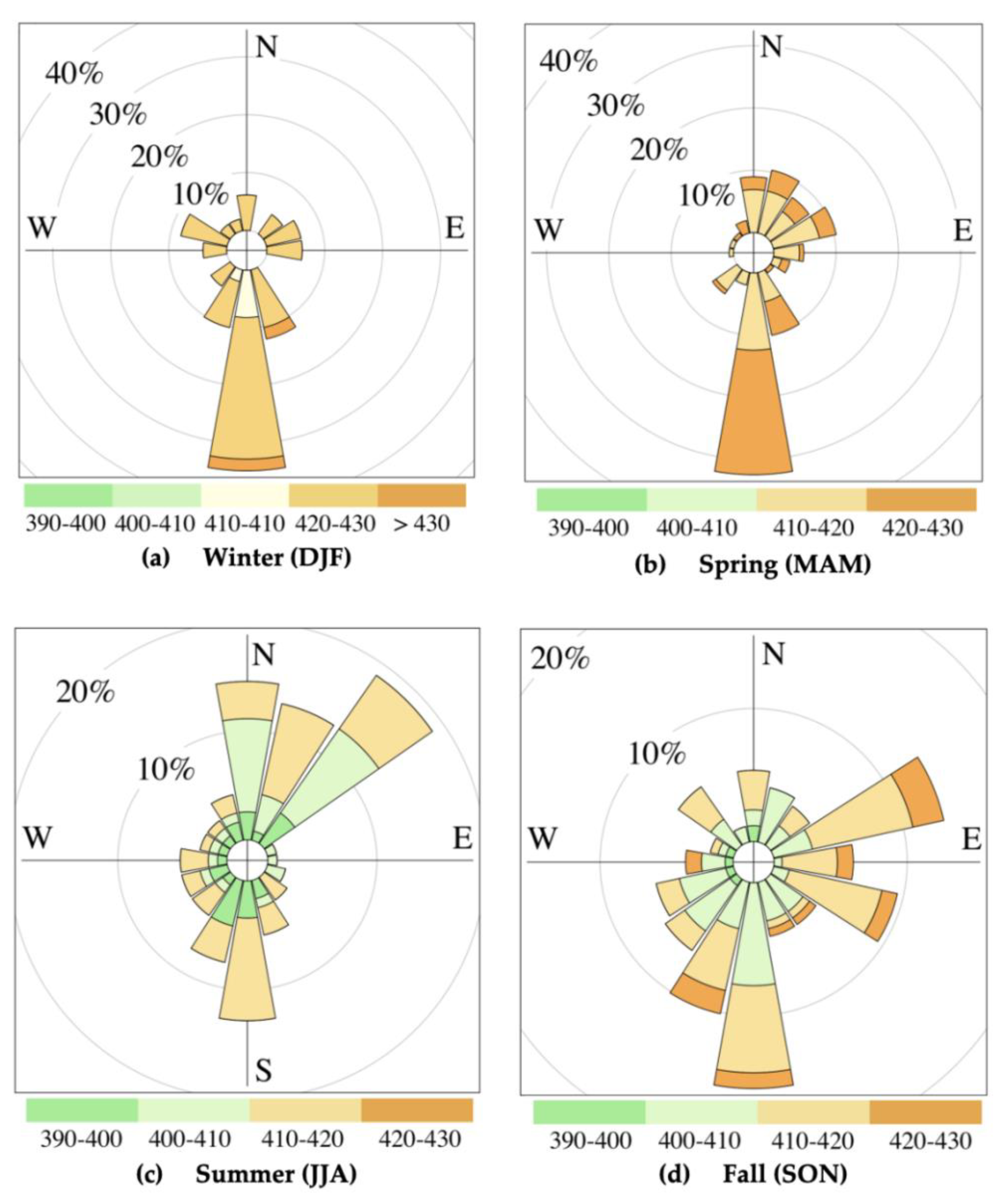
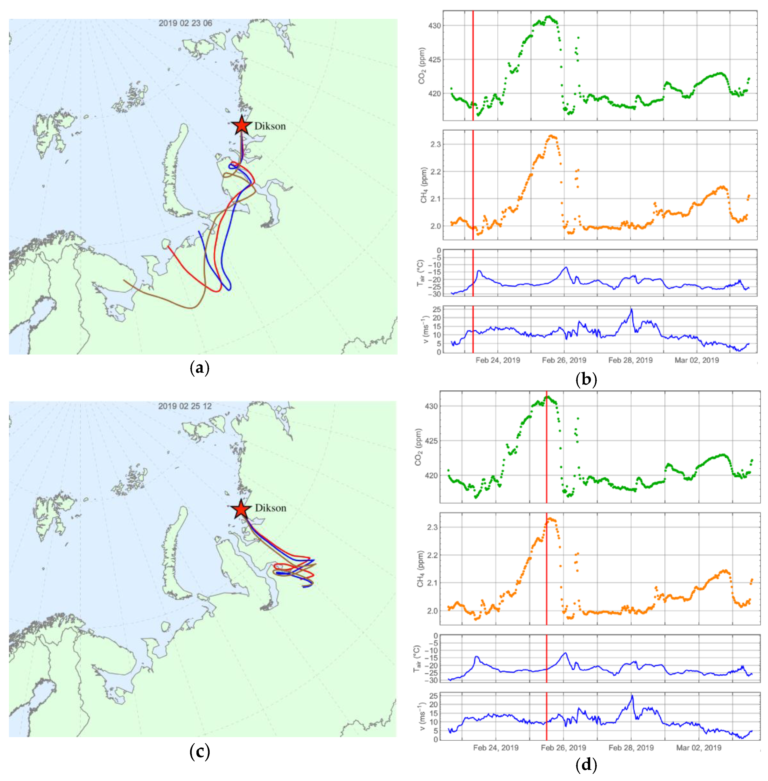
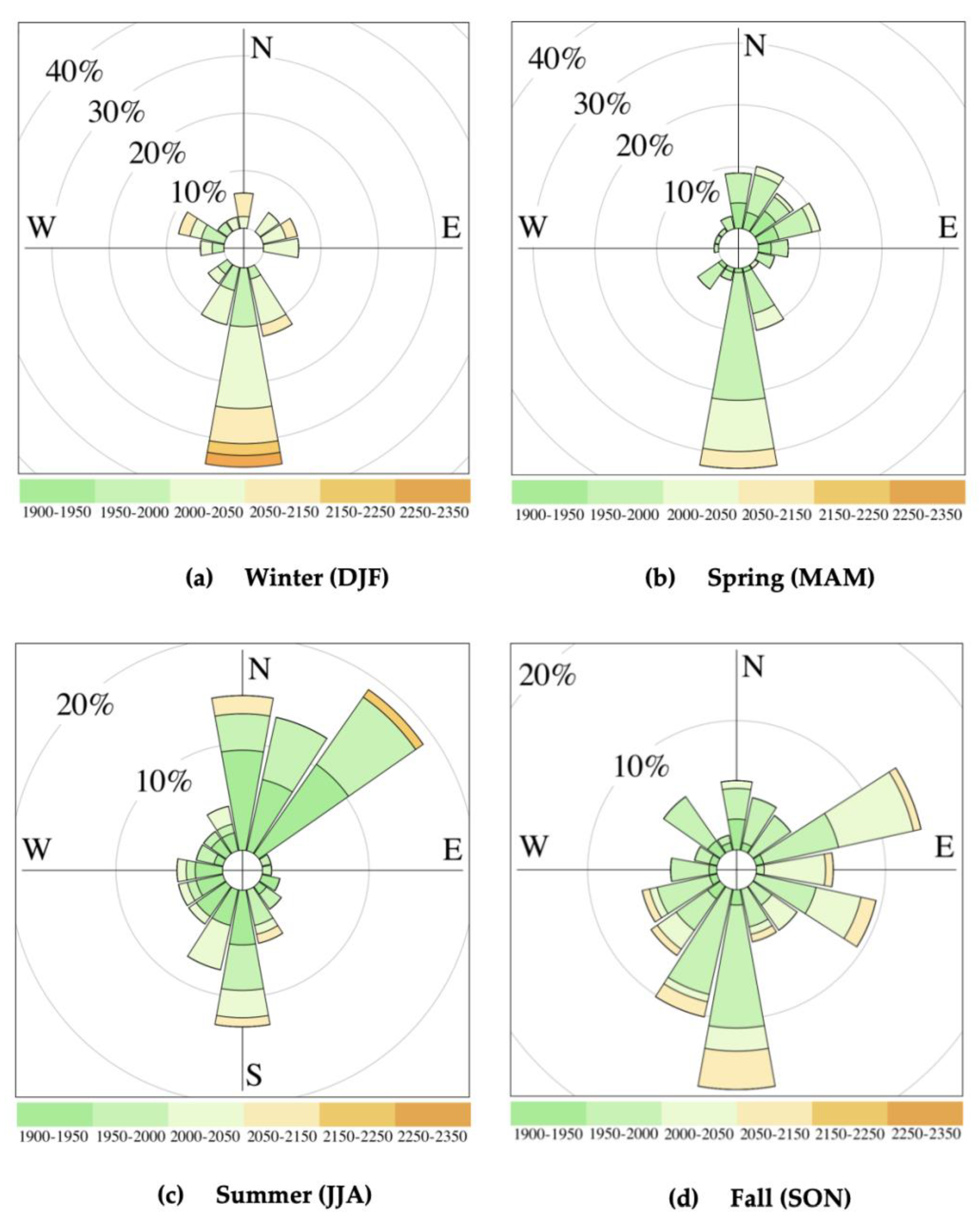
3.1. Seasonal Footprint Analysis for the Measurement Site

For dealing with larger spatial domains, based on the backward trajectory frequency analysis for the period of our observations (September 2018–February 2020), we examined the source regions of air parcels moving into the study area. After calculating, the 5-day backward trajectories were put on a grid over the computational domain, and the number of trajectory intersections over each grid cell was counted and normalized by the total number of trajectories (Figure 8).
These estimates deal with a “footprint” of the measurement site. In general, the footprint shows an obvious correspondence (Figure 8a–c) with longer-term meteorological records (Figure 4a–c), specifically for the major domain of influence (>10% of frequencies observed, dark blue areas in Figure 8). However, we found some deviations between instrumentation records (Figure 4d) and modeled footprint in fall (Figure 8d) that skewed more to the southeast and may reflect large-scale effects over the study domain, e.g., a turn of the seasonal wind drift from summer (north to the northeast) to winter (south to the southwest) dominant directions. Nevertheless, both meteorological observations and footprint analysis imply presumably pristine air coming from the AO in late spring and summer. At the same time, during the frost period, the measurement site may be more receptive to the land surface of northwestern Siberia, capturing carbon signatures both from surrounding tundra ecosystems (e.g., winter methane emissions) [16] and transport of polluted air masses from the Ob-Yamal domain (Figure 8a) that has been a subject of exploration in terms of oil and gas production, as reviewed by [51]. On the other hand, the observed AO influence in summer might be a particular advantage of the site, since the Kara Sea represents a large part of the Siberian Arctic Shelf that is, in contrast to the other shelf environments, characterized by the presence of subsea permafrost and associated gas hydrates buried in the sediments [8]. Continuous trace gas observations might permit early detection of CH4 signals related to destabilizing subsea permafrost and gas hydrate reservoirs.

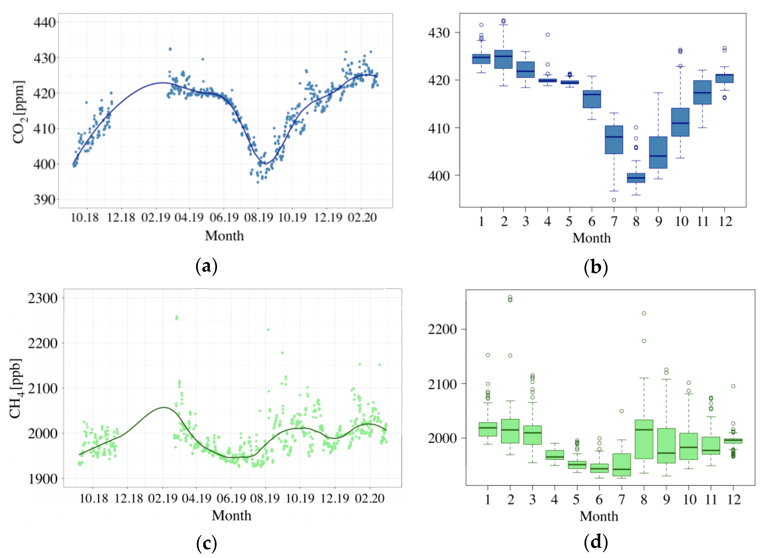
3.2. Temporal Fluctuations of Carbon Dioxide in the Coastal Arctic Atmosphere

Like elsewhere, e.g., [32,52,53,54], the annual amplitude of atmospheric CO2 demonstrates a seasonal pattern (Figure 9a,b) and for the study area could be mostly related to local climate conditions and proximity to the Arctic Ocean.
Particularly, the influence of the AO on the CO2 temporal dynamic applies in the sea ice cover trend, growing up during the frost season and quickly melting in summer. The seasonal pattern shows a sharp decline in CO2 in summer and achieves a maximum in winter (DJF), while a specific second maximum may occur in later winter along with the ice melting and appeared ice-free water areas in the ocean, as reported by [55]. However, during that period, our measurements are predominantly influenced by the continent, achieving as much as 74% of observations, with air masses mostly coming within the relatively narrow tunnel from the south (35%), south-south-east (12%), and to south-south-west (10%) (Figure 10) which might interfere with the oceanic CO2 signal. The contribution of the land surface over the study area is also captured by footprint estimates in winter (Figure 8a).
The influence of the continental domain in winter promotes prominent signals of polluted air masses that may be detected by our measurements, an interesting subject for further case studies. An example of a pollution event is shown in Figure 11 as a relatively long-term atmospheric anomaly observed during a few days in February 2019. To gather insights on possible sources that influenced our observations, with a frequency of 3 h, we computed 5-day backward trajectories using the ARL NOAA HYSPLIT model [41], with the Global Data Assimilation System (GDAS) daily meteorological sets implemented in the computation. For each time, instant three backward trajectories were calculated, starting at 30 m (red), 80 m (blue), and 150 m (brown) a.s.l. (Figure 11a,c). Corresponding records of trace gases, wind speed, and air temperature are summarized in (Figure 11b,d).
The anomaly shows an increscent pronounced growth of CO2 from 418 ppm (Figure 11b) up to the values of >430 ppm (Figure 11d) that is followed by the change in a long-range air mass transport downwind to the measurement site, from the relatively pristine marine area in the Barents Sea (Figure 11a) to the continental domain of the Ob-Yamal area (Figure 11c) that has been extensively explored in terms of oil and gas production as reviewed by [51]. This specific polluted domain is located within the winter footprint of the measurement site (Figure 8a).
A CO2 decline in the atmosphere starts already in March (Figure 9a,b), while low values of air temperature (Figure 3a) and continued continental influence (>60%) observed in our measurements (Figure 10) may illustrate a startup of terrestrial CO2 uptake by vegetation in the more southern regions of northwestern Siberia (Figure 8b). Eventually, an average value of CO2 dry mole fractions observed over the continental domain decreased from 424.1 ± 1.6 ppm recorded in winter to spring rates as of 420.3 ± 0.8 ppm. A further sharp decline of CO2 is observed at the beginning of summer (June) and promoted by positive air temperature (Figure 3a) and snow-melt in the region that is reflected in high (~95%) values of relative humidity (Figure 3b). This transition point may indicate a startup of CO2 photoassimilation by the surrounding tundra ecosystems. On the other hand, the contribution of the AO domain becomes more pronounced in the study area, as the computed footprint in spring shows (Figure 8b).
Unlike the colder (frost) period, summer measurements are more receptive to an influence from the AO that achieves 64% (Figure 10), with air masses mostly traveling from the north to the north-east (46%). The AO influence is clearly illustrated also by the footprint estimate (Figure 8c), showing large-scale effects that agreed with our instrumentation records. The observed oceanic signal shows an average value of CO2 as of 406.4 ± 2.1 ppm, compared to slightly higher rates measured over the continent (407.9 ± 4.7 ppm) but with larger deviations due to stronger alterations of terrestrial carbon signatures over the spatially heterogeneous southern and western areas of the Taimyr Peninsula (Figure 8c). The decline of atmospheric CO2 continues until August, reaching a minimum rate as low as 399.3 ppm (Figure 9a,b), which generally corresponds to earlier reported CO2 summer values across the Arctic latitudes of Northern Eurasia [49,53,54] and might be simultaneously driven by terrestrial signals detected from the continent (36%) and larger contribution (64%) of the AO air masses (Figure 8c and Figure 10).
The growth of CO2 mole fractions in the atmosphere starts being observed in the early to mid-fall, reaching the average rates as of 404.5 and 411.2 ppm by September and October, correspondingly. However, while biological activity presumably occurs over the study area in September that is promoted by positive air temperatures (Figure 3a), the autumnal freeze-in may start by October when the average air temperature drops to slightly negative values, and CO2 emission bursts may be observed due to physical release of carbon dioxide stored in the soil through the frost-induced soil fissures, as was earlier reported by [56]. A continental influence during fall increases up to >60% (Figure 10) with winds mostly blowing from the south to south-south-west (26%) and fewer frequencies observed from east-north-east (13%), showing the CO2 rates as of 411.5 ± 2.4 ppm, compared to lower values detected over the ocean (31%, 407.7 ± 2.6 ppm). In comparison with instrumentation records, the modeled “footprint” during fall (Figure 8d) shows a continental domain, which skewed more to the southeast that, rather than the observations that capture local to regional processes, might reflect large-scale effects over the study domain. Later on, when photosynthetic uptake of CO2 by the vegetation of the area desists, the active soil layer is frozen and microbial activity declines to meager rates compared to summer values [57,58], an autumn-to-winter CO2 build-up is observed, which promotes an increasing trend of carbon dioxide that achieves maximal values by January (424.9 ppm) and February (424.8 ppm) (Figure 9b) and is contributed to mostly by the continent (Figure 8a and Figure 10).

3.3. Temporal Fluctuations of Methane in the Coastal Arctic Atmosphere

Unlike carbon dioxide, a pattern of atmospheric methane shows a flatter baseline with fewer variations throughout the year (Figure 9c,d), but a seasonal trend with a maximum in colder seasons and a pronounced minimum during mid-summer may be observed, as earlier reported by [31,32]. In winter (polar night), photochemical reactions with atmospheric OH radicals, serving as methane sink, do not occur, as noted by [59] and generally presumed to be a particular factor that applies in more southern regions. For the study area in the high latitudes, the seasonally varying sources and atmospheric transport of CH4 may be of a larger influence. Similar to CO2, the winter pattern of atmospheric methane is mostly contributed by the land surface (Figure 8a and Figure 12) with an average value as of 2020.5 ± 17.4 ppb, which is nearly the same as observed for the less frequent oceanic CH4 signal (2019.8 ± 18.8 ppb). Given the absence of biogenic methane signals in the area, except for CH4 winter emissions in earlier periods [16], and local methane sources in the neighbored Yamal and Gydan Peninsula as reported by [51], we may consider the man-caused CH4 signatures as prevailing for study area during the frost period. An example of the winter contamination anomaly of CH4 that we reported in the previous Section 3.2. (Figure 11), and showing atmospheric methane increased from 2000 up to as high as >2300 ppb along with air masses coming from the relatively polluted area, may also confirm this speculation. As mentioned above, the modeled winter footprint of the study area captures this polluted domain (Figure 8a).
During summer, the seasonal composition of atmospheric methane demonstrates an increased influence (up to 64%) of comparatively pristine air masses from the Arctic Ocean (Figure 12) and showing average CH4 rates as low as 1962.6 ± 8.8 ppb. The relatively small deviation of the CH4 values may presume relatively constant and similar methane signatures over the AO, compared to the observed continental values that are slightly higher (1970.5 ± 22.6 ppb) but show the much stronger fluctuation of terrestrial CH4 signals representing southern and western parts of the Taimyr Peninsula as summer footprint shows (Figure 8c). This corresponds well with findings for the western part of the Yamal Peninsula achieved by [60], who reported the large deviations of near-surface CH4 concentrations in the range as high as 1600–5000 ppb for swampy polygonal tundra and wetlands and much lower values as of 90–300 ppb observed in the drained tundra and sandy fields.
The maximal air temperature recorded in July and August (Figure 3a) warmed the seasonally thawed soil layer and, along with the observed CH4 minimum (Figure 9c,d), might have triggered the large CH4 enhancements presumably related to strong regional sources. In contrast to minimal values of CO2 recorded in August, a CH4 minimum is observed a month earlier (July) as of 1938.6 ppb. In August, the precipitation amount (Figure 3d) demonstrates the highest annual records that might serve as a reason for the physical release of methane stored in the soil pores by rainwater and most likely contributing to the enhanced CH4 levels in the atmosphere. A water table depth might also be considered as an indirect factor that controlled the abundance of vascular plants influencing carbon turnover through root exudates and plant-mediated release of methane, as reported by [61].
In fall (SON), both instrumental observations (Figure 12) and footprint estimates (Figure 8c) suggest the growing influence of continental CH4 signatures, with air masses mostly coming from the south to south-south-west (26%) and fewer cases recorded from east-north-east (13%) (Figure 12). The average methane mole fractions observed from the continent show essentially higher values as of 1999.8 ± 13.2 ppb, compared to rates recorded over the ocean (1961.9 ± 11.2 ppb). For the major continental directions that contributed to our measurements in fall, the higher CH4 values (2001.6 ppb) were recorded for southern directions—areas of the southern domain of the western Taimyr Peninsula and further central Siberia—while lower rates (1993.4 ppb) observed for the east-north-east (Figure 12), representing relatively pristine northern and more eastern areas of the Taimyr Peninsula. A temporal pattern shows a general increasing trend of atmospheric methane that may be observed until January when it achieves a winter maximum as of 2021.3 ppb (Figure 9c,d). As reported by [62], during earlier colder months, a large part of the active soil layer may stay unfrozen for an extended period of time while air temperatures fluctuate around 0 °C, representing the so-called “zero curtain” period that is mostly related to CH4 emissions during the colder season and may contribute up to 50% of the annual methane flux [16]. The large CH4 enhancements during fall might be partly attributed to soil freezing toward the end of the “zero curtain” in November when air temperature sharply drops to average negative values (Figure 3a), but on the other hand, an influence of CH4 sources from the more southern Siberian regions (Figure 8c) might also be traced.

4. Conclusions

The recently deployed measurement station for continuous observations of atmospheric carbon dioxide (CO2) and methane (CH4) dry mole fractions in the western Taimyr Peninsula at the gulf of the Yenisei River—one of the major Arctic River catchments in Siberia and Northern Eurasia—fills a significant gap in the atmospheric trace gas observations over the Arctic belt of central Siberian domain. Here, we summarized the scientific rationale of the new site, described technical details of the instrumental setup and applied methodology, analyzed the local environments, and examined the seasonal footprint.
The seasonal footprint estimates for the measurement site and meteorological records imply presumably pristine air coming from the Arctic Ocean in late spring and summer, while observations during the frost period may be more receptive to the continental part of northwestern Siberia, capturing biogenic sources from surrounding ecosystems and polluted air anomalies, hence characterizing carbon signatures over the two predominant domains—marine shelf areas of the Kara Sea (AO) and the land surface.
Despite the relatively short-term record (September 2018–February 2020), the first results of the atmospheric observations illustrate a seasonal pattern of CO2 and CH4 for the daytime mixed layer of the Arctic atmosphere that is represented throughout a large area (~500–1000 km) of the Siberian Arctic domain. Further data series will provide insights into seasonal patterns, including intra- and inter-annual fluctuations and long-term trends that are not considered here.
Based on the footprint analysis and angular distribution of atmospheric dry mole fractions CO2 and CH4 across the prevailing wind directions, we have shown a seasonal contribution of different spatial domains to the recorded trace gas fluctuations, which can serve as a preliminary overview of carbon signatures over the studied Arctic domain in central Siberia for further research.

Author Contributions

Conceptualization, A.P. (Alexey Panov), A.P. (Anatoly Prokushkin), and M.H.; methodology, A.P. (Alexey Panov), K.R.K. and M.K.; software, A.P. (Alexey Panov), A.U. and M.K.; validation, M.K., A.P. (Alexey Panov), and A.P. (Anatoly Prokushkin); formal analysis, A.P. (Alexey Panov) and M.K.; investigation, A.P. (Alexey Panov) and A.P. (Anatoly Prokushkin); resources, M.B.; data curation, A.P. (Alexey Panov); writing—original draft preparation, A.P. (Alexey Panov); writing—review and editing, A.P. (Alexey Panov) and A.P. (Anatoly Prokushkin); visualization, A.P. (Alexey Panov); supervision, A.P. (Alexey Panov) and M.H.; funding acquisition, A.P. (Alexey Panov), A.P. (Anatoly Prokushkin), and M.H. All authors have read and agreed to the published version of the manuscript.

Funding

This research was funded by the Russian Foundation for Basic Research, Krasnoyarsk Territory, and Krasnoyarsk Regional Fund of Science, project #20-45-242908, RFBR under the research project #18-05-60203, and by the Max Planck Society (Germany). The tasks of M.H. were supported by the Russian Science Foundation, project #21-17-00163, and Q-ARCTIC ERC Synergy project.

Institutional Review Board Statement

Not applicable.

Informed Consent Statement

Not applicable.

Data Availability Statement

The used atmospheric observational data are available at https://data.mendeley.com/datasets/2vvgs2rw9c/1 (doi:10.17632/2vvgs2rw9c.1) (accessed on 4 June 2021). Publicly available meteorological archived datasets analyzed in this study can be found at https://rp5.ru (accessed on 17 May 2021). The publicly available HYbrid Single-Particle Lagrangian Integrated Trajectory (HYSPLIT) model can be found at https://www.ready.noaa.gov/HYSPLIT.php (accessed on 19 June 2021) and run either online or offline.

Acknowledgments

The authors would like to thank Igor Kornienko (the Big Arctic Reserve, Dikson) for his permanent support of the measurements on the site. We also acknowledge the work of Alexander Tsukanov, Sergey Titov, Vyacheslav Zyrianov (SIF SB RAS, Krasnoyarsk), and Waldemar Ziegler (MPI-BGC, Germany) for their help with the installation and maintenance of the tower, technical suggestions, and improvements.

Conflicts of Interest

The authors declare no conflict of interest.

References

  1. IPCC: The Ocean and Cryosphere in a Changing Climate. Available online: https://www.ipcc.ch/srocc/home (accessed on 1 June 2021).
  2. Arctic Report Card: Update for 2020. Available online: https://arctic.noaa.gov/Report-Card/Report-Card-2020 (accessed on 1 June 2021).
  3. Fraser, R.H.; Lantz, T.C.; Olthof, I.; Kokelj, S.V.; Sims, R.A. Warming-Induced Shrub Expansion and Lichen Decline in the Western Canadian Arctic. Ecosystems 2014, 17, 1151–1168. [Google Scholar] [CrossRef]
  4. Serreze, M.C.; Walsh, J.E.; Iii, F.S.C.; Osterkamp, T.; Dyurgerov, M.; Romanovsky, V.; Oechel, W.; Morison, J.; Zhang, T.; Barry, R.G. Observational Evidence of Recent Change in the Northern High-Latitude Environment. Clim. Chang. 2000, 46, 159–207. [Google Scholar] [CrossRef]
  5. Bhatt, U.S.; Walker, D.A.; Raynolds, M.K.; Comiso, J.C.; Epstein, H.E.; Jia, G.; Gens, R.; Pinzon, J.E.; Tucker, C.J.; Tweedie, C.E.; et al. Circumpolar Arctic Tundra Vegetation Change Is Linked to Sea Ice Decline. Earth Interact. 2010, 14, 1–20. [Google Scholar] [CrossRef] [Green Version]
  6. Hinzman, L.D.; Deal, C.J.; McGuire, A.D.; Mernild, S.H.; Polyakov, I.V.; Walsh, J.E. Trajectory of the Arctic as an integrated system. Ecol. Appl. 2013, 23, 1837–1868. [Google Scholar] [CrossRef] [PubMed]
  7. Park, T.; Ganguly, S.; Tømmervik, H.; Euskirchen, E.S.; Høgda, K.-A.; Karlsen, S.R.; Brovkin, V.; Nemani, R.R.; Myneni, R. Changes in growing season duration and productivity of northern vegetation inferred from long-term remote sensing data. Environ. Res. Lett. 2016, 11, 084001. [Google Scholar] [CrossRef]
  8. Romanovskii, N.N.; Hubberten, H.-W.; Gavrilov, A.V.; Eliseeva, A.A.; Tipenko, G. Offshore permafrost and gas hydrate stability zone on the shelf of East Siberian Seas. Geo-Mar. Lett. 2005, 25, 167–182. [Google Scholar] [CrossRef] [Green Version]
  9. McGuire, A.D.; Anderson, L.G.; Christensen, T.R.; Dallimore, S.; Guo, L.; Hayes, D.J.; Heimann, M.; Lorenson, T.D.; Macdonald, R.; Roulet, N. Sensitivity of the carbon cycle in the Arctic to climate change. Ecol. Monogr. 2009, 79, 523–555. [Google Scholar] [CrossRef] [Green Version]
  10. Hayes, D.J.; Kicklighter, D.W.; McGuire, A.D.; Chen, M.; Zhuang, Q.; Yuan, F.; Melillo, J.M.; Wullschleger, S.D. The impacts of recent permafrost thaw on land–atmosphere greenhouse gas exchange. Environ. Res. Lett. 2014, 9, 045005. [Google Scholar] [CrossRef] [Green Version]
  11. Schuur, E.A.G.; McGuire, A.D.; Schadel, C.; Grosse, G.; Harden, J.W.; Hayes, D.J.; Hugelius, G.; Koven, C.; Kuhry, P.; Lawrence, D.; et al. Climate change and the permafrost carbon feedback. Nature 2015, 520, 171–179. [Google Scholar] [CrossRef]
  12. Angert, A.; Biraud, S.; Bonfils, C.; Henning, C.C.; Buermann, W.; Pinzon, J.; Tucker, C.J.; Fung, I. Drier summers cancel out the CO2 uptake enhancement induced by warmer springs. Proc. Natl. Acad. Sci. USA 2005, 102, 10823–10827. [Google Scholar] [CrossRef] [Green Version]
  13. Oechel, W.C.; Cowles, S.; Grulke, N.; Hastings, S.J.; Lawrence, B.; Prudhomme, T.; Riechers, G.; Strain, B.; Tissue, D.; Vourlitis, G. Transient nature of CO2 fertilization in Arctic tundra. Nature 1994, 371, 500–503. [Google Scholar] [CrossRef]
  14. Goetz, S.J.; Bunn, A.; Fiske, G.J.; Houghton, R.A. Satellite-observed photosynthetic trends across boreal North America associated with climate and fire disturbance. Proc. Natl. Acad. Sci. USA 2005, 102, 13521–13525. [Google Scholar] [CrossRef] [PubMed] [Green Version]
  15. Webb, E.; Schuur, E.A.G.; Natali, S.M.; Oken, K.L.; Bracho, R.; Krapek, J.P.; Risk, D.; Nickerson, N.R. Increased wintertime CO2 loss as a result of sustained tundra warming. J. Geophys. Res. Biogeosci. 2016, 121, 249–265. [Google Scholar] [CrossRef] [Green Version]
  16. Zona, D.; Gioli, B.; Commane, R.; Lindaas, J.; Wofsy, S.C.; Miller, C.E.; Dinardo, S.J.; Dengel, S.; Sweeney, C.; Karion, A.; et al. Cold season emissions dominate the Arctic tundra methane budget. Proc. Natl. Acad. Sci. USA 2016, 113, 40–45. [Google Scholar] [CrossRef] [Green Version]
  17. Dlugokencky, E.J.; Bruhwiler, L.; White, J.W.C.; Emmons, L.K.; Novelli, P.C.; Montzka, S.; Masarie, K.A.; Lang, P.M.; Crotwell, A.M.; Miller, J.; et al. Observational constraints on recent increases in the atmospheric CH4 burden. Geophys. Res. Lett. 2009, 36, 18803. [Google Scholar] [CrossRef] [Green Version]
  18. O’Connor, F.M.; Boucher, O.; Gedney, N.; Jones, C.D.; Folberth, G.; Coppell, R.; Friedlingstein, P.; Collins, W.J.; Chappellaz, J.; Ridley, J.; et al. Possible role of wetlands, permafrost, and methane hydrates in the methane cycle under future climate change: A review. Rev. Geophys. 2010, 48, 4005. [Google Scholar] [CrossRef]
  19. Nauta, A.L.; Heijmans, M.M.P.D.; Blok, D.; Limpens, J.; Elberling, B.; Gallagher, A.; Li, B.; Petrov, R.E.; Maximov, T.C.; Van Huissteden, J.; et al. Permafrost collapse after shrub removal shifts tundra ecosystem to a methane source. Nat. Clim. Chang. 2015, 5, 67–70. [Google Scholar] [CrossRef]
  20. Fisher, J.P.; Estop-Aragonés, C.; Thierry, A.; Charman, D.; Wolfe, S.; Hartley, I.P.; Murton, J.B.; Williams, M.; Phoenix, G.K. The influence of vegetation and soil characteristics on active-layer thickness of permafrost soils in boreal forest. Glob. Chang. Biol. 2016, 22, 3127–3140. [Google Scholar] [CrossRef]
  21. Berchet, A.; Bousquet, P.; Pison, I.; Locatelli, R.; Chevallier, F.; Paris, J.-D.; Dlugokencky, E.J.; Laurila, T.; Hatakka, J.; Viisanen, Y.; et al. Atmospheric constraints on the methane emissions from the East Siberian Shelf. Atmos. Chem. Phys. Discuss. 2016, 16, 4147–4157. [Google Scholar] [CrossRef] [Green Version]
  22. Sweeney, C.; Dlugokencky, E.; Miller, C.E.; Wofsy, S.; Karion, A.; Dinardo, S.; Chang, R.Y.; Miller, J.; Bruhwiler, L.; Crotwell, A.M.; et al. No significant increase in long-term CH4emissions on North Slope of Alaska despite significant increase in air temperature. Geophys. Res. Lett. 2016, 43, 6604–6611. [Google Scholar] [CrossRef] [Green Version]
  23. Neumann, R.B.; Moorberg, C.J.; Lundquist, J.D.; Turner, J.C.; Waldrop, M.P.; McFarland, J.W.; Euskirchen, E.S.; Edgar, C.W.; Turetsky, M.R. Warming Effects of Spring Rainfall Increase Methane Emissions from Thawing Permafrost. Geophys. Res. Lett. 2019, 46, 1393–1401. [Google Scholar] [CrossRef]
  24. Douglas, T.A.; Turetsky, M.R.; Koven, C.D. Increased rainfall stimulates permafrost thaw across a variety of Interior Alaskan boreal ecosystems. NPJ Clim. Atmos. Sci. 2020, 3, 28. [Google Scholar] [CrossRef]
  25. Dmitrenko, I.A.; Kirillov, S.A.; Tremblay, L.B.; Kassens, H.; Anisimov, O.; Lavrov, S.A.; Razumov, S.O.; Grigoriev, M.N. Recent changes in shelf hydrography in the Siberian Arctic: Potential for subsea permafrost instability. J. Geophys. Res. Space Phys. 2011, 116, 10027. [Google Scholar] [CrossRef]
  26. Janout, M.; Hoelemann, J.; Juhls, B.; Krumpen, T.; Rabe, B.; Bauch, D.; Wegner, C.; Kassens, H.; Timokhov, L. Episodic warming of near-bottom waters under the Arctic sea ice on the central Laptev Sea shelf. Geophys. Res. Lett. 2016, 43, 264–272. [Google Scholar] [CrossRef] [Green Version]
  27. Zhang, J.; Rothrock, D.A.; Steele, M. Warming of the Arctic Ocean by a strengthened Atlantic Inflow: Model results. Geophys. Res. Lett. 1998, 25, 1745–1748. [Google Scholar] [CrossRef]
  28. Ruppel, C.D.; Kessler, J.D. The interaction of climate change and methane hydrates. Rev. Geophys. 2017, 55, 126–168. [Google Scholar] [CrossRef]
  29. Sasakawa, M.; Shimoyama, K.; Machida, T.; Tsuda, N.; Suto, H.; Arshinov, M.; Davydov, D.; Fofonov, A.; Krasnov, O.; Saeki, T.; et al. Continuous measurements of methane from a tower network over Siberia. Tellus B Chem. Phys. Meteorol. 2010, 62, 403–416. [Google Scholar] [CrossRef]
  30. Winderlich, J.; Chen, H.; Gerbig, C.; Seifert, T.; Kolle, O.; Lavric, J.V.; Kaiser, C.; Hofer, A.; Heimann, M. Continuous low-maintenance CO2/CH4/H2O measurements at the Zotino Tall Tower Observatory (ZOTTO) in Central Siberia. Atmos. Meas. Tech. 2010, 3, 1113–1128. [Google Scholar] [CrossRef] [Green Version]
  31. Heimann, M.; Schulze, E.-D.; Winderlich, J.; Andreae, M.O.; Chi, X.; Gerbig, C.; Kolle, O.; Kubler, K.; Lavric, J.; Mikhailov, E.; et al. The Zotino Tall Tower Observatory (ZOTTO): Quantifying Large Biogeochemical Changes in Central Siberia. Nova Acta Leopold. 2014, 117, 51–64. [Google Scholar]
  32. Reum, F.; Göckede, M.; Lavric, J.V.; Kolle, O.; Zimov, S.; Zimov, N.; Pallandt, M.; Heimann, M. Accurate measurements of atmospheric carbon dioxide and methane mole fractions at the Siberian coastal site Ambarchik. Atmos. Meas. Tech. 2019, 12, 5717–5740. [Google Scholar] [CrossRef] [Green Version]
  33. Karion, A.; Sweeney, C.; Miller, J.B.; Andrews, A.E.; Commane, R.; Dinardo, S.; Henderson, J.M.; Lindaas, J.; Lin, J.C.; Luus, K.A.; et al. Investigating Alaskan methane and carbon dioxide fluxes using measurements from the CARVE tower. Atmos. Chem. Phys. Discuss. 2016, 16, 5383–5398. [Google Scholar] [CrossRef] [Green Version]
  34. Tuovinen, J.-P.; Aurela, M.; Hatakka, J.; Räsänen, A.; Virtanen, T.; Mikola, J.; Ivakhov, V.; Kondratyev, V.; Laurila, T. Interpreting eddy covariance data from heterogeneous Siberian tundra: Land-cover-specific methane fluxes and spatial representativeness. Biogeosciences 2019, 16, 255–274. [Google Scholar] [CrossRef] [Green Version]
  35. Virkkala, A.-M.; Virtanen, T.; Lehtonen, A.; Rinne, J.; Luoto, M. The current state of CO2 flux chamber studies in the Arctic tundra. Prog. Phys. Geogr. Earth Environ. 2017, 42, 162–184. [Google Scholar] [CrossRef] [Green Version]
  36. Sachs, T.; Giebels, M.; Boike, J.; Kutzbach, L. Environmental controls on CH4 emission from polygonal tundra on the microsite scale in the Lena river delta, Siberia. Glob. Chang. Biol. 2010, 16, 3096–3110. [Google Scholar] [CrossRef]
  37. Holmes, R.M.; McClelland, J.W.; Peterson, B.J.; Tank, S.E.; Bulygina, E.; Eglinton, T.I.; Gordeev, V.V.; Gurtovaya, T.Y.; Raymond, P.A.; Repeta, D.J.; et al. Seasonal and Annual Fluxes of Nutrients and Organic Matter from Large Rivers to the Arctic Ocean and Surrounding Seas. Estuaries Coasts 2012, 35, 369–382. [Google Scholar] [CrossRef]
  38. Treshnikov, A.F. Atlas of the Arctic. In Main Directorate of Geodesy and Cartography under the Council of Ministers of the USSR; USSR: Moscow, Russia, 1985; p. 204. (In Russian) [Google Scholar]
  39. McKnight, T.L.; Hess, D. Climate Zones and Types: The Köppen System, Physical Geography: A Landscape Appreciation; Prentice Hall: Hoboken, NJ, USA, 2000; pp. 235–237. [Google Scholar]
  40. Staalesen, A. Northernmost Russian town is epicenter in unprecedented Arctic heatwave. Barents Obs. 2020, 9, 1–4. [Google Scholar]
  41. Stein, A.F.; Draxler, R.R.; Rolph, G.D.; Stunder, B.J.B.; Cohen, M.D.; Ngan, F. NOAA’s HYSPLIT Atmospheric Transport and Dispersion Modeling System. Bull. Am. Meteorol. Soc. 2015, 96, 2059–2077. [Google Scholar] [CrossRef]
  42. Chuvilin, E.; Ekimova, V.; Davletshina, D.; Sokolova, N.; Bukhanov, B. Evidence of Gas Emissions from Permafrost in the Russian Arctic. Geoscience 2020, 10, 383. [Google Scholar] [CrossRef]
  43. Walker, D.A.; Raynolds, M.K.; Daniëls, F.J.; Einarsson, E.; Elvebakk, A.; Gould, W.A.; Katenin, A.E.; Kholod, S.S.; Markon, C.J.; Melnikov, E.S.; et al. The Circumpolar Arctic vegetation map. J. Veg. Sci. 2005, 16, 267–282. [Google Scholar] [CrossRef]
  44. Tulp, I.; Bruinzeel, L.; Jukema, J.; Stepanova, O. Breeding Waders at Medusa Bay, Western Taimyr, in 1996; WIWO Report 57; WIWO: Zeist, The Netherlands, 1997; Volume 57, pp. 7–8. [Google Scholar]
  45. Zhao, C.L.; Tans, P.P. Estimating uncertainty of the WMO mole fraction scale for carbon dioxide in air. J. Geophys. Res. Space Phys. 2006, 111. [Google Scholar] [CrossRef]
  46. Dlugokencky, E.J.; Myers, R.C.; Lang, P.M.; Masarie, K.A.; Crotwell, A.M.; Thoning, K.W.; Hall, B.D.; Elkins, J.W.; Steele, L.P. Conversion of NOAA atmospheric dry air CH4mole fractions to a gravimetrically prepared standard scale. J. Geophys. Res. Space Phys. 2005, 110, 18306. [Google Scholar] [CrossRef]
  47. Chen, H.; Winderlich, J.; Gerbig, C.; Hoefer, A.; Rella, C.W.; Crosson, E.R.; Van Pelt, A.D.; Steinbach, J.H.; Kolle, O.; Beck, V.; et al. High-accuracy continuous airborne measurements of greenhouse gases (CO2 and CH4) using the cavity ring-down spectroscopy (CRDS) technique. Atmos. Meas. Tech. 2010, 3, 375–386. [Google Scholar] [CrossRef] [Green Version]
  48. Crosson, E.R. A cavity ring-down analyzer for measuring atmospheric levels of methane, carbon dioxide, and water vapor. Appl. Phys. B 2008, 92, 403–408. [Google Scholar] [CrossRef]
  49. Rella, C.W.; Chen, H.; Andrews, A.E.; Filges, A.; Gerbig, C.; Hatakka, J.; Karion, A.; Miles, N.; Richardson, S.J.; Steinbacher, M.; et al. High accuracy measurements of dry mole fractions of carbon dioxide and methane in humid air. Atmos. Meas. Tech. 2013, 6, 837–860. [Google Scholar] [CrossRef] [Green Version]
  50. Reum, F.; Gerbig, C.; Lavric, J.V.; Rella, C.W.; Göckede, M. Correcting atmospheric CO2 and CH4 mole fractions obtained with Picarro analyzers for sensitivity of cavity pressure to water vapor. Atmos. Meas. Tech. 2019, 12, 1013–1027. [Google Scholar] [CrossRef] [Green Version]
  51. Thoning, K.W.; Tans, P.P.; Komhyr, W.D. Atmospheric carbon dioxide at Mauna Loa Observatory: 2. Analysis of the NOAA GMCC data, 1974–1985. J. Geophys. Res. Space Phys. 1989, 94, 8549–8565. [Google Scholar] [CrossRef]
  52. Belikov, D.; Arshinov, M.; Belan, B.; Davydov, D.; Fofonov, A.; Sasakawa, M.; Machida, T. Analysis of the Diurnal, Weekly, and Seasonal Cycles and Annual Trends in Atmospheric CO2 and CH4 at Tower Network in Siberia from 2005 to 2016. Atmosphere 2019, 10, 689. [Google Scholar] [CrossRef] [Green Version]
  53. Ivakhov, V.M.; Paramonova, N.N.; Privalov, V.I.; Zinchenko, A.V.; Loskutova, M.A.; Makshtas, A.P.; Kustov, V.Y.; Laurila, T.; Aurela, M.; Asmi, E. Atmospheric Concentration of Carbon Dioxide at Tiksi and Cape Baranov Stations in 2010–2017. Russ. Meteorol. Hydrol. 2019, 44, 291–299. [Google Scholar] [CrossRef]
  54. Antonov, K.L.; Poddubny, V.; Markelov, Y.I.; Buevich, A.G.; Medvedev, A.N. Dynamics of surface carbon dioxide and methane concentrations on the Arctic Belyy Island in 2015–2017 summertime. In Proceedings of the 24th International Symposium on Atmospheric and Ocean Optics: Atmospheric Physics, Tomsk, Russia, 2–5 July 2018; Volume 10833. [Google Scholar] [CrossRef]
  55. Alekseev, G.V.; Nagurnyi, A.P. Influence of sea ice cover on carbon dioxide concentration in the Arctic atmosphere in the winter period. Dokl. Earth Sci. 2005, 401, 486–489. [Google Scholar]
  56. Pirk, N.; Santos, T.; Gustafson, C.; Johansson, A.J.; Tufvesson, F.; Parmentier, F.W.; Mastepanov, M.; Christensen, T. Methane emission bursts from permafrost environments during autumn freeze-in: New insights from ground-penetrating radar. Geophys. Res. Lett. 2015, 42, 6732–6738. [Google Scholar] [CrossRef]
  57. Björkman, M.P.; Morgner, E.; Cooper, E.J.; Elberling, B.; Klemedtsson, L.; Björk, R.G. Winter carbon dioxide effluxes from Arctic ecosystems: An overview and comparison of methodologies. Glob. Biogeochem. Cycles 2010, 24, 3010. [Google Scholar] [CrossRef]
  58. Drotz, S.H.; Sparrman, T.; Nilsson, M.B.; Schleucher, J.; Oquist, M.G. Both catabolic and anabolic heterotrophic microbial activity proceed in frozen soils. Proc. Natl. Acad. Sci. USA 2010, 107, 21046–21051. [Google Scholar] [CrossRef] [Green Version]
  59. Montzka, S.A.; Krol, M.; Dlugokencky, E.; Hall, B.; Jockel, P.; Lelieveld, J. Small Interannual Variability of Global Atmospheric Hydroxyl. Science 2011, 331, 67–69. [Google Scholar] [CrossRef] [PubMed] [Green Version]
  60. Vasiliev, A.A.; Melnikov, V.P.; Semenov, P.B.; Oblogov, G.E.; Streletskaya, I.D. Methane Concentration and Emission in Dominant Landscapes of Typical Tundra of Western Yamal. Dokl. Earth Sci. 2019, 485, 284–287. [Google Scholar] [CrossRef]
  61. Ström, L.; Mastepanov, M.; Christensen, T. Species-specific Effects of Vascular Plants on Carbon Turnover and Methane Emissions from Wetlands. Biogeochemistry 2005, 75, 65–82. [Google Scholar] [CrossRef]
  62. Hinkel, K.; Paetzold, F.; Nelson, F.; Bockheim, J. Patterns of soil temperature and moisture in the active layer and upper permafrost at Barrow, Alaska: 1993–1999. Glob. Planet. Chang. 2001, 29, 293–309. [Google Scholar] [CrossRef]
Figure 1. Network of stations continuously measuring atmospheric CO2 and CH4 mole fractions across the Arctic domain of Siberia.
Atmosphere 12 00876 g001
Figure 2. Location of the measurement site at the Gulf of the Yenisei River in the western Taimyr Peninsula (a) and a meteorological tower for continuous atmospheric observations (b).
Atmosphere 12 00876 g002
Figure 3. Variability of the monthly mean air temperature (a), relative humidity (b), wind speed (c), and daily precipitation amounts (d) for the period of observations at the measurement station “DIAMIS”. On each box, the central line shows the median. The bares represent the lower “hinge” and the upper “hinge” and the extremes of the upper and lower whiskers. Dots indicate outliers.
Atmosphere 12 00876 g003
Figure 4. Mean wind distribution throughout the year recorded at the weather station “The Island of Dikson” (WMO ID: 20674) for 15 years of observations (2005–2020): frequency of counts (%) and speed (m/s).
Atmosphere 12 00876 g004
Figure 5. Classification and mapping of the land cover classes for the study area based on the Landsat 8 OLI (18 July 2017) and the Terra Norte RLC vegetation map.
Atmosphere 12 00876 g005
Figure 6. Air flow diagram of the instrumental setup at the measurement site.
Atmosphere 12 00876 g006
Figure 7. Linear regression analysis for the two data sets of meteorological records at the measurement station “DIAMIS” and the weather station “The Island of Dikson” (WMO ID: 20647): air temperature (a), relative humidity (b), wind speed (c), and direction (d) for the period of observations (September 2018–February 2020). Linear trends and the determination coefficients are shown.
Atmosphere 12 00876 g007
Figure 8. Backward trajectory frequency analysis of air parcels moving into the study area based on the ARL NOAA HYSPLIT model with the NCEP/NCAR Reanalysis driving meteorological fields.
Atmosphere 12 00876 g008
Figure 9. Seasonal amplitude and monthly mean values of carbon dioxide (a,b) and methane (c,d) for the period of observations (September 2018–February 2020). For CO2 and CH4, afternoon data records (1–4 pm LT) and fitting curves are shown. On each box, the central line shows the median. The bares represent the lower “hinge” and the upper “hinge” and the extremes of the upper and lower whiskers. Dots indicate outliers.
Atmosphere 12 00876 g009
Figure 10. Angular distribution of atmospheric CO2 concentrations throughout the period of observations (September 2018–February 2020): frequency of counts (%) and dry mole fractions (ppm). Afternoon data records for CO2 and corresponding wind directions (1–4 pm LT) are shown.
Atmosphere 12 00876 g010
Figure 11. Atmospheric mole fractions of CO2, CH4, air temperature and wind speed records (30-min averages) (ac) plotted together with 5-day backward trajectories (bd) for the period of the winter pollution anomaly. A vertical red line indicates a time when the backward trajectory starts.
Atmosphere 12 00876 g011
Figure 12. Angular distribution of atmospheric CH4 concentrations throughout the period of observations (September 2018–February 2020): frequency of counts (%) and dry mole fractions (ppb). Afternoon data records for CH4 and corresponding wind directions (1–4 pm LT) are shown.
Atmosphere 12 00876 g012
Table 1. Terrestrial biomass stock volumes for the derived landcover classes for the study area.
Landcover ClassesAreaTerrestrial Biomass, m3 per ha
ha%minmaxmeanSD
1Prostrate shrub tundra17,4563.80.748.018.613.0
2Sedge tundra172,66937.40.346.89.38.5
3Shrub tundra109,58123.70.345.28.06.8
4Peatlands53,42011.60.447.510.79.1
5Highland tundra76,55016.60.544.88.37.4
6Bare soil and rocks22,9265.0----
7Water96672.1----
Total462,2701000.348.09.89.0
Publisher’s Note: MDPI stays neutral with regard to jurisdictional claims in published maps and institutional affiliations.

