Article

Mapping of Flood Areas Using Landsat with Google Earth Engine Cloud Platform

1
United Nations University Institute for Water, Environment, and Health, Hamilton, ON L8P 0A1, Canada
2
School of Geography and Earth Sciences, McMaster University, Hamilton, ON L8S 4L8, Canada
3
Department of Civil Engineering, University of Ottawa, Ottawa, ON K1N 6N5, Canada
*
Author to whom correspondence should be addressed.
Atmosphere 2021, 12(7), 866; https://doi.org/10.3390/atmos12070866
Submission received: 10 May 2021 / Revised: 25 June 2021 / Accepted: 28 June 2021 / Published: 3 July 2021
(This article belongs to the Special Issue Water-Related Hazards and Climate Change)

Abstract

:
The Earth Observation (EO) domain can provide valuable information products that can significantly reduce the cost of mapping flood extent and improve the accuracy of mapping and monitoring systems. In this study, Landsat 5, 7, and 8 were utilized to map flood inundation areas. Google Earth Engine (GEE) was used to implement Flood Mapping Algorithm (FMA) and process the Landsat data. FMA relies on developing a “data cube”, which is spatially overlapped pixels of Landsat 5, 7, and 8 imagery captured over a period of time. This data cube is used to identify temporary and permanent water bodies using the Modified Normalized Difference Water Index (MNDWI) and site-specific elevation and land use data. The results were assessed by calculating a confusion matrix for nine flood events spread over the globe. The FMA had a high true positive accuracy ranging from 71–90% and overall accuracy in the range of 74–89%. In short, observations from FMA in GEE can be used as a rapid and robust hindsight tool for mapping flood inundation areas, training AI models, and enhancing existing efforts towards flood mitigation, monitoring, and management.

1. Introduction

Water-Related Disasters (WRD), such as cyclones, floods, and droughts, account for 90% of natural disasters. Since the year 2000, over 5300 WRD have been reported, with over 325,000 fatalities and an economic loss exceeding USD 1.7 trillion globally [1]. Floods account for approximately 54% of all WRD [2]. Since the beginning of 2020, in South Asia alone, floods impacted over 17.5 M people, caused over 1000 deaths, and an economic loss of billions of dollars [3].
Predicting the flood inundation extent of intense and extreme weather events is of critical importance [4]. The extent of flooding is defined by how the river channel overflows and spreads across the surrounding topography [5]; this overflow is a complex function of intense precipitation and generation of runoff and its accumulation and flows in streams [6]. Models are available with varying complexities to compute the extent of flooding for cross-sections (1D) [7], cells (2D) [8], and planes (3D) [9]. However, calibrating and running these complex models to map flood inundation extents at the national level is a resource and time-intensive exercise [10]. In Canada, for example, it is expected to take one decade and USD 350 M to update national flood inundation extent maps [11]. In addition, the availability of flood inundation extent and flood risk maps in most developing countries are limited, and existing those are out-of-date and have poor temporal and spatial resolution [12].
A global survey of Flood Early Warning Systems (FEWS) conducted by the United Nations University Institute for Water Environment and Health (UNU-INWEH) shows that the majority of flood forecasting centers in flood-prone countries lack the ability to run complex flood forecasting models to improve the spatial coverage of FEWS and generate flood inundation extents [13].
Two recent developments in the Earth Observation (EO) domain can significantly reduce the cost to map flood extents and improve the accuracy of the flood mapping and monitoring systems. The first development is the open access to data from operational satellites such as Landsat and Sentinel. This has enabled the mapping of the various natural phenomenon at a relatively high spatial and temporal resolution [14]. The United States Geological Survey made their entire Landsat archive available to the public in 2008. The Landsat archive contains more than three decades of earth observation images and provides a unique opportunity to monitor changes in surface water at high spatial and temporal resolutions. Second, the wider availability and adoption of cloud computing architectures to process EO data. Technologies and models like high-performance computing, data cube, and analysis-ready data allow accelerated access and processing of a large volume of EO data [15].
The Google Earth Engine (GEE), a planetary-scale platform for earth science data and analysis developed by Google has enabled the development of global-scale products, tools, and services using temporal EO data such as Landsat [16]. GEE has been used to conduct various global and regional scale studies, including regional land cover mapping [17], surface water mapping [18], accessing food security situations [19], settlement and population mapping [20], and other applications [21].
In this study, we present an innovative Flood Mapping Algorithm (FMA), which harnesses the power of cloud computing (GEE) EO data (Landsat) to generate historical global flood inundation extents at 30 m resolution. Previous relevant initiatives include an online tool launched in 2012 by the International Water Management Institute that maps significant floods in South Asia from 1980 to 2011 at 500 m resolution [22], the European Commission Joint Research Centre’s online tool launched in 2016 that provides free access to global surface water indices [23], SERVIR-Mekong’s flood analysis tool for Myanmar [18], GEE4Flood [24], a Sentinel-1 and Landsat data-based rapid and robust flood monitoring tool [25] and, automatic extraction of flood-prone areas using digital elevation model based geomorphic approaches [26].
Our approach improves these available models and tools by enhancing the flood inundation extent’s resolution to 30 m and generating flood inundation extents at a global scale. FMA is developed as a hindsight tool to generate historical flood inundation extents covering areas where the data and information gaps are prominent and annual losses due to floods are high. The inundation and flood risk maps are out-of-date in most of the Global South [6]. Developing these maps using conventional techniques is a costly exercise for developing countries [11]. FMA addresses this data gap.
Machine learning approaches provide faster and accurate possibilities for flood detection [27]. However, these models have high computational and data requirements. FMA generates valuable training data in the form of historical flood inundation maps for machine learning algorithms.
However, because of FMA’s dependency on a dense data cube, it cannot be used to map and monitor current floods until a sufficient number of satellite imagery is available for the inundated area.
The rest of the paper is organized as follows. Section 2 describes the study area, details of data sources, and the research methodology adopted for the study. Section 3 presents the results, and in Section 4, the discussion is presented. Finally, the conclusions of the study are summarized in Section 5.

2. Materials and Methods

2.1. Methodology

FMA leverages the processing power and analysis-ready data available on Google Earth Engine (GEE) to process Landsat satellite imagery from 1984 till present to map flood inundation extents. GEE was launched in 2010 by Google; it is a cloud-based platform that enables analysis and visualization of analysis-ready big Earth data sets. The GEE JavaScript API was used to develop the FMA.
The FMA relies on developing a “data cube”, a stack of spatially overlapped pixels of Landsat 5, 7, and 8 imagery captured over time. This data cube is used to identify temporary and permanent water bodies using the Modified Normalized Difference Water Index (MNDWI) and site-specific HAND data. “Permanent” water refers to distinct rivers and bodies of water, while “temporary” water indicates areas that were inundated during a flooding event. The algorithm is divided into five modules, i.e., (1) image extraction, (2) cloud filter, (3) band mapping, (4) water classification and, (5) HAND and NDVI masking. The conceptual framework of the flood mapping algorithm is shown in Figure 1.

2.1.1. Image Extraction

The first module of the FMA creates a subset of the GEE Landsat data cube based on the spatial extent of the area of interest and temporal extent. The area of interest is manually defined by creating a bounding box covering the reference flood inundation extents. The temporal extent is determined based on the duration of the flood; 45 days are added before and after the flood event to capture the presence or absence of surface water.

2.1.2. Cloud Filter

The data cube subset is refined in this module to remove the cloud cover and cloud shadow pixels. The annual average cloud cover on Earth is about 66%, which presents a significant challenge for temporal analysis. In FMA, the cloud cover on the image is removed using Google cloudScore, a multi-temporal image-based approach for cloud masking [28,29]. cloudScore uses clouds’ spectral and thermal properties to identify and remove these artifacts from the image data; it identifies a pixel as a cloud if it is bright and cold and does not share the spectral properties with snow. A cloudScore greater than 0.2 for a pixel shows that the pixel is a cloud. FMA removes these cloud pixels from the analysis.

2.1.3. Band Mapping

FMA uses blue, green, red, NIR, SWIR1, and SWIR2 to compute NDVI and MNDWI. These bands are numbered differently in Landsat 5, 7, and 8, e.g., blue is Band 1, Landsat 5 and 7, and Band 2 in Landsat 8. In this module, these bands are mapped to standard name, which allows for readable and easy access to bands and the ability to perform band math.

2.1.4. Water Classification

The majority of the algorithms detecting water using satellite imagery are based on the fact that water absorbs radiation at near-infrared wavelengths and beyond. This allows for the detection of open water features using a spectral index like the Normalized Difference Water Index [30]. In 2006, MNDWI was introduced as a more sensitive index to detect open water bodies [31]. FMA uses MNDWI to extract open water features from the Landsat imagery. MNDWI uses green and SWIR bands for the enhancement of open water features. MNDWI also diminishes built-up features that are often correlated with open water in other surface water mapping indices [32]. MNDWI is calculated using Equation (1).
NDWI = Green SWIR Green + SWIR
The initial water mask is detected using the percentile images of reflectance. The percentile images are extracted from the Landsat image collection for the duration of the flood. All the Landsat images available for the duration of the flood form the image collection. “ee.Reducer.percentile” function in GEE is used to compute the percentile value of each pixel per band in the image collection. Developing water mask using percentile images have been used in other studies [33,34] and is was found to be suitable for when compared with other methods [35]. A lower percentile value is used to detect temporary water bodies, including floods, seasonal ponds, paddy fields, and the higher percentile value for permanent water bodies.

2.1.5. HAND and NDVI Masking

The accuracy of FMA is improved by masking MNDWI’s output with the elevation data, assuming that water does not flow on a steep hilly area and most of the permanent and temporary water bodies are concentrated in local valleys. Using elevation data to extract the drainage network is widely used in hydrological applications [36]. HAND (Hand Above the Nearest Drainage) available on GEE is used as the elevation data in FMA because of its higher accuracy to separate areas where water can occur from those where it is unlikely that surface water occurs [37]. Additional steps include using the Normalized Difference Vegetation Index as a mask with a very high threshold to exclude very dark vegetated areas, correction on hill shadows and snow/ice. NDVI is calculated using Equation (2).
NDVI = NIR R E D NIR + R E D

2.2. Datasets

Optical images were used to map the spatial extents of the flood events. In addition, Landsat 5, 7, and 8 images available before, during, and after the flood were utilized. Table 1 shows the temporal coverage of the Landsat images used. Landsat images obtained from the GEE platform are already preprocessed and calibrated for the top of the atmosphere reflectance with a pixel size of 30 × 30 m.
The Height Above the Nearest Drainage (HAND) is used as the elevation data [37]. HAND is a digital elevation model normalized using the nearest drainage; it is used for hydrological applications, such as flood hazard and risk mapping, land use classification, and surface water mapping. Global HAND data available on GEE is used with a pixel size of 30 × 30 m [38].

2.3. Study Areas

This study focuses on the significant floods, as shown in Table 2. These flood events are selected based on the flood intensity and availability of flood inundations maps as geospatial data, which could be used for validation purposes.

2.3.1. Australia, Queensland Flood Event

This event occurred between 11 and 18 February 2008, and it saw severe weather and intense rainfall hitting the central coast of Queensland, where some rainfall stations received over 600 mm of rain in just 6 h [39]. As a result, flooding exceeded both a 1% and 0.2% annual exceedance probability (100 and 500-year storms) in coastal Queensland near Mackay. Insurance claims paid out on this flood event reached AUD 410 M, and road and drainage infrastructure repairs cost an estimated AUD 55 M [40].

2.3.2. Bangladesh, Dhaka Flood Event

2017 was a particularly challenging year for Bangladesh. Three major flood events affected over 8 M people and caused loss of life, severe damage to housing, infrastructure, and affected crops and livestock throughout the country. The flood event studied in this paper is one resulting from heavy rains between late March and early April. It primarily focused on the northeastern region of the country, impacted over 850,000 households, and damaged 220,000 acres of ready-to-harvest rice. [41].

2.3.3. Cambodia, Phnom Penh Flood Event

The flood event in Cambodia was an extended one that saw continuous flooding in 2011. Floods affected 18 of 24 provinces, caused damage to infrastructure and agriculture, jeopardizing food security, and directly impacting over 1.2 M residents [42].

2.3.4. Canada, Red River Flood Event

The Red River originates from Minnesota and North Dakota, where it flows northwards through Manitoba and eventually connects with the Hudson Bay. Historically, there have been significant amounts of overland flooding along the Red River, both in Canada and in the United States, with extensive flooding in 1950 and 2011. The study area does not include the Winnipeg area but focuses on regions between Manitoba capital and the United States border. This area primarily consists of agricultural land and has several small communities and towns. The study focuses on the flooding of the Red River captured in April 2019.

2.3.5. India, Bihar Flood Event

The April 2017 Bihar floods affected 19 districts of North Bihar and caused the death of 500 people. The floods were caused by the excess rainfall in the monsoon season and impacted around 17 M people in 19 districts [43].

2.3.6. Mozambique, Malawi Flood Event

In Dombé and Grudja near Mozambique and Malawi’s border, a flood event was observed in March of 2015, shortly after two tropical cyclones hit the area in one season. The combined death toll from the floods just after the event was approximately 37, with over 530,000 persons affected and about 30,000 displaced. As is the case with most disasters, the actual event led to cascading post-disaster events: in this case, an outbreak of cholera that ravaged already the affected communities [44].

2.3.7. Sri Lanka, Colombo flood Event

Tropical Storm Roanua hit Sri Lanka on 15 May 2016, causing widespread devastation from flooding and landslides. Over 300,000 people were affected, with 203 listed as dead/missing. In addition, 22 of 25 districts in the country were impacted by this event [45].

2.3.8. Thailand, Pathumthani, and Bangkok Flood Event

In 2011 Thailand had record highs for rainfall during the monsoon season, immediately followed by four tropical storms that hit the country’s north. This combined load on the already saturated and slow draining catchments was too much for the system to handle, and river banks burst. In later days of the floods, upstream dam releases further exacerbated the issue. It led to a flooding situation that persisted for over 150 days and caused approximately THB 30 B in economic losses and THB 12 B in insured losses. Over 30,000 km2 were inundated, with 65 of the country’s 77 provinces affected [46].

2.4. Validation Approach

The flood events used in this study happened at a regional level and covered a large spatial area. Thus, making it extremely challenging to collect the field data for validation. Therefore, the validation is conducted by comparing the computed data with ground truth data published by various national and regional space agencies and flood monitoring labs, as listed in Table 2. The performance indices used to validate the FMA are listed in the Table 3.
These indices are used to calculate the True Positive Rate (TPR), False Positive Rate (FPR), and accuracy using the following equations.
TPR = T p T p + F n
FPR = F p T n + F p
Accuracy = T p + T n T p + T n + F p + F n

3. Results

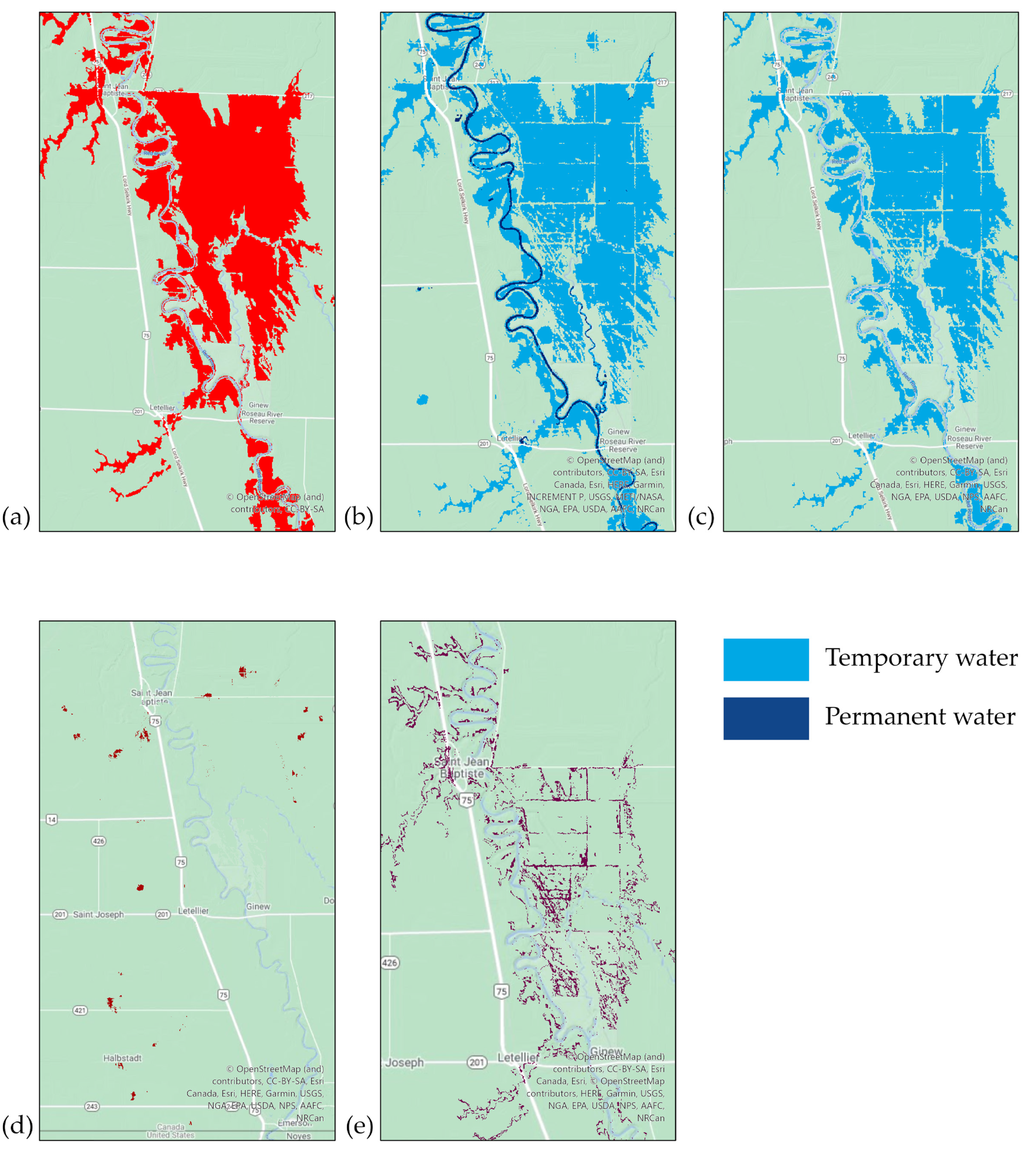
This section uses the 2019 Red River floods for visualization purposes. The reference flood extent is shown in red, permanent water bodies in the dark blue, and flood inundation extent mapped by FMA in light blue.

3.1. Data Cube Density

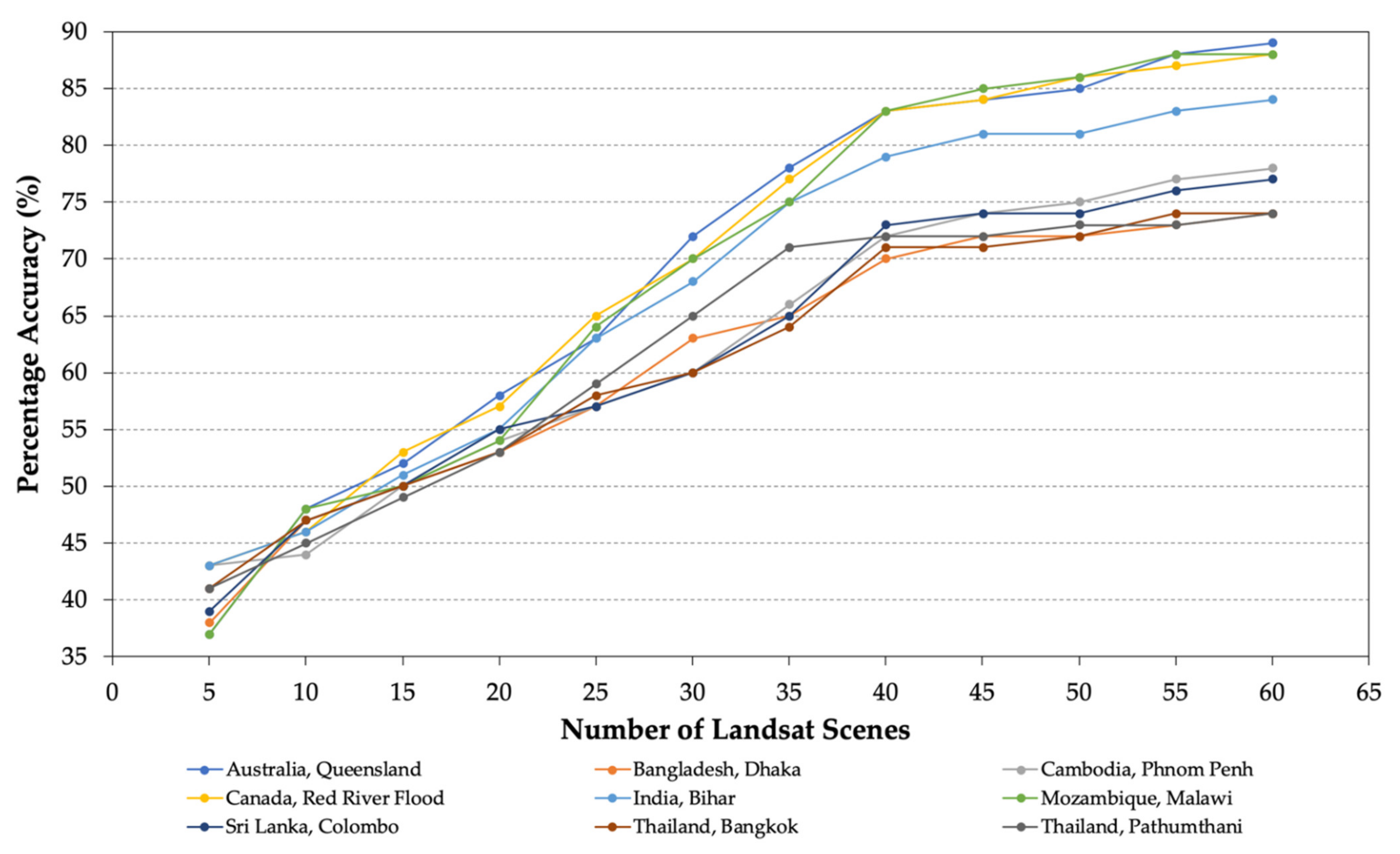
A function is developed in the GEE platform to report on the number of Landsat scenes used to create the data cube for a particular flood event. The FMA requires a minimum of 40–50 Landsat scenes to detect the inundated area with stable accuracy, as shown in Figure 2. During the analysis, the start and end date of the flood event was adjusted to ensure the required number of Landsat scenes are available to construct the data cube.

3.2. MNDWI, NDVI, and HAND

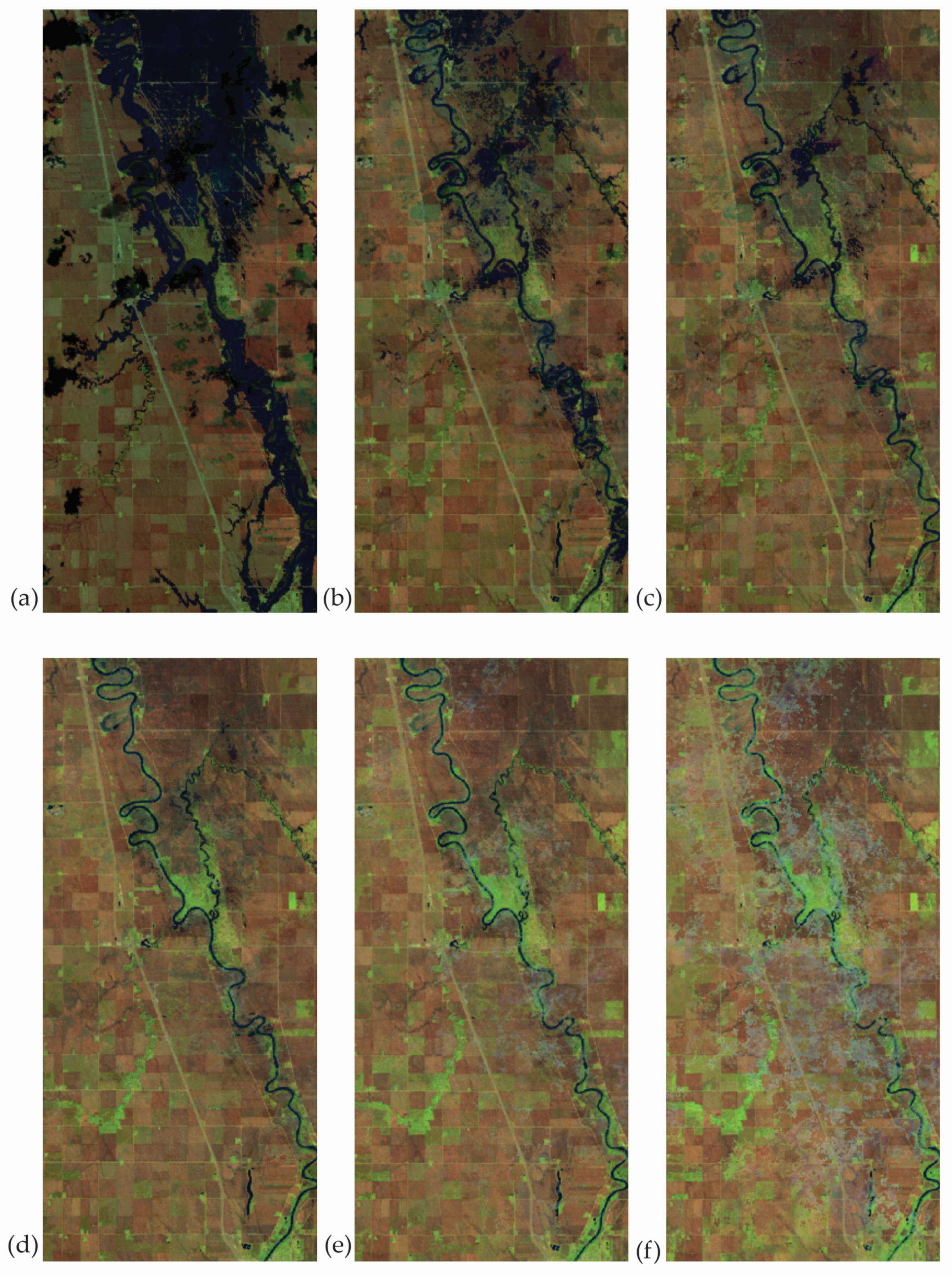
Percentiles are used to identify the temporary water and the permanent water; 10 percentile is used for temporary water and 40 percentile for the permanent water. Figure 3a shows that the lower percentile detects temporary water bodies, and the higher percentile value detects permanent water bodies. However, the percentile above 40 detect features other than water, as shown in Figure 3e,f.
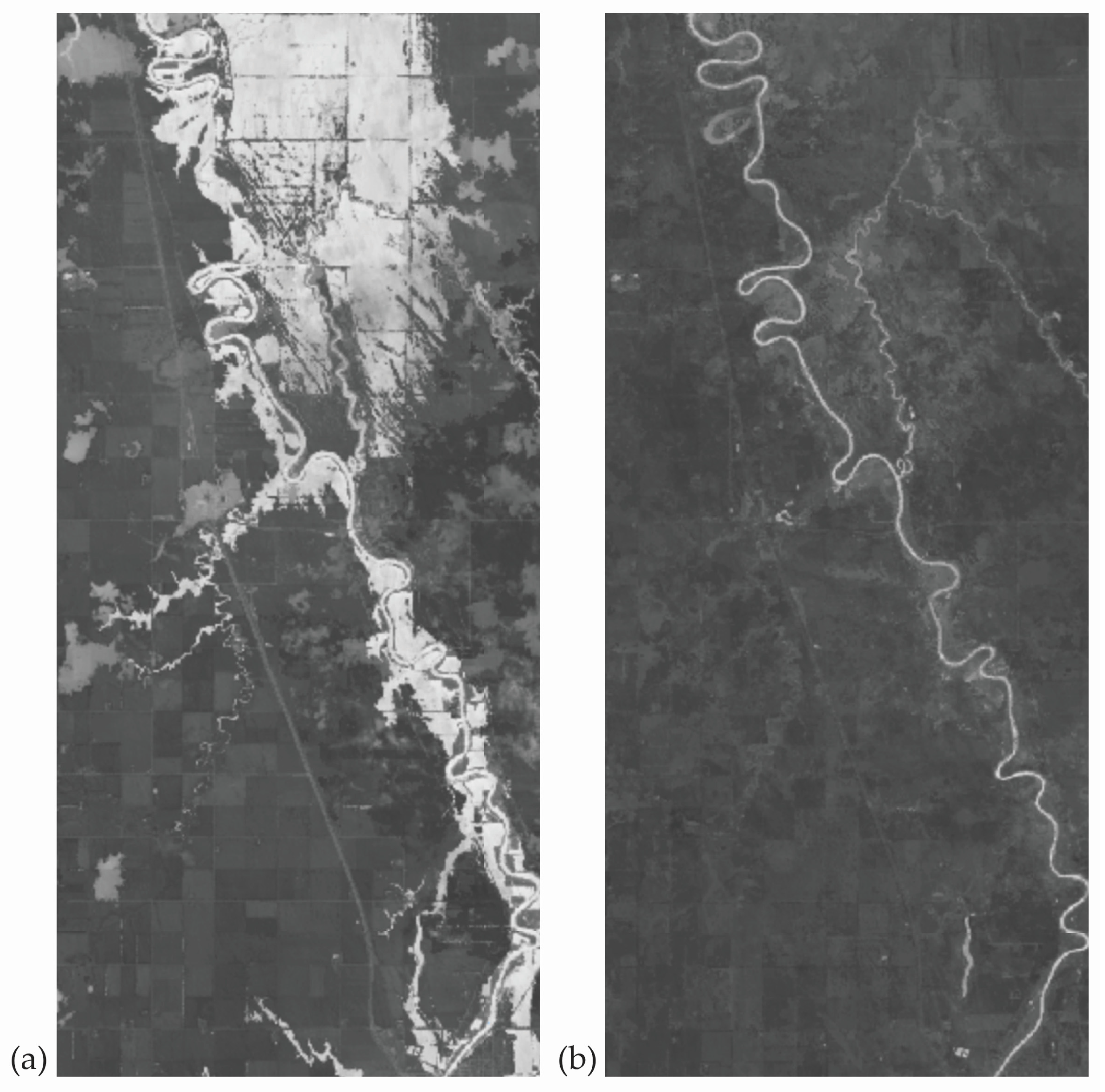
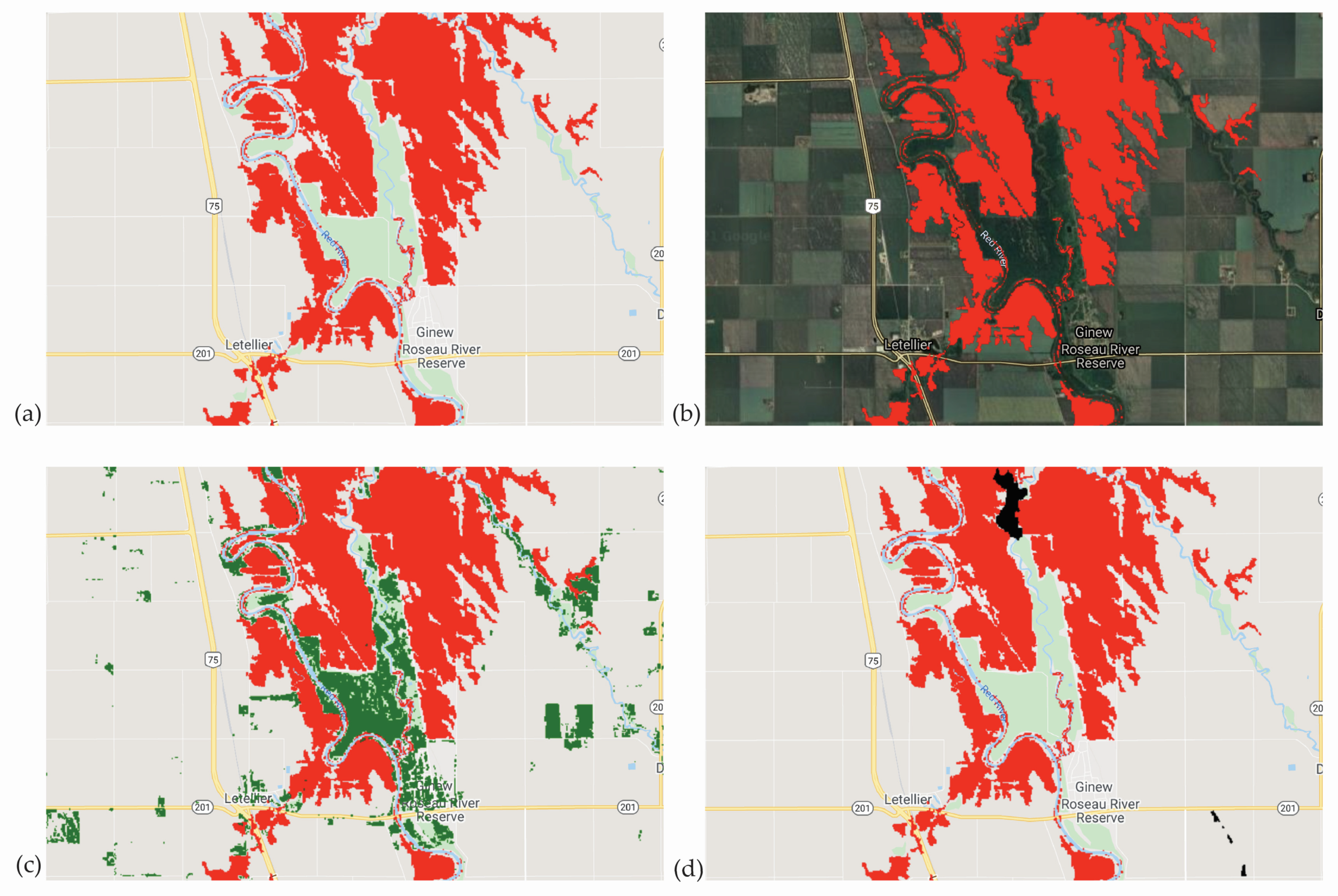
MNDWI is calculated using the percentile images. Figure 4 shows the MNDWI calculated using 10 percentile and 40 percentile images. The temporary and permanent water layers derived from MNDWI are combined in a single ‘water’ layer for a particular flood event. FMA uses a very high threshold (0.4) value of NDVI index to exclude very dark vegetated areas, correction on hill shadows, snow, and ice; this mask is created with an assumption that land with dark vegetation is not flooded. Figure 5 shows the NDVI mask in green and HAND mask in black for the 2019 Red River flood.

3.3. Validation

The results obtained from FMA for the flood events are tabulated in Table 4 and Table 5. The TPR value ranges from 0.71–0.90, indicating that FMA is correctly detecting a high number of flood pixels in the ground truth data as flood. A higher TPR value is observed for flood events in rural areas and having land covers such as rural built-up, rural agriculture, open spaces, and wetland. Queensland flood event has the highest TPR and accuracy as the FMA can detect the flood pixels because of homogenous land cover and absence of tree cover, and large urban structures covering the flood water as observed from space.
The same pattern of higher accuracy (84–89%) and TPR (84–90%) is observed for Red River, Bihar, and Malawi flood events. Figure 6a shows the Red River flood extent used as ground truth data, and Figure 6b shows the flood inundation extent mapped by FMA, a good overlap can be observed between the ground truth data and FMA output with few horizontal and vertical strips not detected as flood by the FMA. These vertical and horizontal stripes are the road network which the ground truth labeled as flooded. The false negative is detected at the flood boundary areas, as shown in Figure 6e; this could be because of the overestimation of the reference data or underestimation by the FMA. In some flood events, the false negative was randomly distributed or was concentrated in urban areas. Soon, a study will be conducted using reference data with higher accuracy supported by ground surveys. As shown in Figure 6d, the false positives are detected outside the boundary of the reference flood map; the behavior is observed for other flood events as well.
As shown in Figure 6c, it is observed that the FMA detects flood with an accuracy that can be used to develop flood monitoring and mapping applications discussed in Section 4.
The accuracy and TPR are lower in areas with a land cover like rural built-up and rural agriculture. Several horizontal and vertical lines can be seen in Figure 6b, which are not detected as flood by FMA. These lines are either road networks, or tree canopy cover. This trend in FMA is also observed for other flood events in the urban environment, including Colombo, Dhaka, Phnom Penh, and Bangkok flood events. However, it is worth noting that despite the underperformance of FMA in the urban environment, the accuracy ranges from 0.74–0.78 for these flood events, which is good enough to develop flood mapping and monitoring applications discussed in Section 4.

4. Discussion

In the last decade, the floods have caused an economic loss of nearly USD 500 B, equal to Singapore’s GDP. Around 1.47 B people are exposed to the risk of intense flooding, which is more than Europe’s total population. The majority of this population segment lives in low and low-middle-income countries, exponentially increasing the disaster-driven socio-economic risk [47].
Developing FEWS and historical flood and risk maps are the two primary approaches to address the food-related challenges. However, developing and deploying such systems in Global South is an expensive and time-consuming exercise. The resource intensiveness of these solutions can be gauged from the fact that if Canada had to update its historical flood maps, it would cost USD 350 M and one decade to complete the exercise [48].
FMA has been designed to address the data and information gaps and challenges in the Global South. This section identifies the possible application areas for FMA; this is not an exhaustive list, and more application areas exist.

4.1. Land Use

Using the FMA in countries with poor or no flood risk maps can help add a new level of robustness to land use planning in such places. Identifying those locations which are at risk of flooding can allow for optimization of resources and investment such as upgrading infrastructure, developing agriculture, etc., in the short term. In the medium to longer-term, land-use planning can benefit from knowledge on where detailed flood studies are required if growth is to be sustained in a given location.

4.2. Emergency Services

Metrics such as investment in public infrastructure, natural disaster-related insurance rates, flood-related human and economic losses, etc., can be estimated using FMA. The flood inundation extents are also available as an interoperable service that can be merged with other open datasets for decision making.
In developing countries and emerging economies, data collection of hydrological and other environmental variables is rarely a priority. This activity is often compounded by difficult terrain or cost barriers to technology and tools [49,50]. EO data is a simple solution to this problem in the short term, allowing those most vulnerable but poorly gauged locations to be observed. From these observations, low-resolution flood risk models can be generated. This will enable governments, funding agencies, and disaster management authorities to hone-in on the highest potential risk locations and generate higher resolution models. In addition, this methodology allows users to justify investment in higher resolution models around high-risk settlements and assets. In time this strengthens the ability of these countries to better plan for and respond to disasters.

4.3. Insurance

The use and value of remotely sensed risk information in the insurance industry is not new [51,52]. There were significant losses/damage to property and agricultural concerns in several of the flood events above. In the case of Queensland, Australia, huge insurance payouts had to be made. In poorer nations such as Cambodia and Bangladesh, this safety blanket did not exist, and many livelihoods and homes were permanently lost due to flood events. FMA could be part of the conversation between governments/international donor organizations and the insurance industry generating agriculture insurance support for persons living and farming at the subsistence level. Creating this safety net and closing this gap in financial security has far-reaching implications for global development goals and promoting more secure economies and nations.

5. Conclusions

An algorithm for flood inundation extent mapping using GEE is proposed, utilizing EO data to map any flood event from 1985-present. FMA can be an effective supplement to current inundation and flood risk maps, especially in the Global South, where data and technological gaps are common. FMA can also be used in an exploratory capacity prior to flood mapping, as it is significantly lower in cost, only requiring access to the internet and using open-source EO data. There are some limitations where the terrain influences the accuracy of the outputs, but these are easily characterized and can be further calibrated and accounted for with more event inputs. The FMA can be used to create historical flood inundation maps and potential flood risk maps. Room exists to improve this product with the addition of other remotely sensed datasets.
Additional aspects we hope to study include integrating Sentinel-2 data into the FMA workflow to increase the model performance and combining the FMA output with the demographic and utility data available under open access to create a comprehensive tool to convey the impacts of flooding in an area.

Author Contributions

Conceptualization, H.M. and D.P.; methodology, H.M.; formal analysis H.M. and C.C.; writing—original draft preparation, H.M. and C.C.; writing—review and editing, H.M., C.C. and D.P. All authors have read and agreed to the published version of the manuscript.

Funding

This research is supported by the funds received by UNU-INWEH through the long-term agreement with Global Affairs Canada. The year 2021 marks the 25-th anniversary of UNU-INWEH.

Institutional Review Board Statement

Not applicable.

Informed Consent Statement

Not applicable.

Data Availability Statement

The Google Earth engine script, ground truth data, and FMA outputs may be made available on request from the authors.

Acknowledgments

UNU INWEH would like to acknowledge the funding and support of Global Affairs Canada to its research, policy, and development mandate, programs, and projects.

Conflicts of Interest

The authors declare no conflict of interest.

References

  1. Perera, D.; Seidou, O.; Agnihotri, J.; Rasmy, M.; Smakhtin, V.; Coulibaly, P.; Mehmood, H. Flood Early Warning Systems: A Review of Benefits, Challenges and Prospects; United Nations University, Institute for Water, Environment and Health: Hamilton, ON, Canada, 2019. [Google Scholar]
  2. Podlaha, A.; Lörinc, M.; Bhattacharya, A.; Bowen, S. Weather, climate & catastrophe insight. Annu. Rep. 2018, 1, 4–10. [Google Scholar]
  3. IFRC. 17.5 Million Affected by Floods and Threatened by Disease in South Asia. Available online: https://media.ifrc.org/ifrc/press-release/17-5-million-affected-floods-threatened-disease-south-asia/ (accessed on 20 January 2021).
  4. Coumou, D.; Rahmstorf, S. A decade of weather extremes. Nat. Clim. Chang. 2012, 2, 491–496. [Google Scholar] [CrossRef]
  5. Werner, M.G.F. A comparison of flood extent modelling approaches through constraining uncertainties on gauge data. Hydrol. Earth Syst. Sci. 2004, 8, 1141–1152. [Google Scholar] [CrossRef] [Green Version]
  6. Di Baldassarre, G.; Schumann, G.; Bates, P.D. A technique for the calibration of hydraulic models using uncertain satellite observations of flood extent. J. Hydrol. 2009, 367, 276–282. [Google Scholar] [CrossRef]
  7. Priestnall, G.; Jaafar, J.; Duncan, A. Extracting urban features from LiDAR digital surface models. Comput. Environ. Urban Syst. 2000, 24, 65–78. [Google Scholar] [CrossRef]
  8. Galland, J.-C.; Goutal, N.; Hervouet, J.-M. TELEMAC: A new numerical model for solving shallow water equations. Adv. Water Resour. 1991, 14, 138–148. [Google Scholar] [CrossRef]
  9. Sinha, S.K.; Sotiropoulos, F.; Odgaard, A.J. Three-dimensional numerical model for flow through natural rivers. J. Hydraul. Eng. 1998, 124, 13–24. [Google Scholar] [CrossRef]
  10. Wing, O.E.J.; Bates, P.D.; Smith, A.M.; Sampson, C.C.; Johnson, K.A.; Fargione, J.; Morefield, P. Estimates of present and future flood risk in the conterminous United States. Environ. Res. Lett. 2018, 13, 034023. [Google Scholar] [CrossRef]
  11. The Globe and Mail Poor Flood Risk Maps or None at All Keeping are Keeping Communities in Flood Prone Areas. Available online: https://www.theglobeandmail.com/canada/article-poor-flood-risk-maps-or-none-at-all-are-keeping-canadian-communities/ (accessed on 20 January 2021).
  12. Institute of Catastrophic Loss Reduction. Focus on Flood Mapping in Canada; Institute of Catastrophic Loss Reduction: Toronto, ON, Canada, 2019. [Google Scholar]
  13. Perera, D.; Seidou, O.; Agnihotri, J.; Mehmood, H.; Rasmy, M. Challenges and technical advances in flood early warning systems (FEWSs). In Flood Impact Mitigation and Resilience Enhancement; InTech: London, UK, 2020. [Google Scholar]
  14. Wulder, M.A.; Masek, J.G.; Cohen, W.B.; Loveland, T.R.; Woodcock, C.E. Opening the archive: How free data has enabled the science and monitoring promise of Landsat. Remote Sens. Environ. 2012, 122, 2–10. [Google Scholar] [CrossRef]
  15. Lewis, A.; Lymburner, L.; Purss, M.B.J.; Brooke, B.; Evans, B.; Ip, A.; Dekker, A.; Irons, J.R.; Minchin, S.; Mueller, N.; et al. Rapid, high-resolution detection of environmental change over continental scales from satellite datathe Earth Observation Data Cube. Int. J. Digit. Earth 2016, 9, 106–111. [Google Scholar] [CrossRef]
  16. Gorelick, N.; Hancher, M.; Dixon, M.; Ilyushchenko, S.; Thau, D.; Moore, R. Google Earth engine: Planetary-scale geospatial analysis for everyone. Remote Sens. Environ. 2017, 202, 18–27. [Google Scholar] [CrossRef]
  17. Saah, D.; Tenneson, K.; Matin, M.; Uddin, K.; Cutter, P.; Poortinga, A.; Nguyen, Q.H.; Patterson, M.; Johnson, G.; Markert, K.; et al. Land cover mapping in data scarce environments: Challenges and opportunities. Front. Environ. Sci. 2019, 7. [Google Scholar] [CrossRef] [Green Version]
  18. Phongsapan, K.; Chishtie, F.; Poortinga, A.; Bhandari, B.; Meechaiya, C.; Kunlamai, T.; Aung, K.S.; Saah, D.; Anderson, E.; Markert, K.; et al. Operational flood risk index mapping for disaster risk reduction using earth observations and cloud computing technologies: A case study on Myanmar. Front. Environ. Sci. 2019, 7. [Google Scholar] [CrossRef] [Green Version]
  19. Poortinga, A.; Nguyen, Q.; Tenneson, K.; Troy, A.; Saah, D.; Bhandari, B.; Ellenburg, W.L.; Aekakkararungroj, A.; Ha, L.; Pham, H.; et al. Linking earth observations for assessing the food security situation in Vietnam: A landscape approach. Front. Environ. Sci. 2019, 7. [Google Scholar] [CrossRef] [Green Version]
  20. Patel, N.N.; Angiuli, E.; Gamba, P.; Gaughan, A.; Lisini, G.; Stevens, F.R.; Tatem, A.J.; Trianni, G. Multitemporal settlement and population mapping from Landsat using Google Earth engine. Int. J. Appl. Earth Obs. Geoinf. 2015, 35, 199–208. [Google Scholar] [CrossRef] [Green Version]
  21. Mutanga, O.; Kumar, L. Google Earth engine applications. Remote Sens. 2019, 11, 591. [Google Scholar] [CrossRef] [Green Version]
  22. IWM. Flood Risk Mapping: South Asia. Available online: http://waterdata.iwmi.org/Applications/Catastrophic_Flood_Risk_Mapping/ (accessed on 20 January 2021).
  23. Pekel, J.-F.; Cottam, A.; Gorelick, N.; Belward, A.S. High-resolution mapping of global surface water and its long-term changes. Nature 2016, 540, 418–422. [Google Scholar] [CrossRef] [PubMed]
  24. Vanama, V.S.K.; Mandal, D.; Rao, Y.S. GEE4FLOOD: Rapid mapping of flood areas using temporal Sentinel-1 SAR images with Google Earth engine cloud platform. J. Appl. Remote Sens. 2020, 14, 1. [Google Scholar] [CrossRef]
  25. DeVries, B.; Huang, C.; Armston, J.; Huang, W.; Jones, J.W.; Lang, M.W. Rapid and robust monitoring of flood events using Sentinel-1 and Landsat data on the Google Earth engine. Remote Sens. Environ. 2020, 240, 111664. [Google Scholar] [CrossRef]
  26. Manfreda, S.; Samela, C. A digital elevation model based method for a rapid estimation of flood inundation depth. J. Flood Risk Manag. 2019, 12. [Google Scholar] [CrossRef] [Green Version]
  27. Mosavi, A.; Ozturk, P.; Chau, K.-W. Flood prediction using machine learning models: Literature review. Water 2018, 10, 1536. [Google Scholar] [CrossRef] [Green Version]
  28. Housman, I.A.; Stam, C. Mask Clouds and Cloud Shadows in Landsat Data and Export Composite. 2020. Available online: https://ee-api.appspot.com/a432bf20510f37ce13e847e4394aee77 (accessed on 10 May 2021).
  29. Housman, I.W.; Chastain, R.A.; Finco, M.V. An evaluation of forest health insect and disease survey data and satellite-based remote sensing forest change detection methods: Case studies in the United States. Remote Sens. 2018, 10, 1184. [Google Scholar] [CrossRef] [Green Version]
  30. Ustin, S.L.; Roberts, D.A.; Pinzon, J.; Jacquemoud, S.; Gardner, M.; Scheer, G.; Castañeda, C.M.; Orueta, A.P. Estimating canopy water content of chaparral shrubs using optical methods. Remote Sens. Environ. 1998, 65, 280–291. [Google Scholar] [CrossRef]
  31. Xu, H. Modification of normalised difference water index (NDWI) to enhance open water features in remotely sensed imagery. Int. J. Remote Sens. 2006, 27, 3025–3033. [Google Scholar] [CrossRef]
  32. Acharya, T.D.; Subedi, A.; Lee, D.H. Evaluation of water indices for surface water extraction in a Landsat 8 scene of Nepal. Sensors 2018, 18, 2580. [Google Scholar] [CrossRef] [PubMed] [Green Version]
  33. Donchyts, G.; Winsemius, H.; Schellekens, J.; Erickson, T.; Gao, H.; Savenije, H.; van de Giesen, N. Global 30 m height above the nearest drainage. In Proceedings of the EGU General Assembly Conference, Vienna, Austria, 17–22 April 2016. [Google Scholar]
  34. Deng, Y.; Jiang, W.; Tang, Z.; Ling, Z.; Wu, Z. Long-term changes of open-surface water bodies in the Yangtze River basin based on the Google Earth engine cloud platform. Remote Sens. 2019, 11, 2213. [Google Scholar] [CrossRef] [Green Version]
  35. Hansen, M.C.; Potapov, P.V.; Moore, R.; Hancher, M.; Turubanova, S.A.; Tyukavina, A.; Thau, D.; Stehman, S.V.; Goetz, S.J.; Loveland, T.R.; et al. High-resolution global maps of 21st-century forest cover change. Science 2013, 342, 850–853. [Google Scholar] [CrossRef] [Green Version]
  36. Martz, L.; Garbrecht, J. Numerical definition of drainage network and subcatchment areas from Digital Elevation Models. Comput. Geosci. 1992, 18, 747–761. [Google Scholar] [CrossRef]
  37. Nobre, A.D.; Cuartas, L.A.; Momo, M.R.; Severo, D.L.; Pinheiro, A.; Nobre, C.A. HAND contour: A new proxy predictor of inundation extent. Hydrol. Process. 2016, 30, 320–333. [Google Scholar] [CrossRef]
  38. Donchyts, G.; Winsemius, H.; Schellekens, J.; Erickson, T.; Gao, H.; Savenije, H.; van de Giesen, N. Global 30 m Height above the Nearest Drainage. 2016. Available online: https://samapriya.github.io/awesome-gee-community-datasets/projects/hand/ (accessed on 10 May 2021).
  39. Bureau of Meteorology, Australian Government. Report on Queensland Floods; Bureau of Meteorology: Longreach, QLD, Australia, 2008.
  40. National Climate Change Adaptation Research Facility. Extreme Rainfall and Flood Event in Mackay on 1 February 2008. Snapshot for CoastAdapt; National Climate Change Adaptation Research Facility: Southport, QLD, Australia, 2016. [Google Scholar]
  41. Trade and Markets Division Food and Agriculture Organisation (FAO). Global Information and Early Warning on Food and Agri-Culture (GIEWS) Update Bangladesh Floods; FAO: Rome, Italy, 2017. [Google Scholar]
  42. International Federation of Red Cross and Red Crescent (IFRC). DREF Operation Final Report: Cambodia Floods; International Federation of Red Cross and Red Crescent: Geneva, Switzerland, 2012. [Google Scholar]
  43. The Wire India Floods in Bihar Destroyed 7.54 Lakh Hectares of Agricultural Land This Year. Available online: https://thewire.in/environment/floods-bihar-agricultural-land (accessed on 25 April 2021).
  44. Floodlist Malawi and Mozambique—Death Toll Rises after Widespread Flooding. Available online: http://floodlist.com/africa/malawi-mozambique-floods-march-2019 (accessed on 25 April 2021).
  45. ReliefWeb. Sri Lanka: Floods and Landslides Situation Report No. 2; United Nations Office for the Coordination of Humanitarian Affairs: New York, NY, USA, 2016. [Google Scholar]
  46. Gale, E.L.; Saunders, M.A. The 2011 Thailand flood: Climate causes and return periods. Weather 2013, 68, 233–237. [Google Scholar] [CrossRef] [Green Version]
  47. Rentschler, J.; Salhab, M. People in Harm’s Way: Flood Exposure and Poverty in 189 Countries; World Bank Group: Washington, DC, USA, 2020; pp. 1–28. [Google Scholar]
  48. Braden, J.; Simonovic, S.P. A Review of Flood Hazard Mapping Practices across Canada; University of West Ontario, Department of Civil and Environmental Engineering: London, ON, Canada, 2020; ISBN 978-0-7714-3143-2. [Google Scholar]
  49. Sivapalan, M.; Takeuchi, K.; Franks, S.; Gupta, V.K.; Karambiri, H.; Lakshmi, V.; Liang, X.; Mcdonnell, J.; Mendiondo, E.M.; O’Connell, P.E.; et al. IAHS decade on predictions in ungauged basins (PUB), 2003–2012: Shaping an exciting future for the hydrological sciences. Hydrol. Sci. J. 2003, 48, 857–880. [Google Scholar] [CrossRef] [Green Version]
  50. Grimes, D.; Pardo-Iguzquiza, E.; Bonifacio, R. Optimal areal rainfall estimation using raingauges and satellite data. J. Hydrol. 1999, 222, 93–108. [Google Scholar] [CrossRef]
  51. Rumson, A.G.; Hallett, S. Innovations in the use of data facilitating insurance as a resilience mechanism for coastal flood risk. Sci. Total. Environ. 2019, 661, 598–612. [Google Scholar] [CrossRef]
  52. De Leeuw, J.; Vrieling, A.; Shee, A.; Atzberger, C.; Hadgu, K.M.; Biradar, C.M.; Keah, H.; Turvey, C. The potential and uptake of remote sensing in insurance: A review. Remote Sens. 2014, 6, 10888–10912. [Google Scholar] [CrossRef] [Green Version]
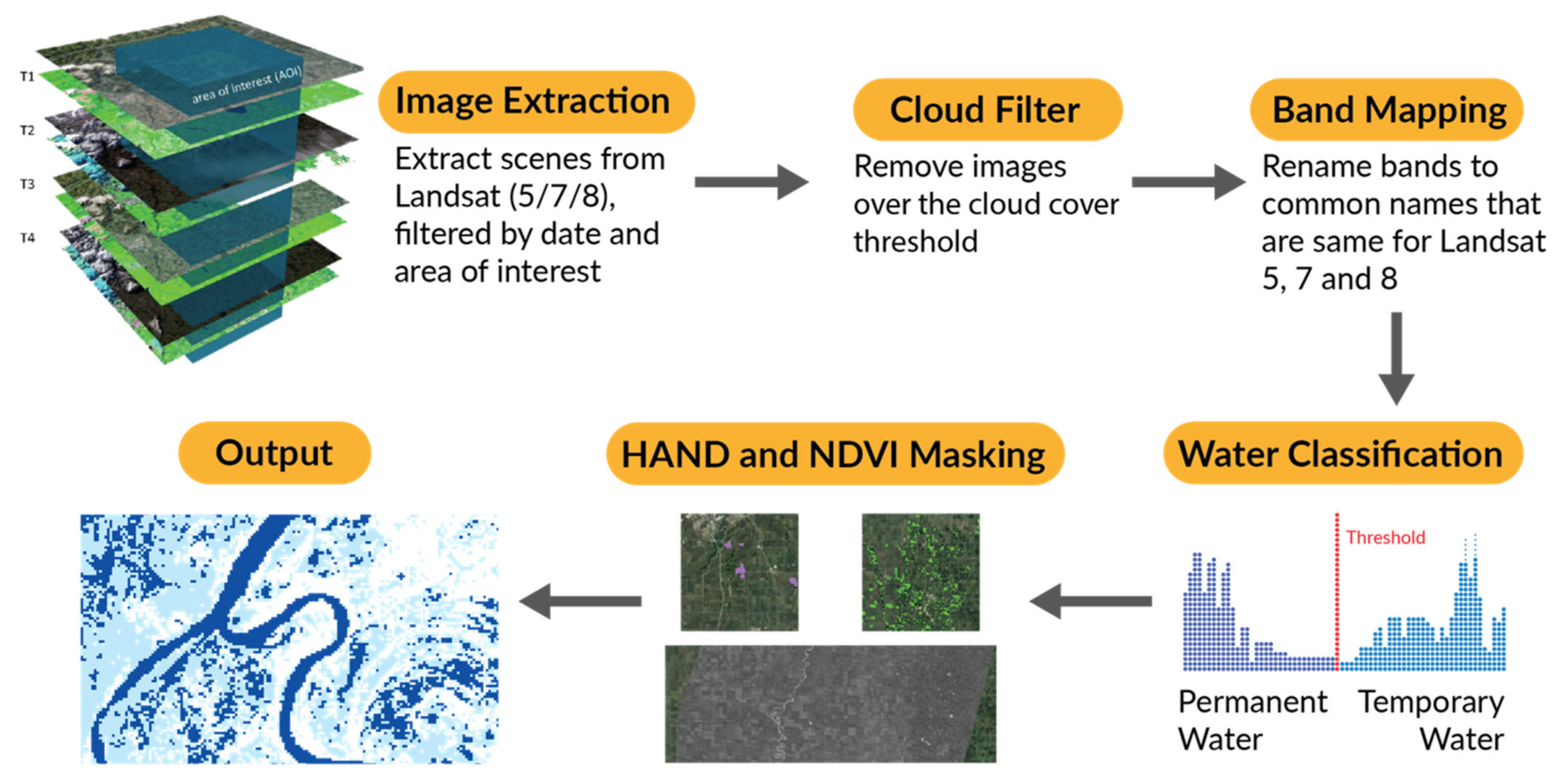
Figure 1. Schematic workflow for flood mapping in GEE using Landsat 5, 7, and 8.
Atmosphere 12 00866 g001
Figure 2. Relationship between the FMA accuracy and number of Landsat scenes used to construct the data cube.
Atmosphere 12 00866 g002
Figure 3. Intensity percentile false-color images for 2019 Red River flood (a) 10 percentile; (b) 20 percentile; (c) 30 percentile; (d) 40 percentile; (e) 50 percentile; (f) 60 percentile.
Atmosphere 12 00866 g003
Figure 4. MNDWI for (a) 10 percentile (temporary water); (b) 40 percentile images (permanent water).
Atmosphere 12 00866 g004
Figure 5. NDVI and HAND mask for 2019 Red River flood. (a) reference flood extent with vegetation marked on Google Maps; (b) reference flood extent with vegetation visible of satellite imagery; (c) reference flood extent with NDVI mask (threshold set at 0.4); (d) reference flood extent with HAND mask (threshold set at 0.4).
Atmosphere 12 00866 g005
Figure 6. FMA inputs and outputs for 2019 Red River Flood (a) reference flood extent; (b) flood inundation extent mapped by FMA; (c) true positive; (d) false positive; (e) false negative.
Atmosphere 12 00866 g006
Table 1. Characteristics of the Landsat sensors used in the study.
SatelliteSensorLaunch YearResolution
Landsat 5MSS/TM198430 m
Landsat 7ETM+199930 m
Landsat 8OLI/TIRS201330 m
Table 2. Location, event, and data source for each flood event used for validation.
Country, CityYearData Source
Australia, Queensland2008Dartmouth Flood Observatory, University of Colorado
Bangladesh, Dhaka2014Copernicus, Emergency Management Service
Canada, Red River2019Natural Resources Canada
Cambodia, Phnom Penh2011Governmental Information Technology Development Agency, Thailand
India, Bihar2017Dartmouth Flood Observatory, University of Colorado
Mozambique, Malawi2015The Humanitarian Data Exchange
Sri Lanka, Colombo2016Irrigation Department, Sri Lanka
Thailand, Pathumthani2011Governmental Information Technology Development Agency, Thailand
Thailand, Bangkok2011Governmental Information Technology Development Agency, Thailand
Table 3. Performance indices for FMA.
IndexDescription
True positive ( T p )Number of flood pixels in the ground truth data detected as flood by FMA
True negative ( T n )Number of non-flood pixels in the ground truth data detected as non-flood by FMA
False positive ( F p )Number of non-flood pixels in the ground truth data detected as flood by FMA
False negative ( F n )Number of flood pixels in the ground truth data detected as non-flood by FMA
Table 4. FMA performance metrics for the flood events (number of pixels, 30 m resolution).
Country, CityTpTnFpFn
Australia, Queensland8,703,4251,921,535339,0941,017,283
Bangladesh, Dhaka3,480,371902,318171,8701,331,994
Canada, Red River137,64522,941183520,647
Cambodia, Phnom Penh31,846,9608,685,534804,21610,615,653
India, Bihar1,904,012469,82186,546370,911
Mozambique, Malawi983,934226,03926,593146,261
Sri Lanka, Colombo767,032108,17119,667245,844
Thailand, Pathumthani640,674186,86326,695266,948
Thailand, Bangkok1,125,724354,68061,683447,205
Table 5. FMA performance metrics for flood events.
Country, CityTPRFPRAccuracyError Rate
Australia, Queensland0.900.150.890.11
Bangladesh, Dhaka0.720.160.740.26
Canada, Red River0.870.070.880.12
Cambodia, Phnom Penh0.750.080.780.22
India, Bihar0.840.160.840.16
Mozambique, Malawi0.870.110.880.14
Sri Lanka, Colombo0.760.150.770.23
Thailand, Pathumthani0.710.130.740.26
Thailand, Bangkok0.720.150.740.26
Publisher’s Note: MDPI stays neutral with regard to jurisdictional claims in published maps and institutional affiliations.