
Experimental Evaluation of PSO Based Transfer Learning Method for Meteorological Visibility Estimation


Abstract
:1. Introduction
2. Methodology
2.1. Related Work
2.2. Particle Swarm Optimization (PSO) Approach
- Pi and Φibest are its own best experience, position and objective value.
- Pg and Φgbest are best experience of the whole swarm, position and objective value.
- ω is the inertia weight, C1 and C2 are cognitive and social acceleration coefficients.
- r1d and r2d are random numbers in [0,1]. Np is the population size.
- Xik ∈ {0,1}, Xik = 1 ⇒ the kth feature value is selected in the ith particle, the total number of “1” in Xi vector is kept constant at 80% of maximum feature dimension (n).
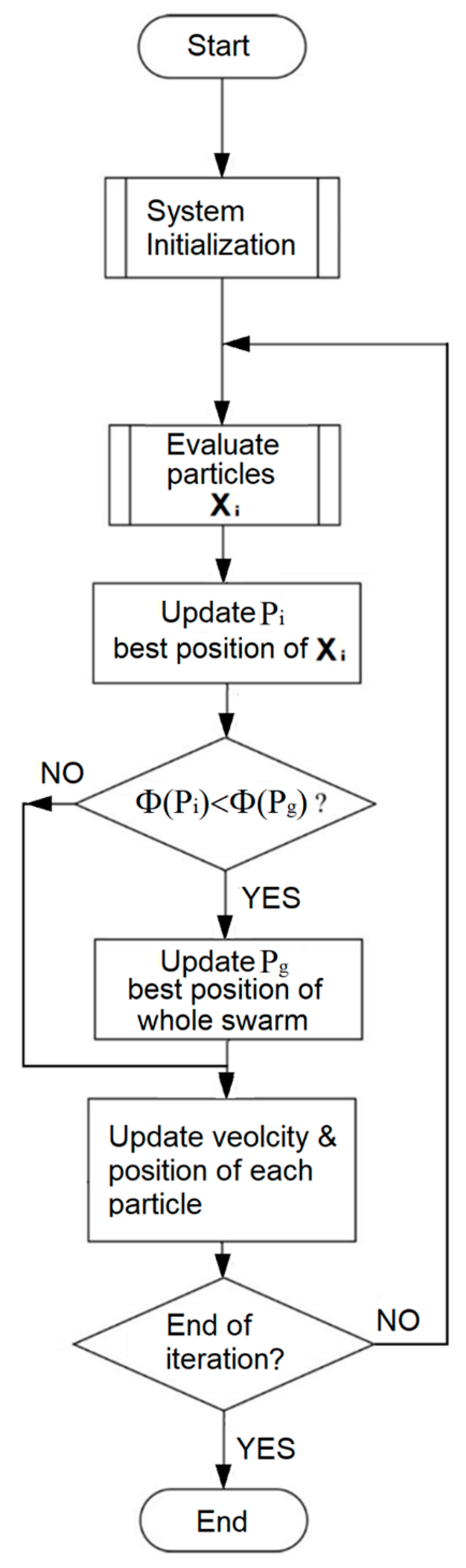
- Initialize the particles’ velocities Vi and positions Xi.
- Updated particles’ Vi velocities and positions Xi by Equations (4) and (5).
- Compare the estimated visibility () with the actual visibility (vj) for all the database images (j = 1…N). Compute the objective values ΦXi for each particle Xi by Equation (1).
- Update the best position Pi and the best objective value Φibest for each particle Xi.
- Update the global best position Pg and the global best objective value Φgbest.
- Go back to step 2 to 5 for updating cycle until maximum generation is reached.
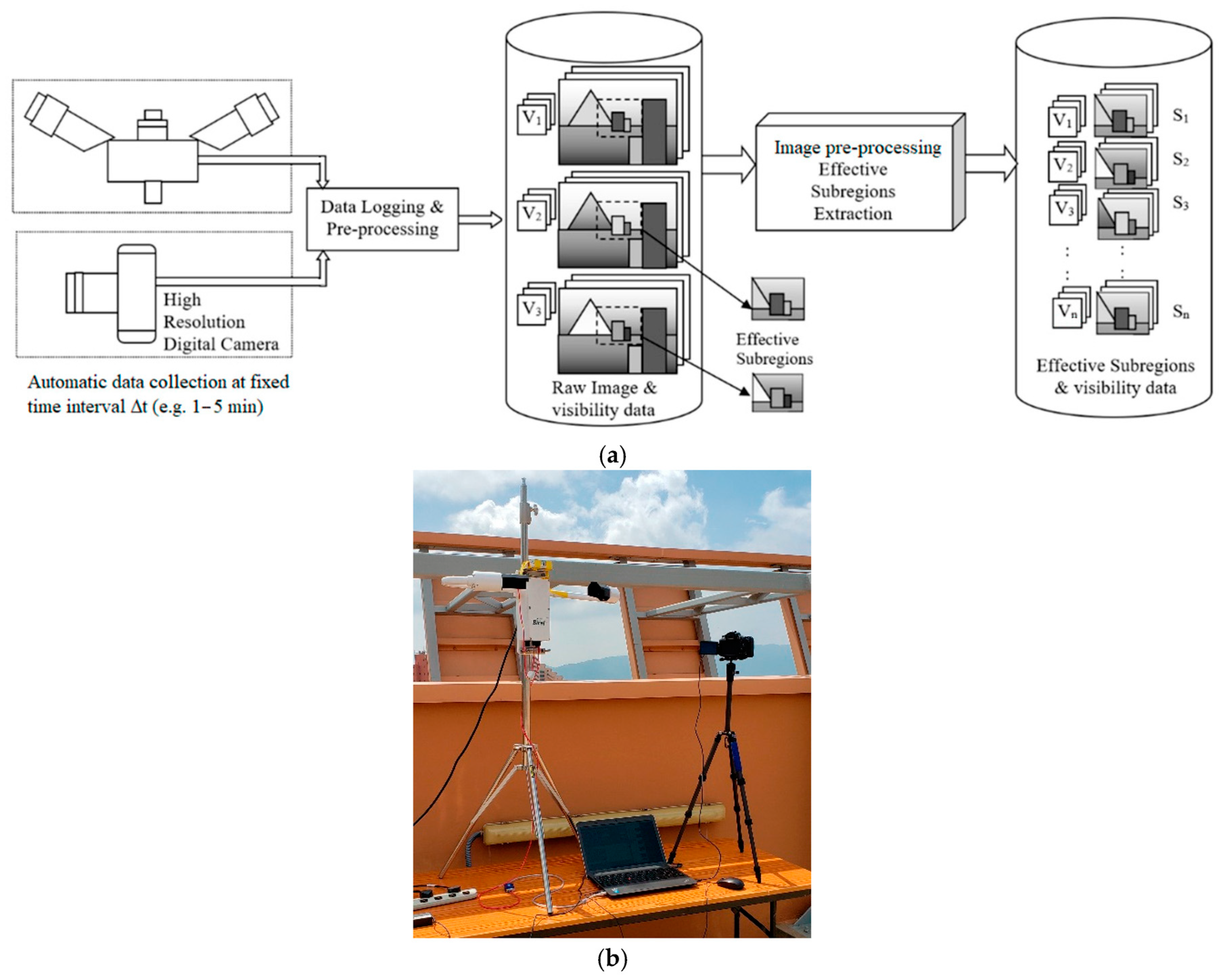
2.3. Database Construction
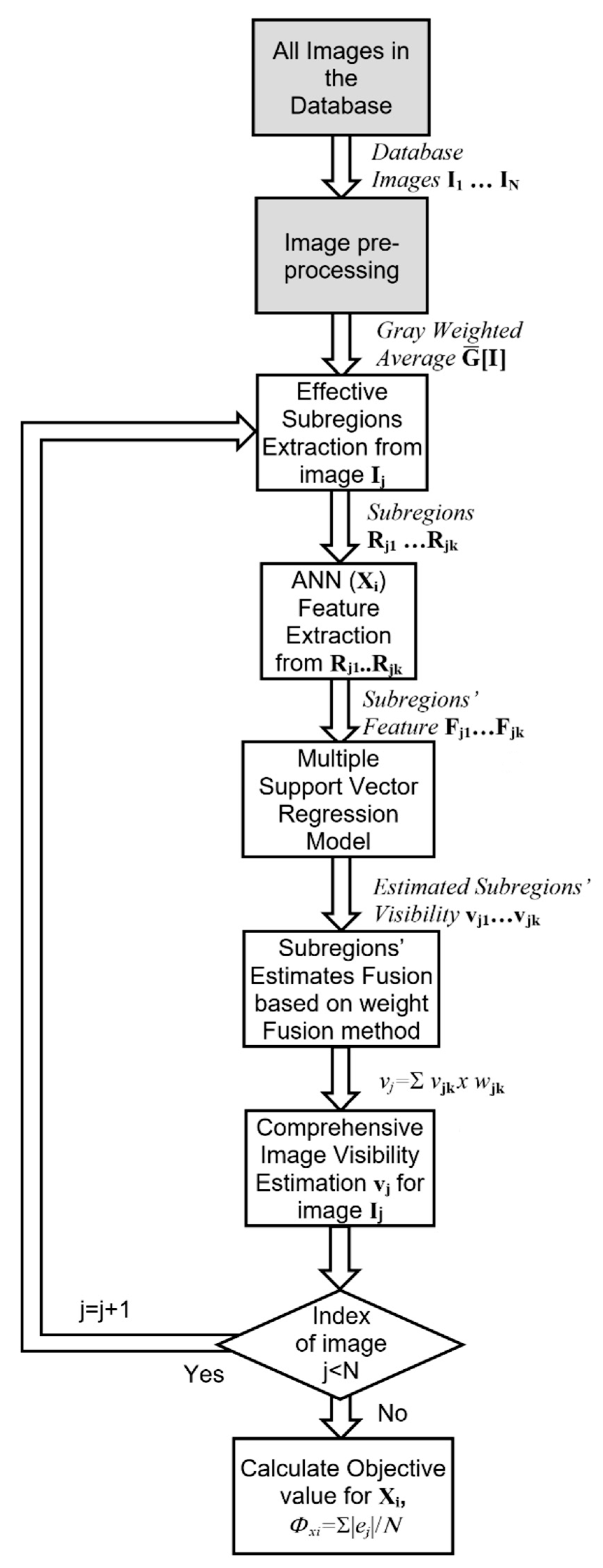
2.4. Method Overview
2.4.1. Image Preprocessing
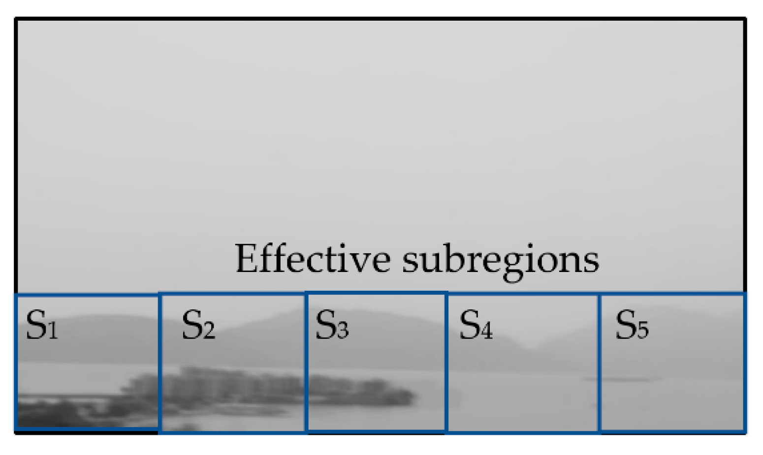
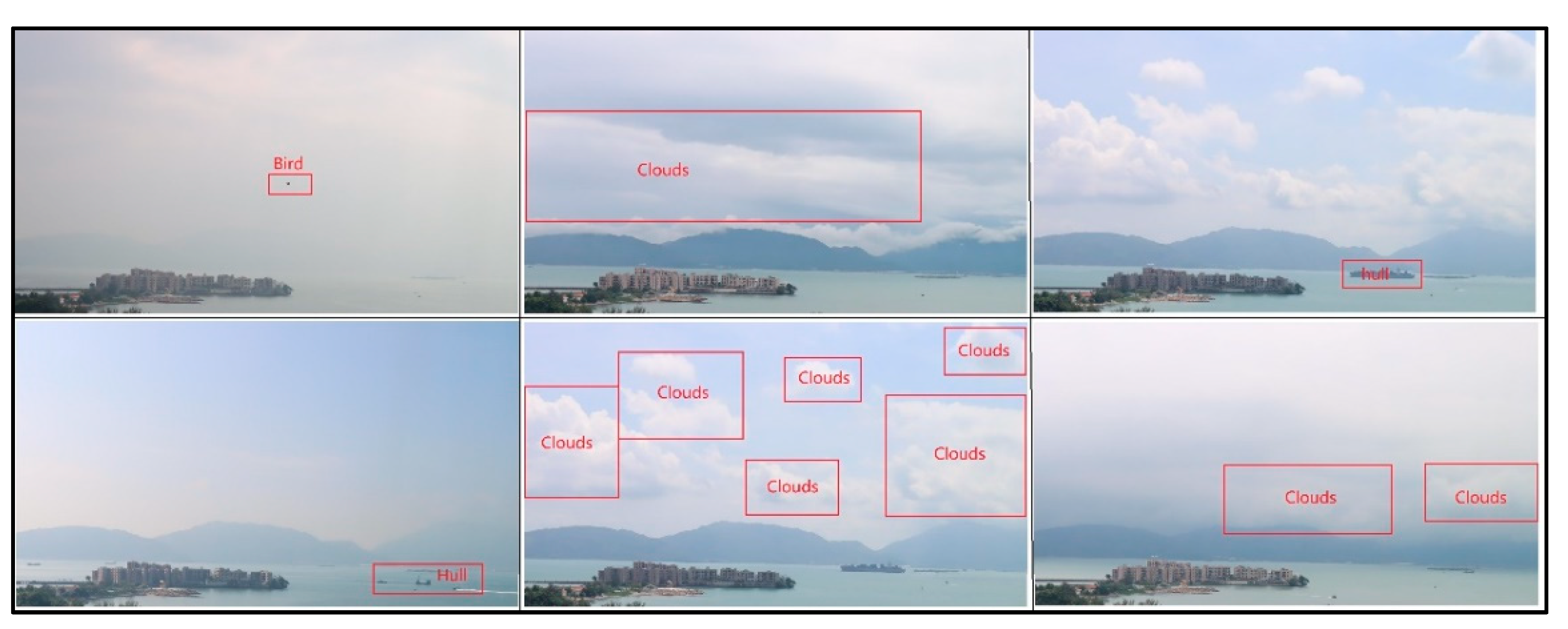
2.4.2. Effective Subregions’ Extraction
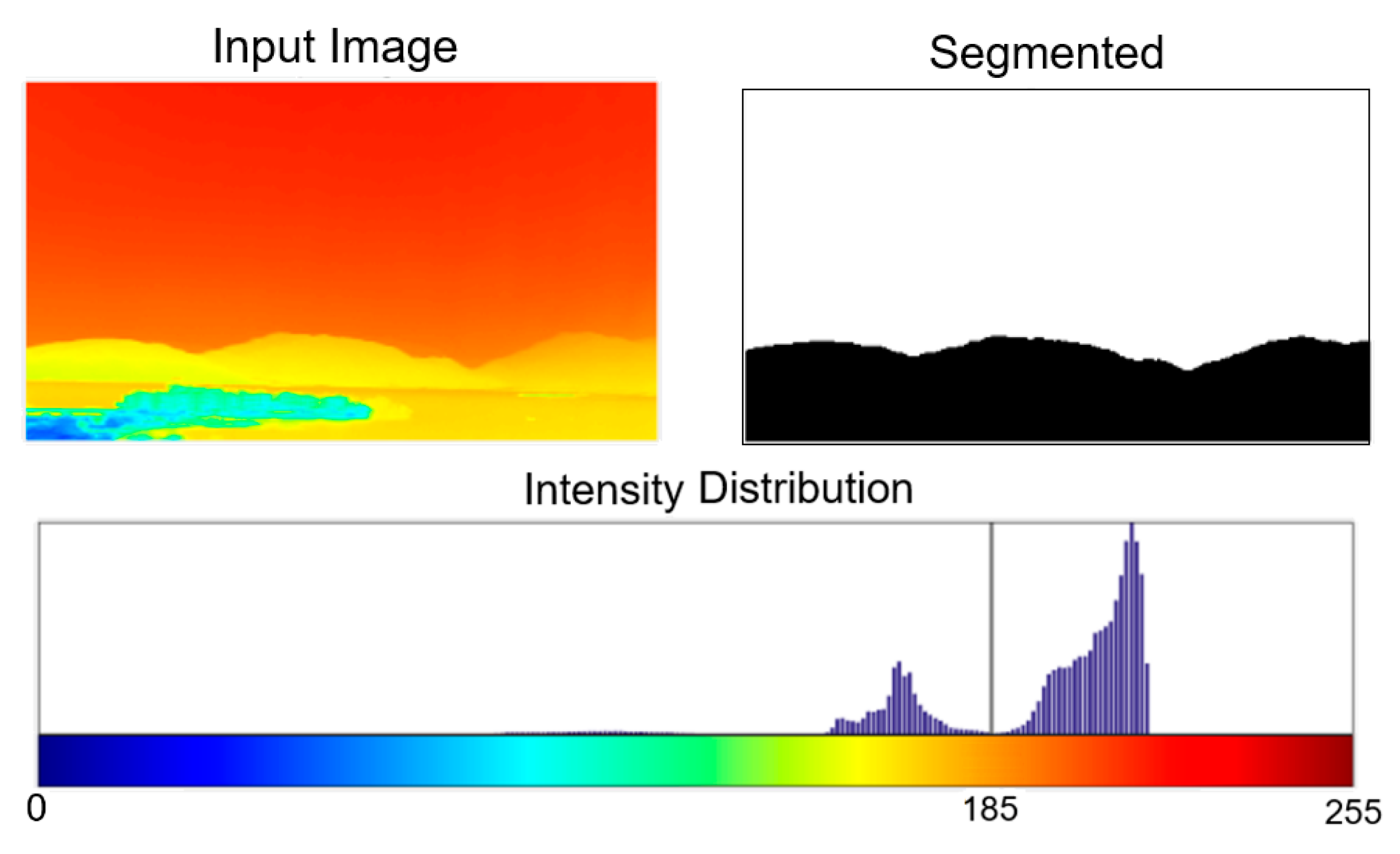
- Apply gray-level averaging to all the images in the database, derive the comprehensive image [I].
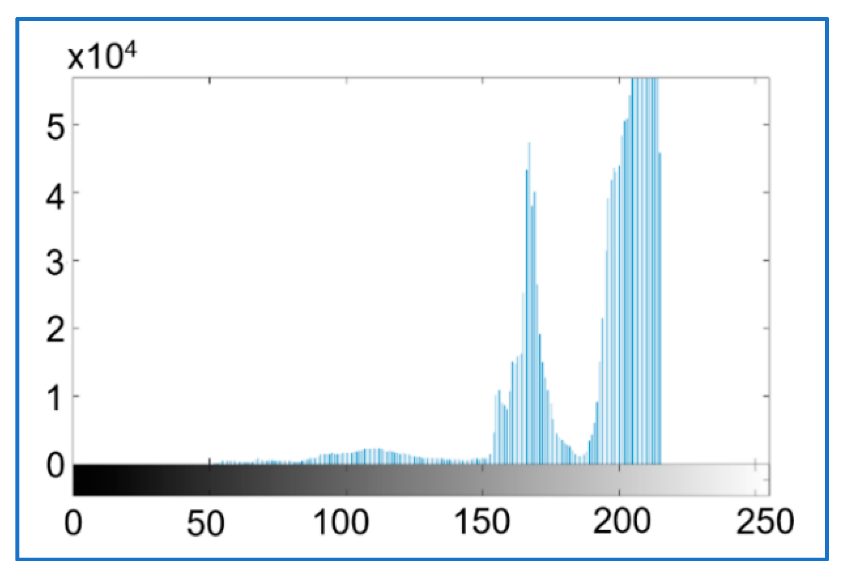
- Generate the grayscale distribution of [I], search the gray level distribution curve from 0 to find the local maximum pk (or peak) of the distribution curve. The local minimum between the first highest maximum p1 and the second highest maximum p2 (or peak) is selected as the threshold gray level (δ).
- Apply the adaptive threshold segmentation algorithm to [I] to obtain an output image. Scan the output image from the top to bottom to search the y level (ymin) for which the pixel’s gray level start to exceed the threshold. Scan the output image from bottom to top to search the y level (ymax) for which the gray level exceeds the threshold.
- The image area S of gray level higher δ is then equally subdivided into subregions Si (e.g., Nr = 5). Effective subregions are then extracted from the results of step 3.
2.4.3. Region Feature Extraction and Visibility Evaluation
3. Experiment Results and Analysis
3.1. Data and Equipment
3.2. Result and Analysis
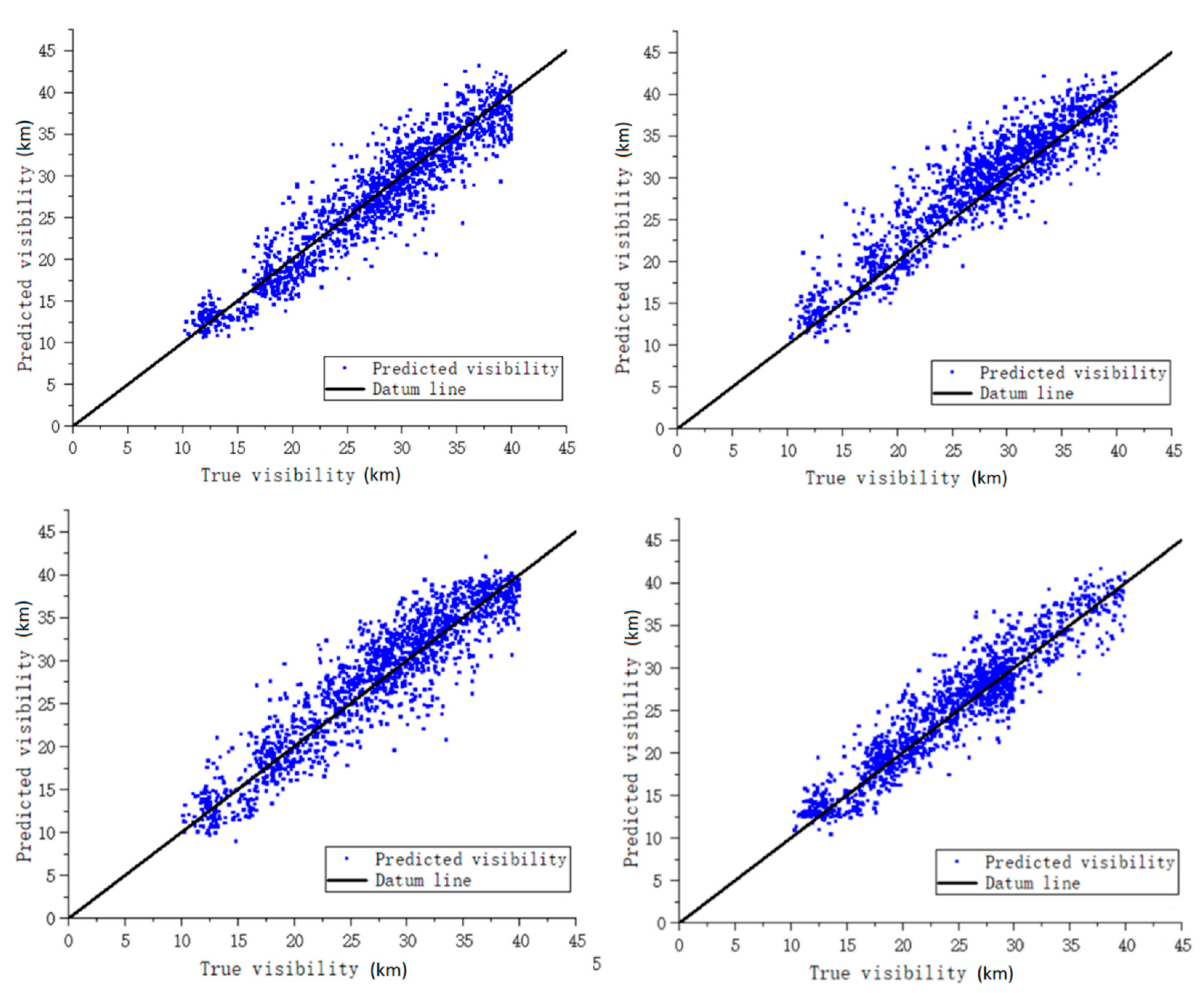
3.2.1. Comparison of Different Feature Extraction Networks
3.2.2. Performance Comparison of Different Feature Extraction Networks
4. Conclusions
Author Contributions
Funding
Institutional Review Board Statement
Informed Consent Statement
Data Availability Statement
Acknowledgments
Conflicts of Interest
References
- Khademi, S.; Rasouli, S.; Hariri, E. Measurement of the atmospheric visibility distance by imaging a linear grating with sinusoidal amplitude and having variable spatial period through the atmosphere. J. Earth Space Phys. 2016, 42, 449–458. [Google Scholar]
- Zhuang, Z.; Tai, H.; Jiang, L. Changing Baseline Lengths Method of Visibility Measurement and Evaluation. Acta Opt. Sin. 2016, 36, 0201001. [Google Scholar] [CrossRef]
- Song, H.; Chen, Y.; Gao, Y. Visibility estimation on road based on lane detection and image inflection. J. Comput. Appl. 2012, 32, 3397–3403. [Google Scholar] [CrossRef]
- Liu, N.; Ma, Y.; Wang, Y. Comparative Analysis of Atmospheric Visibility Data from the Middle Area of Liaoning Province Using Instrumental and Visual Observations. Res. Environ. Sci. 2012, 25, 1120–1125. [Google Scholar]
- Minnis, P.; Doelling, D.R.; Nguyen, L.; Miller, W.F.; Chakrapani, V. Assessment of the Visible Channel Calibrations of the VIRS on TRMM and MODIS on Aqua and Terra. J. Atmos. Ocean. Technol. 2008, 25, 385–400. [Google Scholar] [CrossRef] [Green Version]
- Chattopadhyay, P.; Ray, A.; Damarla, T. Simultaneous tracking and counting of targets in a sensor network. J. Acoust. Soc. Am. 2016, 139, 2108. [Google Scholar] [CrossRef]
- Zhang, J.; Zhang, G.Y.; Sun, G.F.; Su, S.; Zhang, J.L. Calibration Method for Standard Scattering Plate Calibration System Used in Calibrating Visibility Meter. Acta Photonica Sin. 2017, 46, 312003. [Google Scholar] [CrossRef]
- Huang, S.C.; Chen, B.H.; Wang, W.J. Visibility Restoration of Single Hazy Images Captured in Real-World Weather Conditions. IEEE Trans. Circuits Syst. Video Technol. 2014, 24, 1814–1824. [Google Scholar] [CrossRef]
- Farhan, H.; Jechang, J. Visibility Enhancement of Scene Images Degraded by Foggy Weather Conditions with Deep Neural Networks. J. Sens. 2016, 1–9. [Google Scholar] [CrossRef]
- Ling, Z.; Fan, G.; Gong, J.; Guo, S. Learning deep transmission network for efficient image dehazing. Multimed. Tools Appl. 2019, 78, 213–236. [Google Scholar] [CrossRef]
- Mingye, J.; Zhenfei, G.; Dengyin, Z.; Qin, H. Visibility Restoration for Single Hazy Image Using Dual Prior Knowledge. Math. Probl. Eng. 2017, 2017, 8190182.1–8190182.10. [Google Scholar]
- Zhu, L.; Zhu, G.D.; Han, L.; Wang, N. The Application of Deep Learning in Airport Visibility Forecast. Atmos. Clim. Sci. 2017, 7, 314–322. [Google Scholar] [CrossRef] [Green Version]
- Li, S.Y.; Fu, H.; Lo, W.L. Meteorological Visibility Evaluation on Webcam Weather Image Using Deep Learning Features. Int. J. Comput. Theory Eng. 2017, 9, 455–461. [Google Scholar] [CrossRef] [Green Version]
- Chen, B.H.; Huang, S.C.; Li, C.Y.; Kuo, S.Y. Haze Removal Using Radial Basis Function Networks for Visibility Restoration Applications. IEEE Trans. Neural Netw. Learn. Syst. 2017, 99, 1–11. [Google Scholar]
- Chaabani, H.; Werghi, N.; Kamoun, F.; Taha, B.; Outay, F.; Yasar, A.-U.-H. Estimating meteorological visibility range under foggy weather conditions: A deep learning approach. Procedia Comput. Sci. 2018, 141, 478–483. [Google Scholar] [CrossRef]
- Palvanov, A.; Cho, Y.I. DHCNN for Visibility Estimation in Foggy Weather Conditions[C]. In Proceedings of the 2018 Joint 10th International Conference on Soft Computing and Intelligent Systems (SCIS) and 19th International Symposium on Advanced Intelligent Systems (ISIS), Toyama, Japan, 5–8 December 2018. [Google Scholar]
- You, Y.; Lu, C.W.; Wang, W.M.; Tang, C.-K. Relative CNN-RNN: Learning Relative Atmospheric Visibility from Images. IEEE Trans. Image Process. 2018, 28, 45–55. [Google Scholar] [CrossRef] [PubMed]
- Choi, Y.; Choe, H.-G.; Choi, J.Y.; Kim, K.T.; Kim, J.-B.; Kim, N.-I. Automatic Sea Fog Detection and Estimation of Visibility Distance on CCTV. J. Coast. Res. 2018, 85, 881–885. [Google Scholar] [CrossRef]
- Ren, W.; Pan, J.; Zhang, H.; Cao, H.; Yang, M.-H. Single Image Dehazing via Multi-scale Convolutional Neural Networks with Holistic Edges. Int. J. Comput. Vis. 2019, 128, 240–259. [Google Scholar] [CrossRef]
- Lu, Z.; Lu, B.; Zhang, H.; Fu, Y.; Qiu, Y.; Zhan, T.; Zhenyu, L.; Bingjian, L.; Hengde, Z.; You, F.; et al. A method of visibility forecast based on hierarchical sparse representation. J. Vis. Commun. Image Represent. 2019, 58, 160–165. [Google Scholar] [CrossRef]
- Li, Q.; Tang, S.; Peng, X.; Ma, Q. A Method of Visibility Detection Based on the Transfer Learning. J. Atmos. Ocean. Technol. 2019, 36, 1945–1956. [Google Scholar] [CrossRef]
- Outay, F.; Taha, B.; Chaabani, H.; Kamoun, F.; Werghi, N.; Yasar, A.-U.-H. Estimating ambient visibility in the presence of fog: A deep convolutional neural network approach. Pers. Ubiquitous Comput. 2019, 25, 51–62. [Google Scholar] [CrossRef]
- Zhang, C.; Wu, M.; Chen, J.Y.; Chen, K.; Zhang, C.; Xie, C.; Huang, B.; He, Z. Weather Visibility Prediction Based on Multimodal Fusion. IEEE Access 2019, 7, 74776–74786. [Google Scholar] [CrossRef]
- Palvanov, A.; Cho, Y. VisNet: Deep Convolutional Neural Networks for Forecasting Atmospheric Visibility. Sensors 2019, 19, 1343. [Google Scholar] [CrossRef] [Green Version]
- Wai, L.L.; Zhu, M.M.; Fu, H. Meteorology Visibility Estimation by Using Multi-Support Vector Regression Method. J. Adv. Inf. Technol. 2020, 11, 40–47. [Google Scholar]
- Malm, W.; Cismoski, S.; Prenni, A.; Peters, M. Use of cameras for monitoring visibility impairment. Atmos. Environ. 2018, 175, 167–183. [Google Scholar] [CrossRef]
- De Bruine, M.; Krol, M.; van Noije, T.; Sager, P.L.; Röckmann, T. The impact of precipitation evaporation on the atmospheric aerosol distribution in EC-Earth v3.2.0. Geosci. Model Dev. Discuss. 2017, 11, 1–34. [Google Scholar] [CrossRef] [Green Version]
- Hautiére, N.; Tarel, J.P.; Lavenant, J.; Aubert, D. Automatic fog detection and estimation of visibility distance through use of an onboard camera. Mach. Vis. Appl. 2006, 17, 8–20. [Google Scholar] [CrossRef]
- Yang, W.; Liu, J.; Yanga, S.; Guo, Z. Scale-Free Single Image Deraining Via Visibility-Enhanced Recurrent Wavelet Learning. IEEE Trans. Image Process. 2019, 28, 2948–2961. [Google Scholar] [CrossRef]
- Cheng, X.B.; Yang, G.; Liu, T.; Olofsson, T.; Li, H. A variational approach to atmospheric visibility estimation in the weather of fog and haze. Sustain. Cities Soc. 2018, 39, 215–224. [Google Scholar] [CrossRef]
- Chaabani, H.; Kamoun, F.; Bargaoui, H.; Outay, F.; Yasar, A.-U.-H. Neural network approach to visibility range estimation under foggy weather conditions. Procedia Comput. Sci. 2017, 113, 466–471. [Google Scholar] [CrossRef]
- Li, J.; Lo, W.L.; Fu, H.; Chung, H.S.H. A Transfer Learning Method for Meteorological Visibility Estimation Based on Feature Fusion Method. Appl. Sci. 2021, 11, 997. [Google Scholar] [CrossRef]
- Simonyan, K.; Zisserman, A. Very Deep Convolution Networks for Large-scale Image Recognition. In Proceedings of the International Conference on Learning Representations, ICLR 2015, San Diego, CA, USA, 7–9 May 2015. [Google Scholar]
- He, K.; Zhang, X.; Ren, S.; Sun, J. Deep Residual Learning for Image Recognition. In Proceedings of the 2016 IEEE Conference on Computer Vision and Pattern Recognition (CVPR), Las Vegas, NV, USA, 27–30 June 2016. [Google Scholar]
- Huang, G.; Liu, Z.; Van Der Maaten, L.; Weinberger, K.Q. Densely Connected Convolutional Networks. In Proceedings of the 2017 IEEE Conference on Computer Vision and Pattern Recognition (CVPR), Honolulu, HI, USA, 21–26 July 2017. [Google Scholar]
- Hu, M.; Wu, T.; Weir, J.D. An Adaptive Particle Swarm Optimization with Multiple Adaptive Methods. IEEE Trans. Evol. Comput. 2013, 17, 705–720. [Google Scholar] [CrossRef]
- Zhan, Z.H.; Zhang, J.; Li, Y.; Chung, H.S.-H. Adaptive Particle Swarm Optimization. IEEE Trans. Syst. Man Cybern. Part B 2009, 39, 1362–1381. [Google Scholar] [CrossRef] [PubMed] [Green Version]
- Han, H.; Lu, W.; Qiao, J. An Adaptive Multi-objective Particle Swarm Optimization Based on Multiple Adaptive Methods. IEEE Trans. Cybern. 2017, 47, 2754–2767. [Google Scholar] [CrossRef] [PubMed]
- Cervante, L.; Xue, B.; Zhang, M.; Shang, L. Binary particle swarm optimisation for feature selection: A filter based approach. In Proceedings of the 2012 IEEE Congress on Evolutionary Computation, Brisbane, QLD, Australia, 10–15 June 2012. [Google Scholar]


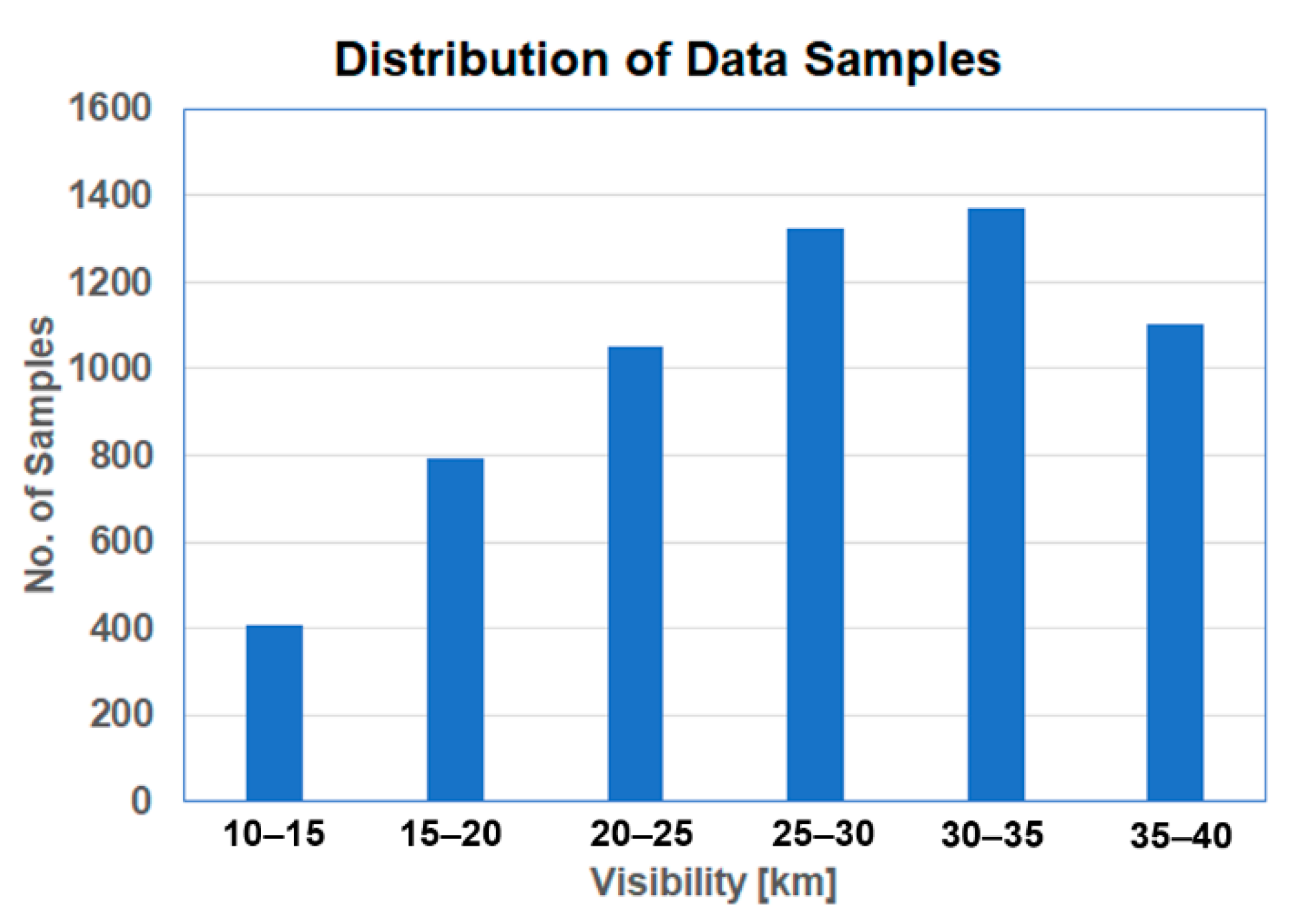
| Visibility Range (km) | ||||||
|---|---|---|---|---|---|---|
| 10–14 | 15–20 | 21–24 | 25–30 | 31–34 | 35–40 | |
| No. of training set sample images | 270 | 527 | 700 | 884 | 915 | 735 |
| No. of test set sample images | 135 | 264 | 350 | 442 | 458 | 368 |
| 405 | 791 | 1050 | 1326 | 1373 | 1103 | |
| Network | Overall Accuracy (%) |
|---|---|
| VGG-16 (%) | 90.26 → (* 90.78) |
| VGG-19 (%) | 90.32 → (* 90.85) |
| DenseNet (%) | 91.46 → (* 91.86) |
| ResNet_50 (%) | 92.72 → (* 92.23) |
| Visibility Range (km) | |||
|---|---|---|---|
| Network | 11–20 | 21–30 | 31–40 |
| VGG-16 (%) | 91.42 | 90.89 | 89.66 |
| VGG-19 (%) | 91.67 | 90.93 | 89.21 |
| DenseNet (%) | 94.34 | 93.41 | 91.23 |
| ResNet_50 (%) | 94.71 | 93.91 | 91.32 |
Publisher’s Note: MDPI stays neutral with regard to jurisdictional claims in published maps and institutional affiliations. |
© 2021 by the authors. Licensee MDPI, Basel, Switzerland. This article is an open access article distributed under the terms and conditions of the Creative Commons Attribution (CC BY) license (https://creativecommons.org/licenses/by/4.0/).
Share and Cite
Lo, W.L.; Chung, H.S.H.; Fu, H. Experimental Evaluation of PSO Based Transfer Learning Method for Meteorological Visibility Estimation. Atmosphere 2021, 12, 828. https://doi.org/10.3390/atmos12070828
Lo WL, Chung HSH, Fu H. Experimental Evaluation of PSO Based Transfer Learning Method for Meteorological Visibility Estimation. Atmosphere. 2021; 12(7):828. https://doi.org/10.3390/atmos12070828
Chicago/Turabian StyleLo, Wai Lun, Henry Shu Hung Chung, and Hong Fu. 2021. "Experimental Evaluation of PSO Based Transfer Learning Method for Meteorological Visibility Estimation" Atmosphere 12, no. 7: 828. https://doi.org/10.3390/atmos12070828
APA StyleLo, W. L., Chung, H. S. H., & Fu, H. (2021). Experimental Evaluation of PSO Based Transfer Learning Method for Meteorological Visibility Estimation. Atmosphere, 12(7), 828. https://doi.org/10.3390/atmos12070828