
Polarimetric Imaging vs. Conventional Imaging: Evaluation of Image Contrast in Fog


Abstract
:1. Introduction
2. Materials and Methods
2.1. Experimental Setup
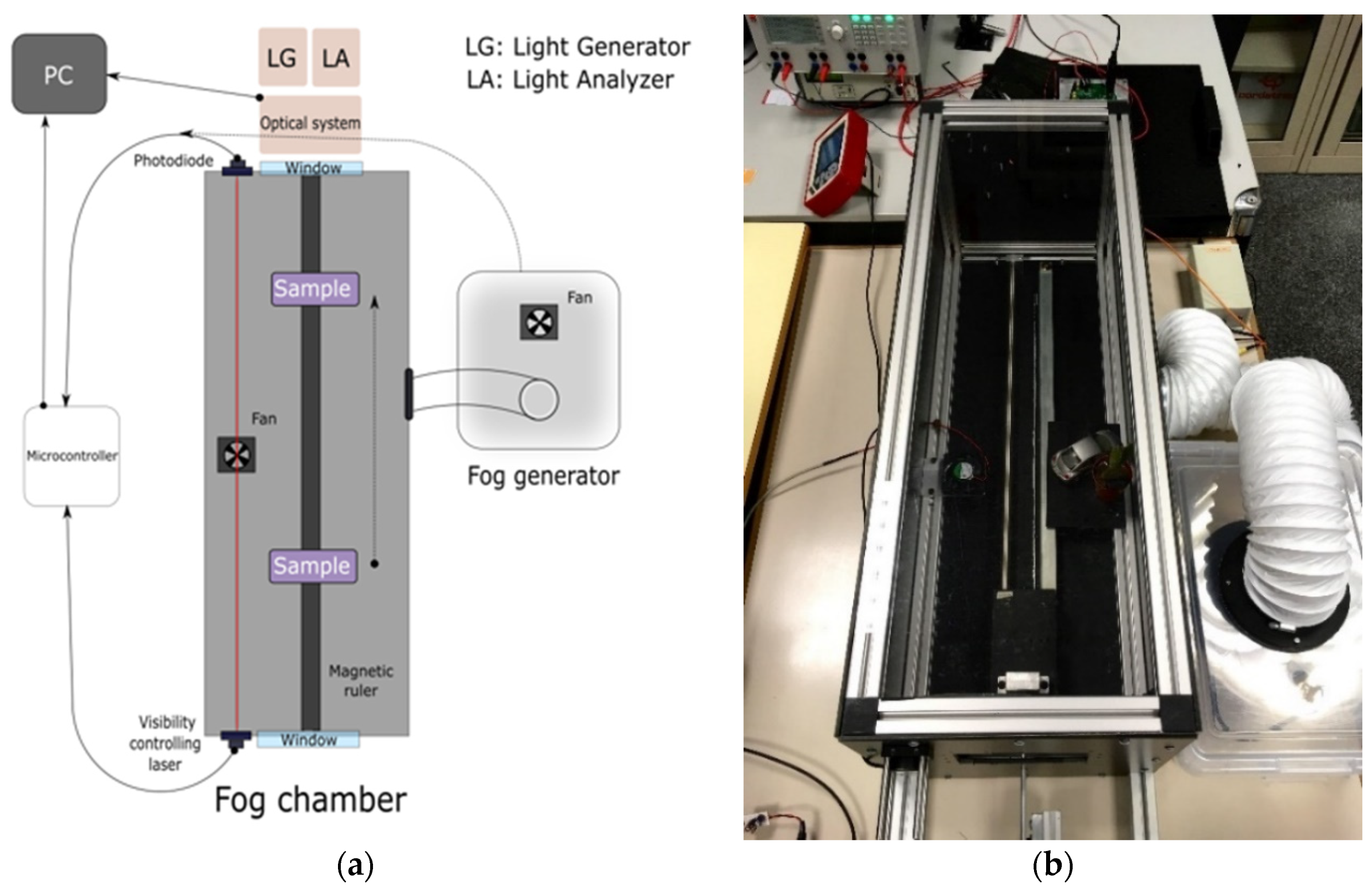
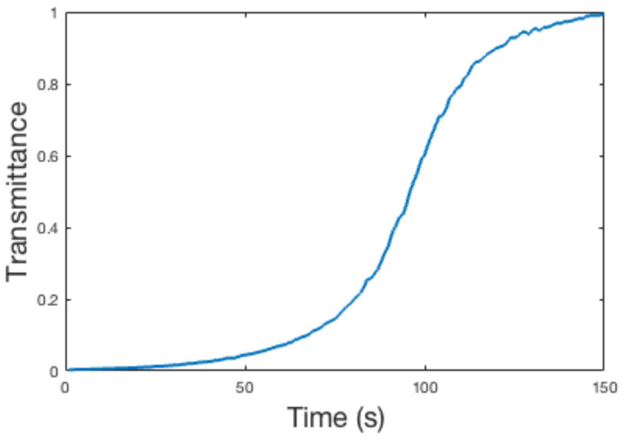
2.1.1. Fog Chamber
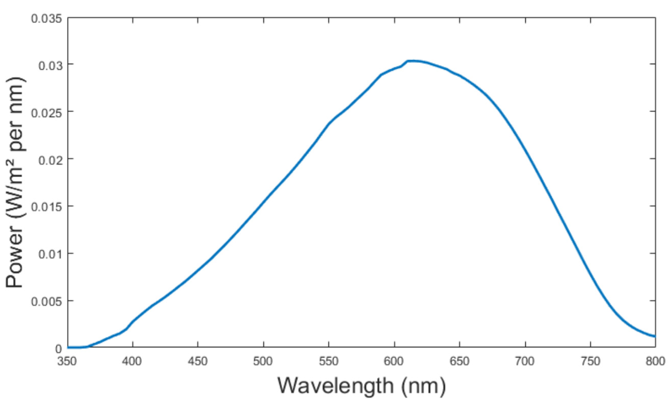
2.1.2. Illumination
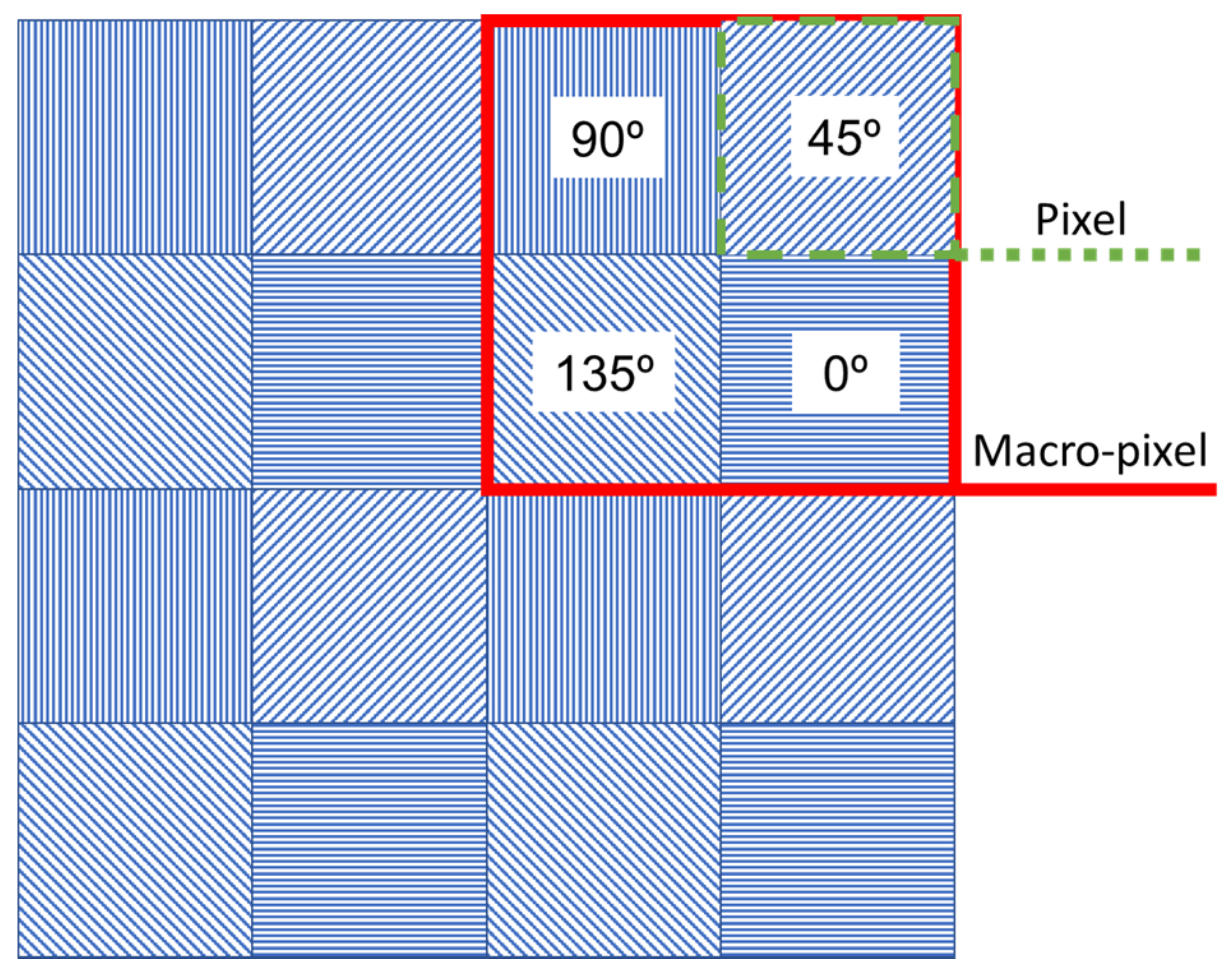
2.1.3. Detection
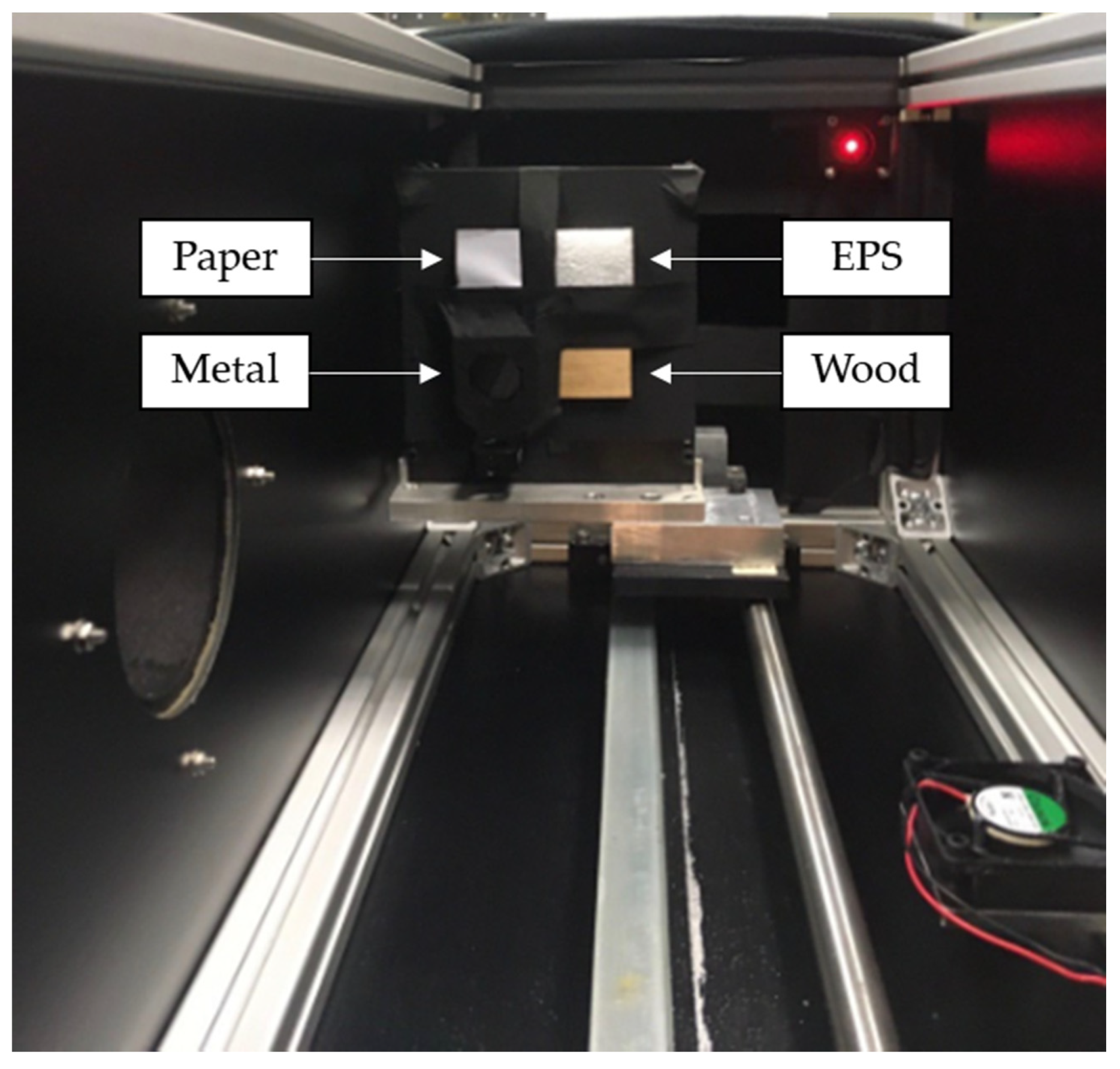
2.1.4. Samples
2.2. Image Processing
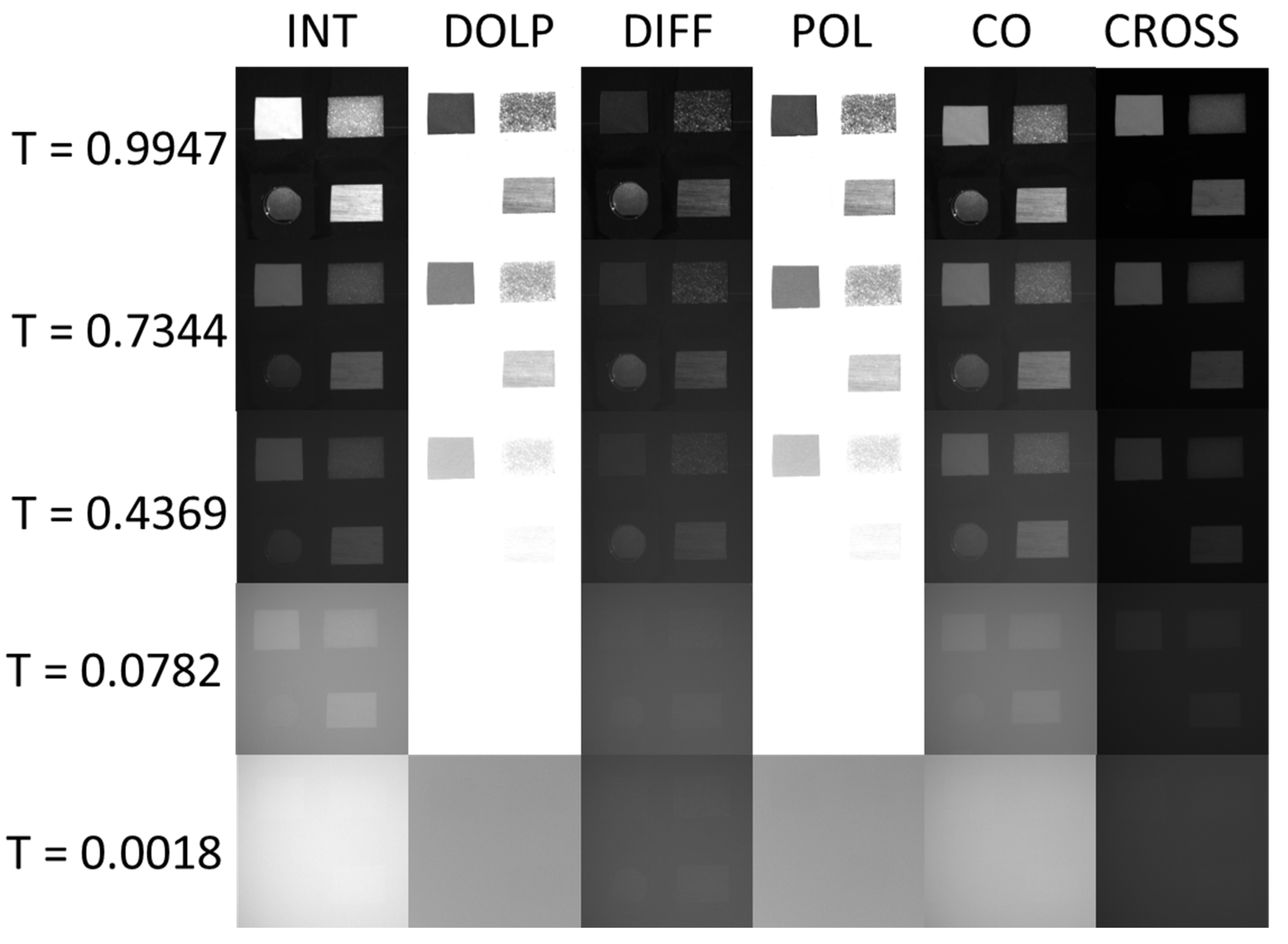
2.2.1. Imaging Modes
2.2.2. Michelson Contrast
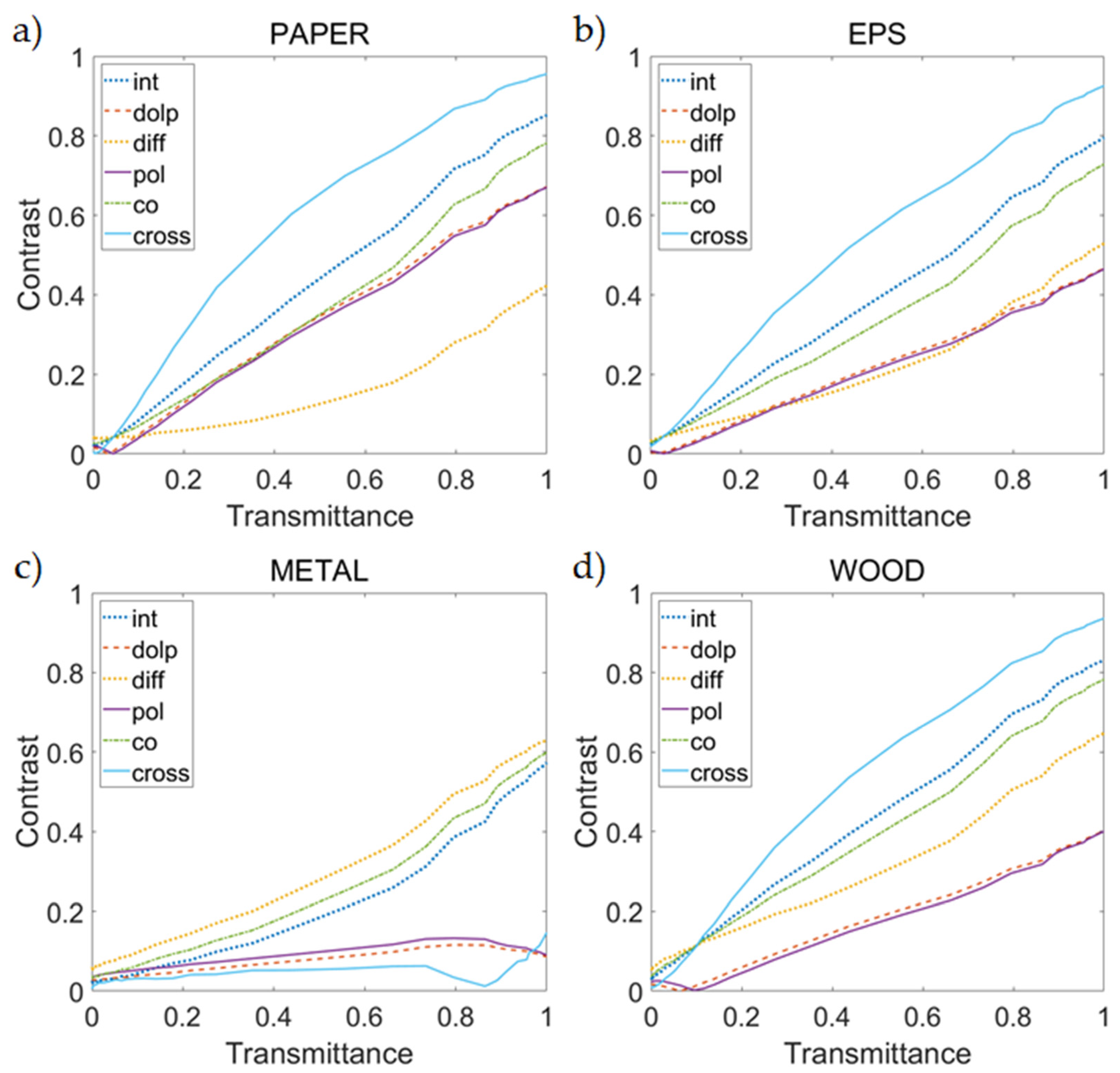
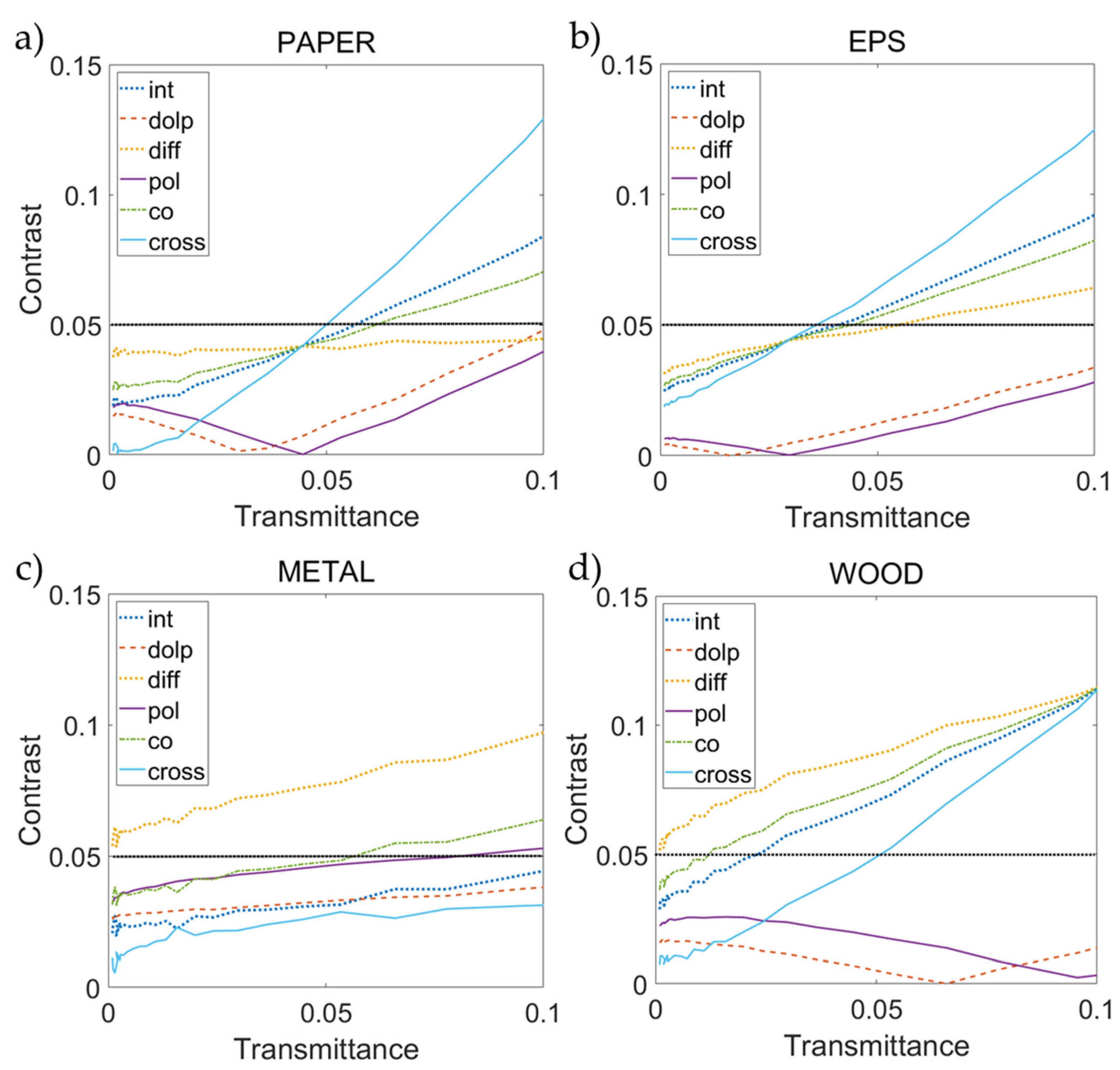
3. Results
4. Discussion
5. Conclusions
Author Contributions
Funding
Conflicts of Interest
References
- Xu, M.; Alfano, R.R. Random Walk of Polarized Light in Turbid Media. Phys. Rev. Lett. 2005, 95, 213901. [Google Scholar] [CrossRef] [PubMed]
- MacKintosh, F.; Zhu, J.X.; Pine, D.J.; Weitz, D.A. Polarization memory of multiply scattered light. Phys. Rev. B 1989, 40, 9342–9345. [Google Scholar] [CrossRef]
- Van Der Laan, J.D.; Wright, J.B.; Scrymgeour, D.A.; Kemme, S.A.; Dereniak, E.L. Evolution of circular and linear polarization in scattering environments. Opt. Express 2015, 23, 31874–31888. [Google Scholar] [CrossRef] [PubMed]
- Lewis, G.D.; Jordan, D.L.; Roberts, P.J. Backscattering target detection in a turbid medium by polarization discrimination. Appl. Opt. 1999, 38, 3937–3944. [Google Scholar] [CrossRef]
- Kartazayeva, S.A.; Ni, X.; Alfano, R.R. Backscattering target detection in a turbid medium by use of circularly and linearly polarized light. Opt. Lett. 2005, 30, 1168–1170. [Google Scholar] [CrossRef]
- Walker, J.G.; Chang, P.C.Y.; Hopcraft, K.I. Visibility depth improvement in active polarization imaging in scattering media. Appl. Opt. 2000, 39, 4933–4941. [Google Scholar] [CrossRef]
- Goudail, F.; Tyo, J.S. When is polarimetric imaging preferable to intensity imaging for target detection? J. Opt. Soc. Am. A 2010, 28, 46–53. [Google Scholar] [CrossRef] [PubMed]
- Rozé, C.; Maheu, B.; Gréhan, G.; Menard, J. Evaluations of the sighting distance in a foggy atmosphere by monte carlo simulation. Atmos. Environ. 1994, 28, 769–775. [Google Scholar] [CrossRef]
- Judd, K.M.; Thornton, M.P.; Richards, A.A. Automotive sensing: Assessing the impact of fog on LWIR, MWIR, SWIR, visible, and lidar performance. Infrared Technol. Appl. XLV 2019, 11002, 110021F. [Google Scholar] [CrossRef]
- Schechner, Y.Y.; Narasimhan, S.G.; Nayar, S.K. Polarization-based vision through haze. Appl. Opt. 2003, 42, 511–525. [Google Scholar] [CrossRef] [PubMed]
- Rowe, M.P.; Pugh, E.N.; Tyo, J.S.; Engheta, N. Polarization-difference imaging: A biologically inspired technique for observation through scattering media. Opt. Lett. 1995, 20, 608–610. [Google Scholar] [CrossRef]
- Tremblay, G.; Roy, G. Study of polarization memory’s impact on detection range in natural water fogs. Appl. Opt. 2020, 59, 1885–1895. [Google Scholar] [CrossRef]
- Fade, J.; Panigrahi, S.; Carré, A.; Frein, L.; Hamel, C.; Bretenaker, F.; Ramachandran, H.; Alouini, M. Long-range polarimetric imaging through fog. Appl. Opt. 2014, 53, 3854–3865. [Google Scholar] [CrossRef] [PubMed] [Green Version]
- Blin, R.; Ainouz, S.; Canu, S.; Meriaudeau, F. Road scenes analysis in adverse weather conditions by polarization-encoded images and adapted deep learning. In Proceedings of the 2019 IEEE Intelligent Transportation Systems Conference (ITSC), Auckland, New Zealand, 27–30 October 2019; pp. 27–32. [Google Scholar]
- Blin, R.; Ainouz, S.; Canu, S.; Meriaudeau, F. A new multimodal RGB and polarimetric image dataset for road scenes analysis. In Proceedings of the 2020 IEEE/CVF Conference on Computer Vision and Pattern Recognition Workshops (CVPRW), Seattle, WA, USA, 14–19 June 2020; Volume 1, pp. 867–876. [Google Scholar]
- Chipman, R.A. Polarimetry. In Handbook of Optics; Van Stryland, E.W., Williams, D.R., Wolfe, W.L., Eds.; McGraw-Hill: New York, NY, USA, 1995; Volume 2, pp. 22.1–22.37. [Google Scholar]
- Nothdurft, R.E.; Yao, G. Effects of turbid media optical properties on object visibility in subsurface polarization imaging. Appl. Opt. 2006, 45, 5532–5541. [Google Scholar] [CrossRef] [PubMed] [Green Version]
- Novikova, T.; Beniere, A.; Goudail, F.; De Martino, A. Contrast evaluation of the polarimetric images of different targets in turbid medium: Possible sources of systematic errors. SPIE Def. Secur. Sens. 2010, 7672, 76720Q. [Google Scholar] [CrossRef]
- Nothdurft, R.; Yao, G. Expression of target optical properties in subsurface polarization-gated imaging. Opt. Express 2005, 13, 4185–4195. [Google Scholar] [CrossRef] [PubMed] [Green Version]
- Vannier, N.; Goudail, F.; Plassart, C.; Boffety, M.; Feneyrou, P.; Leviandier, L.; Galland, F.; Bertaux, N. Comparison of different active polarimetric imaging modes for target detection in outdoor environment. Appl. Opt. 2016, 55, 2881–2891. [Google Scholar] [CrossRef]
- Rodes, C.; Smith, T.; Crouse, R.; Ramachandran, G. Measurements of the Size Distribution of Aerosols Produced by Ultrasonic Humidification. Aerosol Sci. Technol. 1990, 13, 220–229. [Google Scholar] [CrossRef] [Green Version]
- Kooij, S.; Astefanei, A.; Corthals, G.L.; Bonn, D. Size distributions of droplets produced by ultrasonic nebulizers. Sci. Rep. 2019, 9, 6128. [Google Scholar] [CrossRef]
- Satat, G.; Tancik, M.; Raskar, R. Towards photography through realistic fog. In Proceedings of the 2018 IEEE International Conference on Computational Photography (ICCP), Pittsburgh, PA, USA, 4–6 May 2018; pp. 1–10. [Google Scholar]
- Hickman, D.L.; Smith, M.I.; Kim, K.S.; Choi, H.-J. Polarimetric imaging: System architectures and trade-offs. In Electro-Optical and Infrared Systems: Technology and Applications XV; SPIE-Intl Soc Optical Eng: Bellingham, WA, USA, 2018; Volume 10795, p. 107950B. [Google Scholar]
- Peli, E. Contrast in complex images. J. Opt. Soc. Am. A 1990, 7, 2032–2040. [Google Scholar] [CrossRef]
- Bex, P.J.; Makous, W. Spatial frequency, phase, and the contrast of natural images. J. Opt. Soc. Am. A 2002, 19, 1096–1106. [Google Scholar] [CrossRef] [PubMed] [Green Version]
- Dumont, E.; Cavallo, V. Extended Photometric Model of Fog Effects on Road Vision. Transp. Res. Rec. J. Transp. Res. Board 2004, 1862, 77–81. [Google Scholar] [CrossRef]
- Kim, M.; Keller, D.; Bustamante, C. Differential polarization imaging. I. Theory. Biophys. J. 1987, 52, 911–927. [Google Scholar] [CrossRef] [Green Version]

| Name | Measurements |
|---|---|
| Horizontal linear polarizer () | |
| Vertical linear polarizer () | |
| linear polarizer | |
| linear polarizer | |
| Left circular polarizer | |
| Right circular polarizer |
| Parameter | Mean Value | Standard Deviation |
|---|---|---|
| Azimuth angle | −0.64 () | 0.19 |
| Ellipticity | −0.91 () | 0.29 |
| Degree of polarization | 99.93 (%) | 0.29 |
| Degree of linear polarization | 99.88 (%) | 0.27 |
| Material | DOLP |
|---|---|
| Paper | 0.11 |
| EPS | 0.27 |
| Metal | 0.89 |
| Wood | 0.30 |
| Background | 0.75 |
| Image Mode Name | Abbreviation | Computation |
|---|---|---|
| Intensity/Stokes 0 | ||
| Stokes 1 | ||
| Stokes 2 | ||
| Co-polarized | ||
| Cross-polarized | ||
| Degree of linear polarization | ||
| Differential polarization | ||
| Degree of co-polarization |
Publisher’s Note: MDPI stays neutral with regard to jurisdictional claims in published maps and institutional affiliations. |
© 2021 by the authors. Licensee MDPI, Basel, Switzerland. This article is an open access article distributed under the terms and conditions of the Creative Commons Attribution (CC BY) license (https://creativecommons.org/licenses/by/4.0/).
Share and Cite
Ballesta-Garcia, M.; Peña-Gutiérrez, S.; Val-Martí, A.; Royo, S. Polarimetric Imaging vs. Conventional Imaging: Evaluation of Image Contrast in Fog. Atmosphere 2021, 12, 813. https://doi.org/10.3390/atmos12070813
Ballesta-Garcia M, Peña-Gutiérrez S, Val-Martí A, Royo S. Polarimetric Imaging vs. Conventional Imaging: Evaluation of Image Contrast in Fog. Atmosphere. 2021; 12(7):813. https://doi.org/10.3390/atmos12070813
Chicago/Turabian StyleBallesta-Garcia, Maria, Sara Peña-Gutiérrez, Aina Val-Martí, and Santiago Royo. 2021. "Polarimetric Imaging vs. Conventional Imaging: Evaluation of Image Contrast in Fog" Atmosphere 12, no. 7: 813. https://doi.org/10.3390/atmos12070813
APA StyleBallesta-Garcia, M., Peña-Gutiérrez, S., Val-Martí, A., & Royo, S. (2021). Polarimetric Imaging vs. Conventional Imaging: Evaluation of Image Contrast in Fog. Atmosphere, 12(7), 813. https://doi.org/10.3390/atmos12070813