Single Image Dehazing Using Sparse Contextual Representation

Abstract

In this paper, we propose a novel method to remove haze from a single hazy input image based on the sparse representation. In our method, the sparse representation is proposed to be used as a contextual regularization tool, which can reduce the block artifacts and halos produced by only using dark channel prior without soft matting as the transmission is not always constant in a local patch. A novel way to use dictionary is proposed to smooth an image and generate the sharp dehazed result. Experimental results demonstrate that our proposed method performs favorably against the state-of-the-art dehazing methods and produces high-quality dehazed and vivid color results.

1. Introduction

Natural images captured outdoors are often degraded by bad weather [1], which greatly reduces the quality of captured images. Figure 1 shows an example of hazy images—the hazy input loses some color and contrast information, which makes it hard to distinguish the distant objects from the hazy image. The reason for this phenomena is that the degradation is spatially variant [1].

Haze removal or image dehazing is urgently needed in computer vision applications. First of all, removing fog from a hazy image can significantly improve the visibility in the image and greatly rectify the color shift caused by the air-light. In addition, the quality of the images will affect the results of the related computer vision algorithms to some extent, from the low-level image analysis (e.g., edge detection or line segmentation) to the high-level image understanding (e.g., object detection or scene parsing).

However, image dehazing is an ill-posed problem as the physical formulation has at least four unknowns per pixel and only three equations. To solve this problem, numerous single image dehazing approaches have been proposed by using multiple inputs [2,3] or sharp image priors [1,4,5]. Fattal [4] proposed removing haze by explaining an image via a model that accounts for the surface shading and the scene transmission. The assumption that the surface shading and the medium transmission functions are locally statistically uncorrelated solved a constant albedo and the atmospheric-albedo ambiguity to generate haze-free images. However, it cannot process heavily hazy images and grayscale images well. He et al. [1] proposed the dark channel’s statistical observation known as dark channel prior (DCP). With this prior, He at el. estimated the thickness of fog locally from the dark-channel pixels within a local patch. However, it should be noted that the images, as well as the haze, could be affected by uncertainties and inaccuracies. Therefore, the need arises to pre-treat images with soft computing techniques based on fuzzy logic [6,7]. Gibson and Nguyen [8] proposed an improved DCP for haze removal from the input. Unlike the DCP in [1], Gibson and Nguyen [8] proposed an improved DCP by assuming a zero minimal value, which improves DCP searches for the darkest pixel average inside of each ellipsoid. Fattal [9] proposed another haze removal method based on the characteristic of small image patches, which form a line in a small image patch of the RGB color space. Based on this distribution, Fattal [9] proposed a color-lines model and recovered the scene by considering the color-lines’ offset from the sharp image. Zhu et al. [10] proposed a color attenuation prior (CAP) according to sharp image statistics. They introduced a linear model for the fog image’s scene depth with the CAP to compute the parameters of the linear model by a supervised learning approach. Li and Zheng [11] decomposed the hazy input’s dark channel into two layers (i.e., a detail layer and a base layer) based on edge-preserving decomposition. Then, the base layer was used to estimate the transmission map for haze removal.

In addition to image priors-based methods, another line of research tries to remove haze based on multi-image fusion. Ancuti et al. [12,13] illustrated the effectiveness of fusion-based methods for removing haze from a single input image. In [13], two original hazy inputs are first pre-processed by contrast enhancing and white balance. Then, these two derived inputs are blended to generate the dehazed result by computing three weight maps. To remove some halo artifacts, this method employs a multiscale scheme to produce dehazed results.

Following these existing methods, we further develop a new dehazing method based on a sparse contextual representation. Sparse representation has been commonly used for image denoising, super-resolution, deblurring, and other restoration tasks [14,15]. In this work, we propose a new sparse contextual representation to reduce the halo and block artifacts in the image dehazing task. Our proposed method is based on two observations. The first one is that the depth or transmission map keeps the main structure of the original input image. Another one is that the depth or transmission map is locally smooth. Therefore, we use the sparse representation to smooth the boundary-constrained map. In the proposed method, we obtain two different transmission maps—one of them provides the main structure while the other retains the image details. We fuse these two transmission maps using the sparse contextual representation and obtain the refined transmission map. Figure 2 illustrates an example of our proposed algorithm using sparse representation, from which we observe that our proposed method can recover a smooth transmission map and generate a high-quality haze-free image.

2. Hazy Image Formulation

The commonly used hazy image model is presented in [16] as

$$\mathbf{I}\left(\mathbf{x}\right)=t\left(\mathbf{x}\right)\mathbf{J}\left(\mathbf{x}\right)+(1-t(\mathbf{x}\left)\right)\mathbf{A},$$

(1)

where the vectors $\mathbf{I}\left(\mathbf{x}\right)$ and $\mathbf{J}\left(\mathbf{x}\right)$ denote the intensities for the three RGB channels of the pixel at $\mathbf{x}$ of the observed hazy input and the corresponding haze-free image, respectively, $\mathbf{A}$ is the atmospheric light of the hazy input. In addition, t is the transmission map, which defines the probability of the light reaching the camera sensor from the object, x is the position of a pixel in image. Recovering a haze-free image $\mathbf{J}$ from the observed haze image $\mathbf{I}$ is equal to solve for the $\mathbf{A}$ and the t from the $\mathbf{I}$. The two terms $\mathbf{J}\left(\mathbf{x}\right)t\left(\mathbf{x}\right)$ and $(1-t(\mathbf{x}\left)\right)\mathbf{A}$ in Equation (1) are regarded as direct attenuation and the contribution of the air light $\mathbf{A}$, respectively.

3. Our Method

In this paper, we propose a novel method to estimate the transmission map using sparse representation. We employ the sparse representation to fuse the multiscale transmission maps. Firstly, we obtain the pixel-wise and patch-wise transmission maps. Secondly, we obtain the structure from the patch-wise transmission map and details from the pixel-wise one via sparse representation. Finally, we add the details to its structure, which produces the final transmission map.

3.1. Piecewise-Smooth Assumption

As indicated in [1], only using dark channel prior without soft matting would generate some halos and block artifacts in dehazing as the transmission coefficients are not always constant in a local patch. To address this problem, we assume that the pixels in the same object share similar transmission coefficients. This assumption is widely adopted [5,9]. Fattal [9] expected that the scene depth existing in an image would be piece-wise-smooth, which in turn leads to smooth scattering coefficients. This assumption implies that the resulting transmission coefficients ${\left\{t\left(\mathbf{x}\right)\right\}}_{\mathbf{x}\in \mathbf{I}}$ are also piece-wise smoothed in the whole scene and are smooth at neighboring pixels in some local region corresponding to the same object. Based on this assumption, we propose a new sparse contextual representation network for haze removal in this paper.

3.2. The Lower Bound of Transmission Map

To yield an initial transmission map of a hazy input, we can reformulate (1) as:

$$\mathbf{J}\left(\mathbf{x}\right)=\frac{\mathbf{I}\left(\mathbf{x}\right)-(1-t(\mathbf{x}\left)\right)\mathbf{A}}{max(t\left(\mathbf{x}\right),t_0)},$$

(2)

which implies that we can produce a dehazed image from a hazy input based on $\mathbf{A}$ and t, a typical value of $t_0$ is 0.1, as shown in [1]. To facilitate the calculation, we normalize the intensities of the hazy input in the RGB color space and obtain

$$t_1\left(\mathbf{x}\right)\ge \frac{{\mathbf{I}}^c\left(\mathbf{x}\right)-{\mathbf{A}}^c}{1-{\mathbf{A}}^c}\mathrm{and}{t}_2\left(\mathbf{x}\right)\ge 1-\frac{{\mathbf{I}}^c\left(\mathbf{x}\right)}{{\mathbf{A}}^c},$$

(3)

where ‘c’ is the channel index in the color space. Then, the minimum transmission can be written as:

$${\widehat{t}}_1\left(\mathbf{x}\right)=max\left(\frac{{\mathbf{I}}^r\left(\mathbf{x}\right)-{\mathbf{A}}^r}{1-{\mathbf{A}}^r},\frac{{\mathbf{I}}^g\left(\mathbf{x}\right)-{\mathbf{A}}^g}{1-{\mathbf{A}}^g},\frac{{\mathbf{I}}^b\left(\mathbf{x}\right)-{\mathbf{A}}^b}{1-{\mathbf{A}}^b}\right)$$

(4)

$${\widehat{t}}_2\left(\mathbf{x}\right)=max\left(1-\frac{{\mathbf{I}}^r\left(\mathbf{x}\right)}{{\mathbf{A}}^r},1-\frac{{\mathbf{I}}^g\left(\mathbf{x}\right)}{{\mathbf{A}}^g},1-\frac{{\mathbf{I}}^b\left(\mathbf{x}\right)}{{\mathbf{A}}^b}\right).$$

(5)

From (4) and (5), we can obtain the lower bound of the transmission map as:

$$t_b\left(\mathbf{x}\right)=max\left({\widehat{t}}_1\left(\mathbf{x}\right),{\widehat{t}}_2\left(\mathbf{x}\right)\right).$$

(6)

Equation (6) can be regarded as a special case of the lower bound of the transmission map [17] with the parameters $C_0=0$ and $C_1=255$:

$$t_b\left(\mathbf{x}\right)=min\left(max\left(\frac{{\mathbf{A}}^c-{\mathbf{I}}^c\left(\mathbf{x}\right)}{{\mathbf{A}}^c-C_0},\frac{{\mathbf{A}}^c-{\mathbf{I}}^c\left(\mathbf{x}\right)}{{\mathbf{A}}^c-C_1}\right),1\right).$$

(7)

According to our proposed piece-wise smooth assumption, we apply the maximum-minimum filter (7) on the lower bounds of the transmission coefficients for all the pixels in an image to generate a patch-wise transmission as:

$$\tilde{t}\left(\mathbf{x}\right)=\underset{\mathbf{y}\in \mathcal{N}\left(\mathbf{x}\right)}{min}\underset{\mathbf{z}\in \mathcal{N}\left(\mathbf{y}\right)}{max}{t}_b\left(\mathbf{z}\right),$$

(8)

where $\mathcal{N}$ denotes the local patch centered at a point.

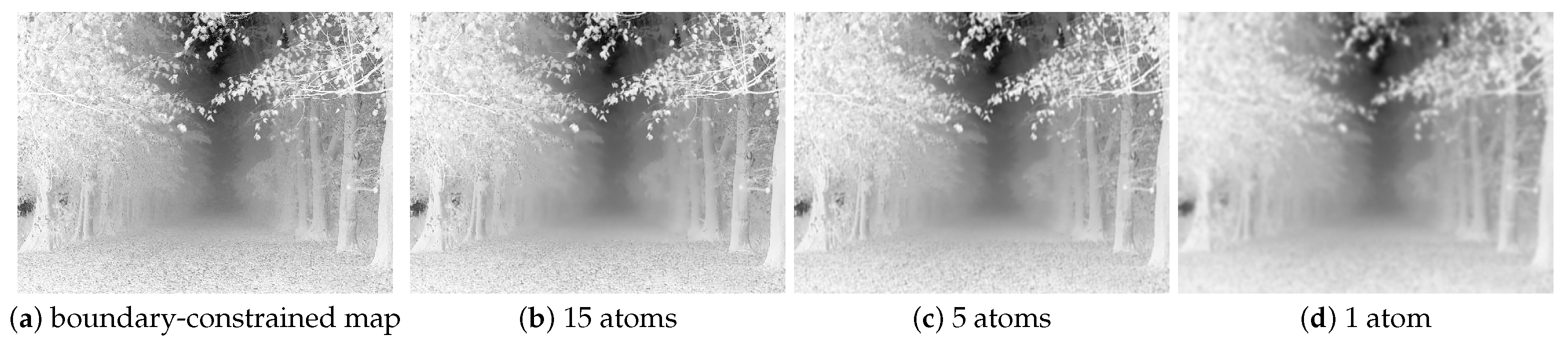
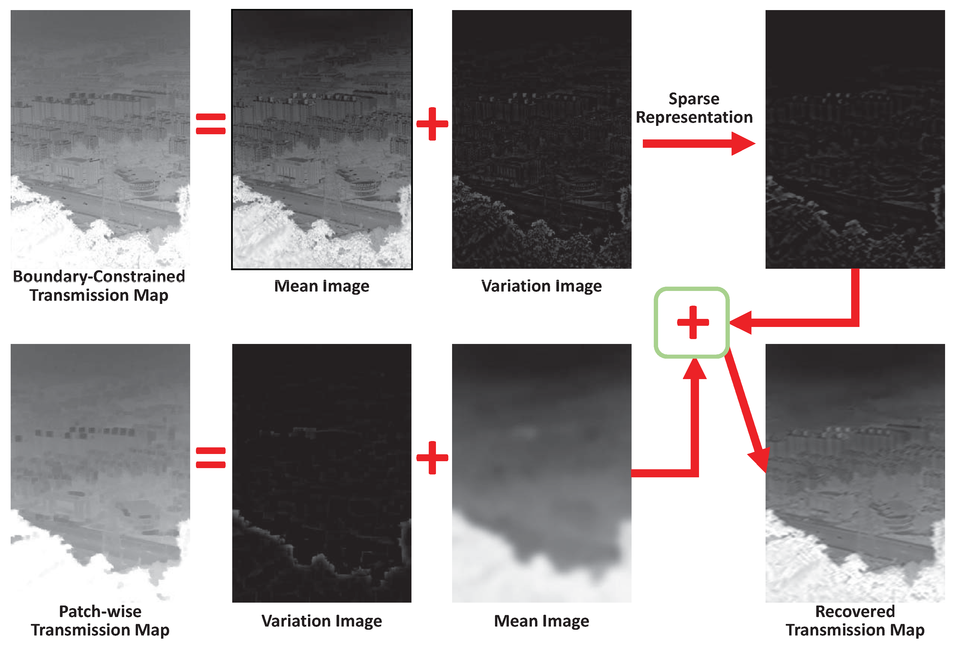
3.3. Contextual Regularization Using Sparse Representation

To smooth an image, we propose to use sparse representation to obtain a smooth transmission map. First we define an under-complete dictionary $\mathbf{D}\in {\mathbf{R}}^{n\times K}$ with K atoms ($K<n$). We learn such a dictionary from the original image. Figure 3 illustrates some smooth results on a boundary-constrained transmission map consisting of the lower bounds of transmission coefficients with a $10\times 10$ patch and 1 atom, 5 atoms and 15 atoms, respectively. From Figure 3, we can observe that the details are gradually lack in the local regions with the reduction of the number of the used atoms. In Figure 3d, only the main structure was maintained. In this paper, we use 5 atoms to construct the dictionary.

In our problem, we have input images—one is from the lower bounds ${\left\{t_b\left(\mathbf{x}\right)\right\}}_{x\in \mathbf{I}}$ of transmission coefficients, which is called as the boundary-constrained transmission map and another one is from the filtered image ${\left\{\tilde{t}\left(\mathbf{x}\right)\right\}}_{x\in \mathbf{I}}$ by using the maximum–minimum filter on the boundary-constrained map. In this case, our problem can be regarded as an inverse problem of image super resolution, which is different from image denoising, which uses only one single input by considering the noise as white Gaussian noise.

In this paper, we propose the sparse contextual representation to predict the final transmission map. According to [9], we find that the final transmission map loses a lot of local details of the original image. Thus, we can use an under-complete dictionary to represent the transmission map, which will maintain the main structure of the image but lose some local details. Figure 4 shows the whole framework recovering the transmission map using sparse representation. First we apply a mean subtraction on the boundary-constrained transmission map to get a variation image, which accounts for the local details in the transmission map. This variation image is further smoothed using sparse representation as described above. To keep the main structure of the original input image in the final transmission map, we apply a mean filter (3 × 3) on the patch-wise transmission map to get a mean image, which keeps the main structure. Finally, we recover the final transmission map by adding this mean image and the smoothed variation image, as shown in Figure 4. In this way, the final transmission map can maintain the main structure of the original image and lose a lot of local details due to the sparse-representation-based smooth operation.

3.4. Atmospheric Light Estimation

To estimate the atmospheric light [1], we first estimate the dark channel of a hazy input. Then we select the top $0.1\%$ pixels in the dark channel and choose the brightest pixel from these pixels as the final atmospheric light. Based on the estimated atmospheric light and the recovered transmission map, the final dehazed image can be produced from an input hazy image $\mathbf{I}$ using Equation (2).

4. Experimental Results

To evaluate the effectiveness of the proposed dehazing method, we compared our algorithm with some state-of-the-art methods. The patch size of $50\times 50$ with 35 atoms was used in Figure 2 and the patch size of $20\times 20$ with 25 atoms for the learned dictionary in all the experiments.

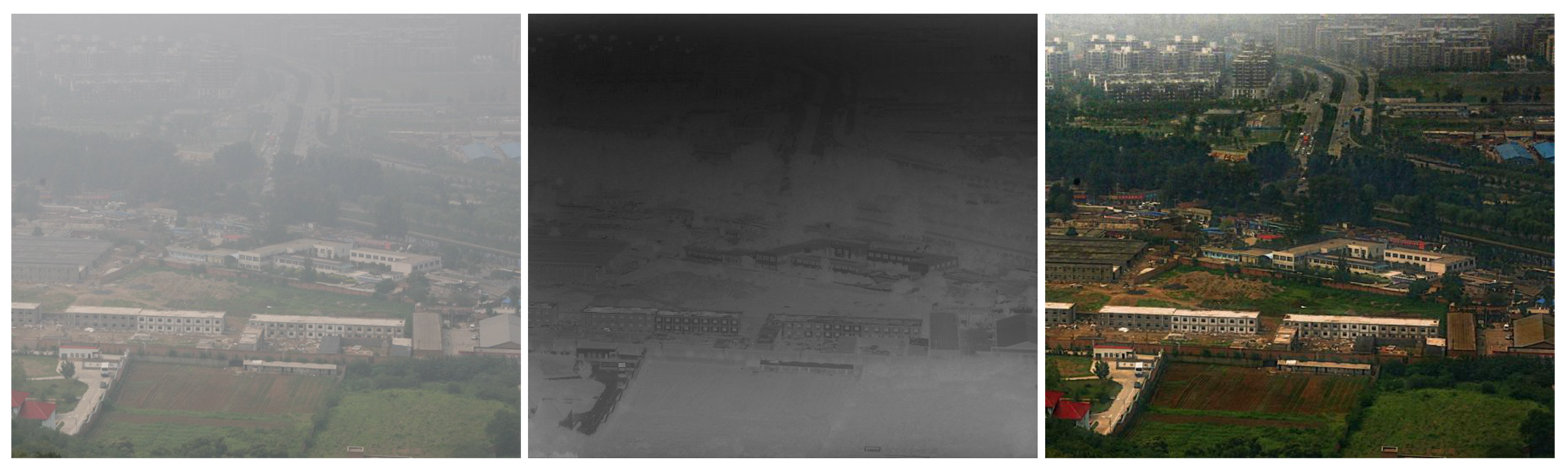
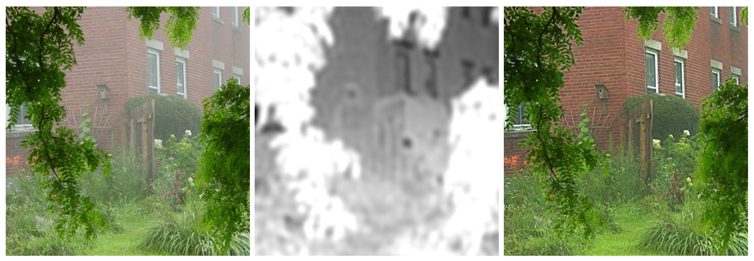
4.1. Tests on Real-World Images

In this section we show some results on several typical examples using the proposed algorithm. Figure 1 and Figure 2 show the recovered transmission maps and the dehazed images by using our method on a short-range natural outdoor image and a large-range one, respectively. The satisfied results were generated. In addition, the fog in the image of “Tiananmen” is inhomogeneous, as it often happens in real cases. Therefore, we also show that our proposed algorithm is able to remove inhomogeneous fog in Figure 5. Then, we show three dehazed examples with homogeneous fog in Figure 6. From Figure 5 and Figure 6, we can observe that the recovered transmission maps from different haze images are realistic, which is coherent with human perception.

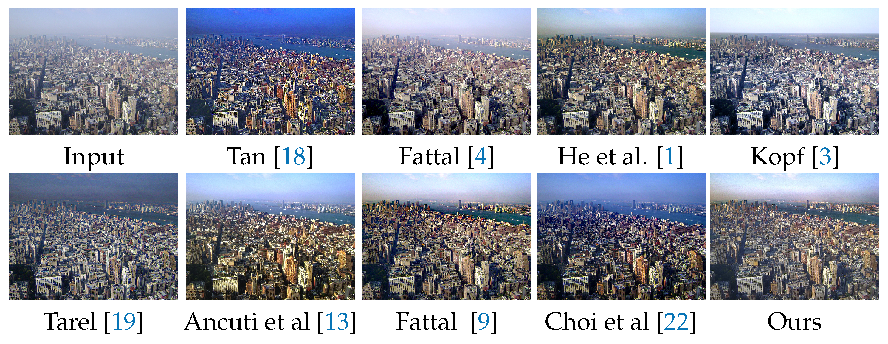
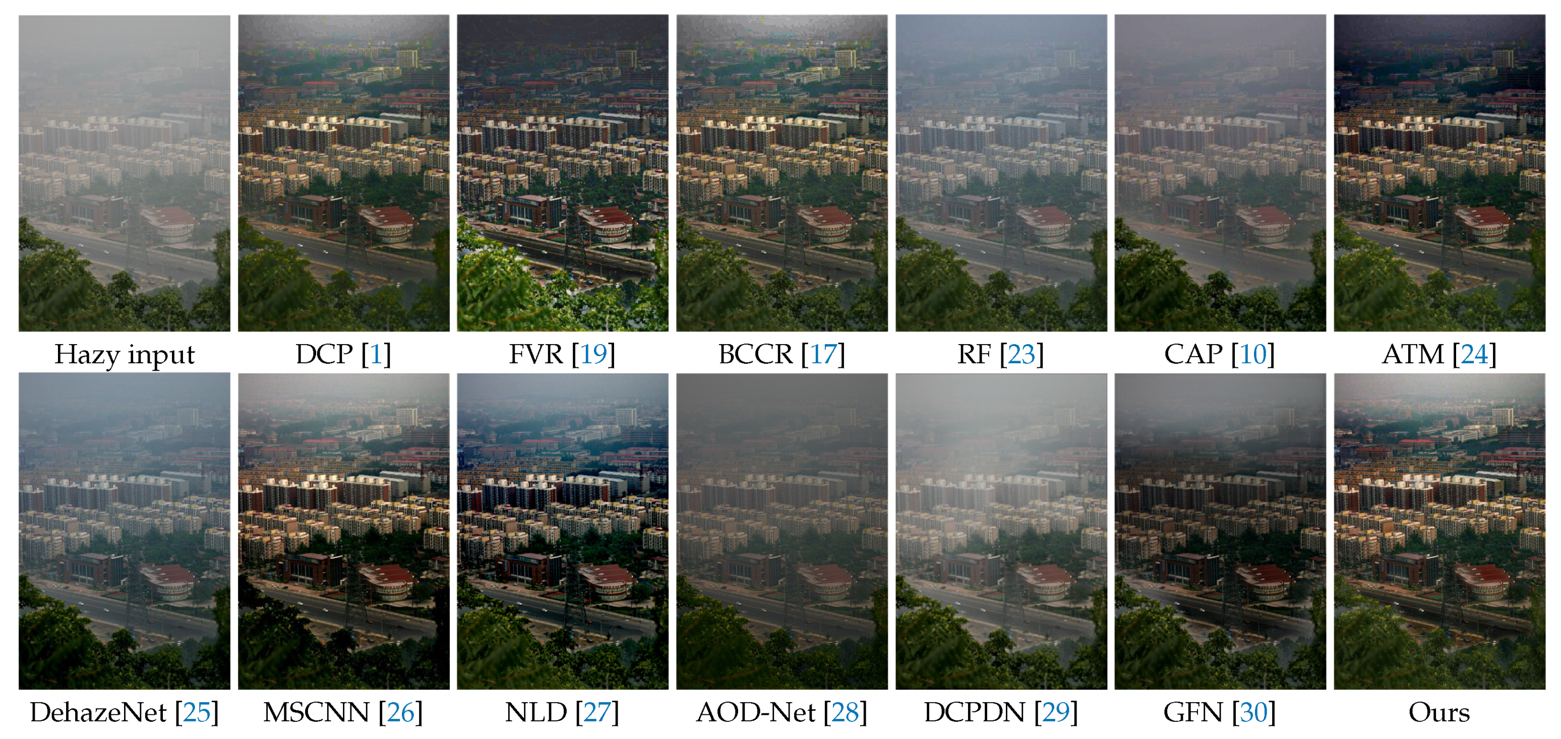
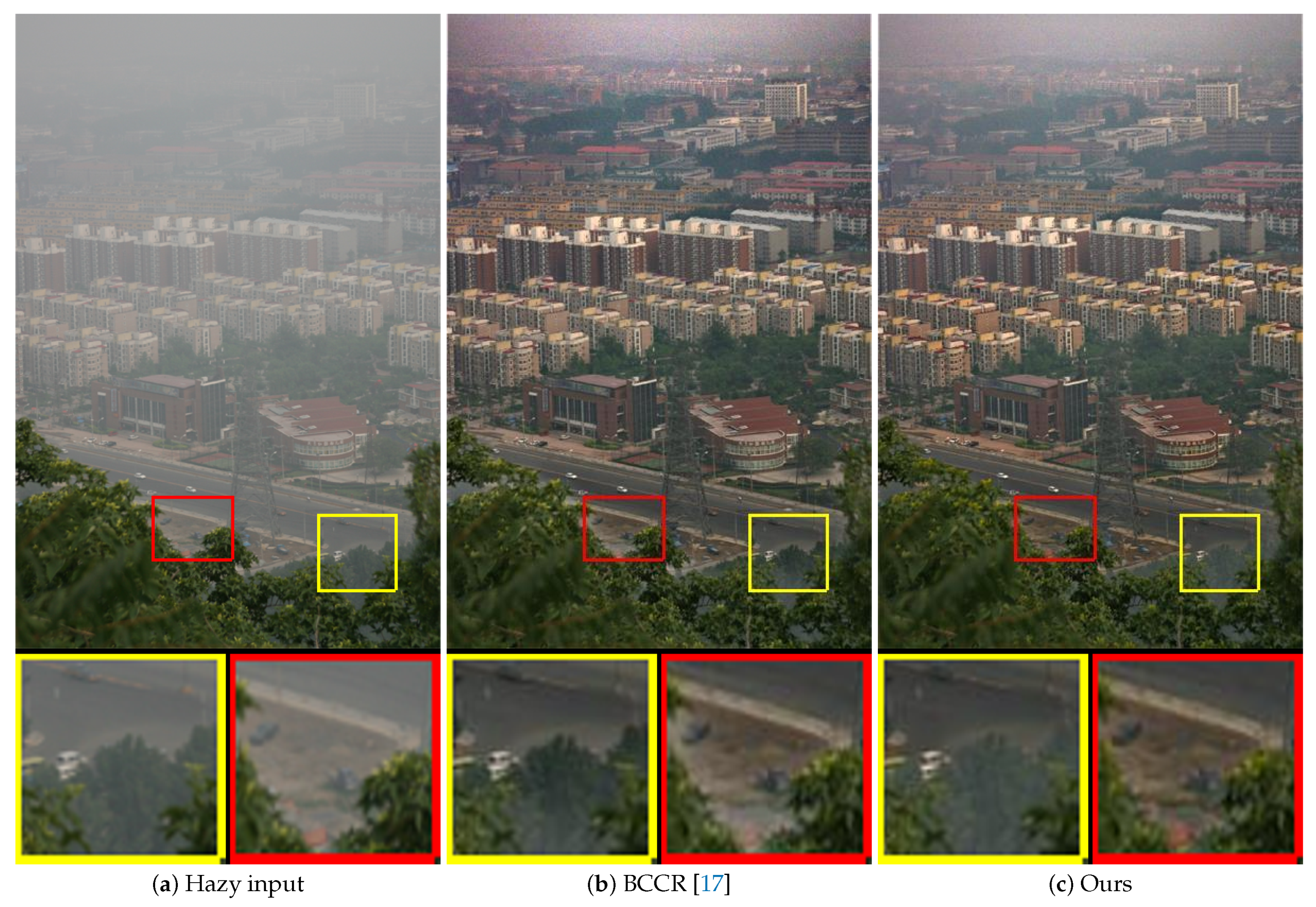
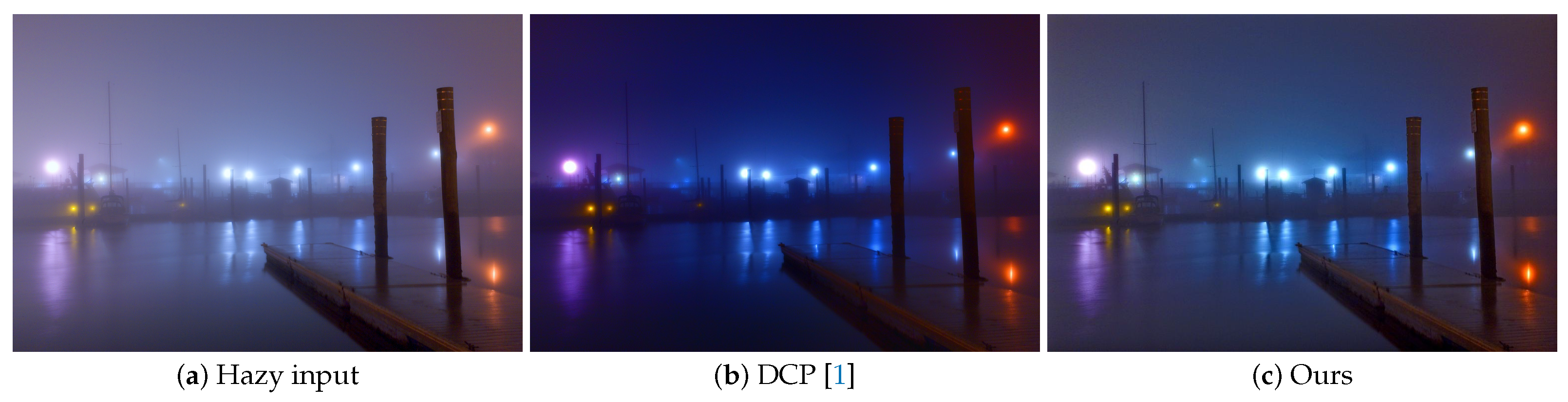
4.2. Visual Comparison

Almost all the defogging methods are able to produce a really good dehazed result by removing fog from a general outdoor image. Visual comparison is a common way to evaluate the performance of defogging methods. We compared some real-world images to ones obtained by some with the state-of-the-art dehazing methods.

First, we compared our proposed method with Meng et al.’s method [17] on the “Mountain” image suffering from a light fog. As shown in Figure 7, we can observe that our dehazed image is comparable with one produced by [17]. Then, we tested our method and eight state-of-the-art methods [1,4,9,10,13,18,19,20,21,22] on two real-world images of “ny12” and “ny17”, with smooth-depth scenes, as shown in Figure 8 and Figure 9. As shown, the results by Tan [18] have some over-enhanced regions. The methods of [4] cannot remove the haze completely, Nishino et al.’s method produces some color distortions, and the other results are relatively acceptable.

Second, we compare the proposed method with recent state-of-the-art methods [10,23,24,25,26,27,28,29,30]. From Figure 10, we can see that the results of RF [23] and CAP [10] tend to retain haze. The results of learning-based methods [28,29,30] also retain haze. The reason for learning based methods can not remove haze from real haze images is that they have a problem of domain shirt. The learning-based methods are trained on synthesized data, which are different form real hazy images. The proposed method improves the dehazed quality via multi-scale information.

We highlight the advantage of the proposed method in Figure 11. The BCCR [17] removes halos via contextual regularization. Our method removes halos via sparse coding, which is much faster than contextual regularization. As shown in Figure 11, we can see that the proposed method obtains a more natural result and avoids the halo artifact well. We also show a night hazy image dehazing in Figure 12. As we can see from Figure 12, the proposed method can keep more details than the DCP. The results of restoration by the proposed method are brighter than the results of using DCP [1].

4.3. Quantitative Comparison

In this section, we conduct some quantitative comparisons for the real-world images in Figure 8 and Figure 9 by the non-reference metrics of [31].

Three metrics are from [31], which are “e”, “∑”, and “$\overline{r}$”. “e” is defined as

$$e=\frac{n_r-n_o}{n_o},$$

(9)

where $n_o$ and $n_r$ denote respectively the cardinality of the set of visible edges in the original image and in the contrast-restored image. “∑” is defined as:

$$\sum =\frac{n_s}{di{m}_x\ast di{m}_y},$$

(10)

where $di{m}_x$ and $di{m}_y$ denote respectively the width and the height of the image, the number $n_s$ of pixels which are saturated (black or white) after applying the contrast restoration but were not before. “$\overline{r}$” is defined as

$$\overline{r}=exp[\frac{1}{n_r}\sum log{r}_i],$$

(11)

where $r_i$ is the rate of gradients between the input image and the output image. Specifically, the indicator “e” represents the newly visible edges ratio after restoration, the indicator “∑” represents the percentage of pixels which are completely white or dark after restoration, and “$\overline{r}$” expresses the quality of the recovered contrast. Higher values of “e” and “$\overline{r}$” are better, while a lower value of “∑” is better.

As shown in

Table 1. Quantitative comparisons on the real-world images of “ny12” and “ny17” using e, ∑ and $\overline{r}$ in [31].

Image	Tan			Fatta			Kopf et al.			He et al.			Tarrel et al.			Ancuti et al.			Choi et al.			Ours
	e	∑	$\overline{\mathit{r}}$	e	∑	$\overline{\mathit{r}}$	e	∑	$\overline{\mathit{r}}$	e	∑	$\overline{\mathit{r}}$	e	∑	$\overline{\mathit{r}}$	e	∑	$\overline{\mathit{r}}$	e	∑	$\overline{\mathit{r}}$	e	∑	$\overline{\mathit{r}}$
ny12	−0.14	0.02	2.34	−0.06	0.09	1.32	0.05	0.00	1.42	0.06	0.00	1.42	0.07	0.0	1.88	0.02	0.00	1.49	0.09	0.00	1.56	0.26	0.00	1.42
ny17	−0.06	0.01	2.22	−0.12	0.02	1.56	0.01	0.01	1.62	0.01	0.00	1.65	−0.01	0.0	1.87	0.12	0.00	1.54	0.03	0.00	1.49	0.15	0.00	1.59

, the compared methods cannot achieve better results according to the indicator ‘e’, only our method, DCP [1], Kopf et al.’s approach, Tarel et al.’s approach, Choi et al.’s approach and Ancuti et al.’s approach [13] produced positive values for this metric. The proposed method achieves the highest value of ‘e’, which indicates that the proposed method achieves better visibility enhancement. The result of Tan, Ancuti, and Tarel was due to oversaturation, while Kopf, DCP, and the proposed method achieve a reasonable enhancement. In addition, our results obtain small values of the non-reference metric of ‘∑’, which means that our algorithm generates less oversaturated regions.

5. Conclusions

In this paper, we proposed a novel method to remove haze from a single hazy image using sparse representation for contextual regularization, which can greatly reduce the halos and block artifacts in the dehazed results. Comparing with a series of the state-of-the-art dehazing methods, extensive experimental results on the hazy images illustrate that our method can generate high-quality dehazed results with vivid color, finer image structures, and local details.

References

1. He, K.; Sun, J.; Tang, X. Single image haze removal using dark channel prior. IEEE Trans. Pattern Anal. Mach. Intell. 2011, 33, 2341–2353. [Google Scholar] [PubMed]
2. Schechner, Y.Y.; Narasimhan, S.G.; Nayar, S.K. Instant dehazing of images using polarization. IEEE Comput. Soc. Conf. Comput. Vis. Pattern Recognit. CVPR 2001, 1, 325–332. [Google Scholar]
3. Kopf, J.; Neubert, B.; Chen, B.; Cohen, M.; Cohen-Or, D.; Deussen, O.; Uyttendaele, M.; Lischinski, D. Deep photo: Model-based photograph enhancement and viewing. ACM Trans. Graph. TOG 2008, 27, 32–39. [Google Scholar]
4. Fattal, R. Single image dehazing. ACM Trans. Graph. 2008, 27, 1–9. [Google Scholar] [CrossRef]
5. Kratz, L.; Nishino, K. Factorizing Scene Albedo and Depth from a Single Foggy Image. In Proceedings of the IEEE International Conference on Computer Vision (ICCV), Kyoto, Japan, 29 September–2 October 2009; pp. 1701–1708. [Google Scholar]
6. Shanmugapriya, S.; Valarmathi, A. Efficient fuzzy c-means based multilevel image segmentation for brain tumor detection in MR images. In Design Automation for Embedded Systems; Springer: Berlin/Heidelberg, Germany, 2018. [Google Scholar]
7. Versaci, M.; Calcagno, S.; Morabito, F. Fuzzy geometrical approach based on unit hyper-cubes for image contrast enhancement. In Proceedings of the 2015 IEEE International Conference on Signal and Image Processing Applications (ICSIPA), Kuala Lumpur, Malaysia, 19–21 October 2015. [Google Scholar]
8. Gibson, K.B.; Nguyen, T.Q. An analysis of single image defogging methods using a color ellipsoid framework. EURASIP J. Image Video Process. 2013, 2013, 1–14. [Google Scholar] [CrossRef] [Green Version]
9. Fattal, R. Dehazing using color-lines. ACM Trans. Graph. TOG 2014, 34, 1–14. [Google Scholar] [CrossRef]
10. Zhu, Q.; Mai, J.; Shao, L. A Fast Single Image Haze Removal Algorithm Using Color Attenuation Prior. IEEE Trans. Image Process. 2015, 24, 3522–3533. [Google Scholar] [PubMed] [Green Version]
11. Li, Z.; Zheng, J. Edge-Preserving Decomposition-Based Single Image Haze Removal. IEEE Trans. Image Process. 2015, 24, 5432–5441. [Google Scholar] [CrossRef] [PubMed]
12. Ancuti, C.O.; Ancuti, C.; Hermans, C.; Bekaert, P. A fast semi-inverse approach to detect and remove the haze from a single image. In Computer Vision–ACCV 2010; Lecture Notes in Computer Science; Springer: Berlin/Heidelberg, Germany, 2010; pp. 501–514. [Google Scholar]
13. Ancuti, C.O.; Ancuti, C. Single image dehazing by multi-scale fusion. IEEE Trans. Image Process. 2013, 22, 3271–3282. [Google Scholar] [CrossRef] [PubMed]
14. Elad, M.; Aharon, M. Image denoising via sparse and redundant representations over learned dictionaries. IEEE Trans. Image Process. 2006, 15, 3736–3745. [Google Scholar] [CrossRef] [PubMed]
15. Yang, J.; Wright, J.; Huang, T.S.; Ma, Y. Image super-resolution via sparse representation. IEEE Trans. Image Process. 2010, 19, 2861–2873. [Google Scholar] [CrossRef] [PubMed]
16. Koschmieder, H. Theorie der horizontalen Sichtweite, Beiträge zur Physik der freien Atmosphäre. Meteorol. Z 1924, 12, 33–53. [Google Scholar]
17. Meng, G.; Wang, Y.; Duan, J.; Xiang, S.; Pan, C. Efficient image dehazing with boundary constraint and contextual regularization. In Proceedings of the IEEE International Conference on Computer Vision (ICCV), Sydney, Australia, 1–8 December 2013; pp. 617–624. [Google Scholar]
18. Tan, R.T. Visibility in bad weather from a single image. In Proceedings of the IEEE Conference on Computer Vision and Pattern Recognition (CVPR), Anchorage, AK, USA, 24–26 June 2008; pp. 1–8. [Google Scholar]
19. Tarel, J.P.; Hautiere, N. Fast visibility restoration from a single color or gray level image. In Proceedings of the IEEE International Conference on Computer Vision (ICCV), Kyoto, Japan, 29 September–2 October 2009; pp. 2201–2208. [Google Scholar]
20. Nishino, K.; Kratz, L.; Lombardi, S. Bayesian defogging. Int. J. Comput. Vis. 2012, 98, 263–278. [Google Scholar] [CrossRef]
21. Wang, Y.K.; Fan, C.T. Single Image Defogging by Multiscale Depth Fusion. IEEE Trans. Image Process. 2014, 23, 4826–4837. [Google Scholar] [CrossRef] [PubMed]
22. Choi, L.K.; You, J.; Bovik, A.C. Referenceless Prediction of Perceptual Fog Density and Perceptual Image Defogging. IEEE Trans. Image Process. 2015, 24, 3888–3901. [Google Scholar] [CrossRef] [PubMed]
23. Tang, K.; Yang, J.; Wang, J. Investigating haze-relevant features in a learning framework for image dehazing. In Proceedings of the CVPR, Columbus, OH, USA, 24–27 June 2014; pp. 2995–3000. [Google Scholar]
24. Sulami, M.; Glatzer, I.; Fattal, R.; Werman, M. Automatic recovery of the atmospheric light in hazy images. In Proceedings of the ICCP, Cluj-Napoca, Romania, 4–6 September 2014. [Google Scholar]
25. Cai, B.; Xu, X.; Jia, K.; Qing, C.; Tao, D. Dehazenet: An end-to-end system for single image haze removal. TIP 2016, 25, 5187–5198. [Google Scholar] [CrossRef] [PubMed] [Green Version]
26. Ren, W.; Liu, S.; Zhang, H.; Pan, J.; Cao, X.; Yang, M.H. Single image dehazing via multi-scale convolutional neural networks. In Proceedings of the ECCV, Amsterdam, The Netherlands, 8–16 October 2016. [Google Scholar]
27. Berman, D.; Treibitz, T.; Avidan, S. Non-local image dehazing. In Proceedings of the CVPR, Las Vegas, NV, USA, 27–30 June 2016. [Google Scholar]
28. Li, B.; Peng, X.; Wang, Z.; Xu, J.; Feng, D. An All-in-One Network for Dehazing and Beyond. In Proceedings of the ICCV, Venice, Italy, 22–29 October 2017. [Google Scholar]
29. Zhang, H.; Patel, V.M. Densely Connected Pyramid Dehazing Network. In Proceedings of the CVPR, Salt Lake City, UT, USA, 18–23 June 2018. [Google Scholar]
30. Ren, W.; Ma, L.; Zhang, J.; Pan, J.; Cao, X.; Liu, W.; Yang, M.H. Gated Fusion Network for Single Image Dehazing. In Proceedings of the CVPR, Salt Lake City, UT, USA, 18–23 June 2018. [Google Scholar]
31. Hautière, N.; Tarel, J.P.; Aubert, D.; Dumont, E. Blind contrast enhancement assessment by gradient ratioing at visible edges. Image Anal. Stereol. J. 2008, 27, 87–95. [Google Scholar] [CrossRef]
Figure 1. An illustration of our proposed single image dehazing method on a real-world image. From left to right: the hazy input, the estimated transmission map by the proposed algorithm, and the dehazed image.
Atmosphere 12 01266 g001
Figure 2. An example of our proposed sparse contextual representation-based dehazing method. From left to right—the hazy input, the estimated transmission map by the proposed algorithm, and the dehazed image.
Atmosphere 12 01266 g002
Figure 3. An illustration of smoothing a piece-wise transmission map (a) with 15 atoms (b), 5 atoms (c) and 1 atom (d), respectively.
Atmosphere 12 01266 g003
Figure 4. The framework for our proposed method recovering the transmission map using sparse representation.
Atmosphere 12 01266 g004
Figure 5. Visual results on a real-world hazy image. For left to right, the hazy input, the estimated transmission map, and the dehazed result.
Atmosphere 12 01266 g005
Figure 6. The dehazing results on three typical images: (Top) the input haze images; (Middle) the recovered transmission maps; (Bottom) the dehazed images.
Atmosphere 12 01266 g006
Figure 7. Visual comparison with the Meng et al.’s method on the “Mountain” image: (Left) the input haze image; (Middle) Meng et al.’s result; (Right) our result.
Atmosphere 12 01266 g007
Figure 8. Visual comparisons on a real-world hazy image of “ny12”.
Atmosphere 12 01266 g008
Figure 9. Visual comparisons on a real-world hazy image of “ny17”.
Atmosphere 12 01266 g009
Figure 10. The dehazing result of the proposed method and state-of-the art methods on the real hazy images. The proposed method generates much clearer images with clearer structures and characters.
Atmosphere 12 01266 g010
Figure 11. The dehazing result of the proposed method and state-of-the art methods on the real hazy images. The proposed method generates much clearer images with clearer structures and characters.
Atmosphere 12 01266 g011
Figure 12. The dehazing result of the proposed method and state-of-the art methods on the real night hazy images. The proposed method generates much clearer images with clearer structures and characters.
Atmosphere 12 01266 g012