Single Image Atmospheric Veil Removal Using New Priors for Better Genericity

Abstract

From an analysis of the priors used in state-of-the-art algorithms for single image defogging, a new prior is proposed to obtain a better atmospheric veil removal. Our hypothesis is based on a physical model, considering that the fog appears denser near the horizon rather than close to the camera. It leads to more restoration when the fog depth is more important, for a more natural rendering. For this purpose, the Naka–Rushton function is used to modulate the atmospheric veil according to empirical observations on synthetic foggy images. The parameters of this function are set from features of the input image. This method also prevents over-restoration and thus preserves the sky from artifacts and noises. The algorithm generalizes to different kinds of fog, airborne particles, and illumination conditions. The proposed method is extended to the nighttime and underwater images by computing the atmospheric veil on each color channel. Qualitative and quantitative evaluations show the benefit of the proposed algorithm. The quantitative evaluation shows the efficiency of the algorithm on four databases with different types of fog, which demonstrates the broad generalization allowed by the proposed algorithm, in contrast with most of the currently available deep learning techniques.

1. Introduction

Visibility restoration of outdoor images is a well-known problem in both computer vision applications and digital photography, particularly in adverse weather conditions such as fog, haze, rain, and snow. Such weather conditions cause visual artifacts in the images such as loss of contrast and color shift, which contributes to reducing scene visibility. The lack of visibility can be detrimental for the performance of automated systems based on image segmentation [1] and object detection [2], and thus requires visibility restoration as a pre-processing [3]. With fog or haze, contrast reduction is caused by the atmospheric veil. With rain or snow, it is caused by the occlusion of the distant background by raindrops or snowflakes.

This paper proposes a single image dehazing method based on the Naka–Rushton function to treat the fog presents near the horizon in real images and to generalize to different kinds of fog represented in the databases of the evaluation section. In addition, a simple solution is added to process nighttime and underwater images, allowing further generalization to different kinds of particles and illumination conditions. Some of these contributions have been proposed in [4]. This paper proposes three contributions:

• The use of a Naka–Rushton function in the inference of the atmospheric veil to restore the fog near the horizon without restoring the part near the camera. The parameters of this function are estimated from the characteristics of the input foggy image.
• The proposed algorithms also address spatially uniform veils, and generalize to different kinds of fog, by the help of an interpolation function.
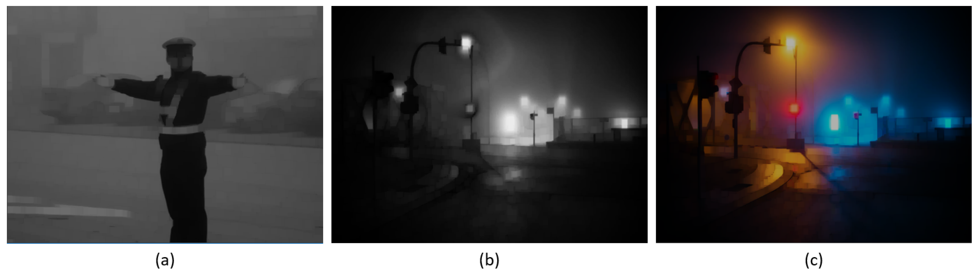
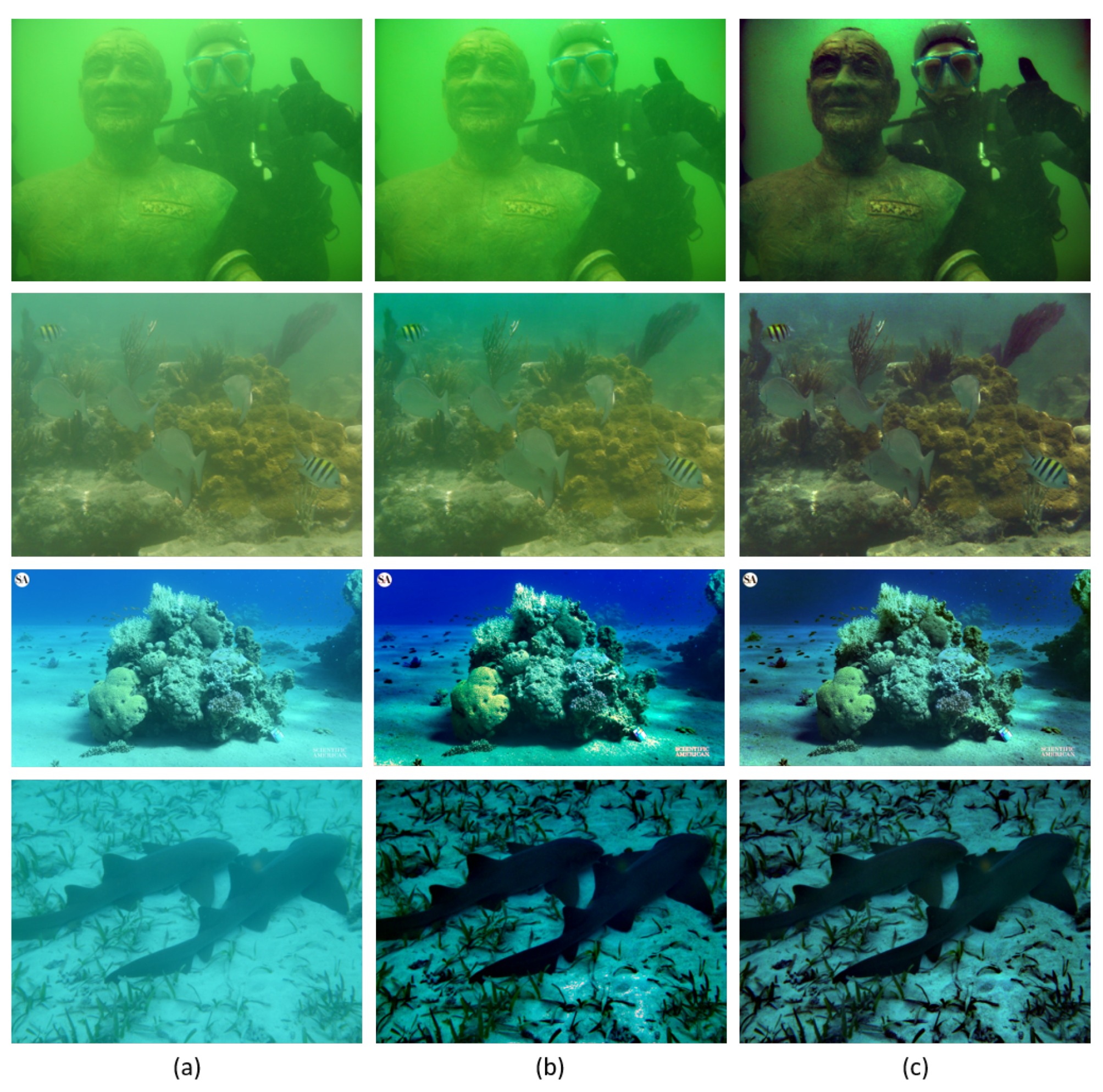
• Applying our method on each color channel addresses the local variations of the color of the fog. This allows for restoring images with color distortions due to dust and pollution, as well as nighttime and underwater images.

The paper is organized as follows: Section 2 introduces the problem and related works. Section 3 presents the proposed visibility restoration method and Section 4 shows experimental results with qualitative and quantitative evaluations and comparisons.

2. Related Works

2.1. Fog Visual Effect

Koschmieder’s law is a straightforward optical model that describes the visual effects of the scattering of daylight by the particles fog is made of. When fog and illumination are homogeneous along a light path going through x, the model is:

$$I\left(x\right)=J\left(x\right)t\left(x\right)+A(1-t(x\left)\right)$$

(1)

where $I\left(x\right)$ is the foggy image, $J\left(x\right)$ the fog-free image, A the sky intensity, and $x=(u,v)$ denotes the pixel coordinates. The transmittance $t\left(x\right)$ describes the percentage of light that is not scattered:

$$t\left(x\right)=e^{-kd\left(x\right)}$$

(2)

where k is the extinction coefficient that is related to the density of fog, and $d\left(x\right)$ is the distance between the camera and the objects in the scene. Equations (1) and (2) are valid only together. The atmospheric veil is the second term in (1).

2.2. Daytime Image Defogging

Single image defogging algorithms can be divided into two categories. Image enhancement algorithms use ad-hoc techniques to improve the image contrast such as histogram equalization and retinex, but they do not account for scene depth. Visibility restoration, on which we focus, are model-based and use Koschmieder’s law. Since depth is unknown, the problem is an ill-posed inverse problem that requires priors to be solved. Priors may be introduced as constraints or using a learning dataset.

He et al. [5,6] introduced the Dark Channel Prior (DCP) for a method dedicated to color images. The idea is that fog-free outdoor images contain pixels with very low intensity in at least one of the three color channels at any location. It was also proposed to refine the transmission map by a filtering guided by the input image to avoid halos in the final result [7,8]. Many works were inspired by the DCP method and brought some improvements [9,10,11,12,13,14]. Li et al. [11] proposed an edge preservation technique to improve the transmission map estimation. They split the dark channel of the foggy image into two layers with a guided filter. This method reduces artifacts and noises in the restored images. Zhu et al. [12] developed a method to estimate the transmission map by minimizing the energy function, in order to fully exploit the DCP. This method combines the DCP with piecewise smoothness. Recently, Jackson et al. [13] proposed a fast dehazing method based on Rayleigh’s scattering theory, in order to estimate the transmission map with a fast-guided filter. This method reduces the computational time and provides good results. Zhang et al. [14] proposed a criterion-based segmenting the transmission map into foreground-background regions, in order to reduce halo artifacts and computational complexity.

Tarel et al. [15] proposed two priors: the fog is white, and locally smooth. As pointed out in [16], the first prior leads to the use of the channel with the minimum intensity among the color channels, as in [6]. The second prior leads to the use of a local filter, preferably one that preserves both edges and corners. This fast algorithm allows restoration of color and gray-scale images. In [16], a flat terrain assumption was introduced in order to avoid over-restoration in the bottom part of the image. It works well on objects close to the camera but requires the height of the horizon line to be approximately known. To tackle the same difficulty, a modulation function of the atmospheric veil was introduced to deal with road traffic scenes [17]. This modulation function is a function of the pixel position, and thus its parameters must be tuned according to the observed scene.

Ancuti et al. [18,19] proposed a fusion-based approach to estimate the atmospheric veil. It combines several feature images and weight maps derived from the original input image. The prior lies implicit in the way the fusion is achieved. Wang et al. [20] proposed a method based on a so-called color attenuation prior, where the atmospheric veil is estimated using a linear combination of features extracted locally in the input foggy image.

Zheng et al. [21] proposed an adaptative structure decomposition method integrated multi-exposure image fusion for single image dehazing. A set of underexposed images are extracted from different gamma correction images to fused into haze-free images. This method avoids using a physical model and priors estimation. An extension of this research is proposed by Zhu et al. [22] with the aim of reducing over-exposed areas located in hazy regions, by balancing image luminance and saturation, and preserving details and the overall structure of the restored image.

In the last five years, learning-based methods have been proposed for defogging usually based on Convolutional Neural Networks (CNN) with supervised training [23,24,25,26,27]. Cai et al. [23] proposed a trainable model to estimate the transmission map and recover clear images using the Koschmieder’s model. However, the intermediate steps for estimating the parameters can generate reconstruction errors and provide inaccurate transmission maps. To overcome this issue, Li et al. [26] proposed a fully end-to-end model to directly generate clear images from foggy images with a joint estimation of the transmission map and the atmospheric veil. Fog is a rather unpredictable phenomenon, so building a large and representative training dataset with pairs of images with and without fog is very difficult. This leads to generalization problems. More recently, GAN networks have been used [28,29], with partially supervised training databases, but the learning control is complicated. Fog removal being a pre-processing, fast and computationally inexpensive algorithms are usually required. We thus focus here on algorithms with very few parameters to be learned.

2.3. Hidden Priors in the DCP Method

In DCP [5,6], a widely used parameter called $\omega$ was clearly introduced in the transmission map computation:

$$t\left(x\right)=1-\omega \underset{c}{min}\left(\underset{y\in \Omega \left(x\right)}{min}\left(\frac{I^c\left(y\right)}{A^c}\right)\right)$$

(3)

where $\Omega \left(x\right)$ is the local patch centered on x, c the color channel, A the sky intensity, and I the image intensity. This parameter was introduced to mitigate over-restoration, and it is usually set to $\omega =0.95$. According to [5], it maintains a small amount of haze in the distance, producing more natural results.

This parameter is actually a prior and needs to be explicit. First, let us propose a different interpretation of $\omega$. The term ${min}_c\left({min}_{y\in \Omega \left(x\right)}\left(I^c\left(y\right)\right)\right)$ in the transmittance Equation (3) is a first estimation of the atmospheric veil, based on the white fog and the locally smooth fog priors. The result is a mixture between the actual atmospheric veil and the luminance of objects in the scene. Let us name it the “pre-veil”. The percentage of the pre-veil which corresponds to the real atmospheric veil is unknown; it is assumed to be constant and equal to $\omega$ across the image. Therefore, $\omega$ can be explicitly described as a prior parameter: it is the assumed constant percentage of the atmospheric veil in the pre-veil map. We test the validity of this prior in the next section.

3. Single Image Atmospheric Veil Removal

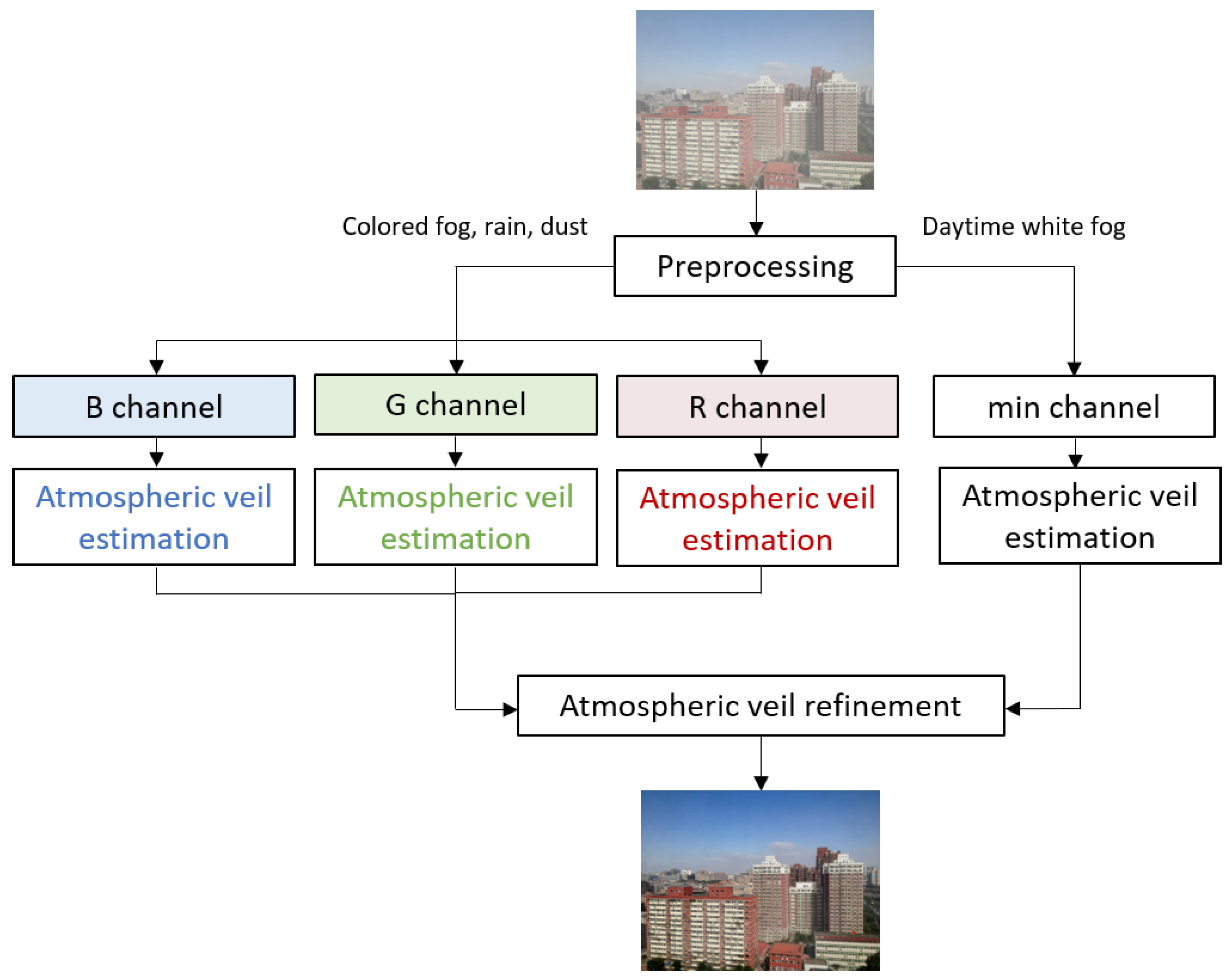
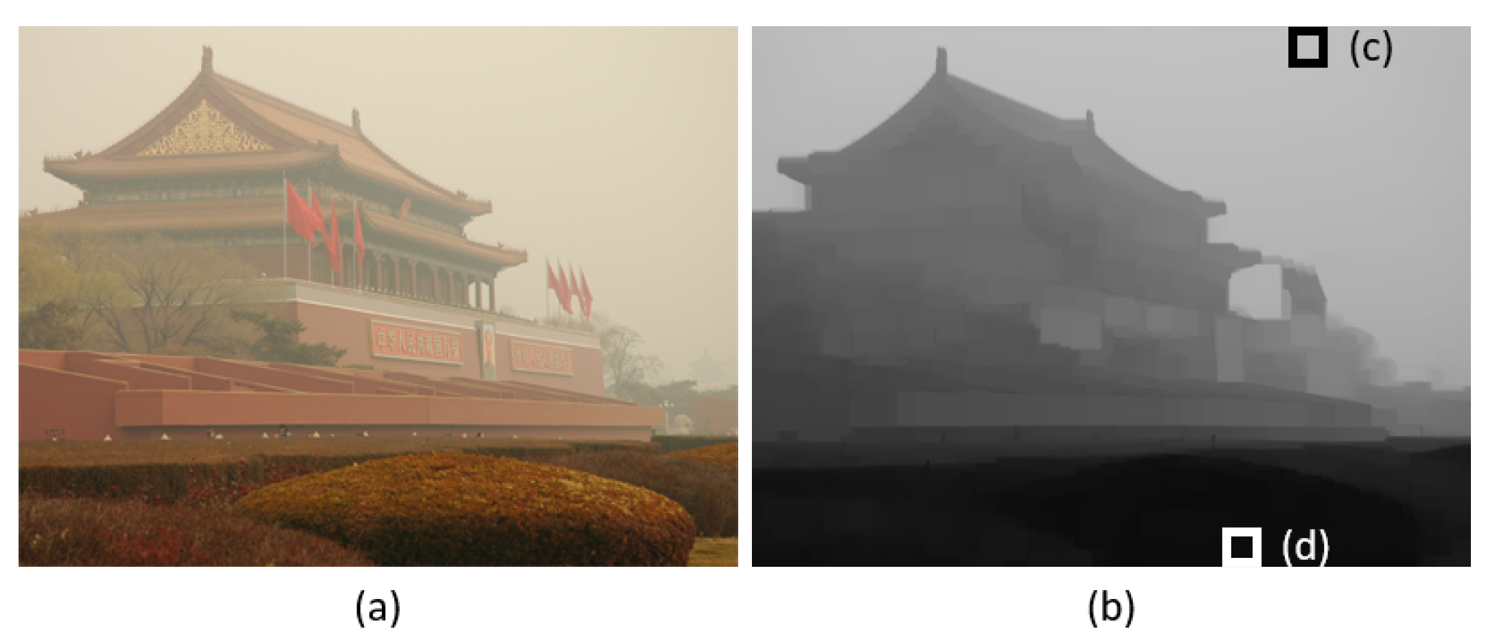
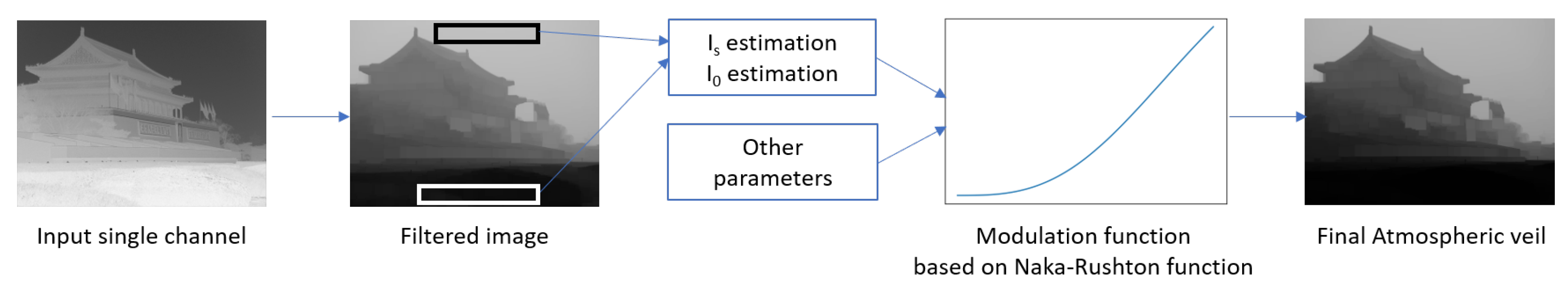
3.1. Algorithm Flowchart

The proposed algorithm first needs a prior about the nature of the observed scene. Two categories are considered:

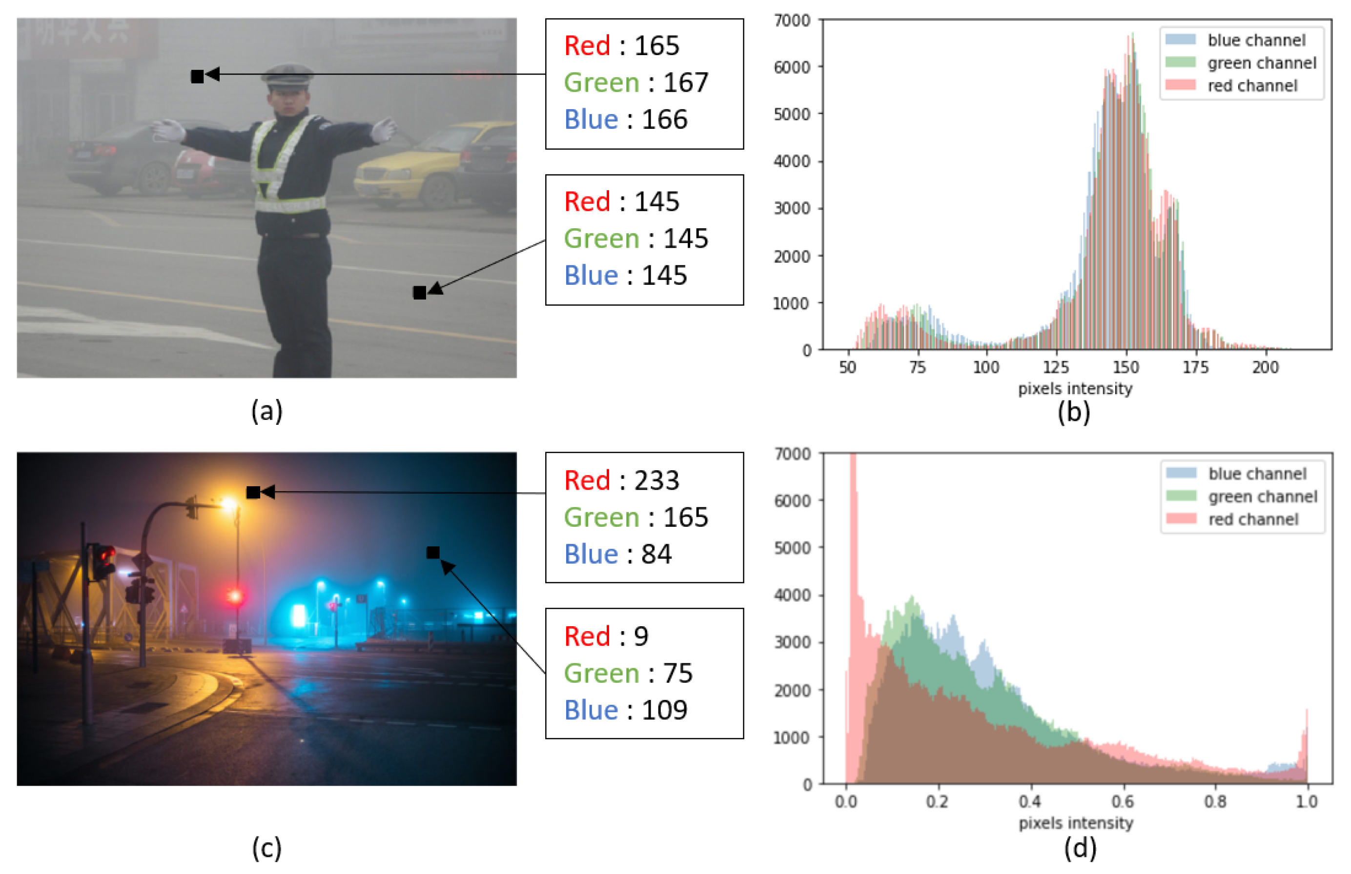
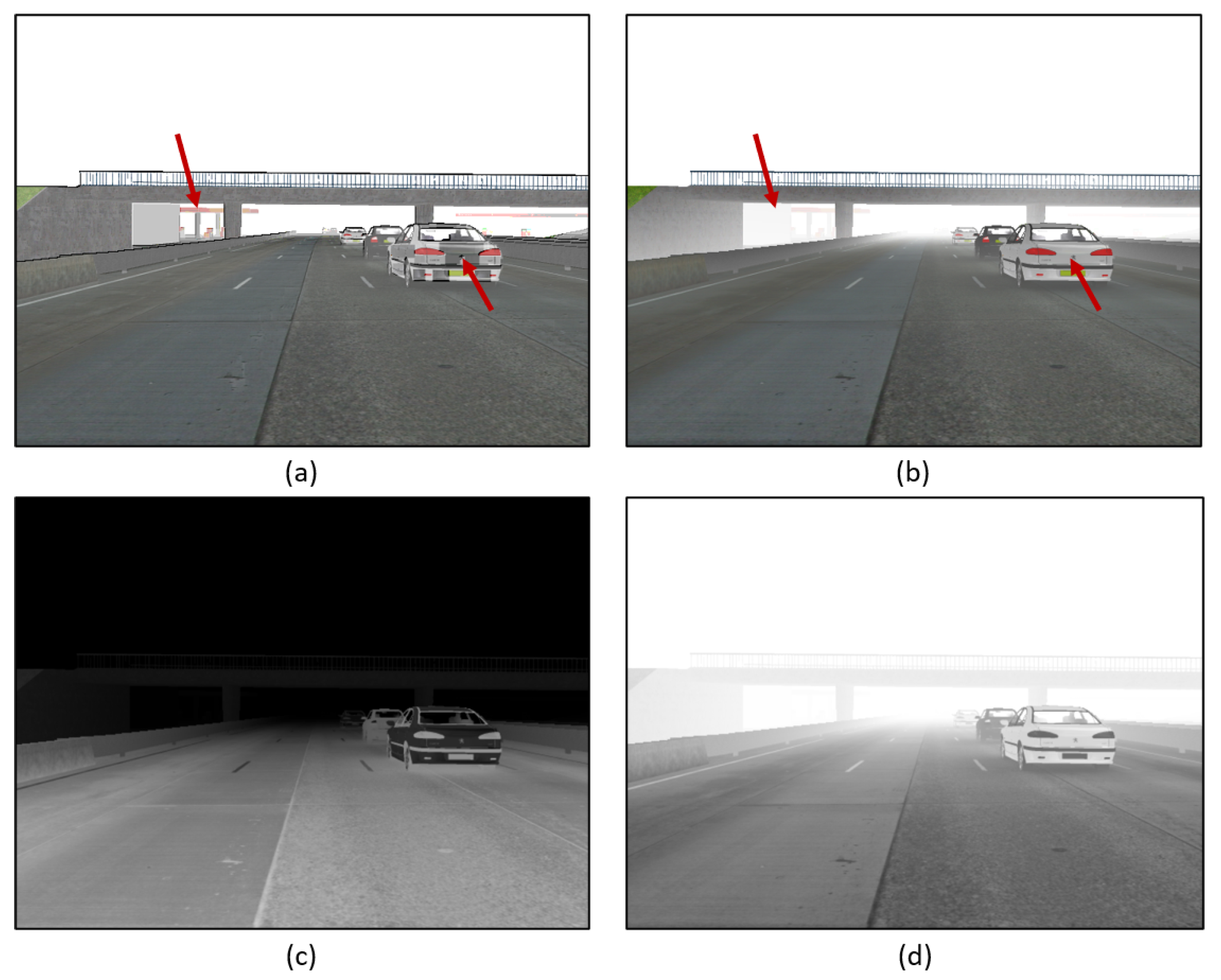
• Daytime white fog: the pre-veil is computed from the color channel that has the minimum intensity. The fog is assumed to be homogeneous or may vary slowly in density from one pixel to another, but not in the viewing frustum of a pixel.
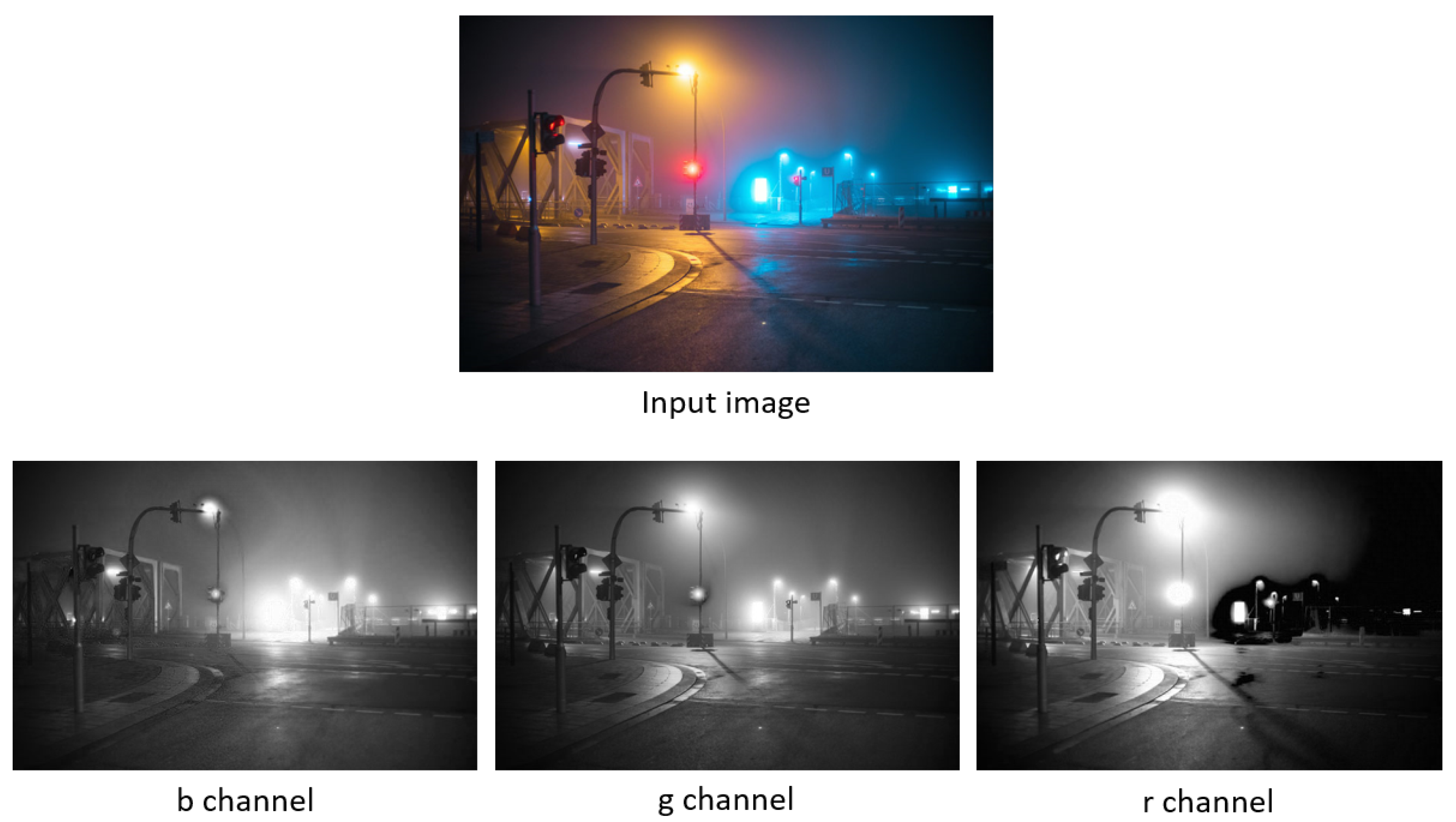
• Colored fog, rain, smoke, dust: the airlight cannot be assumed to be pure white, so color channels are processed separately by simply splitting the images into RGB channels. Then, the atmospheric veil is computed on each color channel. The density of airborne particles may vary slowly from a pixel to another.

The flowchart of the proposed algorithm is shown in Figure 1. From a pre-veil step, the atmospheric veil is obtained with the Naka–Rushton function, with parameters computed from the input image features. The atmospheric veil is then refined by applying a filtering guided by the input image. The final step consists of the computation of the restored image by inversing Koschmieder’s law on the input image with the previously obtained atmospheric veil map.

3.2. Is the Use of ω a Valid Prior?

The usual way to compute the atmospheric veil from the pre-veil is to apply the parameter $\omega$. To test the validity of this prior, we have to look at the link between the intensities in the true veil and in the pre-veil images. This can only be achieved with a synthetic image database, and, to achieve this, we used the generator of the FRIDA dataset [16]. In these synthetic images, the veil is computed using Koschmieder’s law from the scene depth map. Thus, the atmospheric veil map can be computed for each generated foggy image. An advantage is that it is possible to generate images with homogeneous or heterogeneous fog, and homogeneous or heterogeneous illumination. Figure 2 shows the histograms of fifty such foggy images, with the pre-veil image intensities on the horizontal axis, and the intensities of the ground truth atmospheric veil on the vertical axis. Figure 2 and Figure 3a show that the link between foggy pixel intensities and associated veil intensities is roughly affine. The intensity of the atmospheric veil is high in the sky region, and it is low in the ground region that is closer to the camera. Since this variation is affine, it cannot be modeled well with a constant parameter such as $\omega$. A function would be more relevant.

3.3. Modulation Function as a Prior

To avoid over-restoration at the bottom of the image, but, to ensure that the restoration is maximum at the top of the image, a modulation function f is necessary to compute the atmospheric veil from the pre-veil. This function should be smooth to avoid visual artifacts in the restored image.

From Figure 3a, the following constraints are proposed to choose an appropriate function f which will appropriately modulate the pre-veil:

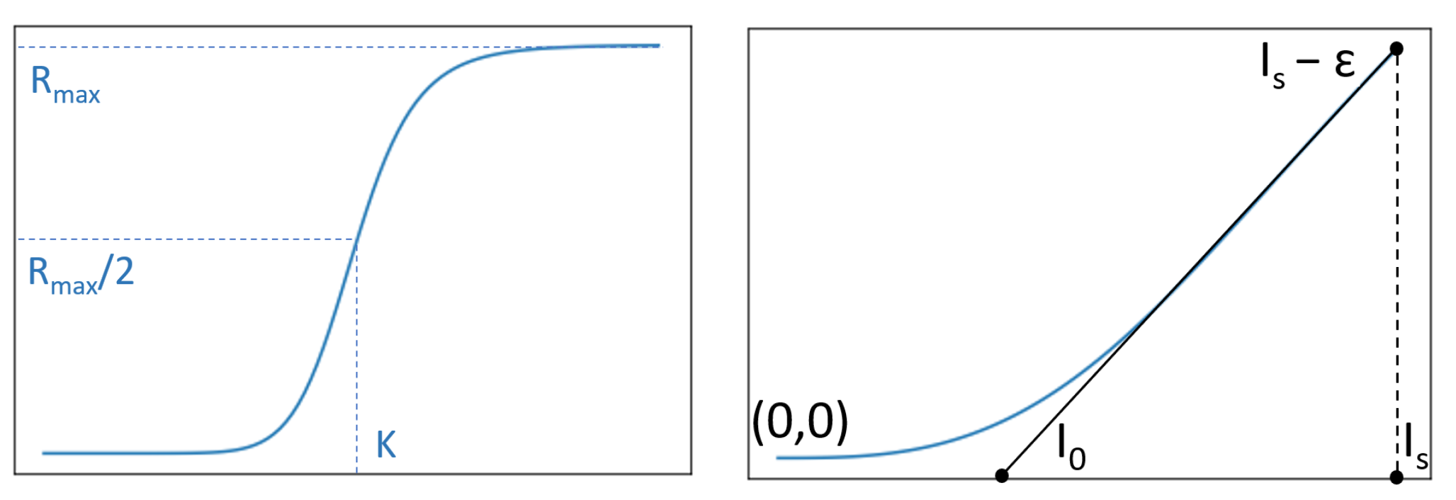
• The function f should be roughly linear on a large range of intensities. This range is denoted $[I_0,I_s]$. We introduce here the slope a of f at $I_s$, i.e., $f^{\prime }\left(I_s\right)=a$.
• The function is close to zero on the intensity range $[0,I_0]$, i.e., for the intensities of pixels looking at objects that are close to the camera.
• The function and the restored image must not be negative.
• $I_s$ is the intensity of the clearest (sky) region. To avoid too dark values in the corresponding areas, $f\left(I_s\right)$ should be a little lower than $I_s$.
  We thus introduce a parameter $ϵ$ such that $f\left(I_s\right)=I_s-ϵ$ in order to preserve the sky. $ϵ$ is smoothly estimated as a function of $I_s$.
  $ϵ$ = 0.3 when $I_s$ is high ($I_s$ > 0.8), $ϵ$ = 0.05 when $I_s$ is low ($I_s$ < 0.6). Between these values, $ϵ=\frac{0.3I_s}{ma{x}_{I_s}}$

Among the different functions we tested, the Naka–Rushton [30] function was the easiest to tune. This function was first introduced to describe the biological response of a neuron, and was further used in computer graphics for the tone-mapping problem. It is defined as:

$$R\left(x\right)=R_{max}\frac{x^n}{x^n+K^n}$$

(4)

where $R_{max}$ is the upper-bound of the Naka–Rushton function, K is the horizontal position of the inflection point, and n is related to the slope at the inflection point (see Figure 4). The shape of the first part of the curve in Figure 4 (left) fits our needs, as shown in Figure 4 (right). The inflexion point with coordinates $(K,\frac{R_{max}}{2})$ should correspond to the modulation function f at $I_s$. Indeed, $I_s$ is the maximum of the pixel intensities in the input image. Then, the constraint f($I_s$) = $I_s-ϵ$ is used to avoid artifacts in the sky region. From this, the value of K was set to $I_s$.

3.4. Naka–Rushton Function Parameters

$R_{max}$, K, and n are the parameters of the Naka–Rushton function, whereas the parameters of the modulation function f are $I_0$, $I_s$, and $ϵ$. In the previous section, K was set to $I_s$. Following constraint 4 in Section 3.3, $f\left(I_s\right)$ is set to $I_s-ϵ$. Thus, $R_{max}=2(I_s-ϵ)$. The slope at $I_s$ is set to a. This slope in the Naka–Rushton function being $\frac{n{R}_{max}}{4K}$ (obtained by deriving the Naka–Rushton function), we have $n=\frac{2I_{s}a}{I_s-ϵ}$. It follows that $a=\frac{I_s-ϵ}{I_s-I_0}$. The parameter a was calculated as the slope between the points of coordinates ($I_0$, 0) and ($I_s$, $I_s-ϵ$) (see the right image in Figure 4).

Finally, the proposed modulation function f is:

$$f\left(x\right)=f_0\frac{x^n}{x^n+K^n}$$

(5)

where $f_0=2(I_s-ϵ)$, $K=I_s$, $n=\frac{2I_{s}a}{I_s-ϵ}$ and $a=\frac{I_s-ϵ}{I_s-I_0}$. This modulation function has only three parameters: $I_0$, $I_s$, and $ϵ$. The last one must be set to a small value, and the other two can be computed from the input image.

$I_s$ is the intensity of the sky and $I_0$ is the intensity of the ground close to the camera. We have investigated how $I_0$ and $I_s$ can be best estimated (see Figure 5). Take the maximum of the image intensities for $I_s$, and the minimum for $I_0$ is too sensitive to noise. Therefore, $I_0$ and $I_s$ are computed by taking, respectively, the minimum and the maximum of the input foggy image after applying a morphological closing followed by a morphological opening. Figure 6 schematizes the process of estimating atmospheric veil.

3.5. Interpolation between Two Models

Several analyses carried out on different kinds of databases have shown that the proposed algorithm is less efficient when the veil is spatially close to uniform. Although these types of images are not very realistic, our main algorithm has been modified in order to deal with veils spatially close to uniform with the aim of generalizing the proposed method. To take this class of images into account, we propose a new version of our algorithm, which is improved for images with a spatially uniform veil, and roughly unchanged for a depth-dependent fog.

When the veil is spatially close to uniform, as with satellite images, the most suitable function to use for restoration is a constant, as the fog has a nearly constant depth. To address this situation, we define $g\left(x\right)=I_0$, which estimates this constant function.

$I_0$ is set to the minimum value in the pre-veil (see Figure 5), so that it gives the intensity of the darker areas in the filtered image. In “normal” fog, this value is expected to be low, representative of close-by objects without much fog. The veil is considered to be spatially constant on the image when $I_0$ is greater than a fixed threshold (0.2 in the following).

We have considered several methods to take uniform veils into account: their common feature is that they interpolate between two functions, f and g. Two functions have been tested for f: the Naka–Rushton function from Equation (5), named $f_1$ in the following, and a function matching the affine part of our Naka–Rushton-like function: $f_2\left(x\right)=\frac{x-I_0}{1-I_0}$, which is simpler and close to the shape of the histogram (Figure 3).

The interpolation takes the form:

$$k_{m,p,i}\left(x\right)=\frac{I_0^{p}g\left(x\right)+{(m-I_0)}^p{f}_i\left(x\right)}{I_0^p+{(m-I_0)}^p}$$

(6)

The free parameters (m and p) allow for tuning the weighting of the two functions. High values of p lead to a sharp switch between $f_i$ and g; preliminary tests showed that the best values for these parameters were $p=2$ and $m=0.3$.

We compared five interpolation methods in terms of the SSIM and PSNR indexes on the same datasets (

Table 1. Comparison of the SSIM and PSNR indexes on the four datasets with the five interpolation functions listed in the text before the table. I is for Interpolation, S for Switch. The two best results are in bold.

SSIM|PSNR
Functions	FRIDA	SOTS	NTIRE20	O-HAZE
$f_1$	0.81|13.34	0.85|18.40	0.50|13.22	0.64|16.32
$I(f_1,g)$	0.78|11.65	0.93|24.40	0.49|12.75	0.66|16.57
$I(f_2,g)$	0.78|11.74	0.93|24.00	0.48|12.57	0.66|16.47
$S(f_1,g)$	0.79|13.09	0.91|23.01	0.49|12.85	0.66|16.62
$S(f_2,g)$	0.79|13.29	0.88|21.62	0.46|12.01	0.64|16.07

):

• Our modulation function: $f_1\left(x\right)$;
• An interpolated function between $g\left(x\right)$ and $f_1\left(x\right)$;
• An interpolated function between $g\left(x\right)$ and $f_2\left(x\right)$;
• A switch between $g\left(x\right)$ and $f_1\left(x\right)$ at the threshold $x=I_0$;
• A switch between $g\left(x\right)$ and $f_2\left(x\right)$ at the threshold $x=I_0$.

Table 1 shows that $f_1$ alone performs well on both the FRIDA and the NTIRE20 datasets, but the interpolated functions $I(f_1,g)$ and $I(f_2,g)$ provide better results on the SOTS and O-HAZE datasets. Using $f_2$ instead of $f_1$ does not improve the algorithm’s performance, nor does using a sharp switch between $f_{1|2}$ and g. The results on the datasets where the veil is spatially close to uniform (SOTS and O-HAZE) show that the constant function is a good alternative for this type of fog. The modulation function interpolated between a constant and our Naka–Rushton-like function $I(f_1,g)$ deals with several types of fog, and it is competitive with the other algorithms listed in the Section 4.1 on all datasets. In the evaluation part, this interpolated function is called I.

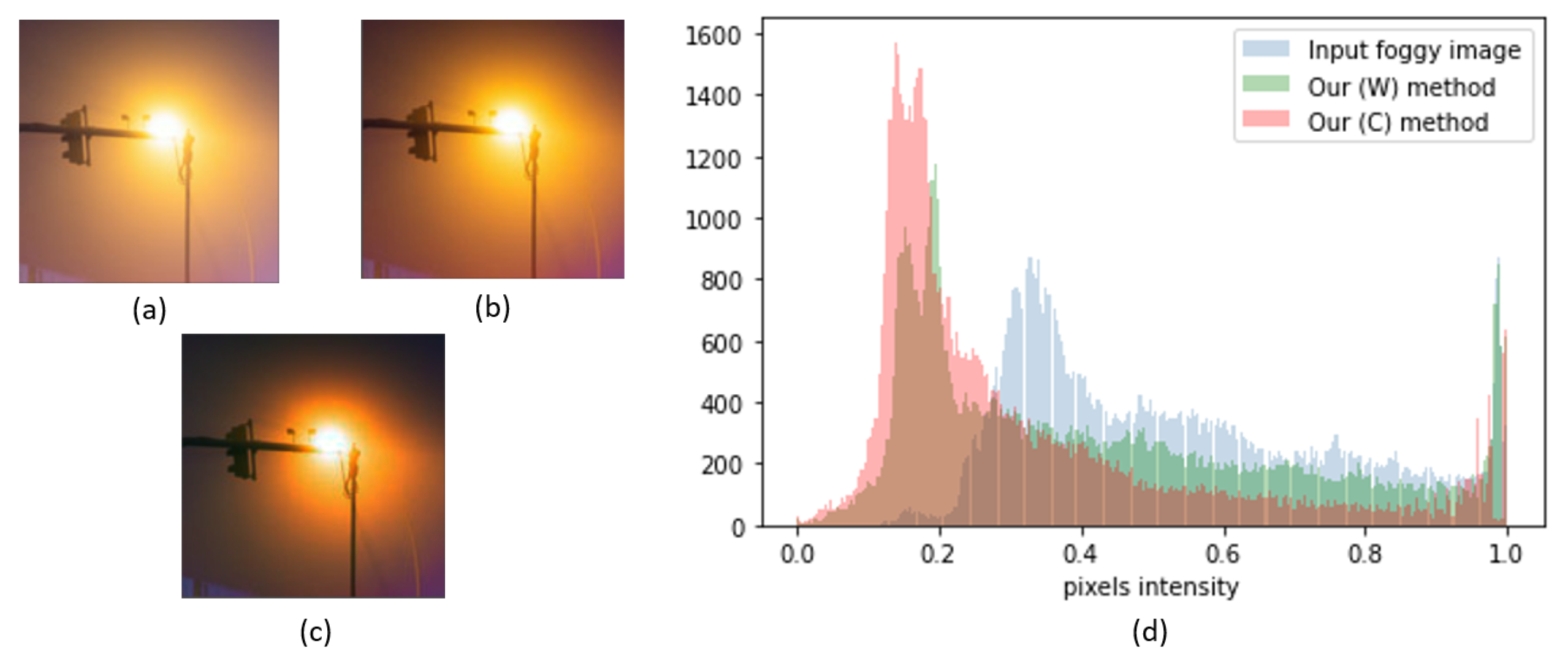
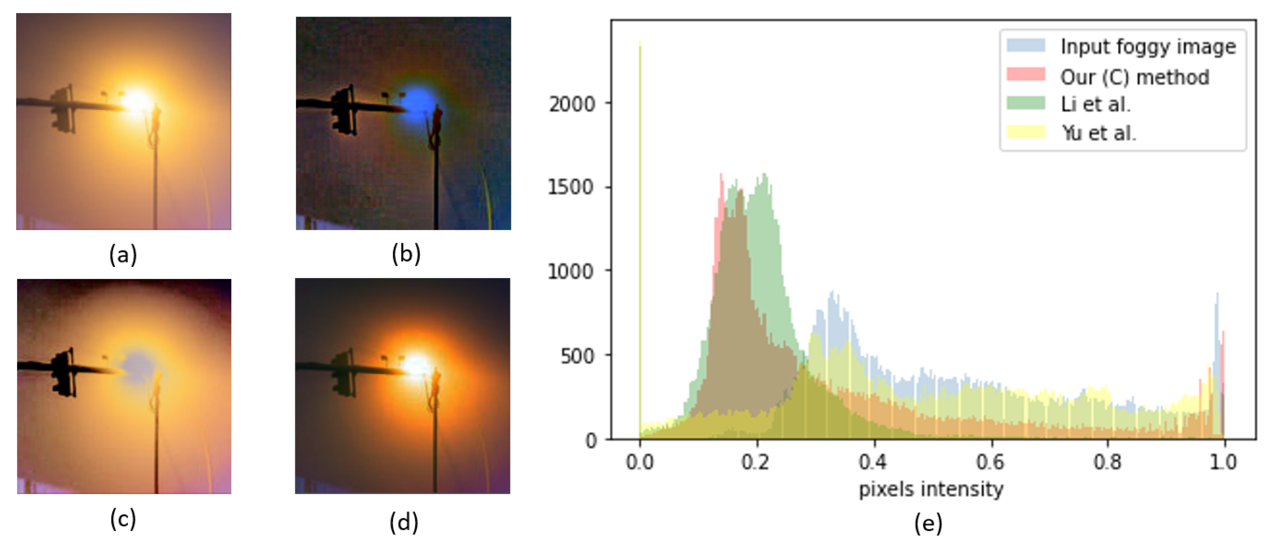
3.6. Beyond the White Fog Prior

Koschmieder’s law applies along light paths when the fog and the illumination are homogeneous. In situations that do not meet these conditions, Koschmieder’s law is no longer valid. In the nighttime images, for instance, scattering causes luminous halos around light sources which makes for a non-uniform atmospheric veil, even in homogeneous fog. Underwater images also suffer from large illumination variations due to light absorption with depth. Several works override these theoretical limits and apply Koschmieder’s law on nighttime and underwater images.

Many algorithms have been proposed for nighttime haze removal. Li et al. [31] proposed an algorithm to remove the glow by splitting it from the rest of the image. In [32], defogging being a local process, a multi-scale fusion approach was proposed to restore foggy nighttime images. Zhang et al. [33] proposed a maximum direct reflectance (MRP) method to estimate ambient illuminance based on the following assumption: for most daytime haze-free image patches, each color channel has a very high intensity at certain pixels. Very recently, Lou et al. [34] proposed a novel color correction technique based on MRP and used an inverse correlation between the transmittance and haze density to estimate the transmission map.

Even though interesting results can be obtained outside the validity domain of Koschmieder’s law, the white fog prior is not valid for nighttime and underwater images. Indeed, nighttime fog halos are usually the same color as the artificial light sources, such as street lamps or car lights, see Figure 7. In underwater images, the absorption varies drastically with the light wavelength, depending on the chemical content of the water. Usually, there is an important blue or green shift of the scene colors. The limits of the white fog prior can also be observed in other situations such as haze in shadows, rain at far distances, smoke, and dust.

Figure 8a shows the pixel values on the three color channels of a white fog image. The three values of the pixels in the center of the black squares are very close to each other. Therefore, it is possible to estimate the pre-veil from the color channel that has the minimum intensity. As shown in the histogram (Figure 8b), the intensity of the pixels on each channel is approximately the same. In contrast, Figure 8c shows that the pixel values in the middle of the black squares are different across channels, and depend on the area of the image. The RGB values are R = 223, G = 165, and B = 84 in the yellow fog, and R = 9, G = 75 and B = 109 in the blue fog. These intensity differences between the three RGB channels are illustrated in Figure 8d. Thus, the pre-veil estimation technique for daytime white fog does not work with nighttime colored fog: a colored pre-veil must be estimated (see Figure 9c).

In order to handle colored atmospheric veil, we propose a simple method: processing each color channel separately with our algorithm. Figure 9 shows examples of the atmospheric veil estimated from the color channel that has the minimum intensity (Figure 9a,b) and an example of the atmospheric veil estimating on each color channel (Figure 9c). This is possible only because the proposed atmospheric veil removal method is able to process gray-level images thanks to the use of the modulation function prior. By processing each color channel separately, $I_s$ is estimated on each channel and thus the color of the veil is inferred.

4. Experimental Results

The proposed algorithm is compared to eight state-of-the-art algorithms, including three prior-based methods (DCP [6], NBPC [15], Zhu et al. [12]), one fusion-based method (Zhu et al. [22]) and four learning-based methods (AOD-Net [26], Dehaze-Net [23], GCA-Net [27] and FFA-Net [37]). We selected algorithms whose codes were publicly available. For each algorithm, we optimized all the input parameters, except the $\omega$ parameter in the DCP which we set to $0.95$ as in the original paper. We tested different values of each parameter on four datasets using the Peak Signal-to-Noise Ratio (PSNR), the Structural Similarity Index Measure (SSIM) [38], and the Feature Similarity Index for color images (FSIMc) [39] as comparison criteria. The FSIMc metric compares both the luminance and chromatic information of the images. We first present a quantitative comparison on synthetic images from the public FRIDA dataset [16], the Synthetic Objective Testing Set (SOTS) from the RESIDE dataset [36], the NTIRE20 dataset, and the O-HAZE dataset [40]. Then, we make a qualitative comparison on real world images. In the following results, the standard deviation is given in parentheses. For the FRIDA synthetic dataset, $ϵ=0.01$. For the NTIRE20 and O-HAZE dataset, $ϵ=0.05$.

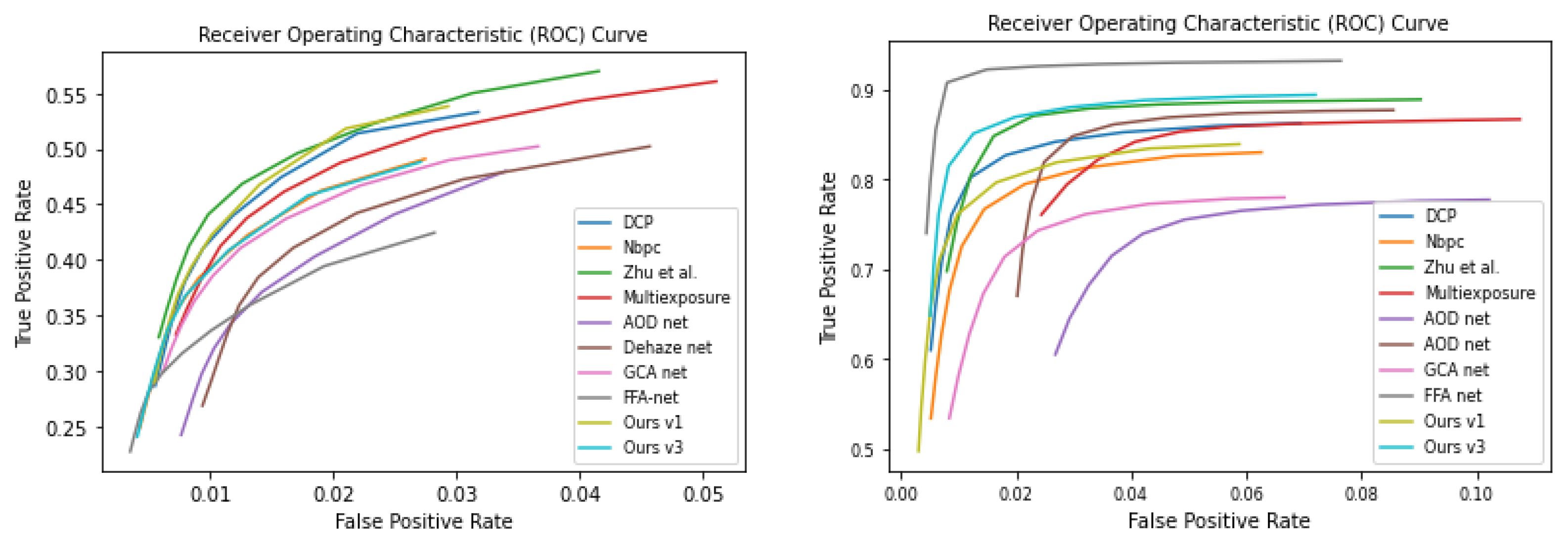
4.1. Quantitative Evaluation

4.1.1. Evaluation on Standard Metrics

Table 2. Comparison of the PSNR index on four datasets: fifty images from the FRIDA and the SOTS datasets and forty-five images from the NTIRE20 and the O-HAZE datasets. W corresponds to our main algorithm assuming white fog, and C is the color version (see Section 3.6), and I the interpolated version (see Section 3.5). The best results are in bold.

PSNR
Methods	FRIDA	SOTS	NTIRE20	O-HAZE
DCP [6]	12.26 (1.55)	18.91 (3.85)	12.77 (1.67)	16.95 (2.38)
NBPC [15]	11.59 (1.73)	18.07 (2.46)	12.24 (1.51)	15.85 (1.78)
Zhu et al. [12]	12.15 (1.77)	16.06 (2.74)	11.98 (1.67)	16.58 (2.53)
Zhu et al. [22]	11.93 (1.73)	19.13 (2.52)	13.29 (1.48)	16.81 (2.58)
AOD-Net [26]	10.73 (1.84)	19.39 (2.32)	11.98 (1.57)	15.04 (1.65)
Dehaze-Net [23]	10.87 (1.52)	23.41 (3.54)	12.33 (1.56)	15.41 (2.75)
GCA-Net [27]	12.79 (1.49)	22.68 (4.97)	12.82 (2.23)	16.43 (2.78)
FFA-Net [37]	10.38 (1.96)	34.10 (3.51)	12.40 (1.64)	16.19 (3.18)
W	12.62 (2.05)	18.40 (2.90)	13.16 (1.45)	17.02 (2.66)
C	12.27 (2.04)	16.77 (2.86)	13.90 (1.57)	18.32 (2.74)
I	11.65 (1.93)	24.40 (3.94)	12.69 (1.57)	16.57 (3.29)

and

Table 3. Comparison of the SSIM index on four datasets: fifty images from the FRIDA and the SOTS datasets, forty-five images from the NTIRE20 and the O-HAZE datasets. W corresponds to our main algorithm assuming white fog, C is the color version (see Section 3.6), and I the interpolated version (see Section 3.5). The best results are in bold.

SSIM
Methods	FRIDA	SOTS	NTIRE20	O-HAZE
DCP [6]	0.70 (0.06)	0.89 (0.06)	0.44 (0.10)	0.66 (0.10)
NBPC [15]	0.75 (0.07)	0.89 (0.03)	0.41 (0.09)	0.61 (0.09)
Zhu et al. [12]	0.72 (0.06)	0.88 (0.04)	0.45 (0.10)	0.66 (0.10)
Zhu et al. [22]	0.75 (0.06)	0.86 (0.07)	0.55 (0.09)	0.67 (0.10)
AOD-Net [26]	0.73 (0.07)	0.85 (0.05)	0.41 (0.09)	0.54 (0.01)
Dehaze-Net [23]	0.65 (0.07)	0.90 (0.09)	0.44 (0.10)	0.60 (0.10)
GCA-Net [27]	0.70 (0.08)	0.91 (0.06)	0.47 (0.10)	0.61 (0.10)
FFA-Net [37]	0.73 (0.08)	0.98 (0.01)	0.46 (0.10)	0.63 (0.10)
W	0.81 (0.07)	0.85 (0.08)	0.51 (0.09)	0.65 (0.11)
C	0.81 (0.07)	0.82 (0.08)	0.51 (0.09)	0.67 (0.11)
I	0.78 (0.07)	0.93 (0.05)	0.48 (0.09)	0.66 (0.12)

show that all methods are competitive, but our method (W) outperforms the others for both criteria on the FRIDA, NTIRE20, and O-HAZE datasets. On the O-HAZE dataset, the color version of our method (C) shows better performance. The color distortions are attenuated. The results on the SOTS dataset show that the proposed algorithm is less efficient on images where the veil is spatially close to uniform, as described in Section 3.5. Our method (I) allows for dealing with constant veils and provides better results on the SOTS dataset in terms of SSIM and PSNR. However, the performance decreases slightly on the three other databases compared to the two other versions of our method (W and C). The main result is that I generalizes to more types of fog. Then, the general performance of the interpolated method is higher than those of the other algorithms.

Table 4. Comparison of the FSIMc index on four datasets: fifty images from the FRIDA and the SOTS datasets, forty-five images from the NTIRE20 and the O-HAZE datasets. W corresponds to our main algorithm assuming white fog, and C is the color version (see Section 3.6), and I the interpolated version (see Section 3.5). The best results are in bold.

FSIMc
Methods	FRIDA	SOTS	NTIRE20	O-HAZE
DCP [6]	0.83 (0.06)	0.96 (0.02)	0.55 (0.07)	0.85 (0.06)
NBPC [15]	0.81 (0.06)	0.96 (0.01)	0.53 (0.06)	0.80 (0.08)
Zhu et al. [12]	0.82 (0.06)	0.96 (0.01)	0.55 (0.06)	0.82 (0.08)
Zhu et al. [22]	0.81 (0.06)	0.95 (0.02)	0.73 (0.05)	0.85 (0.08)
AOD-Net [26]	0.79 (0.06)	0.93 (0.02)	0.67 (0.06)	0.78 (0.08)
Dehaze-Net [23]	0.81 (0.06)	0.98 (0.01)	0.53 (0.07)	0.78 (0.09)
GCA-Net [27]	0.80 (0.05)	0.97 (0.02)	0.74 (0.06)	0.87 (0.06)
FFA-Net [37]	0.79 (0.06)	0.99 (0.004)	0.66 (0.07)	0.80 (0.09)
W	0.83 (0.06)	0.95 (0.02)	0.70 (0.06)	0.84 (0.07)
C	0.83 (0.06)	0.95 (0.02)	0.71 (0.06)	0.85 (0.07)
I	0.82 (0.06)	0.98 (0.01)	0.69 (0.06)	0.83 (0.08)

shows that our algorithms are competitive on the four datasets. The results obtained with the FSIMc metric contribute to illustrating the genericity of our method. In particular, Algorithm I competes with deep learning algorithms such as Dehaze-Net and FFA-Net on the SOTS dataset. On the FRIDA dataset, our method and the DCP method perform best. The GCA-Net and AOD-Net algorithms seem to outperform on the NTIRE20 datasets; however, the qualitative evaluation shows severe color distortions and darkenings. Our methods provide very good results on these two datasets. Moreover, the color version (C) of our algorithm seems to play a role in improving the performance on the O-haze and Ntire20 datasets. Indeed, the color version is better than the others to handling the blue-shift distortions.

4.1.2. Evaluation on Additional Metrics

PSNR, SSIM, and FSIMc are useful and broadly used criteria, but they are not sufficient to rate the quality of image restoration. Figure 10a gives an example where the restoration succeeds for objects in the background (see the arrow on the left), whereas the car in the foreground is degraded (arrow on the right). Conversely, the restoration in Figure 10b preserves the foreground but degrades the background. However, the results of the SSIM and PSNR metrics are approximately the same:

SSIM = 0.89 and PSNR = 17.9 (Figure 10a) and SSIM = 0.89 and PSNR = 17.7 (Figure 10b).

This example reveals that global quality indexes such as the PSNR, FSIMc, and SSIM may be inadequate either because the restoration is inefficient, or because the algorithm over-restores contrast in the areas where fog is absent or almost absent. In addition to these global metrics, we propose to estimate the quality of the restored images with two weight maps (Figure 10c,d), which are dense in areas where fog is respectively thick or thin.

Moreover, depending on the application, one may wish to preserve various features of the image. We have considered three important features in the following evaluation: image intensity, intensity of the gradient images, and image structure similarity (SSIM). In the following, the performance of the three proposed algorithms, named W (white fog), C (color), and I (interpolation), is compared with these new indexes (see Figure 11):

• d1: Weighted distance between the SSIM of the ground truth and the SSIM of the restored images (Figure 11a).
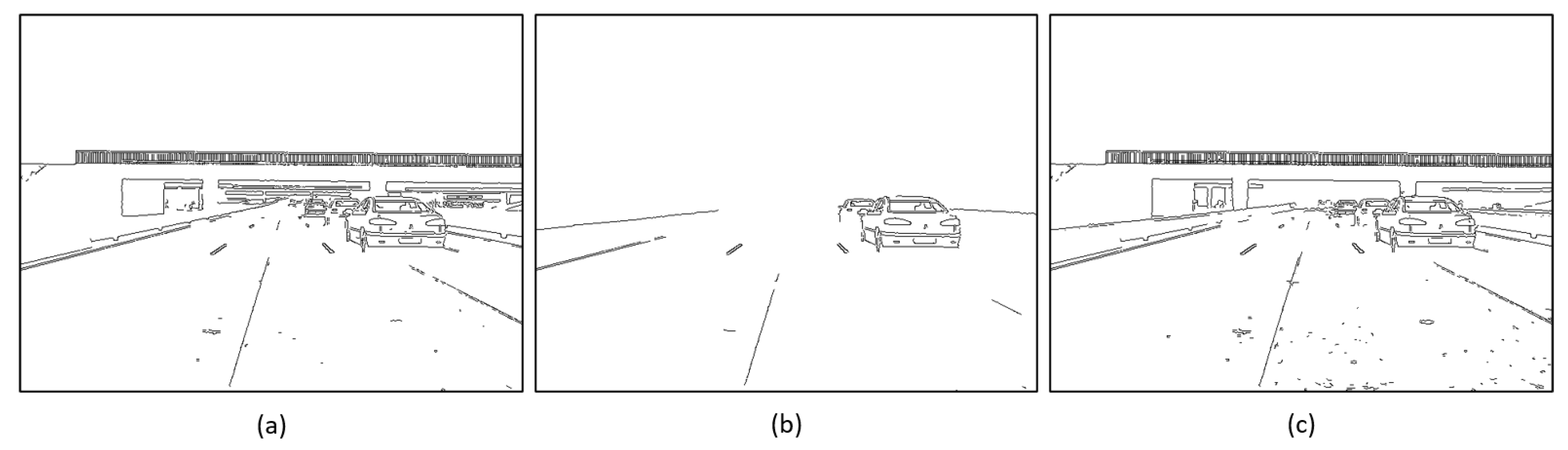
• d2: Weighted distance between the gradient of the ground truth and the gradient of the restored images (Figure 11b).
• d3: Weighted distance between the ground truth and the restored images (Figure 11c).

The weighted distance calculations are defined as:

$$\begin{array}{c}\hfill d_{Fog}=\frac{1}{p}\sum _{i=1}^{n}p(G_i-F{R}_i)\end{array}$$

(7a)

$$\begin{array}{c}\hfill d_{NoFog}=\frac{1}{(1-p)}\sum _{i=1}^n(1-p)(G_i-F{R}_i)\end{array}$$

(7b)

where p is a weight map roughly associated with foggy regions in the image (we use a normalized version of the pre-veil), G the ground truth, R the restored image, and F an intensity compensation factor between the restored image and the ground truth. $d_{NoFog}$ emphasizes the parts of the image close to the camera (Figure 10c), whereas $d_{Fog}$ emphasizes the foggy part (Figure 10d).

Table 5. Comparison of three distance indexes d1, d2 and d3 on fifty images from the SOTS dataset, with the $d_{Fog}$ index (in the fog area). W corresponds to our main algorithm assuming white fog, C to the color version, and I to the interpolation version. The two best results are in bold. The best result is also underlined.

${\mathit{d}}_{\mathit{Fog}}$
Methods	d1	d2	d3
DCP [6]	0.01 (0.05)	0.08 (0.003)	24.3 (8.6)
NBPC [15]	0.08 (0.02)	0.01 (0.003)	23.4 (10.8)
Zhu et al. [12]	0.60 (0.03)	0.05 (0.02)	67.7 (12.7)
Zhu et al. [22]	0.10 (0.05)	0.01 (0.004)	33.5 (15.8)
AOD-Net [26]	0.12 (0.04)	0.01 (0.003)	28.4 (16.6)
Dehaze-Net [23]	0.06 (0.05)	0.006 (0.002)	24.0 (15.6)
GCA-Net [27]	0.08 (0.04)	0.01 (0.004)	22.7 (15.6)
FFA-Net [37]	0.01 (0.005)	0.004 (0.001)	4.97 (2.3)
W (white fog)	0.10 (0.06)	0.009 (0.002)	42.0 (16.8)
C (color)	0.08 (0.06)	0.01(0.002)	30.3 (16.8)
I (interpolation)	0.04(0.03)	0.006(0.003)	23.5 (14.9)

and

Table 6. Comparison of three distance indexes d1, d2, and d3 on fifty images from the SOTS dataset, with the $d_{NoFog}$ index (in the no-fog area). W corresponds to our main algorithm assuming white fog, C to the color version, and I to the interpolation version. The two best results are in bold. The best result is also underlined.

${\mathit{d}}_{\mathit{NoFog}}$
Methods	d1	d2	d3
DCP [6]	0.09 (0.05)	0.01 (0.003)	16.4 (6.5)
NBPC [15]	0.10 (0.04)	0.01 (0.003)	15.0 (4.5)
Zhu et al. [12]	0.70 (0.05)	0.05 (0.002)	54.5 (5.25)
Zhu et al. [22]	0.15 (0.08)	0.02 (0.005)	19.8 (5.0)
AOD-Net [26]	0.20 (0.06)	0.02 (0.004)	18.7 (6.9)
Dehaze-Net [23]	0.12 (0.1)	0.007 (0.002)	14.8 (6.6)
GCA-Net [27]	0.11 (0.05)	0.01 (0.005)	15.4 (8.2)
FFA-Net [37]	0.01 (0.008)	0.005 (0.001)	4.40 (1.9)
W (white fog)	0.20 (0.1)	0.009 (0.003)	24.5 (5.7)
C (color)	0.11 (0.1)	0.01 (0.003)	18.8 (5.9)
I (interpolation)	0.08 (0.06)	0.006 (0.002)	14.2 (6.1)

show that the Interpolation method outperforms the W and C versions, as expected, on the SOTS dataset (since these are distance calculations, smaller values are better). It provides good results on the three proposed metrics, and it is competitive with previous algorithms, both model-based and learning-based.

In addition to these metrics, an edge-based criterion was considered. It consists of applying an edge filter, such as the Canny edge detector [41], on both the ground truth and the restored images, and to compare the two binary edge maps in order to assess the benefit of restoration in terms of edge visibility. This criteria may be useful, for instance, to assess restoration for detection algorithms for onboard cameras. Figure 12 shows that edge maps obtained with the Canny filter on the same scene without fog, with fog, and after fog removal.

The two binary edge maps are compared with a Receiver Operating Characteristic (ROC), varying the min threshold between 0 and the max threshold value (Figure 13). The left image on Figure 13 shows that Zhu et al. [12], our W algorithm, the DCP, and the multi-exposure method [22] perform better than the other in terms of edge visibility restoration. Our Interpolation algorithm, the NBPC, and the GCA-Net are also competitive in terms of edges restoration, with lower performances. The best rated algorithm tends to succeed better in restoring edges at large distances.

The right image in Figure 13 shows that, while FFA-net outperforms others in terms of edge visibility on the SOTS dataset, it gives the worst results on the FRIDA dataset. This algorithm has been trained to be very efficient on images with a spatially uniform veil (as in the RESIDE/SOTS datasets). The quantitative evaluation shows it does not generalize to different types of fog, which is the goal of ours. After FFA-net, our Interpolation algorithm and Zhu et al. [12] provide very good results, whereas DCP and Dehaze-Net are competitive on the SOTS dataset. Our White fog algorithm gives better results in terms of edge visibility than the Interpolation version on the FRIDA dataset, whereas it is the opposite on the SOTS dataset. This strengthens the idea that the Interpolation version gives better results with spatially uniform fog.

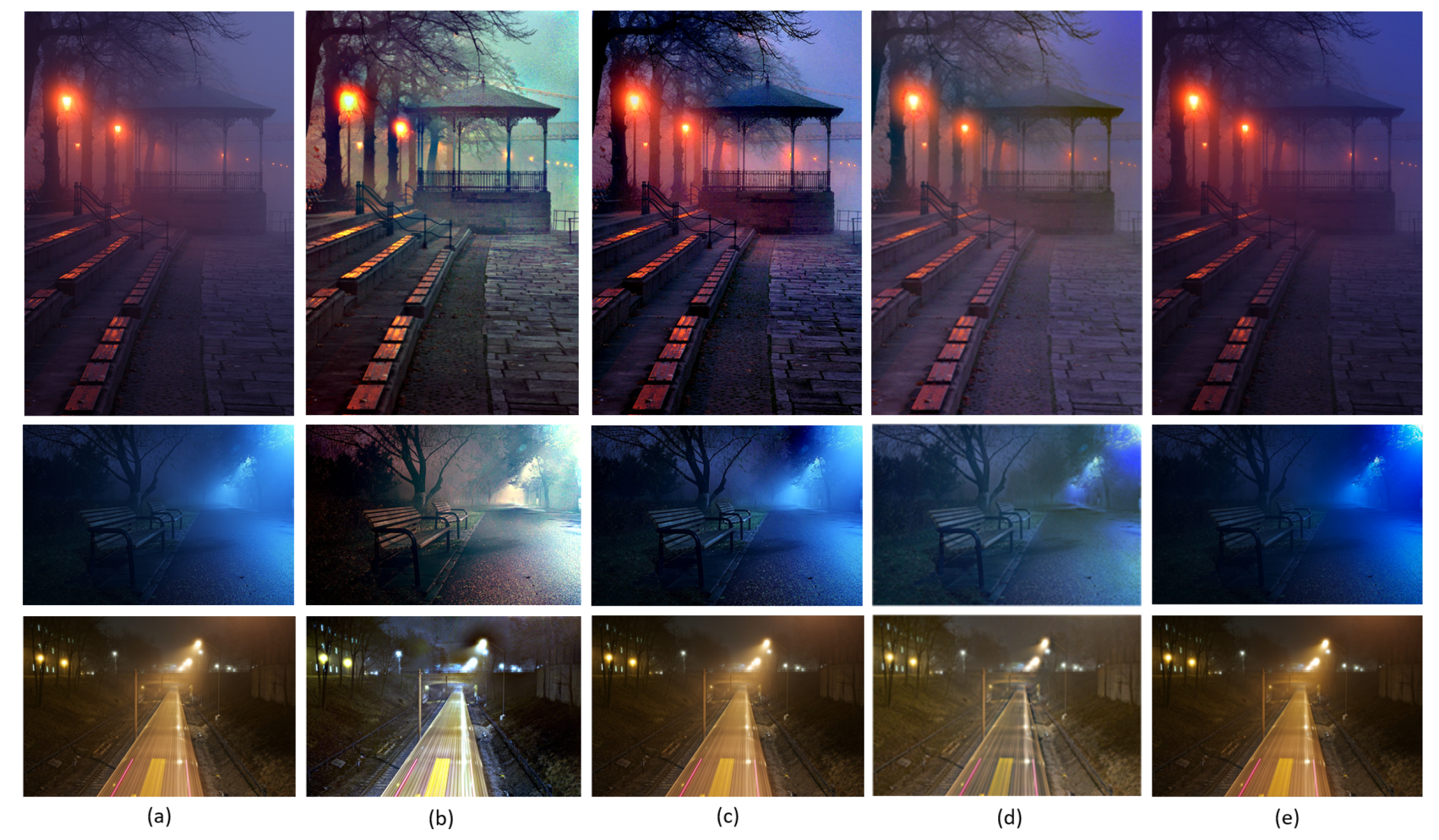
4.2. Qualitative Evaluation

Real world images from previous works on single image fog removal have been used for a qualitative comparison. DCP, NBPC, and Zhu et al. [12] algorithms remove the fog with good results (Figure 14). However, DCP images are bright and contrasted, whereas NBPC and Zhu et al.’s [12] results are darker and more faded. Zhu et al.’s [22] method provides very contrasted and saturated results, particularly notable in the pumpkins and the mountain images. The AOD-Net learning-based method provides faded and dark results but with less halos. It appears in the tree and the buildings images that the Dehaze-Net method retains far away haze. It works better with colored sky regions, avoiding artifacts and blue-shift distortions found with most algorithms. FFA-Net seems to retain far away haze more than Dehaze-Net. This effect is particularly significant in the images with sky regions as in the tree and the building images. GCA-Net produces artifacts in the sky of the tree image and of the the first two lines images but provides good and colored results in other images. The White fog version of our algorithm provides light images and removes the haze over the entire images. The color version reduces color distortions.

Figure 15 shows results on images from the O-HAZE dataset with two versions of our algorithm. The results of the White fog version of the algorithm (Figure 15c) are blue-shifted and noisy. The color version of the algorithm succeeds in attenuating the blue-shift effect (see Figure 15d) and contributes to improving the criterion described in Section 4.1.

4.3. Robustness of the Proposed Algorithm

Figure 16 shows sample results of our algorithm on nighttime images. To test the relevance of our algorithm for nighttime images, a comparison was conducted with two state-of-the-art algorithms, Li et al. [31] and Yu et al. [42], on previously used nighttime images. Figure 16 shows that the algorithm of Li et al. succeeds in attenuating halos, but the images are color-shifted and noisy, particularly in sky regions. On the contrary, the algorithm of Yu et al. produces light and contrasted images with color consistency and natural rendering, whereas halos seem emphasized, particularly in the bottom part of the image. The color version of our algorithm succeeds in attenuating halos and maintaining a natural color rendering. It is particularly notable in the bottom part of the image; in the top part of the image, the objects far away are not contrasted enough.

Figure 17 shows a comparison between the white version (W) and the colored version (C) of our algorithm of an image representing a halo with an orange fog. Figure 17b shows that W seems to accentuate the glow effect and does not remove the colored fog. In contrast, C (Figure 17c) succeeds in attenuating the halo effect and the orange shift. The histogram in Figure 17d shows the intensity distribution of the image. The blue part corresponds to the input foggy image. It is evenly distributed over the intensity range [0.2, 1.0], which represents the foggy part of the image. Therefore, ideally, the histogram of the restored image should peak towards the left side of the histogram.

Figure 18 shows a comparison between the colored version (C) of our algorithm and the two other algorithms of the state-of-the-art mentioned in Figure 16. Figure 18b shows that Li et al.’s result succeeds in eliminating the glow effect, but introduces color distortions. Yu et al.’s result (Figure 18c) seems to slightly attenuate the colored fog. However, the histogram distribution (the yellow part) shows that the fog around the artificial source is not completely removed. A peak in the left side of the histogram seems to be a good indicator of night fog removal (Our C and Li et al. [31]).

Table 7. Comparison of the SSIM and PSNR indexes on twenty synthetic nighttime images.

Methods	SSIM	PSNR
Yu et al. [42]	0.62	13.39
Li et al. [31]	0.61	12.59
C (color)	0.60	11.33

shows a small quantitative evaluation on a database of twenty synthetic nighttime images created by Zhang et al. [43] from the Middlebury dataset (see an example in Figure 19). The results show that our method is slightly lower but remains competitive with methods dedicated to nighttime image restoration. It also shows that the simple method of applying our idea on each color channel gives promising results.

Figure 20 illustrates that applying our algorithm on each color channel may also be promising for underwater visibility restoration.

5. Discussion

We have reinterpreted the DCP method in terms of three priors. We propose to improve the third prior, associated with $\omega$, with a smooth modulation function as a prior to estimate the atmospheric veil from the pre-veil. The input parameters of this function are automatically estimated according to the input image pixel intensities in light (sky) and dark (ground) regions, after filtering. In addition, our method makes it possible to generalize to different types of fog, both depth-dependent fog and spatially uniform fog. The evaluation on the different databases with different types of fog testifies to the generalizability of our algorithm. The proposed method provides good results on both synthetic and real world images for objects at all distances. To extend the proposed algorithm to smoke, dust, and other colored airborne particles, we process each color channel separately, in order to remove colored components. This allows for applying the algorithm to nighttime images as well as underwater images. An interpolation is needed between our Naka–Rushton algorithm and a constant veil algorithm in order to cope with images with a more or less uniform veiling luminance. The proposed algorithms should be carefully evaluated for various applications in daylight, nighttime, and possibly underwater.

References

1. Tremblay, M.; Halder, S.; De Charette, R.; Lalonde, J.F. Rain Rendering for Evaluating and Improving Robustness to Bad Weather. Int. J. Comput. Vis. Vol. 2020, 129, 341–360. [Google Scholar] [CrossRef]
2. Huang, S.C.; Le, T.H.; Jaw, D.W. DSNet: Joint Semantic Learning for Object Detection in Inclement Weather Conditions. IEEE Trans. Pattern Anal. Mach. Intell. 2020, 1. [Google Scholar] [CrossRef]
3. Hautière, N.; Tarel, J.P.; Aubert, D. Towards Fog-Free In-Vehicle Vision Systems through Contrast Restoration. In Proceedings of the 2007 IEEE Conference on Computer Vision and Pattern Recognition (CVPR), Minneapolis, MN, USA, 17–22 June 2007; pp. 1–8. [Google Scholar]
4. Duminil, A.; Tarel, J.P.; Brémond, R. Single Image Atmospheric Veil Removal Using New Priors. In Proceedings of the 2021 IEEE International Conference on Image Processing (ICIP), Anchorage, AK, USA, 19–22 September 2021. [Google Scholar]
5. He, K.; Sun, J.; Tang, X. Single image haze removal using dark channel prior. In Proceedings of the 2009 IEEE Conference on Computer Vision and Pattern Recognition (CVPR), Miami, FL, USA, 20–25 June 2009; pp. 1956–1963. [Google Scholar]
6. He, K.; Sun, J.; Tang, X. Single Image Haze Removal Using Dark Channel Prior. IEEE Trans. Pattern Anal. Mach. Intell. 2011, 33, 2341–2353. [Google Scholar] [CrossRef]
7. He, K.; Sun, J.; Tang, X. Guided image filtering. In Proceedings of the 2010 European Conference on Computer Vision (ECCV), Crete, Greece, 5–11 September 2010; pp. 1–14. [Google Scholar]
8. Caraffa, L.; Tarel, J.P.; Charbonnier, P. The Guided Bilateral Filter: When the Joint/Cross Bilateral Filter Becomes Robust. IEEE Trans. Image Process. 2015, 24, 1199–1208. [Google Scholar] [CrossRef] [Green Version]
9. Xu, H.; Guo, J.; Liu, Q.; Ye, L. Fast image dehazing using improved dark channel prior. In Proceedings of the 2012 IEEE International Conference on Information Science and Technology, Wuhan, China, 23–25 March 2012; pp. 663–667. [Google Scholar] [CrossRef]
10. Meng, G.; Wang, Y.; Duan, J.; Xiang, S.; Pan, C. Efficient Image Dehazing with Boundary Constraint and Contextual Regularization. In Proceedings of the 2013 IEEE International Conference on Computer Vision, Sydney, NSW, Australia, 1–8 December 2013; pp. 617–624. [Google Scholar] [CrossRef]
11. Li, Z.; Zheng, J. Edge-Preserving Decomposition-Based Single Image Haze Removal. IEEE Trans. Image Process. 2015, 24, 5432–5441. [Google Scholar] [CrossRef]
12. Zhu, M.; He, B.; Wu, Q. Single Image Dehazing Based on Dark Channel Prior and Energy Minimization. IEEE Signal Process. Lett. 2018, 25, 174–178. [Google Scholar] [CrossRef]
13. Jackson, J.; Kun, S.; Agyekum, K.O.; Oluwasanmi, A.; Suwansrikham, P. A Fast Single-Image Dehazing Algorithm Based on Dark Channel Prior and Rayleigh Scattering. IEEE Access 2020, 8, 73330–73339. [Google Scholar] [CrossRef]
14. Zhang, C.; Zhang, Y.; Lu, J. Single image dehazing using a novel criterion based segmenting dark channel prior. In Proceedings of the 2019 Eleventh International Conference on Graphics and Image Processing (ICGIP); Pan, Z., Wang, X., Eds.; SPIE: Hangzhou, China, 2020; p. 121. [Google Scholar] [CrossRef]
15. Tarel, J.P.; Hautiere, N. Fast visibility restoration from a single color or gray level image. In Proceedings of the 2009 IEEE 12th International Conference on Computer Vision (ICCV), Kyoto, Japan, 29 September–2 October 2009; pp. 2201–2208. [Google Scholar] [CrossRef]
16. Tarel, J.P.; Hautiere, N.; Caraffa, L.; Cord, A.; Halmaoui, H.; Gruyer, D. Vision Enhancement in Homogeneous and Heterogeneous Fog. IEEE Intell. Transp. Syst. Mag. 2012, 4, 6–20. [Google Scholar] [CrossRef] [Green Version]
17. Negru, M.; Nedevschi, S.; Peter, R.I. Exponential Contrast Restoration in Fog Conditions for Driving Assistance. IEEE Trans. Intell. Transp. Syst. 2015, 16, 2257–2268. [Google Scholar] [CrossRef]
18. Ancuti, C.O.; Ancuti, C.; Bekaert, P. Effective single image dehazing by fusion. In Proceedings of the 2010 IEEE International Conference on Image Processing (ICIP), Hong Kong, China, 26–29 September 2010; pp. 3541–3544. [Google Scholar] [CrossRef]
19. Ancuti, C.O.; Ancuti, C. Single Image Dehazing by Multi-Scale Fusion. IEEE Trans. Image Process. 2013, 22, 3271–3282. [Google Scholar] [CrossRef]
20. Wang, Q.; Zhao, L.; Tang, G.; Zhao, H.; Zhang, X. Single-Image Dehazing Using Color Attenuation Prior Based on Haze-Lines. In Proceedings of the 2019 IEEE International Conference on Big Data (Big Data), Los Angeles, CA, USA, 9–12 December 2019; pp. 5080–5087. [Google Scholar] [CrossRef]
21. Zheng, M.; Qi, G.; Zhu, Z.; Li, Y.; Wei, H.; Liu, Y. Image Dehazing by an Artificial Image Fusion Method Based on Adaptive Structure Decomposition. IEEE Sens. J. 2020, 20, 8062–8072. [Google Scholar] [CrossRef]
22. Zhu, Z.; Wei, H.; Hu, G.; Li, Y.; Qi, G.; Mazur, N. A Novel Fast Single Image Dehazing Algorithm Based on Artificial Multiexposure Image Fusion. IEEE Trans. Instrum. Meas. 2021, 70, 1–23. [Google Scholar] [CrossRef]
23. Cai, B.; Xu, X.; Jia, K.; Qing, C.; Tao, D. DehazeNet: An End-to-End System for Single Image Haze Removal. IEEE Trans. Image Process. 2016, 25, 5187–5198. [Google Scholar] [CrossRef] [PubMed] [Green Version]
24. Ren, W.; Liu, S.; Zhang, H.; Pan, J.; Cao, X.; Yang, M.H. Single Image Dehazing via Multi-scale Convolutional Neural Networks. In Computer Vision—ECCV 2016; Leibe, B., Matas, J., Sebe, N., Welling, M., Eds.; Lecture Notes in Computer Science; Springer International Publishing: Cham, Switzerland, 2016; pp. 154–169. [Google Scholar] [CrossRef]
25. Meinhardt, T.; Moeller, M.; Hazirbas, C.; Cremers, D. Learning Proximal Operators: Using Denoising Networks for Regularizing Inverse Imaging Problems. In Proceedings of the 2017 IEEE International Conference on Computer Vision (ICCV), Venice, Italy, 22–29 October 2017; pp. 1799–1808. [Google Scholar] [CrossRef] [Green Version]
26. Li, B.; Peng, X.; Wang, Z.; Xu, J.; Feng, D. An All-in-One Network for Dehazing and Beyond. arXiv 2017, arXiv:1707.06543. [Google Scholar]
27. Chen, D.; He, M.; Fan, Q.; Liao, J.; Zhang, L.; Hou, D.; Yuan, L.; Hua, G. Gated Context Aggregation Network for Image Dehazing and Deraining. In Proceedings of the 2019 IEEE Winter Conference on Applications of Computer Vision (WACV), Waikoloa Village, HI, USA, 7–11 January 2019; pp. 1375–1383. [Google Scholar] [CrossRef] [Green Version]
28. Engin, D.; Genc, A.; Ekenel, H.K. Cycle-Dehaze: Enhanced CycleGAN for Single Image Dehazing. In Proceedings of the 2018 IEEE/CVF Conference on Computer Vision and Pattern Recognition Workshops (CVPRW), Salt Lake City, UT, USA, 18–22 June 2018; pp. 938–9388. [Google Scholar] [CrossRef] [Green Version]
29. Zhu, H.; Peng, X.; Chandrasekhar, V.; Li, L.; Lim, J.H. DehazeGAN: When Image Dehazing Meets Differential Programming. In Proceedings of the Twenty-Seventh International Joint Conference on Artificial Intelligence (IJCAI-18), Stockholm, Sweden, 13–19 July 2018; p. 7. [Google Scholar]
30. Naka, K.I.; Rushton, W.A.H. S-potentials from color units in the retina of fish (Cyprinidae). J. Physiol. 1966, 185. [Google Scholar] [CrossRef]
31. Li, Y.; Tan, R.T.; Brown, M.S. Nighttime Haze Removal with Glow and Multiple Light Colors. In Proceedings of the 2015 IEEE International Conference on Computer Vision (ICCV), Santiago, Chile, 7–13 December 2015; pp. 226–234. [Google Scholar] [CrossRef]
32. Ancuti, C.; Ancuti, C.O.; De Vleeschouwer, C.; Bovik, A.C. Night-time dehazing by fusion. In Proceedings of the 2016 IEEE International Conference on Image Processing (ICIP), Phoenix, AZ, USA, 25–28 September 2016; pp. 2256–2260. [Google Scholar] [CrossRef]
33. Zhang, J.; Cao, Y.; Fang, S.; Kang, Y.; Chen, C.W. Fast Haze Removal for Nighttime Image Using Maximum Reflectance Prior. In Proceedings of the 2017 IEEE Conference on Computer Vision and Pattern Recognition (CVPR), Honolulu, HI, USA, 21–26 July 2017; pp. 7016–7024. [Google Scholar] [CrossRef]
34. Lou, W.; Li, Y.; Yang, G.; Chen, C.; Yang, H.; Yu, T. Integrating Haze Density Features for Fast Nighttime Image Dehazing. IEEE Access 2020, 8, 113318–113330. [Google Scholar] [CrossRef]
35. Petzold, D. What the Fog-Street Photography by Mark Broyer. WE AND THE COLOR. 2017. Available online: https://weandthecolor.com/what-the-fog-street-photography-mark-broyer/92328 (accessed on 29 April 2021).
36. Li, B.; Ren, W.; Fu, D.; Tao, D.; Feng, D.; Zeng, W.; Wang, Z. Benchmarking Single-Image Dehazing and Beyond. IEEE Trans. Image Process. 2019, 28, 492–505. [Google Scholar] [CrossRef] [PubMed] [Green Version]
37. Qin, X.; Wang, Z.; Bai, Y.; Xie, X.; Jia, H. FFA-Net: Feature Fusion Attention Network for Single Image Dehazing. Proc. AAAI Conf. Artif. Intell. 2020, 34, 11908–11915. [Google Scholar] [CrossRef]
38. Wang, Z.; Bovik, A.; Sheikh, H.; Simoncelli, E. Image Quality Assessment: From Error Visibility to Structural Similarity. IEEE Trans. Image Process. 2004, 13, 600–612. [Google Scholar] [CrossRef] [Green Version]
39. Zhang, L.; Zhang, L.; Mou, X.; Zhang, D. FSIM: A Feature Similarity Index for Image Quality Assessment. IEEE Trans. Image Process. 2011, 20, 2378–2386. [Google Scholar] [CrossRef] [Green Version]
40. Ancuti, C.O.; Ancuti, C.; Timofte, R.; De Vleeschouwer, C. O-HAZE: A Dehazing Benchmark With Real Hazy and Haze-Free Outdoor Images. In Proceedings of the 2018 IEEE/CVF Conference on Computer Vision and Pattern Recognition Workshops (CVPRW), Salt Lake City, UT, USA, 18–22 June 2018; pp. 754–762. [Google Scholar]
41. Canny, J. A Computational Approach to Edge Detection. IEEE Trans. Pattern Anal. Mach. Intell. 1986, 8, 679–698. [Google Scholar] [CrossRef] [PubMed]
42. Yu, T.; Song, K.; Miao, P.; Yang, G.; Yang, H.; Chen, C. Nighttime Single Image Dehazing via Pixel-Wise Alpha Blending. IEEE Access 2019, 7, 114619–114630. [Google Scholar] [CrossRef]
43. Zhang, J.; Cao, Y.; Zha, Z.J.; Tao, D. Nighttime Dehazing with a Synthetic Benchmark. In Proceedings of the 28th ACM International Conference on Multimedia (ICM), Seattle, WA, USA, 12–16 October 2020; pp. 2355–2363. [Google Scholar]
44. Hirschmüller, H.; Scharstein, D. Evaluation of cost functions for stereo matching. In Proceedings of the IEEE Computer Society Conference on Computer Vision and Pattern Recognition (CVPR 2007), Minneapolis, MN, USA, 17–22 June 2007. [Google Scholar]
45. Wang, Y.; Song, W.; Fortino, G.; Qi, L.Z.; Zhang, W.; Liotta, A. An Experimental-Based Review of Image Enhancement and Image Restoration Methods for Underwater Imaging. IEEE Access 2019, 7, 140233–140251. [Google Scholar] [CrossRef]
Figure 1. Flowchart of the proposed algorithm.
Atmosphere 12 00772 g001
Figure 2. Histograms showing the link between pre-veil and veil pixel intensities (mean of fifty images from the FRIDA dataset [16]). (a) homogeneous fog and illumination, (b) homogeneous fog and heterogeneous illumination, (c) heterogeneous fog and homogeneous illumination, (d) heterogeneous fog and illumination.
Atmosphere 12 00772 g002
Figure 3. Foggy pixels and veil pixels intensities: (a) histogram showing the link between pre-veil and veil pixel intensities (mean of fifty images from the FRIDA dataset [16]), (b) input foggy image.
Atmosphere 12 00772 g003
Figure 4. (Left): the Naka–Rushton function with parameters R m a x , K and n. (Right): the modulation function, shaped like the left-hand side of the Naka–Rushton function, showing parameters I s , I 0 and ϵ .
Atmosphere 12 00772 g004
Figure 5. Estimating I s and I 0 : (a) input image, (b) filtered image using a morphological opening, (c) pixels where the intensity is maximum, (d) pixels where the intensity is minimum.
Atmosphere 12 00772 g005
Figure 6. Atmospheric veil estimation from the morphologically filtered pre-veil using Naka–Rushton as a modulation function.
Atmosphere 12 00772 g006
Figure 7. Nighttime foggy images. Reprinted with permission from ref. [35]. Copyright 2021 Mark Broyer.
Atmosphere 12 00772 g007
Figure 8. RGB values comparison: (a) daylight white fog image from the RESIDE dataset [36], (b) histogram of the daylight white fog image, (c) colored fog image (reprinted with permission from ref. [35]. Copyright 2021 Mark Broyer), (d) histogram of the colored fog image. This figure shows the RGB values of the pixel in the center of the black squares. Pixel intensity is between 0 and 255.
Atmosphere 12 00772 g008
Figure 9. Atmospheric veils before the refinement step: (a) atmospheric veil estimation of a white fog image, (b) atmospheric veil estimation of a colored foggy image from the color channel with the minimum intensity, (c) atmospheric veil estimation of a colored foggy image from each color channel (adapted with permission from ref. [35]. Copyright 2021 Mark Broyer).
Atmosphere 12 00772 g009
Figure 10. FRIDA images: (a) restored image; SSIM = 0.89 and PSNR = 17.9; (b) restored image; SSIM = 0.89, PSNR = 17.7, (c) weight map focusing on the bottom part of the input foggy image, and (d) weight map focusing on the foggy part of the input foggy image.
Atmosphere 12 00772 g010
Figure 11. (a) SSIM map of a restored image from the FRIDA dataset, (b) gradient map, (c) intensity map.
Atmosphere 12 00772 g011
Figure 12. Edge maps after application of the Canny filter on a FRIDA image: (a) without fog, (b) with fog, (c) after restoration. The min and max thresholds of the edge detector are set to 120 and 180.
Atmosphere 12 00772 g012
Figure 13. ROC curves comparison for different algorithms. (Left): ROC curves obtained from fifty images of the FRIDA dataset. (Right): ROC curve from fifty images of the SOTS dataset. The max threshold of the Canny filter is set to 180. The legend Multiexposure corresponds to Zhu et al.’s [22] method.
Atmosphere 12 00772 g013
Figure 14. Comparison of fog removal results on real world images: (a) input foggy images, (b) DCP [6], (c) NBPC [15], (d) Zhu et al. [12], (e) Zhu et al. [22], (f) Dehaze-Net [23] (g) AOD-Net [26], (h) GCA-Net [27], (i) FFA-Net [37], (j) White fog, and (k) Color algorithm.
Atmosphere 12 00772 g014
Figure 15. O-HAZE images [40]: (a) without fog, (b) with fog, (c) images restored with the White fog version of our algorithm (W), (d) images restored with the color version of our algorithm (C).
Atmosphere 12 00772 g015
Figure 16. Comparison on nighttime images from [33]: (a) foggy images, (b) Li et al. [31], (c) Yu et al. [42], (d) color version (C), (e) white version (W).
Atmosphere 12 00772 g016
Figure 17. Comparison on a glow patch: (a) input foggy image, (b) restored patch with our white fog algorithm, (c) restored patch with our colored fog algorithm, (d) histogram of the intensity of each glow patch (glow images are Reprinted with permission from ref. [35]. Copyright 2021 Mark Broyer).
Atmosphere 12 00772 g017
Figure 18. Comparison on a glow patch: (a) foggy image, (b) Li et al. [31], (c) Yu et al. [42], (d) restored image with the color version of our algorithm, (e) histogram of the intensity of each glow patch (glow images are adapted with permission from ref. [35]. Copyright 2021 Mark Broyer).
Atmosphere 12 00772 g018
Figure 19. Image from the Middlebury dataset [44]: (a) input image, (b) nighttime synthetic image [43]. In the context of synthetic images, the size of the opening filter is set to (30,30) instead of (10,10).
Atmosphere 12 00772 g019
Figure 20. Underwater images from [45]: (a) input images, (b) images restored with our White fog algorithm (W), (c) images restored with the color version of our algorithm (C).
Atmosphere 12 00772 g020