Article

Can a Warm Ocean Feature Cause a Typhoon to Intensify Rapidly?

1
IHOS, National Central University, Taoyuan 32001, Taiwan
2
Forrestal Campus, Princeton University, Princeton, NJ 08544, USA
3
Atmospheric Sciences, Chinese Cultural University, Taipei 11114, Taiwan
*
Authors to whom correspondence should be addressed.
Atmosphere 2021, 12(6), 797; https://doi.org/10.3390/atmos12060797
Submission received: 15 May 2021 / Revised: 10 June 2021 / Accepted: 15 June 2021 / Published: 21 June 2021
(This article belongs to the Special Issue Rapid Intensity Changes of Tropical Cyclones)

Abstract

:
The hypothesis that a warm ocean feature (WOF) such as a warm eddy may cause a passing typhoon to undergo rapid intensification (RI), that is, the storm’s maximum 1-min wind speed at 10-m height increases by more than 15.4 m/s in 1 day, is of interest to forecasters. Testing the hypothesis is a challenge, however. Besides the storm’s internal dynamics, typhoon intensity depends on other environmental factors such as vertical wind shear and storm translation. Here we designed numerical experiments that exclude these other factors, retaining only the WOF’s influence on the storm’s intensity change. We use a storm’s translation speed Uh = 5 m/s when surface cooling is predominantly due to 1D vertical mixing. Observations have shown that the vast majority (70%) of RI events occur in storms that translate between 3 to 7 m/s. We conducted a large ensemble of twin experiments with and without ocean feedback and with and without the WOF to estimate model uncertainty due to internal variability. The results show that the WOF increases surface enthalpy flux and moisture convergence in the storm’s core, resulting in stronger updrafts and intensity. However, the intensification rate is, in general, insufficiently rapid. Consequently, the number of RIs is not statistically significantly different between simulations with and without the WOF. An analytical coupled model supports the numerical findings. Furthermore, it shows that WOF-induced RI can develop only over eddies and ambient waters that are a few °C warmer than presently observed in the ocean.

1. Introduction

We follow Kaplan and DeMaria [1] to define typhoon or tropical cyclone rapid intensification (RI) when the storm’s maximum 1-min wind speed at 10-m height increases by more than 15.4 m/s in 1 day. Typhoons that undergo RI at least once in their lifetime are often significant storms of Category 3 and above [1,2,3]. They are potentially dangerous when the RI occurs just before the storm makes landfall. Two infamous examples are Hurricane Katrina (2005) in the Gulf of Mexico and Typhoon Haiyan (2013) in the Philippine Sea (120°–155° and 2° N–35° N). Both cost thousands of lives and hundreds of billions of dollars.
An ocean’s warm feature (WOF) may trigger RI as the storm passes [4,5,6,7,8]. We shall call this the WOF-RI hypothesis. Here, a WOF has a finite horizontal extent of several hundred kilometres. Its warm layer measured from the surface to the 26 °C isotherm, the Z26, exceeds 60 m: Z26 ≳ 60 m [9]. Examples include the Kuroshio and warm mesoscale eddies [10,11]. The definition also applies to summertime shallow continental shelf water with temperature everywhere warmer than 26 °C [8,12]. The idea is as follows. Because of the thicker Z26, the sea surface temperature (SST) in a WOF would not be readily cooled below 26 °C by the typhoon wind through mixing and upwelling. As a result, the water temperature remains above 26 °C and warmer than the surrounding sea outside the WOF. The WOF may then ‘boost’ the surface enthalpy flux as the storm passes, increases the potential intensity [13] of the storm, and may cause it to intensify rapidly.
Besides internal dynamics, the RI process also depends on external factors other than the WOF, such as the environmental vertical wind shear and storm’s translation [14,15,16,17,18,19,20]. The influence of WOF and other factors are implicit in observational and model data. Therefore, testing the WOF-RI hypothesis is challenging since these other factors need to be removed from the data to isolate the WOF’s influence. A recent analysis of global observations did not indicate a statistically significant relationship between RI and WOF, most probably because of the different factors in the observations [21].
On the other hand, testing the WOF-RI hypothesis is of interest. It may deepen our understanding of the RI process and improve the intensity forecast. It is well-accepted in the scientific community that one can more accurately forecast typhoon tracks than intensity [22]. Although a WOF continuously evolves, the evolution is, in most cases, sufficiently slow compared to the faster time scale taken for a storm to translate across it. The WOF is then approximately ‘frozen’ at the state before the storm [23]. Therefore, since WOFs in the open ocean appear as locally elevated sea-surface height anomalies on satellite altimetry maps, the locations and timings of potential RI events may be identified by laying the forecast storm track on the map. Studies have shown that the forecast of intensity changes is improved by including WOFs in the forecast [19,24,25].
In this study, we test the WOF-RI hypothesis by designing a model that isolates the influence of WOF on intensification. We then conduct experiments with and without the WOF inserted in the model and estimate the model spread due to internal dynamics using a large model ensemble. The results show that while an ocean’s WOF can cause a passing typhoon to intensify, it also induces increased storm asymmetry and cooling due to ocean feedback. Both factors reduce the rate of intensification. Consequently, the simulations that include WOF do not yield a statistically significant difference in RI events than those without the WFM. A simple analytical model with ocean feedback supports the numerical fining.

2. Methods

2.1. The Problem of Testing the WOF-RI Hypothesis

Our goal is to design a model that retains WOF as the only external environmental influence on typhoon intensity change. Consider a typhoon translating from east to west at the uniform speed Uh over a WOF. To accomplish uniform translation in the model, one usually specifies a constant steering flow. However, steering flow induces azimuthal asymmetry in the storm, which modifies intensity [16,26,27]. A variable Coriolis parameter (f, the β-effect) also induces asymmetry and modifies intensity; moreover, it generates intensity-dependent storm movement [16,28]. These effects would make the task of maintaining uniform translation and isolating the storm’s response to the WOF difficult. Therefore, we set steering flow and β to zero. We let the typhoon be stationary and instead let the WOF translate from west to east under the storm. Here, the WOF is an initially axisymmetric warm eddy. The typhoon sees and responds to a changing SST field as the warm eddy, which also evolves as the storm acts on it, approaches from the west, passes under the storm and leaves to the east (Figure 1). The model result then would support the WOF-RI hypothesis if it passes the following two-step test:
(1)
The warm eddy triggers RI while there is no RI in an otherwise identical model run without the warm eddy;
(2)
The number of RI events in a large ensemble of the model run with the warm eddy is statistically significantly more than the RI events for the corresponding twin runs without the warm eddy.

2.2. Modelling Strategy

We use an f-plane model (f = 5 × 10⁻⁵ s−1 at 20° N) with zero steering flow, and the typhoon remains nearly stationary. The typhoon centre (where the sea-level pressure SLP is minimum) wobbles slightly about its initial point during the model integration, about ± 20 km. However, that is small compared to the typical eddy diameter of ~300 km. We then make the warm eddy translate from west to east under the storm. The coding is straightforward when the model typhoon and warm eddy do not interact, in the limit of Z26 → ∞. In this case, there is no ocean feedback, and we can kinematically translate the eddy. In general finite Z26, we may translate the eddy by specifying a free-stream flow. However, this would produce a secondary circulation due to eddy-mean flow interaction unrelated to and complicating the RI-WOF problem. Therefore, we simplify the ocean model to consist merely of one-dimensional ocean columns [29,30,31,32]. The typhoon and ocean interact through exchanges of surface momentum and enthalpy fluxes. Such one-dimensional ocean approximation is widely used in coupled tropical cyclone-ocean simulations [5,33]. Emanuel [33] obtained highly accurate intensity predictions using such an approximation. As horizontal gradients are nil, the eddy cannot self-advect [30,31,32]. We can, again, kinematically translate the eddy. We exchange variables every 1 h by feeding a moving SST to the atmospheric grid and moving surface fluxes to the ocean grid. Ocean velocities are neglected in the exchange as they are much smaller than the typhoon wind.

2.3. The Atmosphere and Ocean Models

We use the Weather Research and Forecast (WRF) [34] model for the typhoon and the Princeton Ocean Model (POM) [31,35,36,37] for the ocean.
The WRF domain is 3000 km × 3000 km × 25 km, periodic in x (’zonal’) and y (’latitudinal’). The model’s initial vortex and spin-up follow Rotunno and Emanuel [38], also used in [39,40]. Thus, the initial state is horizontally homogeneous with the vertical environmental profiles specified using observations. We place an axisymmetric vortex at the centre of the model domain (x, y) = (0, 0). The initial vortex is in hydrostatic and gradient-wind balance with an adjusted temperature field. The horizontal grid spacing is uniform Δx = Δy = 3 km, enabling the model to simulate ‘vortical hot towers’ [39]. In the vertical, 35 σ-levels are used. There are eight σ-points in the surface boundary layer with the lowest model level at 30 m. The grid coarsens to about 300 m at 2 km height and about 600–850 m further up in the model atmosphere. The model uses the Yonsei University surface boundary layer scheme [41]. For microphysics, we use the Kessler scheme [42], the Single-Moment 6-class graupel scheme (WSM6) [43], and the NSSL 2-moment 4-ice scheme with predicted CCN [44] in different runs. No cumulus parameterisation was used in this relatively high horizontal resolution model [45]. We cap the surface drag coefficient CD at 2.5 × 10⁻³ for 10-m wind speed greater than 33 m/s [46,47] and the surface enthalpy exchange coefficient Ck at 1.7 × 10⁻³ [48]. Radiative effects are represented by Newtonian relaxation to the basic state’s potential temperature, using a relaxation time constant of 12 h [38,39].
The POM solves vertical profiles (z) of currents, potential temperature, and other variables beneath every grid point of the WRF. It uses the Mellor-Yamada level-2.5 turbulence scheme [49] for turbulence parameterisation. The SST evolution arises from one dimensional stirring of each vertical water column [29,30,31,32]. The ocean is 500 m deep with free-slip and zero heat flux conditions imposed at the bottom. There are 100 σ-levels with Δz = 0.25–1 m in the upper 100 m of the ocean, stretching to Δz ≈ 10 m at deep levels. Salinity is constant (35 PSU).

2.4. Model Parameters

The warm eddy’s initial SST is Gaussian: T = Tcon + δT exp[−(|xxec|2/Le2)], where x is the position vector, Tcon = 28 °C is the ambient SST, δT = 1 °C is the peak anomaly at the eddy’s centre at xec, and Le = 106 km is the Gaussian radial scale (Figure 1). We use Tcon = 28 °C based on observations that most RI events occur between 10°–23° latitudes where the SST is between 27 °C and 29 °C [21,50]. The Le = 106 km corresponds closely to eddies’ global-mean radial scale in the 10°–23° latitudes [11]. The δT = 1 °C is near the observed maximum warm SST anomaly (above the ambient SST) where RI events have been found [21,25,51]. Three ambient values of Z26 = ∞, 90 m and 60 m were selected. The Z26 = ∞ corresponds to an ocean of fixed SST decoupled from the atmosphere. The Z26 = 90 m (60 m) is typical of the observed Z26 from 10°–20° (20°–23°) latitudes [21,23,52]. Note that most RI events are over the ocean where the Z26 ≥ 90 m. The initial ambient temperature profile mimics the Philippine Sea’s observed profile [31]. It has a surface mixed layer of 50 m (18 m) with a uniform temperature of 28 °C for Z26 = 90 m (60 m). Below the mixed layer to z = −Z26 is a seasonal thermocline. Further down to the model bottom includes the main thermocline. We similarly prescribe the initial temperature profile inside the eddy. However, the mixed layer inside the eddy is thicker, equal to 80 m (50 m) at the eddy’s centre for Z26 = 90 m (60 m), as shown in Figure 1 for Z26 = 90 m. Observations have shown that the vast majority (70%) of RI events occur in storms that translate between 3 to 7 m/s [53]. We, therefore, choose a translation speed of Uh = 5 m/s. The Uh = 5 m/s also corresponds closely to the mean translation speed of tropical cyclones in the western North Pacific [54]. The ocean response is supercritical Uh/c > 1 [32,55,56,57], where c = mode-1 (oceanic) baroclinic phase speed ≈ 2.5 m/s in the tropical and subtropical western North Pacific [58]. Vertical mixing then predominantly controls the SST cooling [55], justifying the one-dimensional ocean approximation [33].

2.5. Model Integration

The initial vortex becomes a tropical cyclone with a core diameter of about 100 km shortly before day 2 when the maximum 10-m wind speed V exceeds 18 m/s. We insert the warm eddy at this time at a distance of 500 km west of the storm’s centre. The eddy then translates eastward to pass under the typhoon and further to the east, as explained before. Simultaneously, the storm continues to intensify while the ambient and eddy’s SST is continuously modifying and, for Z26 ≠ ∞, being modified by the wind. Rapid intensification events generally occur between days 2 and 5. The storm is near its peak intensity shortly after that on days 5~6. Each model run was carried out for ten days, although the focus will be on the first 6~7 days. We also conduct an identical run without the eddy referred to as the “Control” run. We generate 16 sets of ensemble experiments using different microphysics, Z26 and initial conditions. We use the Kessler and WSM6 schemes for Z26 = ∞, 90 m and 60 m, and the NSSL scheme for Z26 = 90 m and 60 m, each repeated twice with different initial conditions.
Figure 1 shows an example of the model integration for the case of Z26 = 90 m. It illustrates how the typhoon and warm eddy develop by plan-view plots of the 10-m wind superimposed on SST (top panels) and vertical section-view plots of the ocean temperature from z = 0 to −200 m (bottom panels), at days 2, 3, and 4. On day 2, the initial vortex has just developed to become a nascent tropical cyclone. The warm eddy remains far to the west of the typhoon. On day 3, a cold wake of SST cooler than 28 °C trails behind the storm. The mixing of the ambient sea from day 2 to 3 by the now well-developed typhoon produces the cooler SST. The 28 °C mixed-layer depth outside the eddy has thinned to ~20 m and has surfaced in the cold wake. The mixed-layer depth also thins west of the storm because the typhoon wind is quite strong ahead of the storm. Oey et al. [56] observed such “ahead-of-storm” cooling in buoy measurements ahead of Hurricane Wilma (2005) in the open Caribbean Sea. The storm has just arrived directly over the warm eddy, which has changed little, and the SST remains warmer than 28.5 °C in the cyclone core (radius ≲ 100 km). On day 4, the typhoon has moved past the warm eddy as it continues to intensify. The warm eddy has become only slightly smaller in its wake despite having just experienced the strong wind. Thus, the warm eddy shields the typhoon from interacting with cooler SST while the storm is over the eddy. This shielding ability may give rise to a “boost in enthalpy” as the storm crosses the eddy. The boost may potentially cause the typhoon to undergo RI, according to the WOF-RI hypothesis.

3. Results

3.1. Model Response and Rapid Intensification

Figure 2 shows the 1-km wind vorticity ζ at days 2, 3, 4, and 5 (top to bottom rows) for the control and the eddy experiments (left and right columns). These vorticity plots show intense vortical structures similar to those simulated by Montgomery et al. [39]. The maximum cyclonic ζ achieved in our simulations is ~2 to 3 times stronger because of the higher ambient SST (28 °C instead of 27 °C) specified in our model. On day 2, Figure 2 shows initially localised centres of cyclonic convective cells. From day 2 to day 3, these cells intensify and linger after each cell has collapsed. The lingering vorticity anomalies are drawn inward by the secondary circulation and are sheared tangentially around the parent circulation, resulting in rapid intensification. The cyclone then stabilises with a slight increase in intensity from day 3 to day 4. In the eddy run, this is when the warm eddy has just passed the typhoon. The eddy experiment shows a more rapid increase in intensity than the control experiment: +4 m/s increase from day 3 to day 4 in the eddy experiment compared to +2 m/s of the control experiment. However, the increase is insufficient to trigger an additional rapid intensification. From day 4 to day 5, a further vortex axisymmetrisation occurs as the eyewall continues to shrink, accompanied by a second rapid intensification in both the control and eddy experiments. Despite the differences, the overall features of the eddy experiment are similar to the control experiment. The final maximum wind speed achieved on day 5 is slightly more intense than the control experiment (75 instead of 71 m/s). However, the eddy experiment still shows features such as the collapse of vortical cells, inward-drawing of cyclonic vorticity anomalies, and vortex axisymmetrisation. In this experiment, the boost in enthalpy due to the warm eddy can increase the rate of intensification and the final intensity of the modelled typhoon. However, the increase is insufficient to trigger additional RI events than the control experiment without the warm eddy. Instead, the RI process is chiefly due to the modelled cyclone’s internal dynamics [39,59].
Other members of the ensemble experiments display similar responses described above. Figure 3 shows the control and eddy experiments’ maximum 10-m wind speed (V) for all ensemble members. The ensemble-mean V of the eddy experiments is consistently higher than the mean V of the control experiments during intensification from days 2–6. The ensemble-mean difference ΔV, eddy minus control, is about +1 to +4 m/s. Larger ΔV values occur after the storm passes the warm eddy on day 3. Thus the warm eddy intensifies the storm. However, the increased speed is statistically insignificant. In all 16 member pairs, whenever the eddy run develops an RI, the control run also develops the RI. In each case, the eddy run does not produce more RI events than the control. The total number of RI events for the control ensemble is 32, the same as that for the eddy ensemble. In other words, the eddy experiments fail Step 1 of the WOF-RI hypothesis test.

3.2. Large Ensemble

We obtain a large sample of RI events by conducting an ensemble of 152 experiments with a horizontal grid resolution of 15 km × 15 km used in previous studies [38,60,61]. The vertical grid and model set-ups are identical to the 3 km × 3 km resolution experiments of the previous section. However, the 15 km × 15 km resolution runs uses cumulus parameterisation [45]. We conducted experiments with combinations of physical parameterisations (Table 1) and model parameters (Table 2), as summarised in Table 3. We used 24 MP + CU combinations and the “standard” model parameters Le = 106 km, Tcon = 28 °C, δT = 1 °C, and Uh = 5 m/s, to run Z26 = ∞, 90 m and 60 m experiments. We ran each experiment twice using different initial conditions, yielding a total of 144 experiments. We then re-ran the MP18 + CU14 combination eight more times, using “non-standard” parameters Le = 212 km, Tcon = 27 and 29 °C, δT = 2 °C, and Uh = 1 m/s, each run with other parameters fixed at the “standard” values. The three runs (Le = 212 km, Tcon = 29 °C, Uh = 1 m/s) were repeated twice using different initial conditions, while the remaining two runs (Tcon = 27 °C, δT = 2 °C) once. We treat these “non-standard” runs as sensitivity experiments since the values are not often observed in the RI region [21]. Together, the total 152 experiments generate a wide range of internal model variability.
We conduct both control and eddy simulations in each case and calculate the modelled typhoon response to the warm eddy as the difference “eddy minus control”, denoted by Δ, as before. The ensemble average and spread across the ensemble give the mean response and estimate of the model uncertainty.

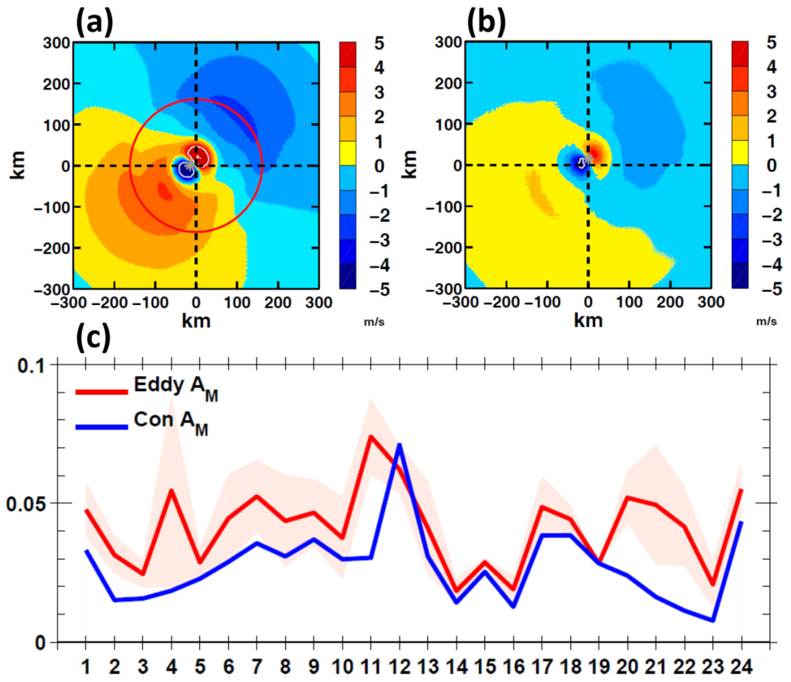
3.2.1. Warm-Eddy-Induced Amplified Circulation

We begin by describing the warm-eddy induced primary (swirling) and secondary (overturning) circulation response. We azimuthally average each experiment’s atmospheric variables around the typhoon centre, defined as the minimum SLP. Then, we take the variables’ differences for each ensemble member pair (eddy minus control), ensemble-average them, and plot them in the radial and vertical section view. Figure 4 shows the results for members in the upper-quartile of intensity on day 5 when the response is near the maximum. The warm eddy induces (i) an increased vertical velocity along the eyewall (Figure 4a vectors and red shading), (ii) an increased outflow in the upper troposphere at ~200 hPa (Figure 4a vectors, and Figure 4c red shading), (iii) a decreased core pressure (Figure 4a, blue dashed contours), and (iv) an intensified azimuthal wind with a maximum just inside the eyewall near the edge of the boundary layer at z ≈ 1 km height (Figure 4b red shading and solid contours), coinciding with where (v) there is a radial convergence into the eyewall in the boundary layer (Figure 4c blue shading and dashed contours).
We now identify processes responsible for the increased intensity response due to the warm eddy. We tested various parameters that can affect intensity change [52]. We found that low-level moisture flux convergence (MFC) and intensity are most closely related. To show this, we calculate MFC from 1000 hPa to 700 ha [21]:
M F C = 1 ρ g 1000 700 · ( u q ) d p .
Here, q is the specific humidity, p is pressure, ρ is density, and g is gravity. We then average ΔMFC and ΔV from days 3 to 7 and regress them (Figure 5). The plot indicates a significant correlation between ΔV and ΔMFC, consistent with previous theoretical and observational analyses [16,21,64]. Thus, the warm eddy increases the upward transfer of surface enthalpy flux and moisture convergence in the cyclone core, accompanied by stronger updrafts and increased azimuthal wind speeds.

3.2.2. Probability Density Function of Lifetime Maximum Intensity

The large sample of modelled typhoons enables us to calculate the number of storms grouped by their lifetime maximum intensity (LMI), expressed as the probability density function PDF.
Figure 6a compares the PDF for the control (blue bars) and the warm eddy (red bars) experiments. The control experiment PDF shows a bimodal distribution with two peaks: a primary peak in the 35–40 m/s (“minor-category”) intensity range and a secondary peak in the 55–60 m/s (“major-category”) intensity range. The warm eddy experiment PDF also shows a bimodal distribution. The primary peak is less conspicuous and is shifted to the right, confirming that warm eddy can make a passing storm more intense. However, for stronger storms with LMI > 45 m/s, the PDF is similar to the control PDF (except the 50–55 m/s range where Eddy PDF shows a small value). To understand these behaviours, we separate the storms into a subgroup that undergo RI at least once in their lifetime and the remaining subgroup of storms that do not have any RI. We calculate their PDF and denote them as PDFRI and PDFnonRI.
Figure 6b plots the PDFRI (solid lines) and PDFnonRI (dashed lines) for the control (blue colour) and warm eddy (red colour) experiments. The 35–40 m/s intensity range is entirely (100%) made up of non-RI storms for the control experiments. Therefore, the non-RI storms wholly contribute to the primary peak of the control experiment in Figure 6a. On the other hand, the 55–60 m/s intensity range is dominated by RI storms (67%), while the remaining 33% is due to the non-RI storms. Therefore, the secondary peak seen in the control PDF of Figure 6a is primarily due to the RI storms. In other words, storms that undergo rapid intensification tend to evolve into “major-category” storms. The bimodal distribution and its connection with RI and non-RI storms are very similar to the characteristics found for observed tropical cyclones [2,3].
The warm eddy experiments behave in much the same way. Figure 6b shows that the rightward shift of the primary peak in PDF is due entirely (100%) to non-RI storms. The RI storms again account for most (67%) of the secondary peak. They tend to evolve into “major-category” storms as in the control experiments. However, the warm eddy PDFRI is nearly identical to the control PDFRI, which means that the intensification due to warm eddy is insufficient to yield more RI events. The PDF results of the large ensemble experiments do not pass Step 2 of the WOF-RI hypothesis test.

3.2.3. Vortex Asymmetry

Although the warm eddy experiments produce some storm intensification, they do not yield more RI events than the control experiments. Are there aspects of the warm eddy experiments that can tame the intensification rate and prevent the modelled storm from triggering additional RI events?
Previous studies have shown that vortex asymmetry is not favourable to intensification [16,19,65]. The model develops asymmetry with or without the warm eddy (see, for example, Figure 2; also [39]). However, finite translation and wind-dependent surface enthalpy fluxes introduce asymmetric perturbations to the cyclone. We examined if across the ensemble warm eddy experiments’ vortices are significantly more asymmetrical than the otherwise identical control experiments without the warm eddy. We define asymmetry (A) as the deviation of the speed of 1000–200 hPa depth-averaged wind ( U ¯ ) from the azimuthally averaged (denoted by <.>) wind of the Control experiment:
A ( r , θ , t ) = | U ¯ | | < U ¯ c o n > | ,   U ¯ = 1000 h P a 200 h P a u d p / 800 h P a .
Here, u(r,θ,p,t) is the wind at the radial (r), azimuthal (θ), pressure level (p), and time (t). The subscript “con” denotes ‘control.’ (We tested other ways to define asymmetry, for example, using the 10-m wind or the Zhang and Oey’s [21] moisture flux convergence. All give very similar results. The form adopted here gives, in the limit of the Control solution being symmetrical: U ¯ c o n   < U ¯ c o n > , we have Acon → 0; also, Aeddy → 0 in the additional limit of a vanishing eddy).
Figure 7a,b show an example of Aeddy (a) compared with the corresponding Acon (b). Both show a mixed radial mode-1 plus azimuthal mode-1 pattern [66]. The Aeddy pattern is rotated roughly 7° anticlockwise relative to the Acon pattern. However, this relative rotation does not affect asymmetry as we can eliminate it by adjusting the azimuthal origin. Figure 7a,b shows that the magnitude of Aeddy is larger than Acon, and it is clear that for this example, the Aeddy is more asymmetric than Acon.
To quantitatively compare all Eddy and Control asymmetries, we define an asymmetry metric (AM). We first collocate all storms to a common centre (x, y) = (0, 0) defined, as before, as where the SLP is minimum. We then sort storms for which the Aeddy has a greater or equal number of zero crossings than the corresponding Acon along the principal direction within a radial distance of 200 km. Beyond this distance, the A-values are very small. In the examples shown in Figure 7a,b, the principal directions are 45° and 38° for Aeddy and Acon, respectively, and each has three zero-crossings. The majority (97%) of Aeddy and Acon satisfy this condition. The remaining members (3%) not satisfying the condition have very weak amplitudes, and we discarded them. (They have no visible effects on the result if included). Finally, we area-average the absolute value of A and normalise it by the maximum speed (S) of the 1000–200 hPa depth-averaged wind:
A M ( t ) = | A | d r d θ / ( S d r d θ ) ,   S ( t ) = M a x ( | U ¯ | ) .
Here, the double integral is over a circle of 200 km centred at (x, y) = (0, 0). According to (3), larger AM indicates greater asymmetry. Note that the Eddy experiment’s S is almost always larger than the Control experiment’s S. The normalising tends to decrease the Eddy AM.
Figure 7c shows the Eddy and Control AM’s for the ensemble experiments, organised according to 24 groups of the Control experiment (see caption). All but one (group#12) have larger AM for the eddy than the Control experiments. The “total mean ± s.d.” for all 24 groups for Eddy and Control experiments are statistically significantly different: (4.2 ± 0.37) × 10−2 and (2.75 ± 0.53) × 10−2. These results indicate a more significant asymmetry of the simulated vortex in the Eddy experiments than the Control experiments. We conclude that, while the presence of warm eddy can intensify the storm, the warm eddy-induced perturbation also produces a greater asymmetry in the vortex. That tends to tame intensification and prevent the modelled storm from intensifying rapidly.

4. Discussion

Several studies have observed anecdotes of an apparent connection between warm eddies and RI events. We discuss three cases here. Shay et al. [4] noted that Hurricane Opal (1995) rapidly intensified as it passed over a Loop Current warm eddy. Lin et al. [5] associated Typhoon Maemi’s (2003) RI with the storm crossing a warm eddy in the Philippine Sea. Oey and Lin [23] noted that Typhoon Soudelor (2015) underwent multiple RIs while crossing a series of warm eddies in the Philippine Sea.
However, unlike the idealised model used in the present study, isolating the warm eddy’s influence on intensity change from observations or realistic model simulations poses a challenge. In addition to the storm’s internal dynamics, typhoon intensity change depends on other environmental factors besides warm eddies. Perhaps the environmental vertical wind shear (Vs) is the most documented. Strong wind shear vs. ≳10 m/s is detrimental to intensification [26]. Wind shear vs. <10 m/s favours intensification and vs. ≲4 m/s favours rapid intensification [67]. Bozart et al. [68] found that Hurricane Opal’s rapid intensification also coincided with when the environmental vertical wind shear became very weak, vs. <4 m/s, an environment that is favourable for RI [67]. Oey and Lin [23] showed that Typhoon Maemi’s RI coincided with the storm entering and exiting a pocket (closed contour) of low vs. <4 m/s. Oey and Lin [23] conducted an environmental attribution analysis of Typhoon Soudelor. They concluded that the contribution to the storm’s intensity variation due to vs. is the largest (62%), followed by warm eddies’ Z26 (27%) and others. The multiple RIs coincided with the storm entering a pocket of low vs. <4 m/s in the Philippine Sea.
Kowch and Emanuel [59] analyzed multiyear global data and concluded that random environmental and internal variability primarily control RI. Zhang and Oey [21] found no statistically significant preference that RI develops over warm eddies in the global ocean. Thus, attributing observed RI events to warm eddies alone is potentially incomplete. Our finding that there is no statistically significantly different number of RI in eddy and non-eddy experiments is not inconsistent with these observations. On the other hand, in agreement with the model, observations indicate that warm eddies can intensify a passing storm, and intensity forecasts incorporating warm eddies are improved [24,25].
This study shows that a typhoon passing a warm eddy develops a greater vortex asymmetry than without the eddy. The asymmetry works against the intensity-boosting effect of the warm eddy. It lessens the chance for RI and decreases RI events that may otherwise develop in the eddy experiments.
On the other hand, the reason why a warm eddy cannot easily trigger RI may be more fundamental. As a storm passes over a warm eddy, the increased SST δTe due to the eddy increases its maximum potential intensity (MPI) [13], δVm. This δVm represents an upper-bound increased wind due to the eddy. Figure 8 shows δVm (colour shading) as a function of δTe and the ambient SST To. The δVm = 15.4 m/s black line separates the upper-right (δTe, To)-space where a warm-eddy induced RI is possible from the lower-left space where RI is impossible. For To ≲ 29 °C and δTe ≲ 1 °C presently observed in the western North Pacific, warm eddy-induced RI events are unlikely.
With ocean feedback, an increased δVm increases upper-ocean mixing, producing SST cooling. The cooling would reduce δVm, which in turn modifies the amount of cooling in a coupled manner. Our WRF-POM experiments include these and other complex processes. In the Appendix A, we derive an analytical solution to include only the essential features of the coupled process. To the first order, the solution is (Appendix A Equation (A5)):
δVm = a × δTe/(1 + b × FT).
Here, a and b are ambient state-dependent coefficients. The a × δTe is the MPI estimate of the warm eddy-induced intensification. The b × FT (>0) is the coupling term that includes the contribution (FT) from ocean cooling caused by the translating storm. The formula shows that ocean cooling always reduces δVm. The FT is inversely proportional to Uh and the square of the upper-ocean thickness (e.g., Z26): FT ~ 1/(Uh Z262). Thus, the ocean cools more for slower storms or thinner Z26, or both, which reduces δVm. For very deep Z26 ~ ∞, FT vanishes, and ocean feedback is negligible. Ocean feedback is also weak for very fast storms since there is then little time for ocean mixing and the feedback to the storm is negligible. Intensification is then due to the warm eddy alone and becomes the MPI estimate: δVm = a × δTe. In Figure 8, we plot the δVm = 15.4 m/s lines (dashed blue) obtained from the coupled solution and display them for different Uh. Ocean cooling shifts the (δTe, To)-space for RI further to the upper right, making it harder for warm eddy-induced RI to develop. For RI to develop, the eddy and ambient climatology would have to be exceedingly warmer than their present-day values of δTe ≲ 1 °C and To ≲ 29 °C.

5. Conclusions

This study examines if an ocean’s warm eddy may cause a passing typhoon to undergo rapid intensification. We conducted a large ensemble of numerical experiments covering a wide range of model parameters and observed quantities applicable to the western North Pacific typhoon region. The model excludes the environmental vertical wind shear and storm translation and focuses only on the warm eddy’s influence. We use twin experiments with and without the warm eddy to calculate the warm eddy’s influence. The results show that the warm eddy’s presence increases the low-level moisture convergence flux into the passing typhoon’s core, intensifying the storm. However, the warm eddy also increases the storm’s asymmetry, which tends to tame intensity. As a result, the experiments with warm eddy do not show a statistically significantly different number of rapid intensification events than the experiments without the eddy. A simple analytical model supports the numerical model’s conclusion. It provides an upper-bound estimate of warm eddy-induced intensification and shows, in particular, how ocean feedback always reduces the chance for RI.
Our results are applicable to storms translating at supercritical speeds Uh > 3 m/s, for which 1D ocean mixing is approximately valid. Future work should extend using a full 3D ocean model to examine RI in slow storms over warm water.

Author Contributions

L.O. conducted the analyses and wrote the paper. S.H. conducted model simulations and analyses, and prepared the graphics. Both authors have read and agreed to the published version of the manuscript.

Funding

This research was funded by the Ministry of Science and Technology of Taiwan, grant numbers 107-2111-M-008-035 and 107-2611-M-008-003.

Institutional Review Board Statement

Not applicable.

Informed Consent Statement

Not applicable.

Data Availability Statement

The observational data presented in this study are available from the cited references. Model data are available from the authors upon request. The analytical model’s complete derivation is in a Lecture Note available from the senior author L.O.

Conflicts of Interest

The authors declare no conflict of interest. The funders had no role in the design of the study; in the collection, analyses, or interpretation of data; in the writing of the manuscript, or in the decision to publish the results.

Appendix A. An Analytical, Air-Sea Coupled Model of WOF-Induced Intensification

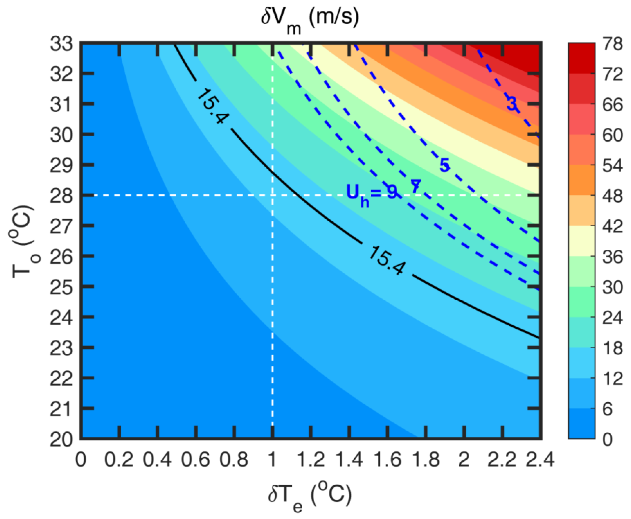
Appendix A.1. Increased Intensity Due to WOF

A typhoon encounters a WOF (e.g., a warm eddy) with surface temperature δTe warmer than the ambient SST To The warmer SST increases the wind, which we can estimate using the maximum potential intensity theory [13]. We use the empirical form given by DeMaria and Kaplan [69]:
Vm = A + B eC(T − 30),
where Vm (m/s) is the maximum wind, T (°C) is the SST, and A = 15.69 m/s, B = 98.03 m/s, and C = 0.1806 °C−1 are for the western North Pacific [17]. Thus
δVm = (∂Vm/∂T)|o δT + (∂2Vm/∂T2)|o δT2/2 + O(δT3);
where (..)|o means evaluation at the ambient state To. Setting δT = δTe gives an estimate of the increased intensity as the storm encounters the warm eddy. Figure 8 plots δVm (colour shading) as a function of δTe and To. The δVm = 15.4 m/s solid line delineates the (δTe, To)-space on the upper right (lower left) where a warm-eddy induced RI is possible (impossible).

Appendix A.2. Ocean Cooling

The increased δVm due to the warm eddy increases upper-ocean mixing, producing SST cooling. The cooling would reduce δVm, which then modifies the amount of cooling in a coupled manner. We now formulate a simple ocean model to achieve the coupling.
We assume no horizontal variation and divide the near-surface ocean into two active layers of thicknesses h1 and h2. Layer 1 consists of warm water of uniform temperature T1 from sea-surface to z = −h1. Layer 2 consists of cooler water of uniform temperature T2 (<T1) from z = −h1 to z = −h2. There is also a third, deep layer from z = −h2 to the ocean bottom, which we assume to be inactive and needs not concern us. We first obtain the SST cooling due to a travelling storm by equating the potential energy required for the two layers to mix into a single layer of uniform temperature to (a fraction of) the wind energy of the storm. We then obtain the change in SST due to change in the maximum wind as (after some algebra):
δTO = −FT δVo + O(δVo2),
FT = (L/Uh)(ρao)[4/(3π)][h2/(h1 + h2)][(γCd)3Vo2]/[(g/2)αh2h1].
Here,
δTO = Tmix − T1 is the change in SST due to δVm;
Tmix = the uniform temperature of the mixed, single layer;
δVo is the change in the maximum wind;
Vo is the maximum wind of the incoming storm, taken to be 30 m/s;
L is the storm’s radius, ≈ 200 km from core to ~18 m/s [70];
Uh is the storm’s translation speed;
ρao is the ratio of air to seawater densities, ≈ 10−3;
γ is the “mixing efficiency”, ≈ 0.02 [71];
Cd is the wind drag coefficient, ≈ 2 × 10⁻³ [46];
g is the earth’s gravity, ≈ 10 m/s2;
α is seawater’s thermal expansion coefficient, ≈ 3 × 10⁻⁴ K−1 [72];
h1 is Layer 1′s depth, ≈ 100 m; and
h2 is Layer 2′s depth, ≈ 100 m.
At the location where we calculate δTO, the SST is mixed and cooled by (a fraction of) the time-integrated wind power of the storm as it approaches and arrives in time ≈ (L/Uh). This SST cooling is the “ahead-of-storm” cooling caused by the front half of the storm [56]. The “back half” cooling occurs after the storm’s core has left and is assumed to have negligible effects on the storm’s intensity.
The factor “4/(3π)” accounts for wind energy input into the ocean, caused by a wind that rises to the maximum Vo as the storm’s front half arrives; then the wind drops to zero, modelled as Wind = Vo sin[πtUh/(2L)], for 0 ≤ t ≤ L/Uh, = 0 otherwise.
The mixing efficiency γ takes into account that only a fraction of the wind power goes into mixing. The value of γ = 0.02 is for strong boundary stirring at high buoyancy Reynolds number [71,73,74,75], which we assume is the case of upper-ocean mixing by a tropical cyclone.
The values of h1 ≈ 100 m and h2 ≈ 100 m are typically observed in the RI region in western North Pacific for the depths from surface to the 26 °C isotherm z = −Z26, and from z = −Z26 to the 20 °C isotherm z = −Z20 [32].

Appendix A.3. The Coupling

To close the model and incorporate air-sea coupling, we set δVo = δVm in (A3) and substitute
δT = δTe + δTO
into (A2) to obtain the desired equation for δVm (Setting δVo = δVm to close the model would likely overestimate the effect of ocean cooling, since δVo is generally less than δVm. However, the upper-bound δVm in (A5; or the full quadratic form) and the qualitative effect of ocean cooling are unchanged). Keeping only the linear δT term, the equation is:
δVm = [(∂Vm/∂T)|o δTe]/[1 + (∂Vm/∂T)|o FT].
It shows that ocean cooling decreases the intensification which the storm would otherwise achieve with warm eddy alone without the cooling. Note that FT is inversely proportional to Uh, the upper-layer depth h1, and the total depth (h1 + h2):
FT ~ 1/[Uh h1 (h1 + h2)].
Therefore, the decreased intensification by ocean cooling is more for slow storms. On the other hand, the effect of SST cooling diminishes with a thicker upper layer, like (h1)−2. The δVm increases to its warm eddy-induced intensification (i.e., due to δTe alone) for very fast storms or when the warm upper layer is very thick. For very fast storm, there is little time for ocean cooling and feedback to the storm. For very thick upper layer, it is harder to entrain cool lower-layer water to the surface.
Figure 8 shows the δVm = 15.4 m/s (blue dashed lines) obtained from (A2), (A3) and (A4) for various Uh. The 15.4 black line is for Uh = ∞. Ocean cooling shifts the 15.4 m/s line further to the upper right, making it harder for a warm eddy-induced RI to develop.

References

  1. Kaplan, J.; DeMaria, M. Large-scale characteristics of rapidly intensifying tropical cyclones in the North Atlantic basin. Weather Forecast. 2003, 18, 1093–1108. [Google Scholar] [CrossRef] [Green Version]
  2. Kossin, J.P.; Olander, T.L.; Knapp, K.R. Trend analysis with a new global record of tropical cyclone intensity. J. Clim. 2013, 26, 9960–9976. [Google Scholar] [CrossRef]
  3. Lee, C.-Y.; Tippett, M.K.; Sobel, A.H.; Camargo, S.J. Rapid intensification and the bimodal distribution of tropical cyclone intensity. Nat. Commun. 2016, 7, 10625. [Google Scholar] [CrossRef] [PubMed]
  4. Shay, L.K.; Goni, G.J.; Black, P.G. Effects of a warm oceanic feature on Hurricane Opal. Mon. Weather Rev. 2000, 128, 1366–1383. [Google Scholar] [CrossRef]
  5. Lin, I.I.; Wu, C.C.; Emanuel, K.; Lee, I.H.; Wu, C.R.; Pun, I.F. The interaction of Supertyphoon Maemi (2003) with a warm ocean eddy. Mon. Weather Rev. 2005, 2635–2649. [Google Scholar] [CrossRef]
  6. Ali, M.M.; Jagadeesh, P.V.; Jain, S. Effects of eddies on Bay of Bengal cyclone intensity. Eos Trans. Am. Geophys. Union 2007, 88, 93–95. [Google Scholar] [CrossRef]
  7. Mawren, D.; Reason, C.J.C. Variability of upper-ocean characteristics and tropical cyclones in the South West Indian Ocean. J. Geophys. Res. Oceans 2017, 122, 2012–2028. [Google Scholar] [CrossRef]
  8. Potter, H.; DiMarco, S.F.; Knap, A.H. Tropical Cyclone Heat Potential and the Rapid Intensification of Hurricane Harvey in the Texas Bight. J. Geophys. Res. Oceans 2019, 124, 2440–2451. [Google Scholar] [CrossRef]
  9. Gray, W.M. The formation of tropical cyclones. Meteor. Atmos. Phys. 1998, 67, 37–69. [Google Scholar] [CrossRef]
  10. Chang, Y.L.; Oey, L.Y. Interannual and seasonal variations of Kuroshio transport east of Taiwan inferred from 29 years of tide-gauge data. Geophys. Res. Lett. 2011, 38, L08603. [Google Scholar] [CrossRef]
  11. Chelton, D.B.; Schlax, M.G.; Samelson, R.M. Global observations of nonlinear mesoscale eddies. Prog. Oceanogr. 2011, 91, 167–216. [Google Scholar] [CrossRef]
  12. Sun, J.; Xu, F.H.; Oey, L.Y.; Lin, Y.L. Monthly variability of Luzon Strait tropical cyclone intensification over the Northern South China Sea in recent decades. Clim. Dyn. 2019, 52, 3631–3642. [Google Scholar] [CrossRef]
  13. Emanuel, K.A. An air-sea interaction theory for tropical cyclones. Part I: Steady-state maintenance. J. Atmos. Sci. 1986, 43, 585–605. [Google Scholar] [CrossRef]
  14. Merrill, R.T. Environmental influences on hurricane intensification. J. Atmos. Sci. 1988, 45, 1678–1687. [Google Scholar] [CrossRef] [Green Version]
  15. DeMaria, M.; Kaplan, J.; Baik, J.J. Upper-level eddy angular momentum fluxes and tropical cyclone intensity change. J. Atmos. Sci. 1993, 50, 1133–1147. [Google Scholar] [CrossRef] [Green Version]
  16. Peng, M.S.; Jeng, B.; Williams, R.T. A numerical study on tropical cyclone intensification. Part I: Beta effect and mean flow effect. J. Atmos. Sci. 1999, 56, 1404–1423. [Google Scholar] [CrossRef]
  17. Zeng, Z.; Wang, Y.; Wu, C.C. Environmental dynamical control of tropical cyclone intensity—An observational study. Mon. Weather Rev. 2007, 135, 38–59. [Google Scholar] [CrossRef] [Green Version]
  18. Hendricks, E.A.; Peng, M.S.; Fu, B.; Li, T. Quantifying environmental control on tropical cyclone intensity change. Mon. Weather Rev. 2010, 138, 3243–3271. [Google Scholar] [CrossRef] [Green Version]
  19. Kaplan, J.; DeMaria, M.; Knaff, J.A. A revised tropical cyclone rapid intensification index for the Atlantic and eastern North Pacific basins. Weather Forecast. 2010, 25, 220–241. [Google Scholar] [CrossRef]
  20. Wu, L.; Su, H.; Fovell, R.G.; Wang, B.; Shen, J.T.; Kahn, B.H.; Hristova-Veleva, S.M.; Lambrigtsen, B.H.; Fetzer, E.J.; Jiang, J.H. Relationship of environmental relative humidity with North Atlantic tropical cyclone intensity and intensification rate. Geophys. Res. Lett. 2012, 39, L20809. [Google Scholar] [CrossRef] [Green Version]
  21. Zhang, L.; Oey, L. Young ocean waves favor the rapid intensification of tropical cyclones—A global observational analysis. Mon. Weather Rev. 2019, 147, 311–328. [Google Scholar] [CrossRef]
  22. Rogers, R.; Aberson, S.; Black, M.; Black, P.; Cione, J.; Dodge, P.; Surgi, N. The intensity forecasting experiment: A NOAA multiyear field program for improving tropical cyclone intensity forecasts. Bull. Am. Meteorol. Soc. 2006, 87, 1523–1537. [Google Scholar] [CrossRef] [Green Version]
  23. Oey, L.; Lin, Y. The Influence of Environments on the Intensity Change of Typhoon Soudelor. Atmosphere 2021, 12, 162. [Google Scholar] [CrossRef]
  24. Mainelli, M.; DeMaria, M.; Shay, L.K.; Goni, G. Application of oceanic heat content estimation to operational forecasting of recent Atlantic category 5 hurricanes. Weather Forecast. 2008, 23, 3–16. [Google Scholar] [CrossRef]
  25. Balaguru, K.; Foltz, G.R.; Leung, L.R.; Hagos, S.M.; Judi, D.R. On the use of ocean dynamic temperature for hurricane intensity forecasting. Weather Forecast. 2018, 33, 411–418. [Google Scholar] [CrossRef]
  26. Frank, W.M.; Ritchie, E.A. Effects of vertical wind shear on the intensity and structure of numerically simulated hurricanes. Mon. Weather Rev. 2001, 129, 2249–2269. [Google Scholar] [CrossRef]
  27. Wu, L.G.; Braun, S.A. Effects of environmentally induced asymmetries on hurricane intensity: A numerical study. J. Atmos. Sci. 2004, 61, 3065–3081. [Google Scholar] [CrossRef]
  28. Fiorino, M.; Elsberry, R.L. Some aspects of vortex structure related to tropical cyclone motion. J. Atmos. Sci. 1989, 46, 975–990. [Google Scholar] [CrossRef] [Green Version]
  29. Oey, L.-Y. The formation and maintenance of density fronts on US southeastern continental shelf during winter. J. Phys. Oceanogr. 1986, 16, 1121–1135. [Google Scholar] [CrossRef] [Green Version]
  30. Chiang, T.L.; Wu, C.R.; Oey, L.Y. Typhoon Kai-Tak: A perfect ocean’s storm. J. Phys. Oceanogr. 2011, 41, 221–233. [Google Scholar] [CrossRef]
  31. Huang, S.M.; Oey, L.Y. Right-side cooling and phytoplankton bloom in the wake of a tropical cyclone. J. Geophys. Res. Oceans 2015, 120, 5735–5748. [Google Scholar] [CrossRef]
  32. Sun, J.; Oey, L.Y.; Chang, R.; Xu, F.; Huang, S.M. Ocean response to typhoon Nuri (2008) in western Pacific and South China Sea. Ocean Dyn. 2015, 65, 735–749. [Google Scholar] [CrossRef]
  33. Emanuel, K.A. Thermodynamic control of hurricane intensity. Nature 1999, 401, 665–669. [Google Scholar] [CrossRef]
  34. Michalakes, J.; Chen, S.-H.; Dudhia, J.; Hart, L.; Klemp, J.; Middlecoff, J.; Skamarock, W. Development of a next-generation regional weather research and forecast model. In Developments in Teracomputing, Proceedings of the Ninth ECMWF Workshop on the Use of High Performance Computing in Meteorology, Reading, UK, 13–17 Novmber 2000; Kreitz, N., Zwieflhofer, W., Eds.; World Scientific: London, UK, 2001; pp. 269–276. [Google Scholar]
  35. Mellor, G.L. Users Guide for a Three-Dimensional, Primitive Equation, Numerical Ocean Model; Princeton University: Princeton, NJ, USA, 2004; p. 56. Available online: http://jes.apl.washington.edu/modsims_two/usersguide0604.pdf (accessed on 18 June 2021).
  36. Oey, L.-Y.; Mellor, G.L.; Hires, R.I. A three-dimensional simulation of the Hudson-Raritan estuary. Part I: Description of the model and model simulations. J. Phys. Oceanogr. 1985, 15, 1676–1692. [Google Scholar] [CrossRef] [Green Version]
  37. Oey, L.; Chang, Y.; Lin, Y.-C.; Chang, M.-C.; Xu, F.-H.; Lu, H.-F. ATOP—The Advanced Taiwan Ocean Prediction System based on the mpiPOM. Part 1: Model descriptions, analyses and results. Terr. Atmos. Ocean. Sci. 2013, 24, 137–158. [Google Scholar] [CrossRef] [Green Version]
  38. Rotunno, R.; Emanuel, K.A. An Air–Sea Interaction Theory for Tropical Cyclones. Part II: Evolutionary Study Using a Nonhydrostatic Axisymmetric Numerical Model. J. Atmos. Sci. 1987, 44, 542–561. [Google Scholar] [CrossRef] [Green Version]
  39. Montgomery, M.T.; Persing, J.; Smith, R.K. Putting to rest WISHE-ful misconceptions for tropical cyclone intensification. J. Adv. Model. Earth Syst. 2015, 7, 92–109. [Google Scholar] [CrossRef] [Green Version]
  40. Murthy, V.S.; Boos, W.R. Role of surface enthalpy fluxes in idealized simulations of tropical depression spinup. J. Atmos. Sci. 2018, 75, 1811–1831. [Google Scholar] [CrossRef]
  41. Hong, S.Y.; Noh, Y.; Dudhia, J. A new vertical diffusion package with an explicit treatment of entrainment processes. Mon. Weather Rev. 2006, 134, 2318–2341. [Google Scholar] [CrossRef] [Green Version]
  42. Kessler, E. On the Distribution and Continuity of Water Substance in Atmospheric Circulation. Meteor. Monogr. Am. Meteor. Soc. 1969, 32, 84. [Google Scholar]
  43. Hong, S.Y.; Lim, J.O.J. The WRF single-moment 6-class microphysics scheme (WSM6). Asia Pac. J. Atmos. Sci. 2006, 42, 129–151. [Google Scholar]
  44. Mansell, E.R.; Ziegler, C.L.; Bruning, E.C. Simulated electrification of a small thunderstorm with two–moment bulk microphysics. J. Atmos. Sci. 2010, 67, 171–194. [Google Scholar] [CrossRef]
  45. Stensrud, D.J. Parameterization Schemes. Keys to Understanding Numerical Weather Prediction Models; Cambridge University Press: Cambridge, UK, 2007; p. 579. [Google Scholar]
  46. Powell, M.D.; Vickery, P.J.; Reinhold, T.A. Reduced drag coefficient for high wind speeds in tropical cyclones. Nature 2003, 422, 279–283. [Google Scholar] [CrossRef]
  47. Donelan, M.; Haus, B.; Reul, N.; Plant, W.; Stiassnie, M.; Graber, H.; Brown, O.; Saltzman, E. On the limiting aerodynamic roughness of the ocean in very strong winds. Geophys. Res. Lett. 2004, 31, L18306. [Google Scholar] [CrossRef] [Green Version]
  48. Davis, C.; Wang, W.; Chen, S.S.; Chen, Y.; Kristen, C.; Mark, D.M.; Jimy, D.; Greg, H.; Joe, K.; John, M. Prediction of landfalling hurricanes with the advanced hurricane WRF model. Mon. Weather Rev. 2008, 136, 1990–2005. [Google Scholar] [CrossRef] [Green Version]
  49. Mellor, G.L.; Yamada, T. Development of a turbulence closure model for geophysical fluid problems. Rev. Geophys. Space Phys. 1982, 20, 851–875. [Google Scholar] [CrossRef] [Green Version]
  50. Holliday, C.R.; Thompson, A.H. Climatological characteristics of rapidly intensifying typhoons. Mon. Weather Rev. 1979, 107, 1022–1034. [Google Scholar] [CrossRef]
  51. Wada, A. Unusually rapid intensification of Typhoon Man-yi in 2013 under preexisting warm-water conditions near the Kuroshio front south of Japan. J. Oceanogr. 2015, 131–156. [Google Scholar] [CrossRef]
  52. Sun, J.; Oey, L.; Xu, F.; Lin, Y.C. Sea level rise, surface warming, and the weakened buffering ability of South China Sea to strong typhoons in recent decades. Nature Sci. Rep. 2017, 7, 7418. [Google Scholar] [CrossRef] [PubMed]
  53. Zhang, L.; Oey, L. An observational analysis of ocean surface waves in tropical cyclones in the western North Pacific Ocean. J. Geophys. Res. Oceans 2019, 124, 184–195. [Google Scholar] [CrossRef]
  54. Lin, Y.-C.; Oey, L.Y. Rainfall-enhanced blooming in typhoon wakes. Nature Sci. Rep. 2016, 6, 31310. [Google Scholar] [CrossRef] [PubMed] [Green Version]
  55. Price, J.F. Upper Ocean Response to a Hurricane. J. Phys. Oceanogr. 1981, 11, 153–175. [Google Scholar] [CrossRef] [Green Version]
  56. Oey, L.Y.; Ezer, T.; Wang, D.P.; Fan, S.J.; Yin, X.Q. Loop current warming by Hurricane Wilma. Geophys. Res. Lett. 2006, 33, L08613. [Google Scholar] [CrossRef] [Green Version]
  57. Oey, L.Y.; Ezer, T.; Wang, D.P.; Yin, X.Q.; Fan, S.J. Hurricane-induced motions and interaction with ocean currents. Cont. Shelf Res. 2007, 27, 1249–1263. [Google Scholar] [CrossRef]
  58. Xu, F.H.; Oey, L.Y. Seasonal SSH variability of the Northern South China Sea. J. Phys. Oceanogr. 2015, 45, 1595–1609. [Google Scholar] [CrossRef]
  59. Kowch, R.; Emanuel, K. Are special processes at work in the rapid intensification of tropical cyclones? Mon. Weather Rev. 2015, 143, 878–882. [Google Scholar] [CrossRef] [Green Version]
  60. Hong, X.; Chang, S.W.; Raman, S.; Shay, L.K.; Hodur, R. The interaction between Hurricane Opal (1995) and a warm core ring in the Gulf of Mexico. Mon. Weather Rev. 2000, 128, 1347–1365. [Google Scholar] [CrossRef] [Green Version]
  61. Wang, Z.; Zhang, G.; Peng, M.S.; Chen, J.H.; Lin, S.J. Predictability of Atlantic tropical cyclones in the GFDL HiRAM model. Geophys. Res. Lett. 2015, 42, 2547–2554. [Google Scholar] [CrossRef]
  62. Huang, S.-M.; Oey, L.Y. Malay Archipelago forest loss to cash crops and urban contributes to weaken the Asian summer monsoon: An atmospheric modeling study. J. Clim. 2019, 32, 3189–3205. [Google Scholar] [CrossRef]
  63. Lin, Y.-C.; Oey, L.Y. Global trends of sea surface gravity wave, wind and coastal wave set-up. J. Clim. 2020, 32, 769–785. [Google Scholar] [CrossRef]
  64. Riehl, H. Some relations between wind and thermal structure of steady state hurricanes. J. Atmos. Sci. 1963, 20, 276–287. [Google Scholar] [CrossRef] [Green Version]
  65. Nolan, D.S.; Grasso, L.D. Three-dimensional perturbations to balanced, hurricane-like vortices. Part II: Symmetric response and nonlinear simulations. J. Atmos. Sci. 2003, 60, 2717–2745. [Google Scholar] [CrossRef] [Green Version]
  66. McCalpin, J.D. On the adjustment of azimuthally perturbed vortices. J. Geophys. Res. 1987, 92, 8213–8225. [Google Scholar] [CrossRef]
  67. Paterson, L.A.; Hanstrum, B.N.; Davidson, N.E.; Weber, H.C. Influence of Environmental Vertical Wind Shear on the Intensity of Hurricane-Strength Tropical Cyclones in the Australian Region. Mon. Weather Rev. 2005, 133, 3644–3660. [Google Scholar] [CrossRef]
  68. Bozart, L.E.; Velden, C.S.; Bracken, W.D.; Molinari, J.; Black, P.G. Environmental influences on the rapid intensification of Hurricane Opal (1995) over the Gulf of Mexico. Mon. Weather Rev. 2000, 128, 322–352. [Google Scholar] [CrossRef]
  69. DeMaria, M.; Kaplan, J. Sea surface temperature and the maximum intensity of Atlantic tropical cyclones. J. Clim. 1994, 7, 1325–1334. [Google Scholar] [CrossRef] [Green Version]
  70. Holland, G.J.; Belanger, J.I.; Fritz, A. A revised model for radial profiles of hurricane winds. Mon. Weather Rev. 2010, 138, 4393–4401. [Google Scholar] [CrossRef]
  71. Monismith, S.G.; Koseff, J.R.; White, B.L. Mixing efficiency in the presence of stratification: When is it constant? Geophys. Res. Lett. 2018, 45, 5627–5634. [Google Scholar] [CrossRef]
  72. Gill, A.E. Atmosphere-Ocean. Dynamics; Academic Press: Cambridge, MA, USA, 1982; p. 662. [Google Scholar]
  73. Etemad-Shahidi, A.; Imberger, J. Anatomy of turbulence in a narrow and strongly stratified estuary. J. Geophys. Res. 2002, 107, 3070. [Google Scholar] [CrossRef]
  74. Bouffard, D.; Boegman, L. A Diapycnal diffusivity model for stratified environmental flows. Dyn. Atmos. Oceans 2013, 61, 14–34. [Google Scholar] [CrossRef]
  75. Smyth, W.D. Marginal instability and the efficiency of ocean mixing. J. Phys. Oceanogr. 2020, 50, 2141–2150. [Google Scholar] [CrossRef]
Figure 1. (Top) plan-view plots of 10-m wind (vectors; for clarity, vector length is the same for speeds >50 m/s, and vectors with speeds <25 m/s are not plotted) superimposed on SST (shading) at days 2, 3, and 4; and (Bottom) vertical xz-section plots of ocean temperature (shading with black contours 18, 20, 28 °C, gray contours 27.5 and 27.9 °C and magenta contours 28.1 and 28.5 °C.
Atmosphere 12 00797 g001
Figure 2. Vertical vorticity ζ × 104 (s−1) at z=1 km on days 2, 3, 4, and 5 (from top to bottom rows) for (left) the control and (right) the warm-eddy experiment. Blue contours: ζ = (−3, −1) × 10−4 s−1, black: ζ = (3, 6) × 10−4 s−1, red: ζ = 20 × 10−4 s−1, white: ζ = 40 × 10−4 s−1, and yellow: ζ = (60, 80, 100, 120) × 10−4 s−1. White asterisk marks minimum SLP location. Dark-red circle at day 3 (right) is eddy SST = 28.8 °C when the eastward-moving eddy is under the storm. Maximum 10-m wind speeds are shown at lower-left, showing RI from days 2 to 3 and days 4 to 5. Note day 2 is the same for both experiments.
Atmosphere 12 00797 g002
Figure 3. Maximum 10-m wind speed vs. model day from day 2 to day 10. Thick lines are ensemble means for control (blue) and eddy (red) experiments, with bars the 95% ± confidence intervals. Thin lines are individual members. The red dotted shade indicates when the warm eddy is under the typhoon core (~100 km) in the eddy experiment.
Atmosphere 12 00797 g003
Figure 4. Ensemble mean differences (eddy minus control = Δ) of various fields in azimuthally averaged radial and vertical section at day 5: (a) pressure Δp (blue contours, hPa) and radial and vertical velocity (Δu, Δw) vectors superposed on color shading of vertical velocity Δw (×10); (b) azimuthal velocity Δv (positive into page) and (c) radial velocity Δu (positive outward) (m/s). A total of 39 members in the upper-quartile of intensity were used to construct this plot. Values of |Δw| ≲ 0.1 m/s, |Δv| ≲ 0.63 m/s, |Δu| ≲ 0.6 m/s, and |Δp| ≲ 0.7 hPa, are not significant at the 95% confidence level based on the nonparametric Wilcox-Mann-Whitney test [62,63].
Atmosphere 12 00797 g004
Figure 5. Regression of ΔV vs. ΔMFC, averaged from days 3 to 7, plotted as normalised quantities by their respective standard deviations Ystd and Xstd shown in the bottom legends. Top legends display the regression slope, r2 and p values. Members (red dots) in the upper-quartile of intensity were used. Black line is the linear least square fit, and the 45° dashed line is the perfect fit line for reference.
Atmosphere 12 00797 g005
Figure 6. (a) The probability density functions grouped in lifetime maximum intensity, PDF, of control (blue) and eddy (red) experiments. (b) The PDFs of storms undergo RI at least once (solid) and that have no RI (dash) for the Control (blue) and eddy (red) experiments. (Note that parts of the blue solid line coincide with and are covered by the red solid line. For reference: major storms of Category 3 (Saffir-Simpson scale) and above have wind speeds ≥50 m/s).
Atmosphere 12 00797 g006
Figure 7. An example of the asymmetry A(r,θ,t) in m/s for (a) the Eddy experiment at the time when the eddy (red circle) and the storm coincide and (b) the corresponding Control experiment. White contours are ±(5, 10, …) m/s. (c) The dimensionless asymmetry metric AM averaged from days 3 to 5 during the period of strong intensification, for Eddy (red) and Control (blue) plotted according to the Control groups (24, the abscissa) each using the “standard” model parameters (see Table 2) and with identical resolution and physical parameterisation as the Eddy. The pink shading shows the 95% confidence intervals, estimated using Eddy experiments simulated to cover the model parameters listed in Table 2. The “total mean ± s.d.” for all 24 groups of Eddy and Control experiments are (4.2 ± 0.37) × 10−2 and (2.75 ± 0.53) × 10−2, respectively.
Atmosphere 12 00797 g007
Figure 8. Colour shading: maximum possible intensity change δVm due warm-eddy δTe warmer than the ambient SST To. White dashed lines show the (δTe, To) values observed in the western North Pacific RI region and used in the WRF-POM model: eddy with δTe 1 °C warmer than the ambient To = 28 °C. Blackline shows the δVm = 15.4 m/s contour separating RI on the upper right from non-RI on the lower left. The blue dashed lines do not correspond to the colour shading. Instead, they show the δVm = 15.4 m/s contours of the analytical coupled model accounting for ocean cooling at different translation speeds Uh = 9, 7, 5 and 3 m/s. For very fast Uh, the blue dashed line tends to the black 15.4 m/s line. The ocean has two layers with equal thickness = 100 m. This figure includes the second-order term in the analytical model. See Appendix A.
Atmosphere 12 00797 g008
Table 1. WRF microphysics (MP) and cumulus (CU) parameterisations and descriptions.
MP or CUDescriptions
MP 1Kessler
MP 4WSM 5-class
MP 6WSM 6-class graupel
MP 18NSSL 2-moment 4-ice scheme with predicted CCN
MP 21NSSL 1-moment, (6-class)
CU 4Old GFS simplified Arakawa-Schubert scheme (SAS)
CU 14New GFS simplified Arakawa-Schubert scheme from YSU
CU 6Modified Tiedtke scheme
CU 16A newer Tiedtke scheme
CU 1Kain-Fritsch (new Eta) scheme (KF)
CU 11Multi-scale Kain-Fritsch scheme
CU 99Previous Kain-Fritsch scheme
CU 2Betts-Miller-Janjic scheme (BMJ)
CU 5Grell-3D ensemble scheme (G-3)
Table 2. Model parameters used in the 15 km × 15 km resolution ensemble experiments. Underlined are “standard” values typically observed in 10°–23° latitudes in western North Pacific, where most RI events occur [21].
ParametersValuesMeaning
Le106 and 212 kmradial scale of warm eddy
Tcon27, 28 and 29 °Cinitial ambient SST (=control initial SST)
δT1 and 2 °Cinitial eddy’s peak SST anomaly
Uh1 and 5 m/styphoon translation speed
Z26∞, 90 m and 60 minitial ambient depth of the 26 °C isotherm (=control initial Z26)
Table 3. The MP and CU (Table 1) combinations used in the 15 km × 15 km resolution ensemble experiments. Check symbols (✓) indicate combinations using the “standard” model parameters Le = 106 km, Tcon = 28 °C, δT = 1 °C, and Uh = 5 m/s and all three Z26 values (Table 2) (144 members), and check-and-square symbol (☑) indicates the combination using “non-standard” parameters Le = 212 km, Tcon = 27 and 29 °C, δT = 2 °C, and Uh = 1 m/s, each run with other parameters fixed at the “standard” values (8 members); see text.
CU4CU14CU6CU16CU1CU11CU99CU2CU5
MP1
MP4
MP6
MP18 ✓ ☑
MP21
Publisher’s Note: MDPI stays neutral with regard to jurisdictional claims in published maps and institutional affiliations.

