A Quantitative Analysis of Point Clouds from Automotive Lidars Exposed to Artificial Rain and Fog

Abstract

Light Detection And Ranging sensors (lidar) are key to autonomous driving, but their data is severely impacted by weather events (rain, fog, snow). To increase the safety and availability of self-driving vehicles, the analysis of the phenomena consequences at stake is necessary. This paper presents experiments performed in a climatic chamber with lidars of different technologies (spinning, Risley prisms, micro-motion and MEMS) that are compared in various artificial rain and fog conditions. A specific target with calibrated reflectance is used to make a first quantitative analysis. We observe different results depending on the sensors, valuable multi-echo information, and unexpected behaviors in the analysis with artificial rain are seen where higher rain rates do not necessarily mean higher degradations on lidar data.

1. Introduction

1.1. Autonomous Driving in Degraded Visibility Environments (DVE)

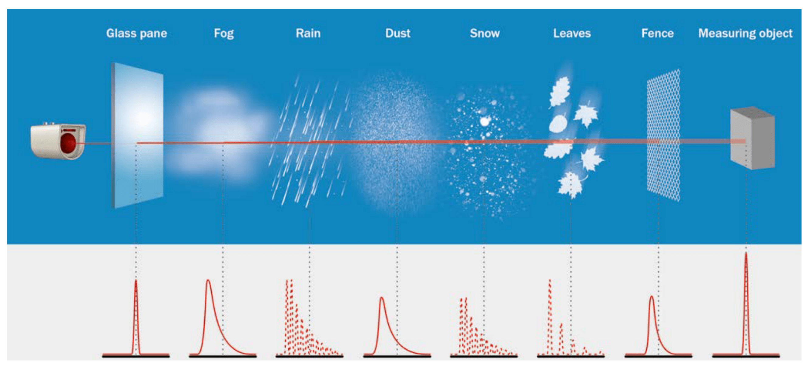
Autonomous driving relies on strong perception capacities, as a precise understanding of the environment around the vehicle is required. Significant progress has been made in this field, enabling autonomous vehicles (AVs) to evolve in a large variety of environments, but there remain difficulties in the presence of adverse weather conditions. Daily climatic phenomena, such as rain, snow or fog, impact the sensor data, which alters the algorithmic methods required by autonomous navigation (detection, localisation). To handle these issues and propose solutions, one should have a good insight into the consequences induced by these water particles on the sensors’ signals.

Depending on the wavelength, sensors’ signals are influenced by scattering and absorption effects. Radar sensors use millimeter waves and are less impacted than optical sensors by fog as their wavelength is larger than the fog particles’ diameter, and are relatively less impacted by rain and snow. However, automotive radars have lower resolutions than lidars and higher levels of noise, which increases in DVE [1]. Similarly to human vision, passive sensors in the visible spectrum are affected by raindrops, snowflakes and fog clouds, altering the recognition of objects by reducing contrasts and increasing the number of white pixels. Cameras using infrared spectral bands have different behaviors: thermal bands allow for better penetration in fog conditions, but still suffer from strong contrast reduction in rainy and snowy conditions [2]. As for lidars, their data are impacted as much as visible and close infrared cameras, because they operate at similar wavelengths. The emitted photons are scattered by the water droplets, whether they are liquid, solid, falling or suspending.

1.2. Lidar Signal

A lidar sensor sends laser beams towards the environment and collects the photons returning towards the sensor after backscattering. In the case of a pulsed emission (the most common technology for autonomous vehicles), the beam is slightly divergent: when a laser shot propagates in a scattering medium, the resulting signal on the detector is a combination of the proportions of light returned by the various impacted objects. In addition, the absorption and scattering of light in the atmosphere, as well as ambient light noise, contribute to the resulting signal on the detector. The whole returned signal is called the full wave form (FWF). Unless the system is capable of returning this FWF signal to the user, an internal signal processing algorithm analyzes the signal and returns digitized echoes (Figure 1).

In most automotive lidars, the time-of-flight (TOF) principle is then applied to estimate the distance between the sensor and the objects from the elapsed time between the emission of the photons and their backscattering on objects. The detected ranges and orientations of the laser beams (elevation and azimuth) result in 3D coordinates of impacts in the sensor reference frames, and the combination of all 3D impacts gathered during a scanning period produces a 3D-pointcloud (Figure 2).

In this work, we only consider digitized echoes as the lidars currently available for autonomous driving (COTS systems) do not provide access to the FWM signal and directly output pointclouds. The maximum number of echoes delivered for each laser shot depends on the considered device. For lidars that only output a single echo, this echo is either the strongest return (higher quantity of returned light), which most likely corresponds to a real target rather than noise, or the last return, which does not take into account in-between echoes. Lidars that have a multi-echo capability yield a more accurate representation of the environment, but also a larger amount of points coming from water particles and a bigger data volume. Figure 3 exhibits the various possible echoes on a FWF return in a DVE situation.

1.3. Contribution and Outline

This study focuses on lidar sensors and aims at assessing detection rates in DVE compared to nominal data acquired in clear conditions. We are also interested by the possibility of using lidar data to infer properties on the environmental weather conditions, which could lead to the estimation of the DVE properties.

We performed extensive experiments in an indoor climatic chamber, in which various rain and fog conditions have been generated. We recorded data acquired by a group of lidars on a static scene, and analyze the echoes’ intensity and the number of 3D points corresponding to a specific target, as well as the data corresponding to the space between the sensors and the target (the frustum). Our goal is to assess the degradation of objects’ detection as a function of the rain and fog characteristics for the considered sensors.

Section 2 reviews related works. Section 3 presents the experiments’ setup and the complete set of sensors used. Section 4 describes the considered methodology for both the generated weather conditions and the analysis of the results. Section 5 then presents the results by comparing the sensors using the same and repeatable DVE. Finally, a discussion about the difficulties related to artificial rain generation is proposed in Section 6, along with a comparison of the different sensors’ performances and their potential explanations.

2. Lidar Sensors in DVE

The popularity of lidar technology for AVs has been rapidly growing since the DARPA challenge in 2003 [6] but there are some limitations in the presence of DVE that alter the data and thus reduce the safety and availability of these systems [7,8]. Various works study sensors’ performances in adverse weather conditions; some are related to the physical principles at the origins of the limitations [9,10], while others rely on experiments and assess sensor behavior in real or artificial conditions [11,12,13,14,15,16,17]. Michaud et al. [11] show different spinning lidars (e.g., constructors Velodyne, SICK and Hokuyo) behaviors in front of snow conditions by positioning them on a building window, aiming at the snow-covered ground. Studying the distances of the detected snowflakes, they state that the probability of detecting a snowflake is a log-normal or sum of log normal distributions. In [12], a Velodyne VLP-16 spinning lidar is used to analyse different road objects (e.g., asphalt, cones, signs, walls) in various rain conditions. The evolution of range, intensity and number of points on the targets is presented with increasing rain intensity. It showcases a degradation of the perception performances of the sensors, especially on the number of points on the targets in the 3D-pointclouds. Refs. [11,12] performed outdoor acquisitions where it is hard to record repeatable weather conditions unless a complete static recording setup is available and data should be recorded for a large period of time. To build a consistent dataset, additional context sensors are needed to measure the characteristics of the DVE: rain intensity in mm/h, snow-water equivalent (SWE) in mm or fog visibility in m, which can be measured by transmissiometers or scatterometers for fog, disdrometers and rain gauges or SWE sensors for rain and snow, respectively.

Refs. [13,14,15,16,17] all present results produced in an indoor climatic chamber available at Cerema (“Centre d’Etudes et d’expertise sur les Risques, l’Environnement, la Mobilité et l’Aménagement” in French) in Clermont-Ferrand, France. This platform can be used for testing perception sensors in adverse weather conditions and carrying out experiments in a controlled environment so as to ensure the repeatability of weather conditions. Kutila et al. [13] measure the attenuation induced by fog for the Ibeo Lux sensor and a custom 1.55 µm lidar, which is supposed to show better performances because eye-safety regulations allow for a higher power emission at this wavelength [10]. This latter study demonstrates similar signal attenuation between the two sensors, thus the use of a higher power emission is very likely to improve the signal-to-noise ratio (SNR) and hence the overall performances. The behavior of Velodyne HDL64-S2 and HDL64-S3 lidar sensors in artificial fog conditions is studied in [14]. They showcase different performances depending on fog densities, multi-echo capabilities and power levels of laser emission. Various lidar sensors working around the standard 905 nm wavelength are used by Jokela et al. [15], including mechanical beam steering Ibeo Lux, spinning Velodyne, Ouster and Robosense and resonant oscillation based micro-motion technology (MMT) Cepton sensors. Their study focuses on the variation of range measured by the sensors in artificial fog and a qualitative analysis of the pointclouds degradation in natural snow conditions. SVM and kNN machine learning algorithms were considered in [16] to classify weather conditions from Velodyne VLP-16 and Valeo Scala lidar sensors. They use a feature vector that includes geometric properties of the pointcloud as well as intensity and multi-echo information. The study shows a good performance using the Velodyne sensor and support vector machine (SVM) learning model. Li et al. [17] study the impacts of fog conditions on detections from a Velodyne lidar aiming at different targets. The generation of complete fog dissipations allow them to record continuous evolutions of the signal degradation. A Gaussian Process Regression machine (GPR) learning approach is finally proposed to measure the disappear visibility of the different objects. Despite limitations on the similarity with natural conditions, artificial rain and fog generation is practical due to the possibility of having repeatable and controlled weather conditions.

Table 1. Synthesis of experimental analyses of lidars in DVE.

Sensors	Experimental Conditions	Metrics	Further Analysis
Ref. [11] Hokuyo UTM-30LX-EW SICK LMS200 SICK LMS151 Velodyne HDL-32E	Natural snow	Detected range Detected beam angle Proportion of snowflakes echoes Spatial distribution	Statistical approach Bayesian framework about spatial distribution of echoes
Ref. [12] Velodyne VLP-16	Natural rain Multiple urban surfaces	Range Number of points Intensity	∅
Ref. [13] Hello-World 1550 nm Velodyne VLP-16 Ibeo Lux	Artificial rain Artificial fog Various reflectivity targets	Signal attenuation Pulse Width Intensity	Confrontation of 905 nm and 1550 wavelengths
Ref. [14] Velodyne HDL-64 S2/S3 Ibeo Lux/HD	Artificial fog	Maximum viewing distance Number of points Intensity	Emitted power levels Quality of scanning patterns Multi-echo capabilities
Ref. [15] Ibeo Lux Velodyne VLP-16 Ouster OS1-64 Robosense RS-32 Cepton HR80T/W	Artificial fog Natural snow Various reflectivity targets	Range variations Qualitative analysis of pointclouds	∅
Ref. [16] Velodyne VLP-16 Valeo Scala	Artificial rain Artificial fog	Intensity/Pulse width Number of points Spatial distributions Multiple echoes	Range Weather classification SVM & KNN
Ref. [17] Velodyne VLP-32	Artificial fog	Range Intensity	Gaussian process regression to access minimum visibility of objects, extended to [18]

summarizes the main elements of each article.

3. Materials

3.1. Generating Artificial and Controlled Weather Conditions

Our data were gathered in the Cerema 30 m long chamber, in which artificial rain and fog in night or day conditions can be produced [19]. The top cover of the chamber can be removed so as to let the sunlight in, yielding daylight conditions, or set to emulate night conditions. Light spots can illuminate the scene, shown in Figure 4. The whole facility is composed of the greenhouse and a tunnel where the weather conditions are produced and a control room where acquisitions are monitored. Rain and fog conditions are produced with a combination of nozzles (or injectors, or sprinklers) disposed on the ceiling of the chamber at about 2.10 m heigh. Specific nozzles and pressure configurations are set to produce the desired precipitation intensity (in mm/h) or fog visibility (in m).

The assessment of the condition is different for fog and rain. For fog, the chamber is equipped with a transmissiometer, a sensor that measures the optical visibility at a specific wavelength. For rain conditions, the intensity (or rate) is not measured but estimated knowing the water flow rate inside the tubes and the surface of the room. In addition, the production of rain is done with a pump system located between the tunnel and the greenhouse, allowing the distribution of water more equally in the nozzles. Fog, on the contrary, is generated by a pump system located around the control room, which leads to a unidirectional repartition of the fog in the nozzles, from the control room to the end of the greenhouse. We have witnessed that fog production leads to a non-homogeneous repartition of the fog inside the chamber.

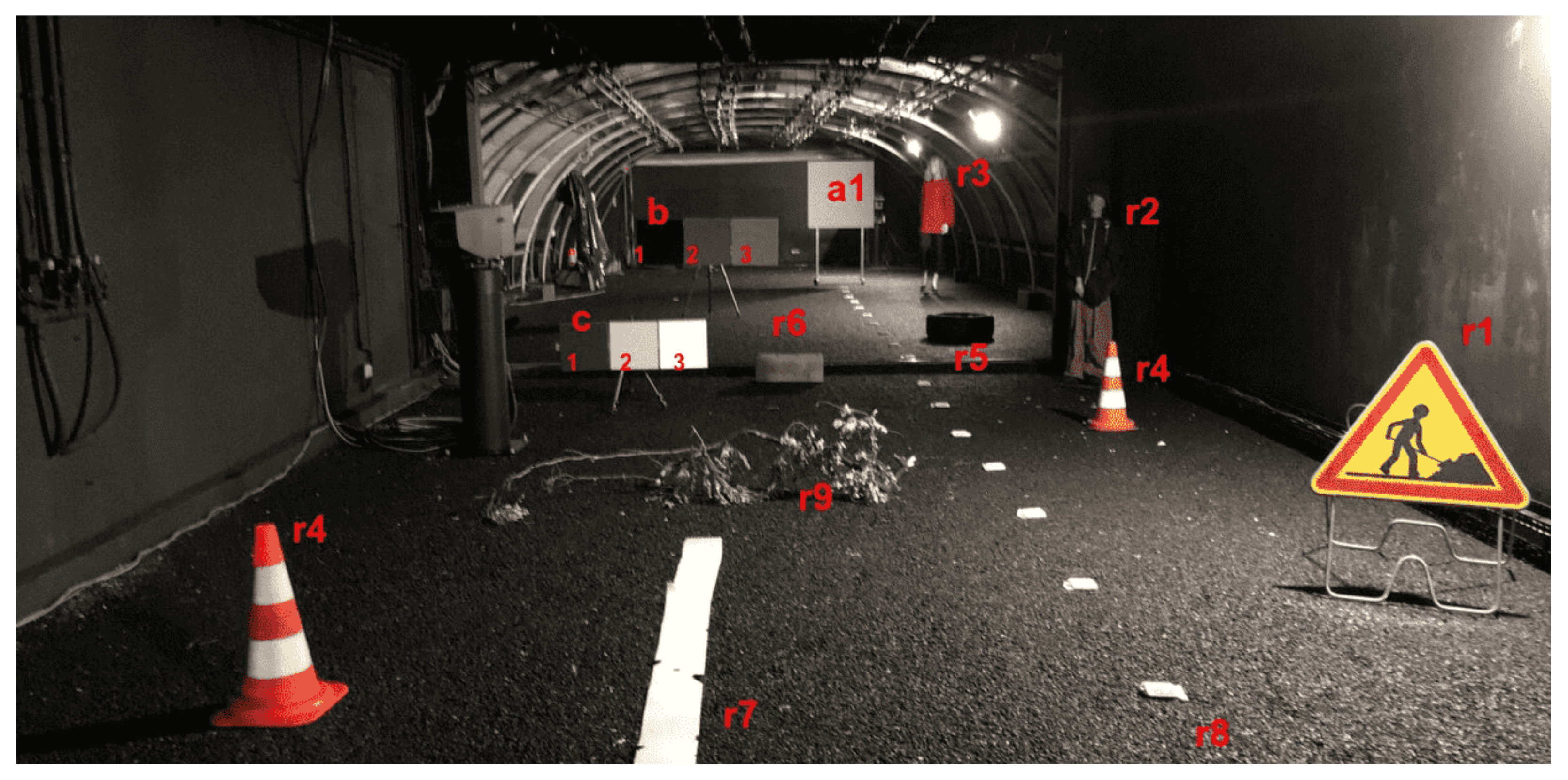
3.2. Scene Description

Figure 4 presents the different targets that constitute the static scene used in the experiments. Some targets are typical of urban road environments, others are Lambertian calibrated targets.

Table 2. List of targets used during the experiments.

Type	Objects	Reflectivity	Distance (in m)	Label
Lambertian Surfaces (Flat squares)	1 m × 1 m	80%	23	a1
	50 cm × 50 cm	10% 50% 90%	11.3	b1 b2 b3
	30 cm × 30 cm	10% 50% 90%	17.3	c1 c2 c3
Road objects	Road sign Boy dummy Woman dummy Road cones Tire Concrete Lane Beacons Tree branch	High unknown unknown High on stripes Low Low High High unknown	8 12.5 21 6.5 and 10.7 15.5 12.5 0 → 7 0 → 23 8	r1 r2 r3 r4 r5 r6 r7 r8 r9

describes these targets with their respective reflectance properties and distance to the sensors.

3.3. Lidar Sensors

A total of five lidar sensors was gathered for the campaign, namely: Velodyne VLP-32, Ouster OS1-128, Livox Horizon, Cepton 860 and AEye 4SightM. They all have different characteristics; we explain their technologies and discuss their potential differences when it comes to DVE. Deeper explanations of the technologies used for lidar systems are available in [20,21].

Table 3. List of lidars used during the experiments.

Sensor	Type	Maximum Echo Number	Wavelength (in nm)	Points in Single Scan	Intensity (in bit)
Velodyne VLP-32	Spinning	2	905	35 k	8
Ouster OS1-128	Spinning	1	850	255 k	16
Livox Horizon	Risley prisms	2	905	25 k	8
Cepton 860	Micro motion	1	905	30 k	8
AEye 4SightM	MEMS	4	1550	22 k	16

summarizes the different lidar sensors used in this experiment.

Note that we focus in this study on the weather influence on the data generation, but not on the artifacts caused by droplets on the front faces of the sensors—another issue that requires a specific approach [22]. In all our experiments, the sensors are protected and free of direct water contamination.

• Livox Horizon [23]

Working at 905 nm, this lidar makes use of Risley prisms to steer its laser beam and generate non repetitive scan patterns. It produces two echoes with an 8 bit intensity. The scan pattern changes over time in a cyclic design so that, after a certain amount of time, the totality of the FOV is scanned [24]. Contrary to spinning lidars, over time, Risley prisms lidars scan the whole environment when they remain static. It has been observed that lidars based on Risley prisms used in military systems are more efficient in DVE like dust clouds for helicopter landings or foliage penetration [25,26,27].

Figure 5a,b shows the comparison between a single scan of a Livox pointcloud (Figure 5a) and the same scene but with a temporal accumulation of several seconds (Figure 5b). The accumulation of Livox pointcloud increases the coverage of the scene within the FOV.

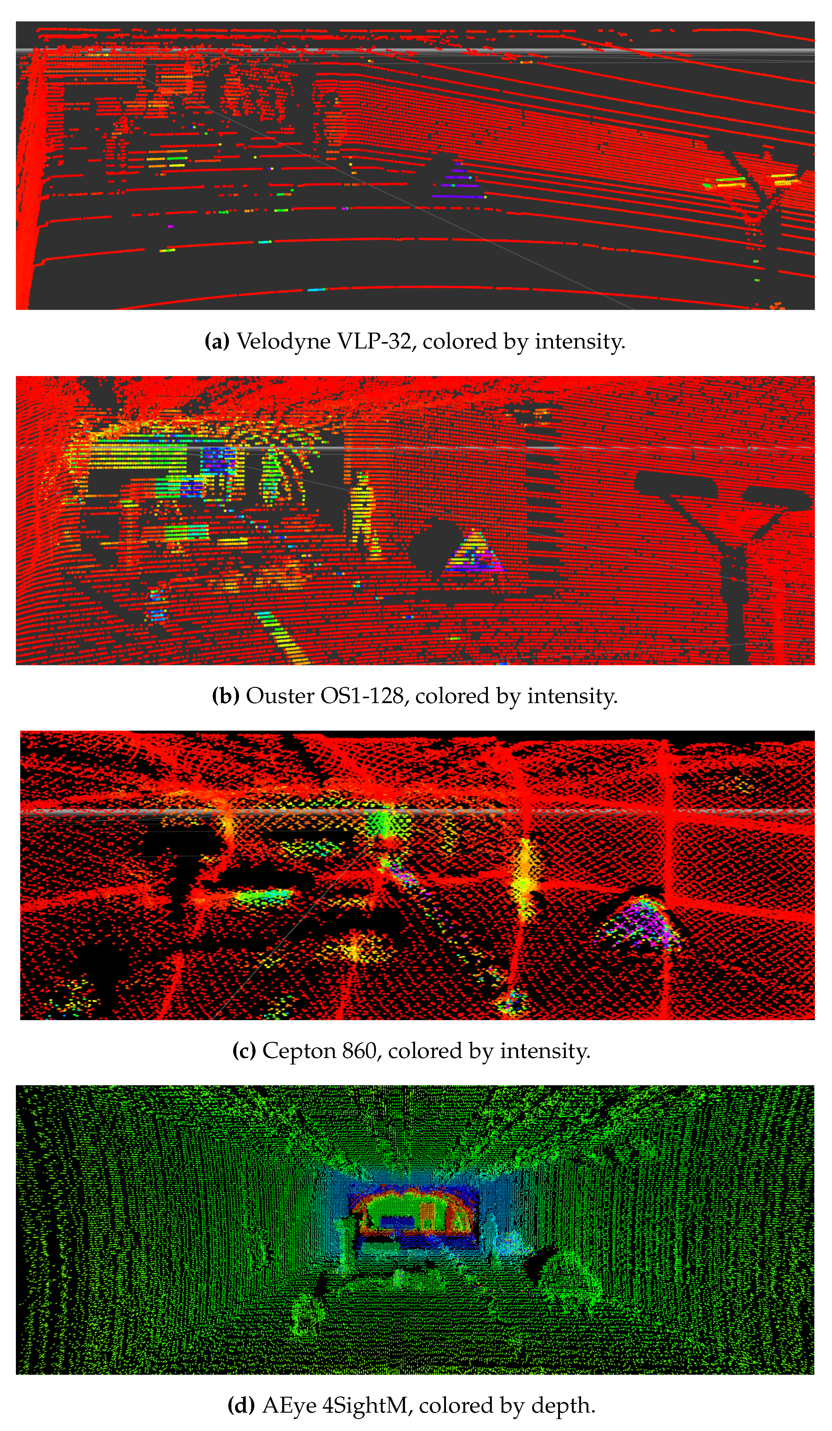
• Velodyne VLP-32 [28]

This sensor is a 32 layers 905 nm laser spinning lidar with avalanche photodiodes (APD) receivers. To produces two echoes from one single laser shot, their intensity is coded on 8 bits.

• Ouster 128 [4]

Also spinning, it uses 850 nm VCSEL lasers and single photon avalanche photodiodes (SPAD) as detectors, also known as Geiger-mode APD. Compared to the VLP-32, its 128 layers offer higher density pointclouds. It only returns one echo, the intensity of which is coded on 16 bits.

Figure 6a,b shows the pointclouds of these two spinning lidars. Visually, the only difference is the number of vertical layers. The sensors being static and the scanning pattern fixed, some areas are never scanned.

• Cepton 860 [29]

Cepton sensors work with a unique technology based on micro motion (MMT). The 860 sensor uses 905 nm laser emissions. The model we use has single returns, whereas the latest version supports dual returns. The sensor is composed of 24 channels (each channel is a laser-detector pair) in an optical module and the module as a whole is subject to frictionless oscillation to generate a 3D image across a FOV. Figure 6c shows a Cepton 3D-pointcloud colored by intensity. The 24 channels overlap on the edges to avoid empty scanned spaces. Cepton sensors have stable performances in range variations when it comes to adverse weather conditions [15].

• AEye 4SightM [30]

The AEye lidar uses a MEMS mirror to steer a 1550 nm laser beam and its detector is a Focal Plane Array (FPA). A FPA is an array of pixels performing the TOF measurements for each pixel, as opposed to single pixel architecture. This wavelength is supposed to be more efficient in adverse weather conditions due to the fact that more power can be emitted by the laser while staying eye-safe [10,13]. The sensor is capable of producing four echoes from a single laser emission. A study of MEMS mirrors for lidars is given by Wang et al. [31].

3.4. Weather Sensors and DVE Control

In addition to lidars, context sensors provide information on the characteristics of DVE. It is essential to have such instruments to gain precise information on the environmental conditions. For this purpose, we used a Parsivel disdrometer and a transmissiometer available in the climatic chamber.

• Parsivel OTT Disdrometer [32]

This sensor is capable of measuring the size, number and speed of water-droplets in rainy conditions. Other properties of the precipitation can then be derived such as the intensity of the precipitation in mm/h, the Particle Size Distribution (PSD) or the visibility. This instrument has a minimal sensitivity of 0.2 mm in diameter, which means that it cannot detect particles below this threshold [33], especially fog droplets (around 0.001–0.02 mm). It uses a static emitter-receiver laser system. The only information available about rain in the climatic chamber is the precipitation rate: the disdrometer provides precise knowledge about the droplets diameter and speed. However, it is designed to measure natural rain, and our artificial conditions can mislead the sensor. For example, changing the nozzles’ configuration to obtain certain precipitation intensities modifies the experimental conditions for the disdrometer if it remains at the same position. Considering the height of the nozzles, rain droplets are not likely to reach a stable state, as opposed to natural conditions [34]. Figure 7 shows a diameter and speed histogram of rain particles inside the climatic chamber under 120 mm/h of artificial rain rate.

• Transmissiometer

A transmissiometer is an active sensor that measures the extinction coefficients of light at a specific wavelength, usually 550 nm. Figure 8 shows the evolution of the visibility measured by the transmissiometer during fog dissipation. At first, the chamber is saturated with fog, the visibility drops to almost 0 m. Then, the fog dissipates over time and visibility increases.

• Passive cameras

The passive visible camera, Blackfly GigE from FLIR, is also used in our experiments [35]. The sensor is not tuned for the tests, its intrinsic parameters of gain and shutter speed are automatically set. It is used to bring understandable visual context, which is useful for visually assessing the artificial DVE.

4. Methodology

Setting up multiple lidar systems looking at the same scene can cause direct or indirect cross-talk between the sensors and produce artifacts in the pointclouds, thus leading to undesired measurements [36]. To avoid such phenomena and to achieve the most consistent results, the sensors are powered one by one so that they are recorded individually and do not influence each other. One minute acquisitions for each sensor and weather conditions are produced. This complicates the acquisition process but is worth it compared to having biased and non repeatable results.

In accordance with the capabilities of the climatic chamber, our test procedure and schedule, acquisitions with the following weather conditions are performed:

• Clear conditions: recordings done before any weather condition is generated and dry targets.
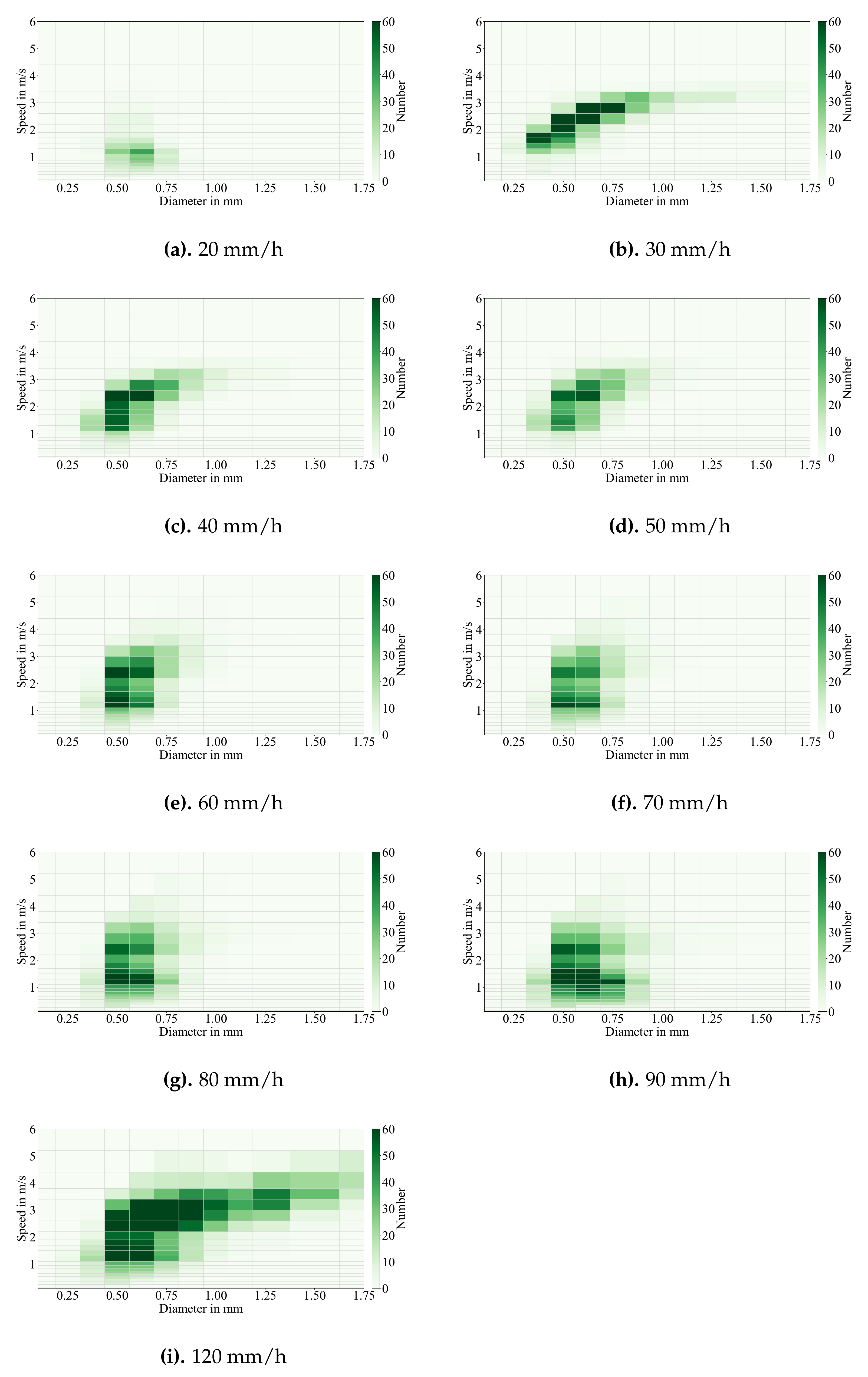
• Rain rate (in mm/h): 20, 30, 40, 50, 60, 70, 80, 90 and 120.
• Fog visibility (in m): 10, 20, 30, 40, 50, 60, 70 and 80.

The smallest rain rates are first considered here, although it is possible to produce rates beyond 120 mm/h. As lower values of rain intensities are more likely to appear in natural conditions, their study is more valuable in the context of this work. The 120 mm/h precipitation value is generated to recreate an extreme rain scenario.

Unfortunately, a mistake was made in the acquisition procedure of the AEye 4SightM sensor. As a result, only the number of points is shown for this sensor. Finally, although the Livox Horizon is capable of recording dual echoes, it was used in single echo mode during the experiments.

The data analysis is twofold: first, the evolution of the number of points and their intensity on a target is presented. This provides the first insights into the sensors’ performances and the impacts of the weather conditions on them. Second, the points located in the sensor to target frustum are studied. These data inform on the amount of noise points produced by the DVE, and on the conditions themselves. Figure 9 shows an illustration of a lidar frustum volume and associated detections in a DVE situation. The frustum is the geometrical volume between the origin of a sensor and the corners of a bounding box around a target.

From the lidar returned signal, the production of echoes depends on the configuration and capabilities of the sensor. The presence of a solid target in the path of the laser beam has a high chance of influencing the detection (or not) of noise points before this target. A real object has a higher chance of returning more energy than small objects or water particles, thus producing the strongest or the last echo. In contrast, a sensor aiming at the sky is more likely to detect noise points, as there is no obstacle to produce a strongest or last echo. If the sensor has a multi-echo capability, the effect is the same but with higher chances of returning small intensity or closer echoes. The two analyses of target returns and frustum returns are made in parallel, so as to observe the correlation between the quantity of noise in the frustum and the degradation of data on the target.

The geometric definition of the target and associated frustum is made so as not to cover the totality of the target, hence avoiding laser beams impacting the target border and ensuring that all points in the frustum come from shots aimed at the target.

5. Experimental Results

The target used is the 1 m × 1 m lambertian one, of 80% reflectivity, located at 23 m from the sensors and referred to as a1 in Figure 4. Results are presented for each generated weather condition: clear, rain and fog. They are separately described for the detections on the target and for the points inside the frustum. As can be expected, there is no point detected in the frustum in clear conditions. In order to focus on the impacts of weather conditions, all values found in the various weather conditions are normalized by the mean values found on the target computed in clear conditions, listed on

Table 4. Mean values and standard deviations of number of points on the target and associated intensities in clear conditions.

Sensor	Mean Number of Points	Std	Mean Intensity	Std
VLP-32	60.55	0.93	11.07	0.50
OS1-128	87.05	0.29	47,482.61	1268.17
Livox Horizon	51.82	4.60	104.40	4.13
Cepton 860	109.08	3.31	1.51	0.27
AEye 4SightM	62.85	1.62	∅	∅

. Since the clear weather condition is the most favorable case, this normalization results in detection values ranging between 0 and 1, which provides a rough estimate of the detection rate.

The mean number of points M on target in clear conditions can be considered a good approximation of the number of laser shots aiming at the target. For the case of the points in the frustum, the normalization is also computed using M. When the sensor produces multiple echoes (VLP-32, AEye 4SightM), the relation between the number of shots aiming at the target, the number of points on the target and the amount of noise in the frustum is not straightforward. Indeed, a single shot can produce multiple echoes in the frustum, an echo in the frustum and another one on the target or only an echo on the target, as shown Figure 1 and Figure 3. As a result, the number of points in the frustum can exceed $M\times E$, $E$ being the maximum number of echoes the sensor can produce. Finally, normalizing the intensity of the frustum points by the mean intensity of the target allows differentiation of the properties of solid objects versus noise points for potential intensity-based filters [37,38].

5.1. Clear

In this section, the results of the one minute acquisitions in clear conditions are shown. Extracted mean and standard deviation values of the number of points on target and their intensities are shown in Table 4. Compared to the other sensors, the Livox lidar presents the largest standard deviation and the lowest value of number of points. Taking into account the description in Section 3.3, this behavior can be explained by its beam steering leading to non repetitive scan patterns on the target, and thus to variability in the number of points. The Cepton 860 also shows an irregular behavior in terms of number of points on target but stands with the highest count. The high point density comes from the fact that the target was placed on an overlap area of the sensor emitter/receiver channels, which increases the number of points, see Figure 6c. The Ouster sensor has the most stable number of points. This sensor is known to be functioning with digital spinning, compared to analog spinning for the Velodyne sensor [39]. Its laser shots are triggered according to precise horizontal angles of the spinning part, thus always aiming at the same direction. On the contrary, the VLP-32 is triggered by a timer. This leads to potential variations in the heading of the lasers shots aiming at the target, thus inducing variations in the number of points. The difference in the number of points between the two spinning lidars is due to the number of vertical layers, as seen on Figure 6a,b. The AEye sensor shows a high number of points and also stable values due to its solid-state scanning methodology and FPA receiving technology. The intensity values should not be compared directly between the sensors, as differences in resolution (shown Table 3) and internal processing provides very different results for each sensor. In the analysis of the impacts of DVE, all values are normalized by the values found in clear conditions (shown Table 4). By doing so, the lidars’ behaviors can be compared to each other both in terms of the number of points and intensities.

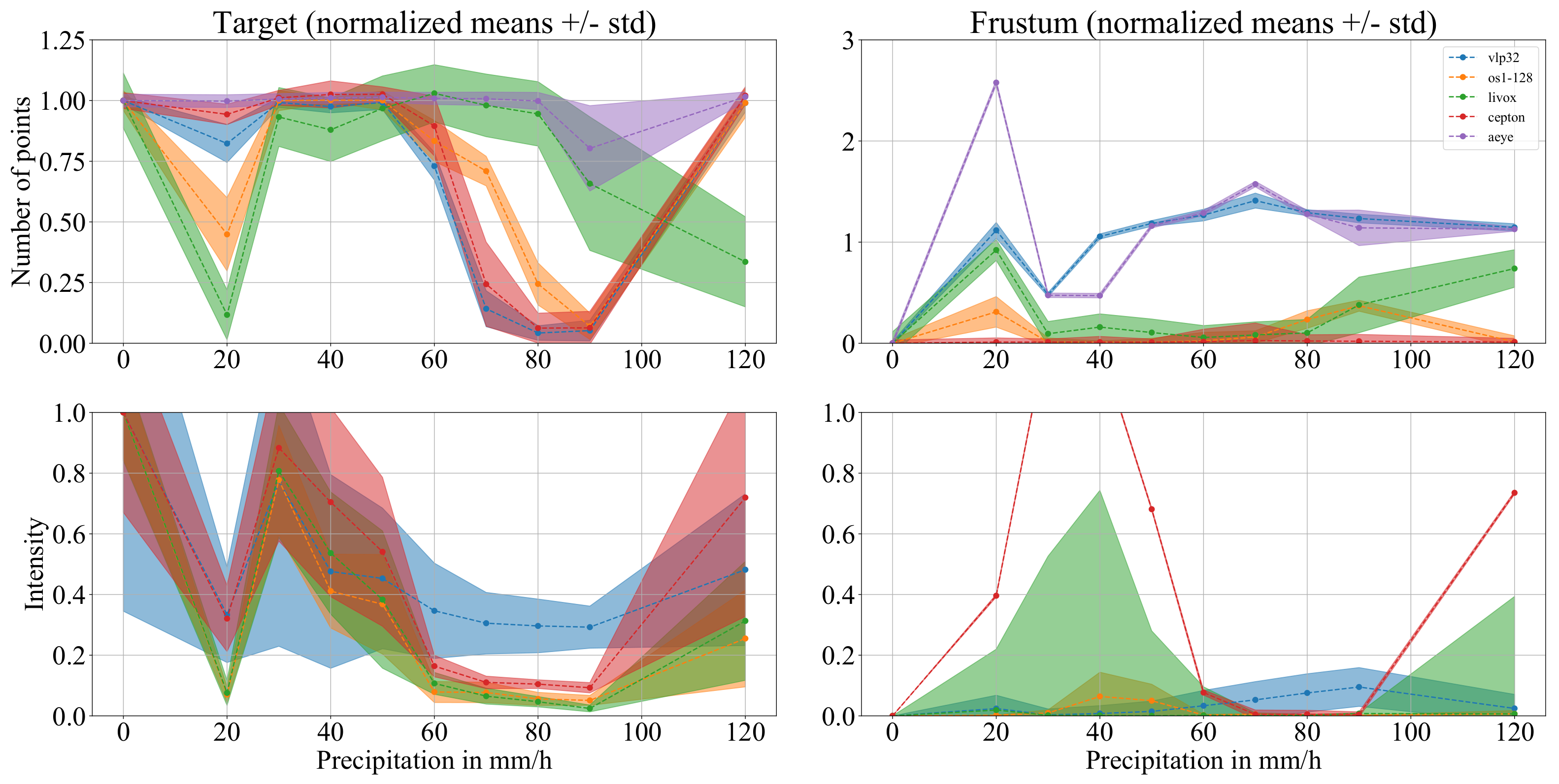
5.2. Rainy Weather Conditions

• Visual information

Images taken by the visible camera at each generated rain rate are presented in Figure 10. The images allow us to witness the evolution of visual degradation along with increasing precipitation intensity in mm/h as well as properties of the artificial rain (size of droplets, spatial distribution, spray profile)—yet one should carefully interpret these images, as they have been acquired with the camera automatic parameter control. As opposed to Figure 4, taken in clear conditions, the light spots in rainy conditions cause glare effects, caused by the scattering of light by water droplets. Comparing Figure 10a,b, one can see that the glare effect is stronger with the 20 mm/h rain rate than with the 30 mm/h one. Indeed, it is possible to see the end of the chamber at the latter while the glare effect from 20 mm/h makes the identification of objects behind target a1, a2 and a3 impossible. The observed glare effects are unexpected since an increasing rain rate would intuitively result in higher visual degradation.

Different nozzle configurations were used for these two conditions. In the first one, the first row of nozzles out of three is used. It results in droplets of small sizes, suspended in the air. On the other hand, the second row of nozzles is used for the 30 mm/h rain rate. The droplets appear bigger and seem to have higher falling speed. Rain rates up to 80 mm/h keep this last nozzle configuration but an increase in the density of the droplets inside the sprays is observable. Higher pressure and water flow rate must be set to obtain these higher precipitation intensities. Here, the size of the droplets lowers and visual degradation increases with rain rate. At 90 mm/h, the first and second rows of nozzles are activated. Visual degradation due to the glare effect is similar to results obtained under 20 mm/h rain rate although more droplets are visible. At 120 mm/h, first and third rows are activated. Visual degradation is lower than at 90 mm/h where parts of the end of the chamber can be seen due to the lower glare effect. The third row of nozzles seems to be alimented with low water pressure, thus producing bigger droplets, similarly to the 30 mm/h rain generation. The first row is activated but its effect is less significant.

• Speed-diameter histograms

The Parsivel OTT disdrometer measures the number and velocity of rain droplets. On Figure 11, the accumulation of all measurements for each generated rain rate is presented, normalized by the number of measurements. The sensor was designed to give a result every 10 s. Each graph is a 2D histogram of speed over diameter of droplets, colored by their number. Similarly to the previous results, differences are witnessed for the precipitation intensities. For example, histograms from 20 mm/h show a concentration of small diameter of (0.6 mm) and low speed (1 m/s) droplets. A tendency towards lower speeds is also witnessed. Histograms of 30 mm/h and 120 mm/h show singular properties. Indeed, in addition to having closed forms looking similar to the model of Atlas et al. [40]. these precipitation values are the only one to be correctly estimated by the disdrometer. From 30 mm/h to 90 mm/h, histograms tend to shrink to a more vertical form which means a more stable diameter value. These observations tend to argue that the rain generation is correct for rain rates of 30 and 120 mm/h but is affected by imperfections at other precipitation intensities.

The impacts produced by rain droplets at different intensities on the lidar sensors are presented in Figure 12. Results from target detection and points inside the frustum are presented. For each stabilized rain rate and sensor, a 1 min acquisition is acquired. The average values of the number of points and intensity +/− 1 standard deviation during these recorded minutes are displayed, normalized by values found in clear conditions. The abscissa is the increasing precipitation rate from 0 mm/h to 120 mm/h, with 0 mm/h being the mean values taken from clear conditions in Table 4.

• Target detection

An unexpected phenomenon is first observable for the majority of the sensors as performances at 20 mm/h and 120 mm/h present contradictory behaviors with respect to the precipitation values. Indeed, as the precipitation rate increases, one can expect to observe more impacts on the sensors data. On the contrary, at 20 mm/h, almost every sensor (exceptions are described further) shows a reduced number of points on target compared to performances with higher values of precipitation. A comparable effect can also be seen on the intensities of the points which tend to decrease as well. On the other side, at 120 mm/h, while we should have the strongest impact on our data, we observe the opposite. For almost every sensor, performances increase significantly to better values compared to behaviors at lower precipitations. These phenomena have to be investigated, they are likely to originate from the rain generation in the climatic chamber: this is discussed in Section 6.1. The target detection behaviors for each sensor are presented in more detail hereafter.

VLP-32: The sensor is capable of producing its nominal number of points on the target for rain precipitations of 30 mm/h to 50 mm/h but the target is almost lost (below 20%) for precipitation values of 70, 80 and 90 mm/h. The intensity of these points are all above 20% of the nominal value and have the tendency to slowly decrease from 80% at 30 mm/h to 30% at 90 mm/h. The 20 mm/h rain rate shows a depletion of the number of points to 80% and 40% of intensity. At 120 mm/h the sensor outputs the nominal amount of points but with lower intensities of 50%.

OS1-128: The Ouster sensor behaves similarly to the VLP-32 but the loss of the target comes later in precipitation intensity, reaching the lowest value of 10% at only 90 mm/h. However it shows greater intensity values variations: a high peak of almost 80% can be observed at 30 mm/h but the intensity decrease is more progressive and reaches almost 0% by 60 mm/h to 90 mm/h. The 20 mm/h precipitation results in a high degradation on the number of points to 40% and intensities to 10%. At 120 mm/h the sensor outputs the nominal quantity of points but with lower intensities of 25% compared to nominal values in clear weather.

Livox Horizon: The Risley Prisms sensor shows intensity values similar to the Ouster sensor. However, its performances in terms of number of points are better. The sensor produces more than 80% of the nominal number for rain rate of 30 mm/h to 80 mm/h and at 90 mm/h, the target is still detected with almost 70% of points. Curiously, it is the only one who presents lower performances at 120 mm/h, with around 30% of points, being its second lowest value after 20 mm/h, although these points have higher intensities.

Cepton 860: Cepton sensor yields good performances at 20 mm/h with almost 100% of points detected on the target, but these points have low intensities of 30%. This high quality of detection is maintained until 60 mm/h with around 80% of points. Then, from 70 mm/h to 90 mm/h, it produces less than 30% of points or even values close to 0%. At 120 mm/h, Cepton’s sensor returns its nominal number of points again. This sensor shows similar behavior to the previous sensors in terms of intensity.

AEye 4SightM: The target is detected with 100% of points for precipitation intensities from 20 mm/h to 80 mm/h and 120 mm/h. The performance only decreases to a value of 80% at 90 mm/h.

• Sensor to target frustum

Similarly to target detection, the number of points inside the frustum is unexpected for the values of 20 mm/h and 120 mm/h. In a general manner, a loss of points on target is linked to an increase of points in the frustum.

VLP-32 (dual echo): The sensor produces a high number of noise points, with more than 100% of the nominal number of points on target except for 30 mm/h. Finally, points inside the frustum have lower intensity values going up to 20% of the clear weather reference on the target.

OS1-128 (single echo): Ouster’s lidar outputs less points from the generated water particles. The number of frustum points reaches the maximum values of almost 40% for 20 mm/h and 90 mm/h. An increasing tendency for the number of frustum points can be observed, from 50 mm/h to 90 mm/h, while none of the points are detected at 120 mm/h. The intensity of the frustum points in rainy conditions is nearly 0 for all rain rates, except for 40 mm/h and 50 mm/h but too few points are detected at these conditions.

Livox Horizon (single echo): The Risley prisms sensor has a peak of frustum points at 20 mm/h of almost 100% of the nominal value. A stable stage is then observed between 30 mm/h to 80 mm/h at around 15%. For the final values of precipitation, the number of points rises to 70%.

Cepton 860 (single echo): This sensor has a very low level of noise with less than 5% of its nominal value for all precipitation rates. As a result, the observed intensities for the frustum points are considered as outliers.

AEye 4SightM (4 echoes): The four echoes capability of this lidar brings a large amount of noise compared to the other sensors. The number of noise points vary depending on the precipitation rate, with a peak at 20 mm/h and a value of 250%. We then see a rise from 30 mm/h to 70 mm/h with 50% to 150%. The frustum points finally slowly decrease in number to reach more than 100%.

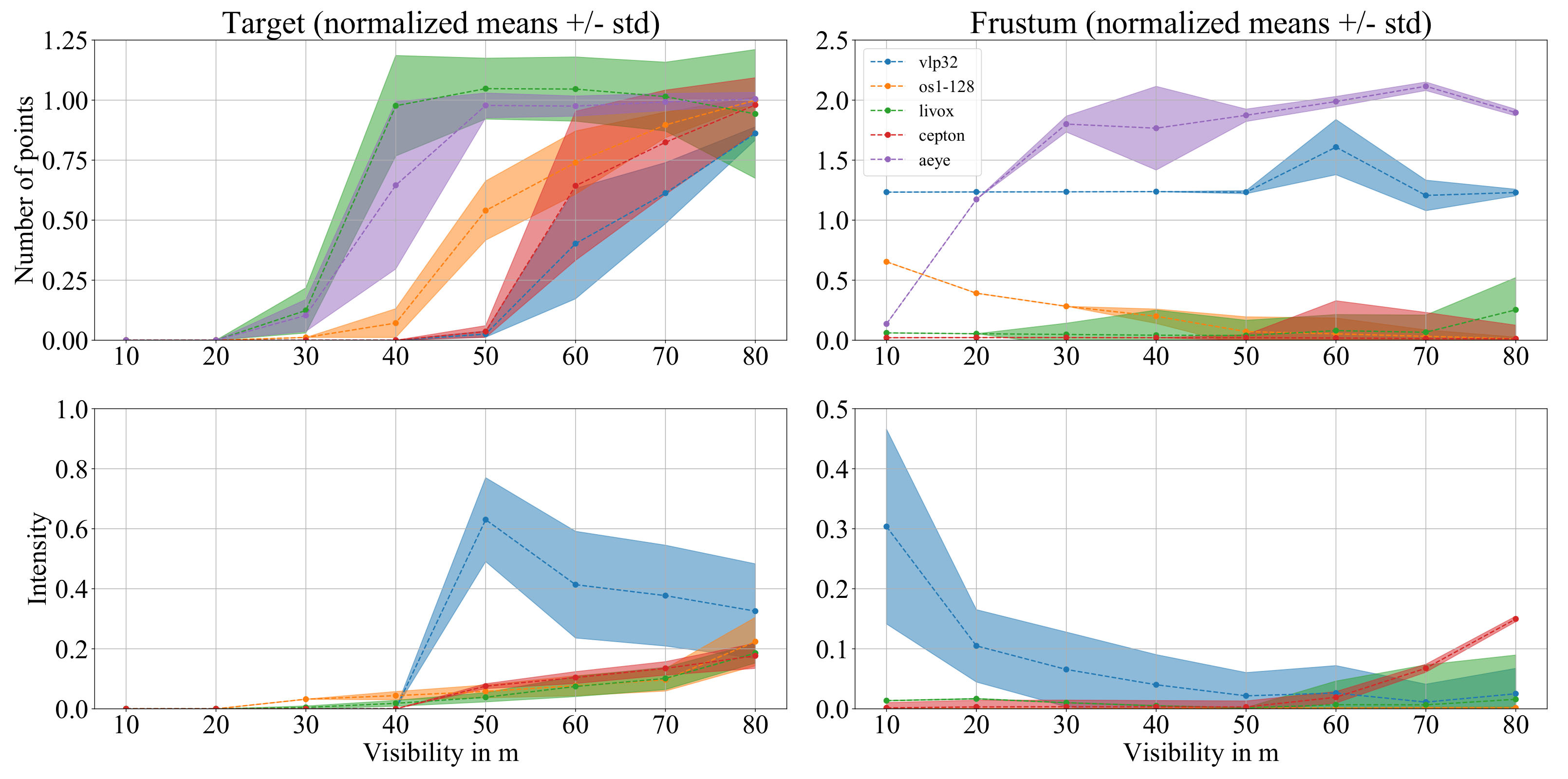
5.3. Foggy Weather Conditions

In this section, observations of the impact of fog at different visibilities on the lidars are presented. For each visibility value, a 1 min acquisition is acquired. Similarly to results given for the rainy conditions, the mean values in terms of number of points and intensity, as well as their standard deviation, are given hereafter. Here, the abscissa of the figures is the increasing fog visibility from 10 m to 80 m. Figure 13 summarizes the results for each sensor. Figure 14 shows images taken during fog experiments at visibilities 10 and 80 m.

• Target detection

In contrast to the rain impacts, getting stronger with increasing mm/h (with the exception of the rain generation problems), increasing the fog visibility here leads to a decrease in the number of fog particles. As a result, fewer impacts on the sensors data are expected as visibility increases. This can be observed in Figure 13. Contrary to the results in rainy conditions, there is no unexpected result to be reported in this case.

VLP-32: The Velodyne sensor starts to produce points on target at 50 m visibility, the number of points then rises to reach around 75% at 80 m of visibility. Its intensities have the most surprising values: starting from a peak between 50% to 80%, the values afterwards seem to stabilize around 50% as visibility increases.

OS1-128: This sensor starts to detect the target at 40 m of visibility. The number of points then rises to the maximum value of points on target for a 80 m visibility. Intensities have increasing values from 0% to around 20% at 80 m visibility.

Livox Horizon: First points appear at 30 m visibility and 100% is reached at 50 m visibility. Intensities have a rising behavior up to 20% as visibility gets to 80 m.

Cepton 860: The Cepton sensor produces its first points on target at 50 m of visibility. This number then increases almost linearly to reach 100% at 80 m of visibility. Similarly to rainy conditions, this sensor has the same performances than the OS1-128 and Livox sensors in terms of intensities.

AEye 4SightM: The MEMS sensor starts to detect the target at 30 m visibility. The number of points rises quickly and reaches 60% at 40 m visibility and 100% at 50 m.

• Sensor to target frustum

VLP-32 (dual echo): The Velodyne spinning sensor shows a quasi constant level of noise in fog conditions, at 125% of the nominal number of points on target. A curious peak up to 160% at 80 m of visibility is seen. The intensity of these points starts from 30% and goes to a reduced value of 10%.

OS1-128 (single echo): This sensor presents a decreasing number of noise points from almost 70% to 0% for increasing visibility. At all visibilities, the frustum points coming from fog stand with an intensity close to 0.

Livox Horizon (single echo): The Livox sensor keeps a low number of frustum points at around 10% and shows a slight increase for the last visibility values reaching 30% at 80 m. The intensity of these points are below 5%.

Cepton 860 (single echo): The Cepton sensor shows a very reduced number of noise points in the frustum in fog conditions, almost 0 for all visibility values. The intensity of these points is close to 0 but show a slight increase for the latter visibilities.

AEye 4SightM (4 echoes): The MEMS sensor has an increasing number of frustum points with increasing visibility. Starting from a lowest value of 25% to quickly reach around 200% at 30 m and keeping this high level of noise for the latter visibilities.

6. Discussion

6.1. Rain

Here, a synthesis of the results obtained in rain conditions is carried out, with all data presented previously (lidars impacts, visual information, speed-diameter histograms). The studied lidars show unexpected behaviors with regards to the edge rain rates of 20 mm/h and 120 mm/h. A few exceptions remain with the Livox, Cepton and AEye sensors. The former is impacted at 20 mm/h but also presents a reduced number of points at 120 mm/h along with higher intensity. On the contrary, Cepton’s lidar does not show any reduction of number of points on target at the first rain rate. Finally, the AEye sensor is not concerned with these edge cases as its target detection performances are stable across all rain rates, although its frustum detections are affected.

The reason behind these unexpected phenomena comes from the artificial rain generation. To reach a specific rain rate, a configuration between nozzles properties and water flow is used. The value in mm/h is computed accordingly using the flow rate and the room’s surface area and it results in various rain characteristics (size of droplets, spatial distribution, spray profile). Impacts of visual passive cameras and near-infrared lidars are comparable (as said Section 1.1), observations made from images in the visible spectrum can be applied to impacts on lidar data. The images of Figure 10 show different levels of degradation in the understanding of the scene. Speed-diameter histograms of Figure 11 add valuable information concerning the properties of the rain because the number of particles and their speed alter the chances of interactions with the laser shots.

At 20 mm/h, both the lidar and image data are highly degraded. The generation of this rain rate induces a large amount of small droplets in suspension, highly affecting both lidar and camera sensors. The disdrometer does not show a high number of droplets but the limitations of the sensor (described Section 3.4) should be considered as water particles may be too small to be detected, being similar to fog particles. Detections in the frustum at 20 mm/h show high numbers of noise points and sensors with multi-echo capability present the highest counts. This is in agreement with the previous observation of high number of particles at this rain rate, although not detected by the disdrometer. At 30 mm/h and 120 mm/h, while the OTT rain sensor is showing similarities with natural rain conditions and the majority of the studied lidars are not impacted in terms of target detection. Detections in the frustum show a low count of points for the prior rain rate but a relatively high one for the latter. So, it seems that artificial rain close to natural conditions does not degrade lidar data as much as less realistic rains and a higher value of mm/h (in this case of near-natural rain) means higher amounts of frustum points. When precipitation grows from 40 mm/h to 90 mm/h, the number of droplets increases but their size converges towards 0.5 mm and the resulting impacts on the lidars are intensified, although the impacts on the frustum points are not clear for all sensors. To strengthen the analysis and have a better understanding of the results at 120 mm/h, rain rates of 100 mm/h and 110 mm/h should be generated and analyzed.

The lidar sensor yielding the best performances in terms of target detection in rainy conditions is the AEye 4SightM. Indeed, almost no reduction of the number of points on target is observable across all rain rates. The higher power of emission available at the 1550 nm wavelength (while staying eye-safe) seems to allow better penetration through raindrops and thus better detection capabilities. Its four echoes capability could also be an asset in this case. Nevertheless, it is not possible to determine whether the MEMS and FPA technology of this lidar is more efficient in DVE and it makes it difficult to compare this sensor to the others working at another wavelength. We now compare the other sensors working at the common 905 nm. Both VLP-32 and OS1-128 present a similar behavior in terms of number of points on target but Ouster lidar stands with better results. Since the values are normalized their different number of vertical layers (32 vs. 128) is not sufficient to explain this difference, supposing all laser shots are independent to each others. Cepton sensor also has a similar behavior to the VLP-32 with the exception of the 20 mm/h described above where it stands with better results. Livox sensor shows more stable performances facing rising rain rate. It is able to detect the target with more than 60% of the nominal number of points at rain rates of 80 and 90 mm/h where the other sensors fail.

As expected, the only sensors with multi-echo information (VLP-32 and AEye 4SightM) have higher amounts of noise points. At 20 mm/h, the AEye sensor shows the highest density with more than twice as many points as the other sensors. The Velodyne sensor has the second highest count but remains close to the other sensors at this precipitation value. Apart from this rain rate, the two sensors show a similar amount of points coming from the generated raindrops. Although they do not have the same maximum number of echoes (two for the VLP-32 and four for the AEye 4SightM), their behavior shows a convergence to a stable value around 100%. Comparing the two spinning lidars with dual or single echo mode, multiple echoes do not seem to offer better target detection but provides additional information about the environment. The AEye lidar, with its four echoes capability, provides a high level of points coming from raindrops in the frustum while having the best detection performances on the target.

In terms of intensity, the results given by our lidars show, for most rain rates, a clear differentiation between a real target and noise points. When the target is hardly detectable, the intensity of its points becomes very low as well and it could be considered noise if an intensity-based filter is considered. Sensors seem to follow a common pattern in the intensity of the target points, which varies depending on the rain rate. It allows observation of degradations of the received signals, which is additional information, especially when target detection is optimal.

6.2. Fog

In a general manner, target detection behaviors under fog conditions are alike for all sensors. When visibility is too low, the target is not detected: the laser signals are highly scattered inside the fog clouds and never reach the detectors or even the target itself. They can also be reflected by the fog clouds and create noise points in the frustums. Then, as fog dissipates and visibility rises, lidars receive more signal leading to better target detection. Finally, all the studied sensors tend to nominal target detection performances but with different results at lower visibility values.

The Livox sensor stands with the best performances in terms of target detection. AEye lidar comes second in target detection because at 40 m of visibility, the sensor shows 60% of points on target while the Livox is already performing at 100%. For the latter visibilities, the two sensors yield nominal target detection performances. Once again, the two spinning sensors have very comparable results as their number of points is rather similar. One could say that the only difference is the starting visibility value. The behavior of Cepton’s sensor is very similar to the VLP-32, as both of them show more degradation in fog conditions. The number of noise points in fog conditions is different than with rain experiments. The Livox sensor presents a low number of points as if it is poorly sensible to fog particles. On the contrary, the sensor can be highly affected by the generated rain detecting up to almost 100% of noise points in the frustum at 20 mm/h. A rise of these frustum points for the latter visibility values is however noticed. This behavior can be explained by better automatic filtering of the backscattered signals in dense fog than in dissipated ones. The Cepton sensor does not show any noise points in fog, similarly to rain conditions.

The Velodyne sensor shows an unexpected behavior in terms of intensity for the target points with a decreasing tendency as visibility is increased. However, the intensity of its frustum detections seems to be more logical as denser fog induces higher intensity and inversely. When fog is dense, the high density of particles must act similarly to a solid object and backscatter a lot of laser light, thus increasing the intensity of the frustum points. On the other hand, multiple scattering effects that dissipate the signals must be prevalent in lighter fog situations and reduce the returning intensities. The other sensors only show the opposite. As fog dissipates, target detection is improved and the intensity of the target points rises as well for the Livox, Ouster and Cepton lidars. However, intensities of the frustum points remain very low for all visibility values, except for the Cepton sensor with the rising effect described previously.

The multi-echo capability here implies again a higher number of points but not necessarily a better analysis of the environment. For example, the Ouster sensor shows a continuous decrease of its frustum points, which could easily lead to visibility classification using a simple inference model. On the contrary, the number of frustum points of the VLP-32 is rather constant over all visibility values. The AEye sensor and its four echoes presents a growing number of noise points. It rises from almost no noise points at first to a stable value of 200% of noise points for visibility values from 30 m to 80 m. Similarly to rain conditions, the two sensors with multi-echo capability show a stable value of frustum points for the majority of visibility values. The evaluation of the frustum points for lidars with multi-echo capability does not clearly provide information on the fog conditions. To go deeper, one should look at the labelization of the echoes inside these frustum points.

6.3. Multi-Echo

In this section, we take a look at the labelization of echoes inside the pointclouds of the target and the frustum for the VLP-32 lidar sensor. As said previously, this instrument can produce two echoes from a single emitted laser beam. In addition, the labelization of echoes is done according to the intensity of the returned signal. Thus, small intensity echoes (likely to come from small objects or water particles) are labelled as second echoes (echo2, second Strongest). Inversely, solid and bigger obstacles are prone to returning more energy and have points labelled as first echoes (echo1, Strongest). Figure 15 shows the same graphs of number of points from rain and fog experiments but with the labelization of echoes 1 and 2.

Detections from the target show that, regardless of the nature of the artificial DVE (rain or fog), the solid target always returns points labelled as first echoes. Even when points are detected both in the frustum and on the target, points from the latter always remain Strongest echoes. This is interesting because one could think that when the target is hardly detectable, the sensor could be confused about its Strongest echoes. Especially in fog conditions, when we observe that the intensity of the target and frustum points can be close to each other, as shown on Figure 13.

Then, a mixture of echoes is observable for the frustum points. In rainy conditions, proportions fluctuate depending on the number of points on target, which itself varies with the rain rate. Indeed, when the target is well detected (more than 75% of the nominal number of points), first echoes constitute the target and the number of second echoes is the number of points inside the frustum. As the detection performance from the target decreases, first echoes tend appear in the frustum and we see a combination of first and second echoes. When target detection fails, most echoes in the frustum are labelled as first echoes. Here, the rain droplets become the Strongest echoes as the solid target in the line of sight does not return enough energy anymore. Foggy conditions produce similar results. Until the target is detected, all first echoes are located in the frustum while the sensor does not produce any second echo. Then, starting at 60 m of visibility, the number of second echoes rises as visibility increases and the number of first echoes decreases in the frustum. The sensor receives enough energy from the target to detect it and allows for second echoes in-between.

As said previously, the multi-echo capability of the VLP-32 does not allow it to have better target detection performances with regards to the other spinning lidar sensor. Though, the labelization of echoes provides valuable knowledge on the characteristics of the environment when looking at points located in a frustum. A next step is to acquire data from natural conditions, including context weather information and lidar pointclouds. A deeper analysis on the behavior of each laser shot (which can result on target detection, frustum detection or no detection at all) is expected to add precision. Finally, the development of an automatic DVE classification algorithm is planned. This could allow an AV to adapt its detection capabilities and dynamic behaviors in consequence.

7. Conclusions

Quantitative results from automotive lidar sensors in DVE are presented in this study, with artificial rain and fog conditions of various properties. A close look at the points detected on a reflectance calibrated target is presented, as well as points detected in the frustum between each sensor and the target. This volume allows for a better understanding of the impacts of DVE on lidars while constraining the analysis to a specific space, which can, for example, be used in tracking situations.

One should be careful in the comparison of artificial and natural weather phenomena where limitations exist. Generated conditions from climatic chambers are useful for their repeatability but weather generation methods show limitations in terms of similarity with natural weather thus limiting further developments. Future work will focus on outdoor acquisitions.

Performances differ for all sensors both in number of points and intensity and sensor specific characteristics can be observed in their behaviors. Internal designs of the lidars (aperture size, detection scheme, …) could certainly explain the performance differences, but the information needed for such analysis is hardly accessible. The analysis of the impacts of DVE regarding sensor internal designs is another interesting topic that could be considered during the conception of the sensors. Our study is agnostic with respect to these design parameters because we focused on the use of the pointclouds.

It seems that the use of 1550 nm laser emission of AEye lidar allows better penetration through obscurant media. A non repetitive scan pattern from the Livox lidar also shows good performances, especially in foggy conditions. Finally, the multi-echo capability brings additional levels of noise in DVE but especially more information for the characterisation of the weather conditions. The combined analysis of target and frustum detection plus multi-echo labelization is valuable for future automatic classification of DVE.

References

1. Hassen, A.A. Indicators for the Signal Degradation and Optimization of Automotive Radar Sensors under Adverse Weather Conditions. Ph.D. Thesis, Technische Universität Darmstadt, Darmstadt, Germany, 2008. [Google Scholar]
2. Bernard, E.; Rivière, N.; Renaudat, M.; Pealat, M.; Zenou, E. Active and Thermal Imaging Performance under Bad Weather Conditions. 2014. Available online: https://oatao.univ-toulouse.fr/11729/ (accessed on 2 June 2021).
3. YellowScan. Available online: https://www.yellowscan-lidar.com/knowledge/how-lidar-works/ (accessed on 2 June 2021).
4. Ouster. Available online: https://ouster.com/ (accessed on 2 June 2021).
5. Sick. Available online: https://www.generationrobots.com/en/401697-sick-lms500-20000-pro-hr-indoor-laser-scanner.html (accessed on 2 June 2021).
6. Thrun, S.; Montemerlo, M.; Dahlkamp, H.; Stavens, D.; Aron, A.; Diebel, J.; Fong, P.; Gale, J.; Halpenny, M.; Hoffmann, G.; et al. Stanley: The robot that won the DARPA Grand Challenge. J. Field Robot. 2006, 23, 661–692. [Google Scholar] [CrossRef]
7. Radecki, P.; Campbell, M.; Matzen, K. All Weather Perception: Joint Data Association, Tracking, and Classification for Autonomous Ground Vehicles. arXiv 2016, arXiv:1605.02196. [Google Scholar]
8. U.S Department of Transportation. Vehicle Automation and Weather Challenges and Opportunities. Technical Report. 2016. Available online: https://rosap.ntl.bts.gov/view/dot/32494 (accessed on 2 June 2021).
9. Rasshofer, R.H.; Spies, M.; Spies, H. Influences of weather phenomena on automotive laser radar systems. Adv. Radio Sci. 2011, 9, 49–60. [Google Scholar] [CrossRef] [Green Version]
10. Wojtanowski, J.; Zygmunt, M.; Kaszczuk, M.; Mierczyk, Z.; Muzal, M. Comparison of 905 nm and 1550 nm semiconductor laser rangefinders’ performance deterioration due to adverse environmental conditions. Opto-Electron. Rev. 2014, 22. [Google Scholar] [CrossRef]
11. Michaud, S.; Lalonde, J.F.; Giguere, P. Towards Characterizing the Behavior of LiDARs in Snowy Conditions. In Proceedings of the 7th Workshop on Planning, Perception and Navigation for Intelligent Vehicles, IEEE/RSJ International Conference on Intelligent Robots and Systems (IROS), Hamburg, Germany, 28 September–3 October 2015; p. 6. [Google Scholar]
12. Filgueira, A.; González-Jorge, H.; Lagüela, S.; Díaz-Vilariño, L.; Arias, P. Quantifying the influence of rain in LiDAR performance. Measurement 2017, 95, 143–148. [Google Scholar] [CrossRef]
13. Kutila, M.; Pyykonen, P.; Holzhuter, H.; Colomb, M.; Duthon, P. Automotive LiDAR performance verification in fog and rain. In Proceedings of the 2018 21st International Conference on Intelligent Transportation Systems (ITSC), Maui, HI, USA, 4–7 November 2018; pp. 1695–1701. [Google Scholar] [CrossRef]
14. Bijelic, M.; Gruber, T.; Ritter, W. A Benchmark for Lidar Sensors in Fog: Is Detection Breaking Down? In Proceedings of the 2018 IEEE Intelligent Vehicles Symposium (IV), Changshu, China, 26–30 June 2018; pp. 760–767. [Google Scholar] [CrossRef] [Green Version]
15. Jokela, M.; Kutila, M.; Pyykönen, P. Testing and Validation of Automotive Point-Cloud Sensors in Adverse Weather Conditions. Appl. Sci. 2019, 9, 2341. [Google Scholar] [CrossRef] [Green Version]
16. Heinzler, R.; Schindler, P.; Seekircher, J.; Ritter, W.; Stork, W. Weather Influence and Classification with Automotive Lidar Sensors. In Proceedings of the 2019 IEEE Intelligent Vehicles Symposium (IV), Paris, France, 9–12 June 2019; pp. 1527–1534. [Google Scholar] [CrossRef] [Green Version]
17. Li, Y.; Duthon, P.; Colomb, M.; Ibanez-Guzman, J. What happens for a ToF LiDAR in fog? arXiv 2020, arXiv:2003.06660. [Google Scholar] [CrossRef]
18. Yang, T.; Li, Y.; Ruichek, Y.; Yan, Z. LaNoising: A Data-driven Approach for 903nm ToF LiDAR Performance Modeling under Fog. In Proceedings of the 2020 IEEE/RSJ International Conference on Intelligent Robots and Systems (IROS), Las Vegas, NV, USA, 24–30 October 2020; pp. 10084–10091. [Google Scholar] [CrossRef]
19. Cerema. Available online: https://www.cerema.fr/fr/innovation-recherche/innovation/offres-technologie/plateforme-simulation-conditions-climatiques-degradees (accessed on 2 June 2021).
20. Royo, S.; Ballesta-Garcia, M. An Overview of Lidar Imaging Systems for Autonomous Vehicles. Appl. Sci. 2019, 9, 4093. [Google Scholar] [CrossRef] [Green Version]
21. Available online: https://www.techniques-ingenieur.fr/base-documentaire/electronique-photonique-th13/applications-des-lasers-et-instrumentation-laser-42661210/imagerie-laser-3d-a-plan-focal-r6734/ (accessed on 2 June 2021).
22. Fersch, T.; Buhmann, A.; Koelpin, A.; Weigel, R. The influence of rain on small aperture LiDAR sensors. In Proceedings of the 2016 German Microwave Conference (GeMiC), Bochum, Germany, 14–16 March 2016; pp. 84–87. [Google Scholar] [CrossRef]
23. Available online: https://www.livoxtech.com/horizon (accessed on 2 June 2021).
24. Liu, Z.; Zhang, F.; Hong, X. Low-Cost Retina-Like Robotic Lidars Based on Incommensurable Scanning. IEEE/ASME Trans. Mechatron. 2021. [Google Scholar] [CrossRef]
25. Church, P.; Matheson, J.; Cao, X.; Roy, G. Evaluation of a steerable 3D laser scanner using a double Risley prism pair. In Degraded Environments: Sensing, Processing, and Display 2017; International Society for Optics and Photonics: Bellingham, WA, USA, 2017; Volume 10197. [Google Scholar] [CrossRef]
26. Cao, X.; Church, P.; Matheson, J. Characterization of the OPAL LiDAR under controlled obscurant conditions. In Degraded Visual Environments: Enhanced, Synthetic, and External Vision Solutions 2016; International Society for Optics and Photonic: Bellingham, WA, USA, 2016; Volume 9839. [Google Scholar] [CrossRef]
27. Marino, R.M.; Davis, W.R. Jigsaw: A Foliage—Penetrating 3D Imaging Laser Radar System. Linc. Lab. J. 2005, 15, 14. [Google Scholar]
28. Velodyne. Available online: https://velodynelidar.com/products/ultra-puck/ (accessed on 2 June 2021).
29. Cepton. Available online: https://www.cepton.com/ (accessed on 2 June 2021).
30. AEye. Available online: https://www.aeye.ai/products/ (accessed on 2 June 2021).
31. Wang, D.; Watkins, C.; Xie, H. MEMS Mirrors for LiDAR: A Review. Micromachines 2020, 11, 456. [Google Scholar] [CrossRef] [PubMed]
32. OTT. Available online: https://www.ott.com/products/meteorological-sensors-26/ott-parsivel2-laser-weather-sensor-2392/ (accessed on 2 June 2021).
33. Guyot, A.; Pudashine, J.; Protat, A.; Uijlenhoet, R.; Pauwels, V.R.N.; Seed, A.; Walker, J.P. Effect of disdrometer type on rain drop size distribution characterisation: A new dataset for south-eastern Australia. Hydrol. Earth Syst. Sci. 2019, 23, 4737–4761. [Google Scholar] [CrossRef] [Green Version]
34. Wang, P.; Pruppacher, H. Acceleration to Terminal Velocity of Cloud and Raindrops. J. Appl. Meteorol. 1977, 16, 275–280. [Google Scholar] [CrossRef] [Green Version]
35. FLIR. Available online: https://www.flir.com/products/blackfly-gige/ (accessed on 2 June 2021).
36. Carballo, A.; Lambert, J.; Monrroy-Cano, A.; Wong, D.R.; Narksri, P.; Kitsukawa, Y.; Takeuchi, E.; Kato, S.; Takeda, K. LIBRE: The Multiple 3D LiDAR Dataset. arXiv 2020, arXiv:2003.06129. [Google Scholar]
37. Park, J.I.; Park, J.; Kim, K.S. Fast and Accurate Desnowing Algorithm for LiDAR Point Clouds. IEEE Access 2020, 8, 160202–160212. [Google Scholar] [CrossRef]
38. Shamsudin, A.U.; Ohno, K.; Westfechtel, T.; Takahiro, S.; Okada, Y.; Tadokoro, S. Fog removal using laser beam penetration, laser intensity, and geometrical features for 3D measurements in fog-filled room. Adv. Robot. 2016, 30, 729–743. [Google Scholar] [CrossRef]
39. Ouster-Digital-vs-Analog-lidar. Available online: https://ouster.com/resources/webinars/digital-vs-analog-lidar/ (accessed on 2 June 2021).
40. Doppler Radar Characteristics of Precipitation at Vertical Incidence. 2006. Available online: https://agupubs.onlinelibrary.wiley.com/doi/abs/10.1029/RG011i001p00001 (accessed on 2 June 2021).
Figure 1. Schematic FWF signals from an airborne lidar, Copyright © YellowScan [3].
Atmosphere 12 00738 g001
Figure 2. Pointcloud from Ouster lidar, Copyright © Ouster [4].
Atmosphere 12 00738 g002
Figure 3. Schematic FWF signal in DVE, Copyright © SICK [5].
Atmosphere 12 00738 g003
Figure 4. Inside of the climatic chamber during the experiments.
Atmosphere 12 00738 g004
Figure 5. Captures of pointclouds from Livox lidar.
Atmosphere 12 00738 g005
Figure 6. Captures of pointclouds taken by each sensor.
Atmosphere 12 00738 g006
Figure 7. Example of a speed-diameter histogram taken with the OTT Parsivel disdrometer under 120 mm/h.
Atmosphere 12 00738 g007
Figure 8. Visibility measured by the transmissiometer during fog dissipation.
Atmosphere 12 00738 g008
Figure 9. Schematic diagram of a lidar frustum in a DVE situation.
Atmosphere 12 00738 g009
Figure 10. Screenshots taken from rain experiments.
Atmosphere 12 00738 g010aAtmosphere 12 00738 g010b
Figure 11. Speed-diameter histograms from rain experiments.
Atmosphere 12 00738 g011
Figure 12. Sensors behaviors under rainy conditions.
Atmosphere 12 00738 g012
Figure 13. Sensors behaviors under foggy conditions.
Atmosphere 12 00738 g013
Figure 14. Screenshots taken from fog experiments.
Atmosphere 12 00738 g014
Figure 15. Results from VLP-32 with multi-echo labels.
Atmosphere 12 00738 g015