Performing Hydrological Monitoring at a National Scale by Exploiting Rain-Gauge and Radar Networks: The Italian Case

Abstract

Hydrological monitoring systems relying on radar data and distributed hydrological models are now feasible at large-scale and represent effective early warning systems for flash floods. Here we describe a system that allows hydrological occurrences in terms of streamflow at a national scale to be monitored. We then evaluate its operational application in Italy, a country characterized by various climatic conditions and topographic features. The proposed system exploits a modified conditional merging (MCM) algorithm to generate rainfall estimates by blending data from national radar and rain-gauge networks. Then, we use the merged rainfall fields as input for the distributed and continuous hydrological model, Continuum, to obtain real-time streamflow predictions. We assess its performance in terms of rainfall estimates from MCM, using cross-validation and comparison with a conditional merging technique at an event-scale. We also assess its performance against rainfall fields from ground-based data at catchment-scale. We further evaluate the performance of the hydrological system in terms of streamflow against observed data (relative error on high flows less than 25% and Nash–Sutcliffe Efficiency greater than 0.5 for 72% and 46% of the calibrated study sections, respectively). These results, therefore, confirm the suitability of such an approach, even at national scale, over a wide range of catchment types, climates, and hydrometeorological regimes, and for operational purposes.

1. Introduction

Radar data and hydrological models are useful tools to monitor, in real-time intense rainfall and the flash-flood events they frequently generate. These tools are widely used by institutions in charge of forecasting and monitoring natural disasters around the world. The role of the spatial distribution of radar data in hydrological modelling especially when isolated rainfall events occur was evidenced by [1], while in 2002 [2] described one of the first operational applications of a flood monitoring system exploiting radar data. Many hydrological nowcasting experiments and studies were possible only thanks to the availability of radar rainfall estimates [3,4,5]. The need for using quantitative reliable rainfall estimates as input in hydrological modelling systems was evidenced by [6], but uncertainties associated with radar data are often large (see [7] for a review), especially in mountainous environments [6]. One of the widely used approaches to dealing with this issue is the integration of radar data with rain-gauge data. A very useful review of methodologies for the radar–rain-gauge combination, used in order to obtain rainfall estimates that are as reliable and detailed as possible, was provided by [7]. The basic idea is to exploit the capability of radar data to capture the spatial structure of rainfall and the high quantitative reliability of rain-gauge data. Radar data are now operationally used for both rainfall-based and flow-based flash flood early warning systems, following the definitions adopted in [5] and references therein. Zanchetta and Coulibaly in [8] suggest the use of flow-based flash flood early warning systems relying on (i) radar rainfall estimates and (ii) distributed and mixed conceptually–physically based hydrological models, such as Continuum [9], in large domains covered by a radar network. Over the last decade, flood forecasting services shifted from local- to large-scale [10], and today many national [11], continental, and even global [12] hydrological modelling systems are operational in predicting floods. In Italy, a network of Decentralized Functional Centers (CFD) accomplishes hydrological monitoring, coordinated by a national institution, the Italian Civil Protection Department, and its Central Functional Centre (CFC) [13,14]. A national-scale system, like the one we present here, allows us to have a coherent overview and to monitor areas that are possibly not covered by local modelling systems. Moreover, it allows us to overcome also the issues reviewed in [10] around the decentralization of operational flood forecasting services.

In the present work, we describe and evaluate a system that monitors hydrological occurrences in terms of streamflow at the Italian scale, by exploiting rain-gauge and radar data as input for the hydrological model, Continuum [9]. We modified and applied to the data derived by national rain-gauge and radar networks the method described in [15] to generate hourly rainfall estimates. We exploited radar data to carry out a point by point parameterization of a kriging-like interpolation algorithm, and then we used them to obtain the final merged rainfall fields. We then used rainfall estimates as input to the continuous and distributed hydrological model, Continuum, in order to get streamflow estimates. Hydrological modelling chains with a similar setup (i.e., exploiting radar data and the hydrological model, Continuum) were successfully tested at an event- and regional-scale, [5,16], while this study contributes to exploring the application of such types of system on a large scale with quite fine spatio-temporal resolutions. The hydrological modelling chain here described is operationally used by the National Italian Civil Protection Department (DPC). Thus, this work contributes to showing the suitability of this approach even at a national scale, over different catchment types, climates, and hydrometeorological regimes, and for operational purposes.

2. Tools and Methods

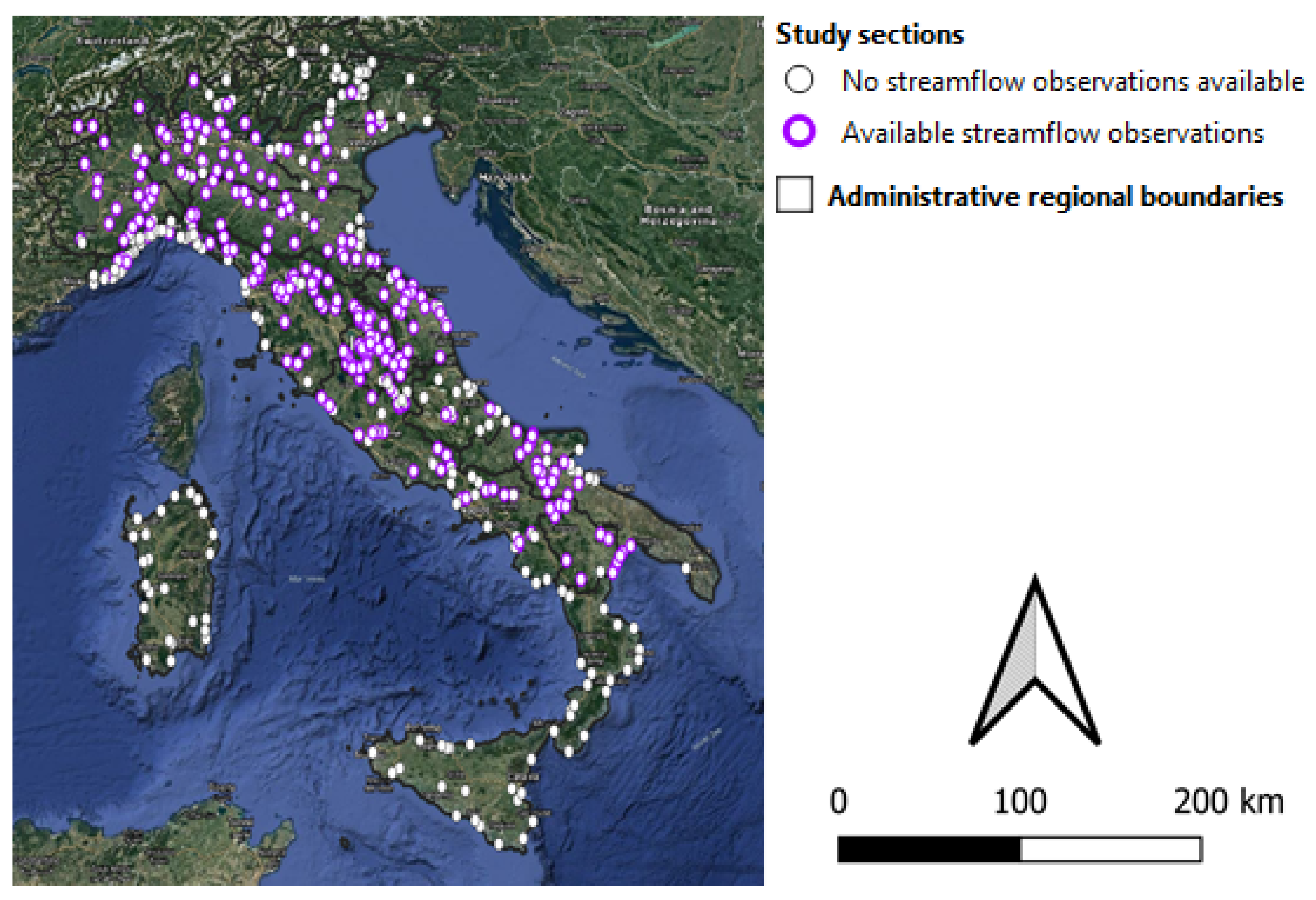
2.1. Study Area and Period

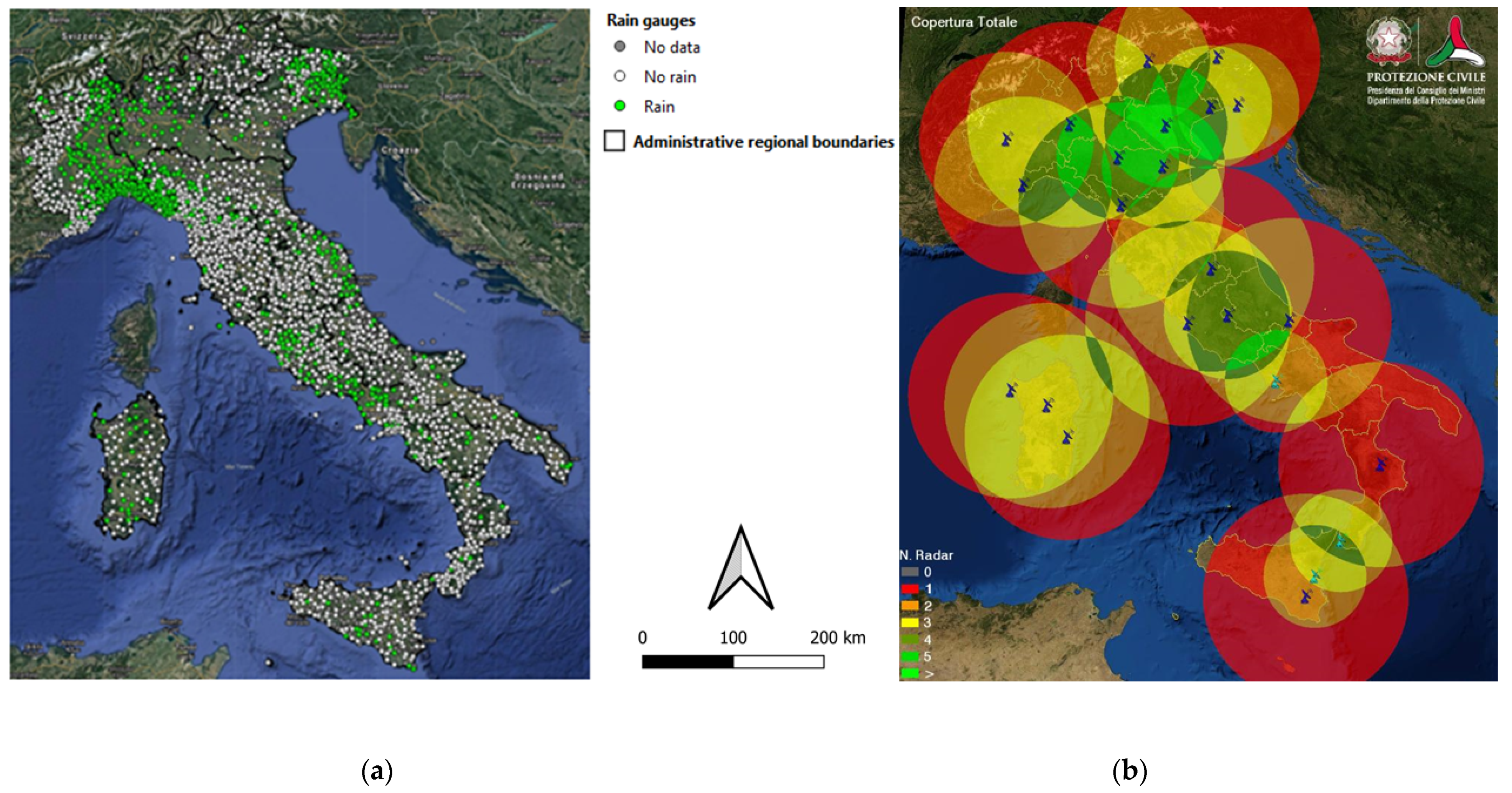
The study area was the whole of Italian, a country characterized by a wide variety of topographic areas and climatic environments that are reflected in catchment types and hydrometeorological regimes. Topography in Italy varies from mountainous along the Alps (in the north) to flat and highly urbanized in the lowlands in the northern regions and then to a predominant steep coastal orography all along the peninsular coastline. Consequently, Italy has few large catchments (with an area greater than 10⁴ km²) located in the northern and central part of the country and many small- and medium-size steep catchments (drainage areas ranging from 10¹ to 10³ km²) across the country. In the northern and north-eastern alpine and sub-alpine regions, climate is cold and temperate without a dry season [17]. While it is temperate with a dry season and arid all along the western coast and in the central and southern regions [17], with most of the rainfall in autumn and winter—a typical Mediterranean climate [18]. Consequently, annual maximum flows occur in late autumn and winter in Mediterranean regions, while during summer in the alpine ones [19], because of the snowmelt. Over recent years, Italy has faced several damaging hydrological events, such as flash floods and landslides associated with heavy rainfall events affecting its small, steep, and highly populated Mediterranean catchments [20,21] and spatially more extensive fluvial floods in larger catchments (http://polaris.irpi.cnr.it/event/, last accessed on 22 February 2021).

The hydrological modelling system proposed here is distributed and covers the whole of Italy. Results are published in real-time in a webGIS platform used as a supporting system for civil protection purposes (http://www.mydewetra.org/wiki/index.php/FloodPROOFs_Italia_Deterministico_-_Osservazioni, last accessed on 22 February 2021), in terms of a time series for 457 river sections (the study sections in the following). We chose the study sections as the outlet sections of each main catchment in the country with some additional nested sections within the bigger ones. We selected the additional nested sections according to availability of observed streamflow data and proximity with urban areas and as the outlet sections of major tributaries within the catchment. This selection led to more than 450 control sections distributed across the whole of Italy and covering a wide range of catchment types (Figure 1).

2.2. Data

In Italy, regional hydrometeorological offices oversee hydrometeorological data collection. In this study, we used rainfall data from both ground-based rain gauges and the Italian radar network, as input for the hydrological model and hourly streamflow data for its calibration and validation. All the data were provided by regional offices and collected by the DPC in near real-time for civil protection purposes and hydrometeorological monitoring over the study period, that is, from water year (w.y.) 2011 to w.y. 2019. The water year is here defined as the period from September 1 and August 31, as in [22], for an Italian alpine region, and referred to with the ending calendar year.

The rain-gauge network is composed of about 4500 stations in telemetry that record continuous measurements of rainfall accumulation and transmit them in real-time to the CFD and the CFC. The mean density of the network is 1/100 km², with the highest value of 1/50 km² along the western coast and the lowest of 1/200 km² in southern Italy (Figure 2a) [20]. The temporal resolution changes from sensor to sensor but usually is 5–10 min. The Italian radar network was established for better monitoring capabilities of atmospheric phenomena [23,24], and the consequent detection and warning of severe weather related to hydrological risks. The network consists of 23 radars, covering the whole country (Figure 2b), and whose characteristics, in terms of location, band, polarization, and range, are reported in

Table 1. Characteristics of radars composing the Italian radar network.

Longitude	Latitude	Band	Polarization	Range (km)
11.6239	44.6561	C	double	200
11.6739	45.3561	C	single	200
11.2072	46.4894	C	single	200
7.7239	45.0228	C	double	200
8.1906	44.2394	C	double	200
10.4906	44.7894	C	double	200
13.4739	45.7228	C	double	200
9.0072	40.4228	C	double	200
13.1800	42.0500	C	single	200
12.7906	45.6894	C	single	200
8.1700	40.5700	C	double	200
12.2300	41.9100	C	single	200
9.2800	45.3400	C	single	200
10.6072	43.9561	C	double	200
16.6239	39.3728	C	double	200
12.7906	42.8561	C	double	200
14.6239	41.9394	C	double	200
12.9739	46.5561	C	double	200
9.4938	39.8822	C	double	200
14.8239	37.1228	C	double	200
15.0498	37.4617	X	double	100
15.6500	38.0700	X	double	100
14.2750	40.8800	X	double	100

. The Marshall and Palmer relationship [25] is used to derive rainfall rates from radar reflectivity. Some portions of the domain are covered by more than one radar (Figure 2b), so it is possible to select a better estimate using the quality of the measures. The radar temporal resolution ranges from 5 to 10 min and QPE values are stored in pixels with spatial resolution 1 km × 1 km. Therefore, the radar network provides mosaiced products with 10 min temporal resolution and 1 km × 1 km spatial resolution.

We obtained streamflow data from (i) hourly water level data collected in near real-time by DPC from regional hydrometeorological offices and (ii) rating curves provided by regional offices and literature [26]. Streamflow data were available for 241 river sections across the whole country (markers with the violet edge in Figure 1), unevenly distributed in southern and insular regions. As data collected in near real-time, streamflow time series could show uncertainties because of multiple reasons, such as measurement errors and inaccuracy in the rating curve [27]. Furthermore, quality control is recognized as one of the main challenges in operational flood forecasting with regard to data [10], and high-quality streamflow data for calibration are fundamental for skillful modelling [28]. Nonetheless, automated procedures for streamflow quality checking, which would be advisable in large-scale studies [28], are challenging and usually not implemented in operational systems [10]. Here, we applied a three-step qualitative screening procedure to observed streamflow data, before using them for hydrological calibration/validation. The procedure consisted of (i) visual inspection of the time series to detect outliers, (ii) visual comparison among time series from nested sites, when applicable, and (iii) computation of the runoff ratio for each study section and each w.y. in the study period. We identified outliers in step (i) basing on two thresholds, manually set for each section on observed (Q_obs) and the corresponding simulated (Q_sim) streamflow time series. Observed streamflow values exceeding the threshold on Q_obs with corresponding simulated values less than the threshold on Q_sim were marked as outliers, i.e., artifacts due to measurement errors, rather than real streamflow peaks, and removed. Moreover, step (ii) was thought to verify the coherence among upstream and downstream sections, and step (iii) with rainfall input data. Obviously, steps (i) and (ii) could be improved as they were basically qualitative checks. As a result of the quality check, we assigned a score between 0 to 5 to each section (0, very unreliable observations; 5, very reliable observations). We did not fill missing values, but we did not consider w.y. with more than 6 months of missing data, both because of unavailability of data or the outlier identification and removing procedure.

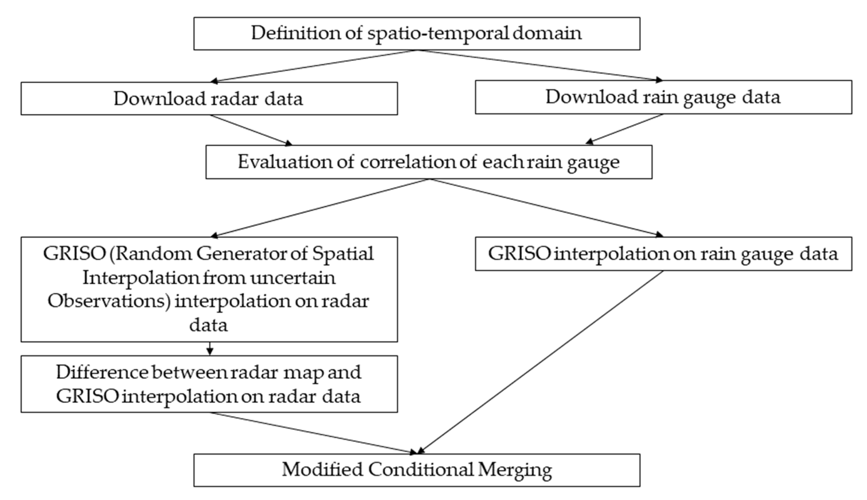
2.3. Modified Conditional Merging

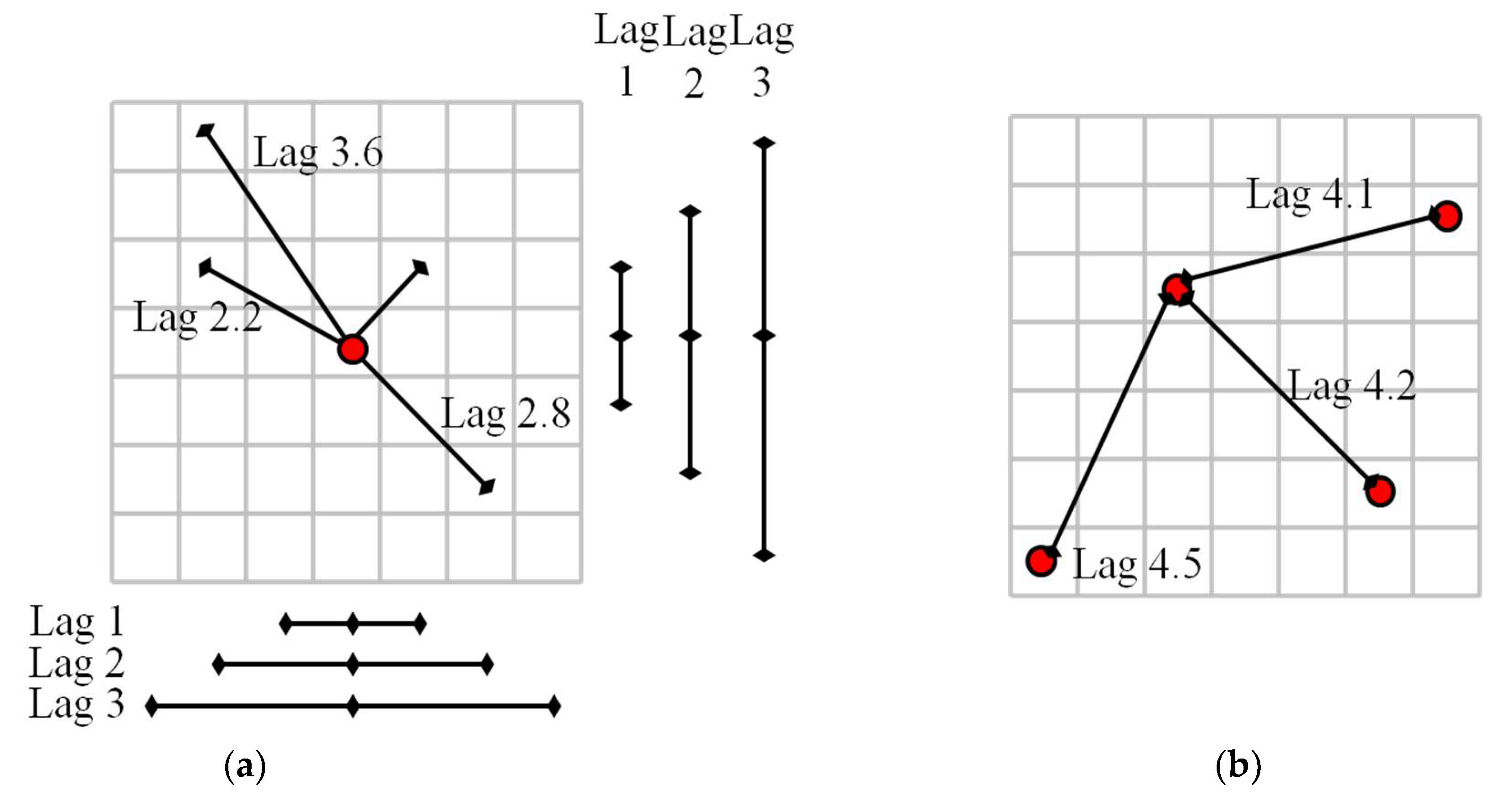
2.3.1. Description of the Method

Many studies prove that combining data from rain gauges and multispectral passive sensors represents the best way to obtain an enhanced and more reliable quantitative precipitation estimate (QPE) and the associated river streamflow [6,29]. In the last few decades, different QPE methods that combine rain-gauge and radar data have been developed following different approaches, such as geostatistical [15,30], adjustment [31], Bayesian [32], multiscale [33], and neural network [34] techniques. The choice of the most appropriate method for the specific application depends on multiple factors, such as data availability and spatio-temporal resolution [7].

Historically the rainfall observations in Italy were done by a very dense rain-gauge network (up to now with a mean density of 1/100 km²). In the last decade a radar network for a better rainfall estimation and monitoring was also set up. Both sets of data are available in real-time. Considering the spatio-temporal availability and the fact that rain gauges have good reliability but punctual observations, while radars have wide domains but with higher uncertainties (due to indirect measurement) the choice of a geostatistical approach must be the best one. Geostatistical methods are based on the evaluation of the spatial correlation of data and their goal is to evaluate the effect of the position of the measuring point on the variability of the observed data. Such variability is usually modeled by the semi-variogram, a mathematical function, which assesses the variation of the degree of correlation of points at increasing distances. The geostatistical methods get results by performing a recalibration of the field (i.e., radar map), forcing it to pass through the measuring points with certain characteristics of the covariance. Their advantage lies in the fact that they preserve the observed value in the control points, typically the rain-gauge values, which are assumed to be the more reliable evaluation of rainfall [35,36].

Sinclair and Peagram proposed the conditional merging (CM) technique [15], a geostatistical merging algorithm in which the rain gauges provide a punctual measure of the observed “real” rainfall while the remote sensors supply rainfall estimate maps which give the correlation and structure of covariance of the observed field. In fact, radar measure, even if affected by well-known sources of error (e.g., [37,38]), gives a good estimation of the general covariance structure of rainfall. Following this principle, the radar data can be used to condition the spatially limited information of the rain gauge, generating a rainfall field with a realistic spatial structure and constrained to rain-gauge values. In the CM method, the kriging is used as interpolator of the ground-based rain-gauge observations.

In this work we developed a new method that uses as starting point the CM, called modified conditional merging (MCM). In the following, a brief description of the MCM and a scheme of its workflow (Figure 3) are provided, then in Appendix A, a graphical example of the MCM algorithm is reported.

After the definition of the spatio-temporal domain of interest, radar QPEs are downloaded from the data provider (DPC) database. DPC collects polar volumes from each radar and performs some preprocess on them, including vertical adjustment, bright band correction, and clutter removal [39,40]. Rain-gauge data are also downloaded from the data provider and filtered through a spatial filter that compares each observation with the surrounding ones and removes the suspicious. The operational use reveals that the rejection rate is less than 0.05%, so there is not a significant reduction in the quantity of data. Then, the correlation is evaluated for each rain gauge (Equation (1)) and the GRISO (random generator of spatial interpolation from uncertain observations) interpolation [40,41] is performed on both rain-gauge data and radar data. For interpolation of radar data, the data are sampled on rain-gauge locations and the same parameters as for the interpolation of rain-gauge data, are used. Then, the difference between the original radar map and the GRISO interpolation on radar data is evaluated. Finally, the sum between the difference map and the rain-gauge interpolation provides the MCM map.

The novelty elements of the MCM, with respect to CM, are (i) the use of the radar rainfall field to estimate the covariance structure for each rain gauge, instead of an a priori-imposed and equal structure for every gauge, this allows a better definition of local structures; (ii) the possibility of fitting to the empirical correlation (Figure 4) a list of 3D covariance kernel (i.e., spherical, circular, exponential, pentaspherical, stable, Whittle, and Gaussian) as local structure for each rain gauge, with the consequent possibility of several different ways of spatialization; and (iii) the use of the geostatistical algorithm GRISO as interpolator, instead of kriging, for computational efficiency. Appendix B provides a short description of the GRISO interpolator.

The formula used to evaluate the correlation is:

$$R\left(l\right)=\frac{\frac{1}{N}{\sum }_i^N[P_i\left(x+l\right)-\mu \left] \ast \right[P_i\left(x\right)-\mu ]}{{\sigma }^2}$$

(1)

where $l$ is the lag or distance between points, P_i the observation of p-ith point, x the location of p-ith point, N the number of point couple at l lag distance, σ² the variance of the spatial domain where the correlation is evaluated, and μ the mean of the spatial domain where the correlation is evaluated. Obviously, the more information is available about involved lags, the better the estimation of correlation. In the MCM every pixel of the radar map is considered as a rain gauge, so it is possible to evaluate correlation for all the lags between the spatial resolution and the maximum distance for which rain gauges have influence (Figure 5a). In the case of CM, the limitation is that the correlation is estimated based on the ground-based rain gauges, that are in limited number, so the lags available for correlation estimation are few and generally similar to each other, with no information about smaller or greater values (Figure 5b) and this can lead to an inaccurate estimation of the kernel function.

The fitting of an isotropic kernel implies performing a mean of the structure that leads to a loss of information, but it results in a stable and feasible linear equation system used to interpolate. The local characteristics of the best covariance kernel (structure and length of correlation) are then used in the GRISO interpolator.

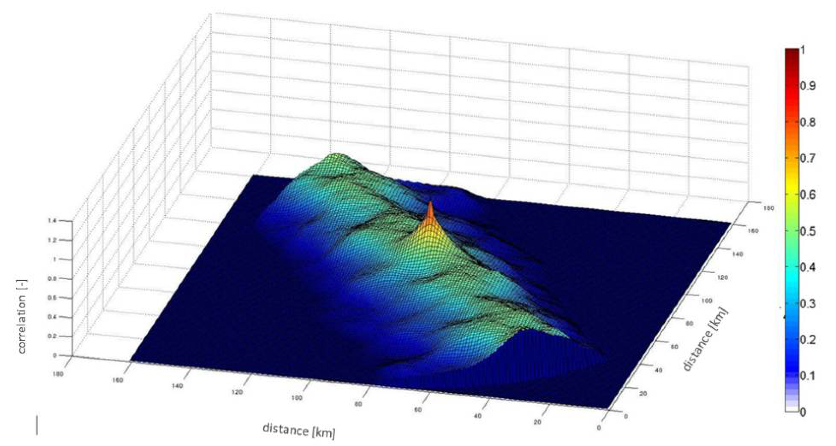
2.3.2. Analysis of Rainfall Fields

We compared rainfall fields from MCM against the ones obtained from CM algorithm at an event-scale (in the following cross-validation), in a function of the sampling density of the rain-gauge dataset. Since all the available rainfall data—from radars and rain gauges—had already been used in the MCM algorithm, we adopted a cross-validation method (i.e., sampling part of the data as input for the MCM and part as verification set). The cross-validation allowed us to have a comparison between similar data-fusion methods and, at the same time, understand the ability of the MCM as a function of network density. Then, we further compared rainfall fields from MCM against the ones obtained from ground-based data only at catchment-scale (in the following catchment-scale comparison), to verify their applicability in a large-scale hydrological modelling system, such as the one presented here. For the cross-validation we selected more than 70 heavy rainfall events according to the fulfillment of the condition of rainfall accumulation greater than 100 mm or maximum rainfall rate greater than 50 mm/h within the 2011–2014 period. They include different types of event (i.e., stratiform–convective, etc.), different accumulation times (6–24 h), different locations across the country, and different seasons. We performed a first run of the MCM algorithm using all the available data. In the cross-validation experiments the MCM algorithm evaluated the correlation for each rain gauge. Moreover, the radar observations were always used and the densities of the rain gauges were varied excluding, randomly, the 10%, 25%, 50%, and 75% of the sensors. According to the abovementioned densities, many runs of CM and MCM were performed, based on different subsets. The MCM was run using different formulae to fit the correlation. To avoid possible bad sampling and obtain stable results, 20 repetitions of the operation were performed. The temporal accumulations used were 1, 3, 6, 12, and 24 h, i.e., all the possible accumulations inside the temporal length of the selected events. We obtained 100 rainfall merged maps per time of accumulation and per type of interpolator and different statistics were evaluated on it, varying the density. The evaluated statistics are mean, standard deviation, skewness, kurtosis, the root mean square error (RMSE), the percent bias (PBIAS), the Nash–Sutcliffe efficiency (NSE) [42], and the probability density function (PDF) of the difference between maps. Moreover, the radial power spectra and the spectra along x, y directions were evaluated for each map.

Concerning the catchment-scale comparison, we computed daily areal mean rainfall time series from w.y. 2018 to w.y. 2019 for each study section (Figure 1) from (i) the MCM and (ii) the rainfall maps produced via the interpolation of ground-based data only, as the catchment-average of daily rainfall maps. Please note that we derived rainfall maps from ground-based data only after a basic quality check of ground-based sensor measurements. We performed the quality check based on thresholds of (i) rainfall intensities, to avoid outliers due to random errors, and (ii) the annual rainfall accumulation for each sensor, to exclude systematic errors because of, for instance, temporary malfunctioning. Finally, we evaluated the correlation coefficient (R) between the two rainfall estimates and then, the RMSE and PBIAS for each section.

2.4. Operational Hydrological Model at National Scale

We implemented the model, Continuum [4,9] on the whole country using the configuration described in detail in [43,44] and [21]. Basically, we employed the Shuttle Radar Topographic Mission (SRTM) DEM as a terrain model, upscaled at a resolution of 0.05° in order to have a good compromise in terms of performance and morphologic representativity. The Curve Number map was obtained through the CORINE Land Cover (http://www.sinanet.isprambiente.it/it/progetti/corine-land-cover-1, last accessed on 22 February 2021). Time resolution of the model was set as 1 h, and the update of the results was operationally done in real-time with the frequency of 1 h. In this way the available output was continuously updated exploiting the most recent observation.

Six parameters need calibration in Continuum and they relate to the surface flow, subsurface flow, and the deep flow and water table processes [43,44]. We calibrated the model following the methodology described in [43,44] on 68 sections with reliable observed streamflow data, according to the procedure described in Section 2.1. We chose the calibration period for each section as a 2-year time window over the study period, according to data availability and quality and the occurrence of high flows. In the calibration procedure we combined NSE [42] and relative error on high flows (REHF) in a multi-objective function to minimize, following the approach reported in [45]. REHF is expressed as:

$$REHF= \frac{1}{t_{max}}{[{\displaystyle \sum }_{t=1}^{t_{max}}\frac{\left|Q_m\left(t\right)- Q_o\left(t\right)\right|}{Q_o\left(t\right)}]}_{Q>Q_{th}}$$

(2)

where Q_th is chosen as the 99 percentile of the observed hydrograph along the calibration period, and Q_m(t) and Q_o(t) are the modelled and observed streamflow at time t. In those portions of territory (catchments or sub catchments) where calibration was not possible, for example because of lack of data, we set parameters according to the similarity of that portion of territory to calibrated catchments, in terms of processes involved in the rainfall-runoff transformation. As an alternative, average values of parameters are assumed. This is coherent with what done and discussed in [44] for instance.

In the operational setup, Continuum is run on hourly basis, driven by rainfall fields from the MCM to: (i) generate initial conditions, updated to the latest available meteorological observations, to run the hydrological model fed with meteorological forecast; (ii) monitor in real-time the flood events and carry out very short range forecast of streamflow; (iii) have a benchmark simulation for validation purposes, and (iv) derive climatological information in terms of streamflow along the modelled river network. Here we focus on the third objective and we use a hydrological simulation fed by MCM rainfall fields to evaluate the overall performances of the hydrological modelling system and further validate the MCM algorithm. This is achieved through the estimation of the performance metrics already used in the calibration phase on a at least 3-water-years’ time window spanning w.y. 2016 to w.y. 2019, for each study section with observed streamflow data, as done in [28,43,44].

As already mentioned, results are reported in real-time in a webGIS platform for civil protection purposes, in terms of streamflow time series for the 457 study sections (Figure 1). It is worth underling that Continuum is a distributed gridded hydrological model, so new control sections can be easily implemented in the system, for example if additional observed streamflow data become available for calibration, and this is planned. In the webGIS platform, observed streamflow data are reported for monitoring purposes as real-time data (i.e., with no quality check screening). Furthermore, skill scores from the validation exercise are also reported for each section, as useful tools in operational flood forecasting systems [46].

3. Results

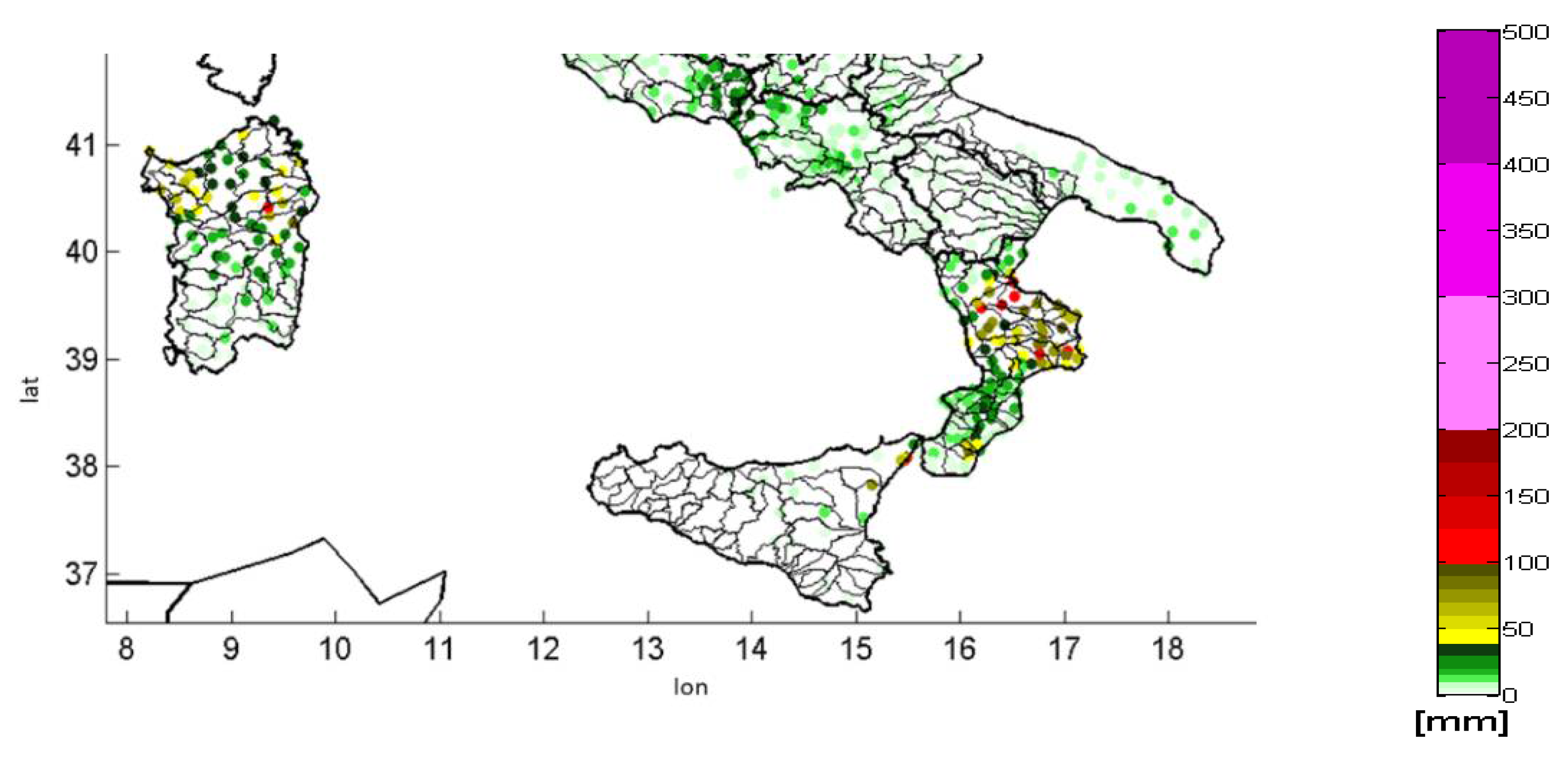
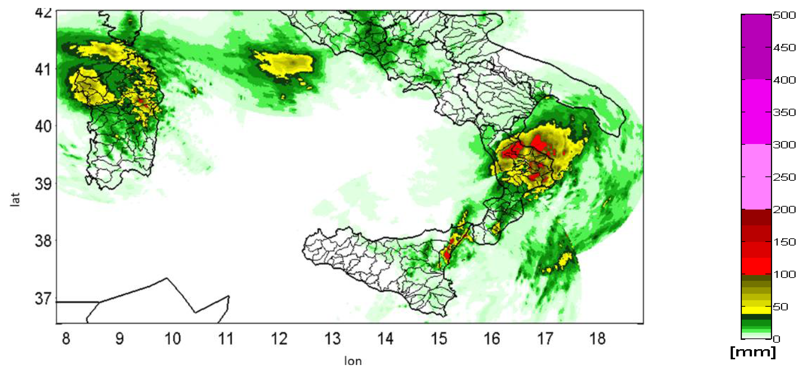
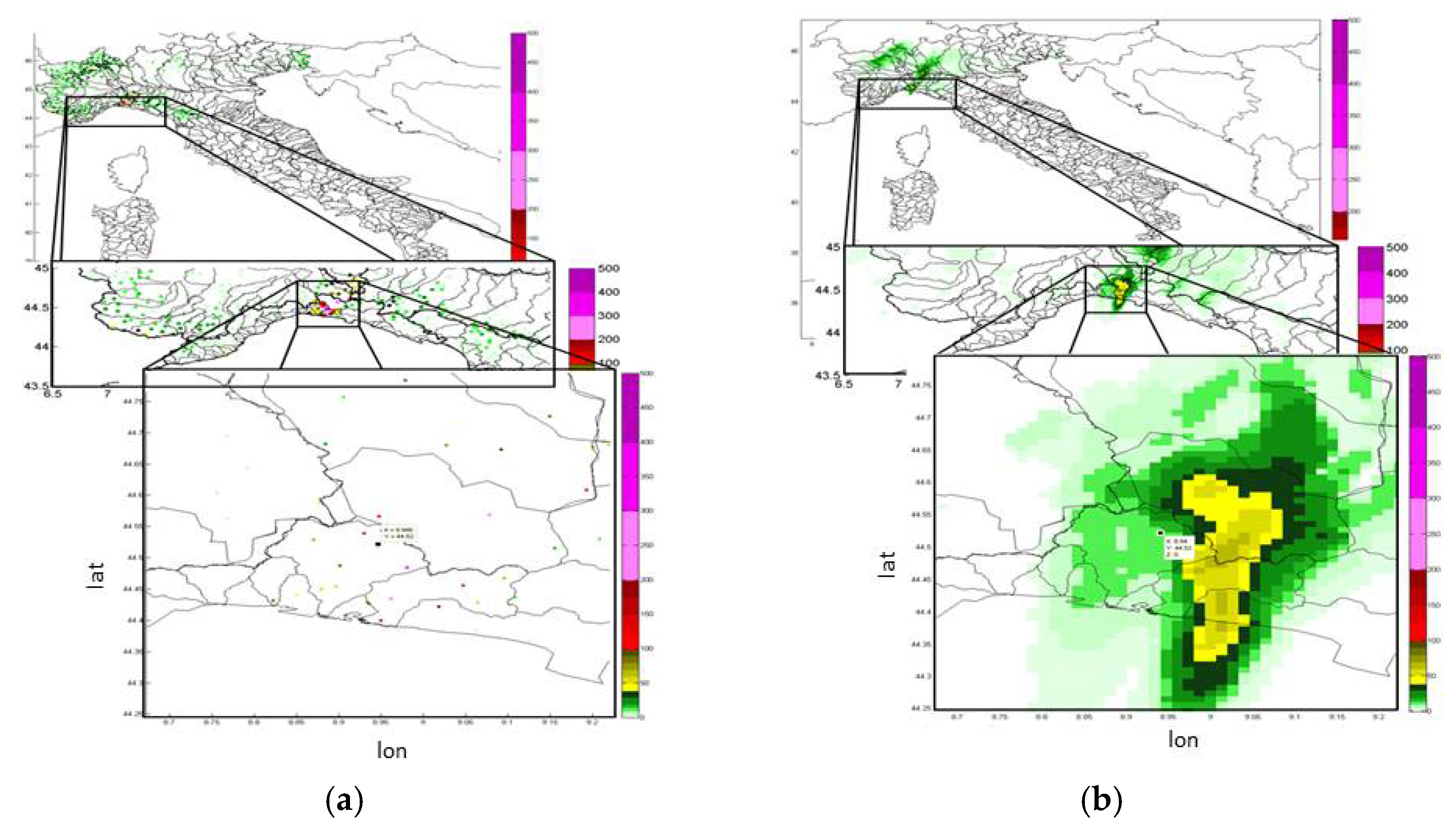
3.1. Analysis on Rainfall Fields

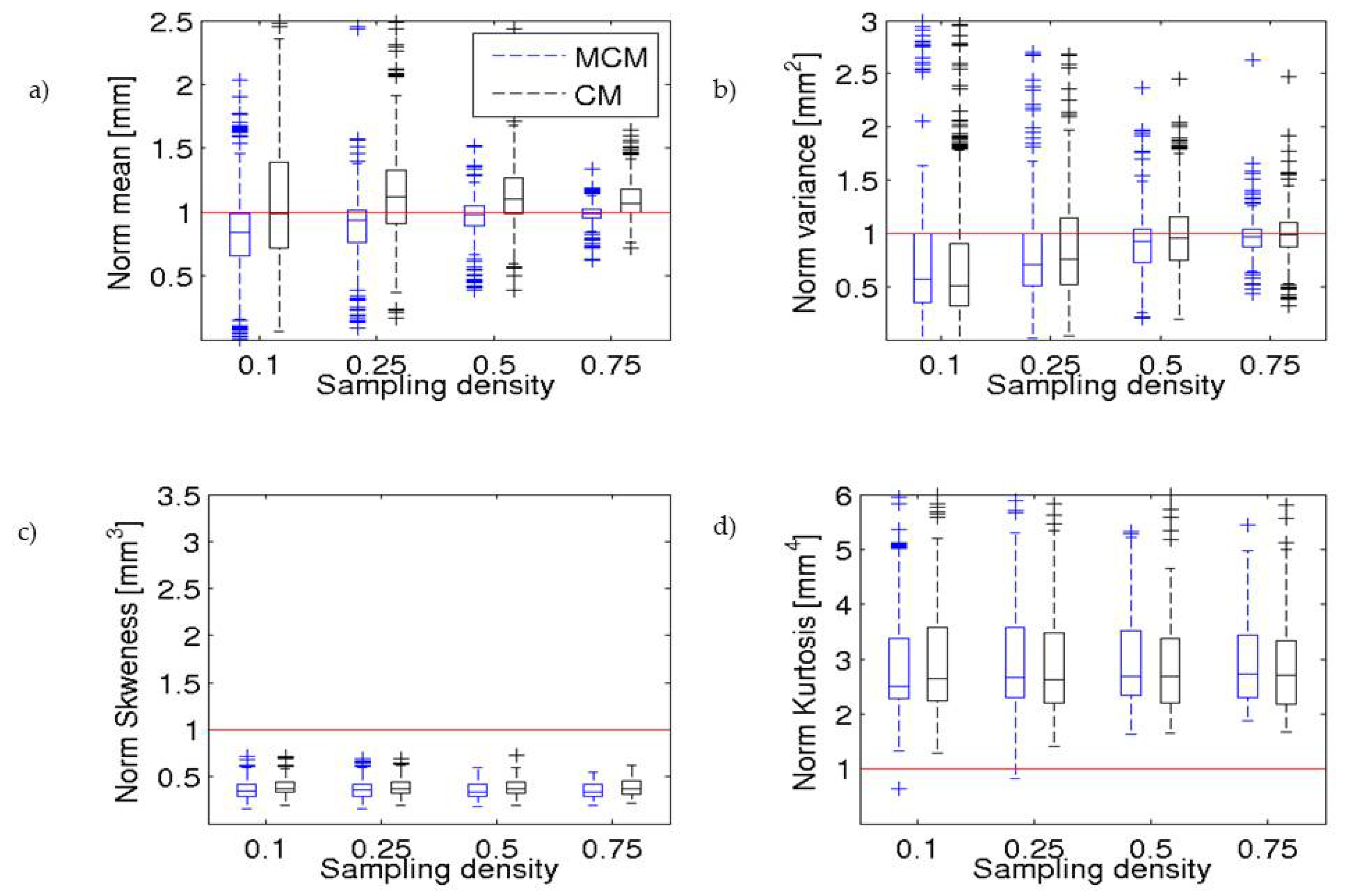
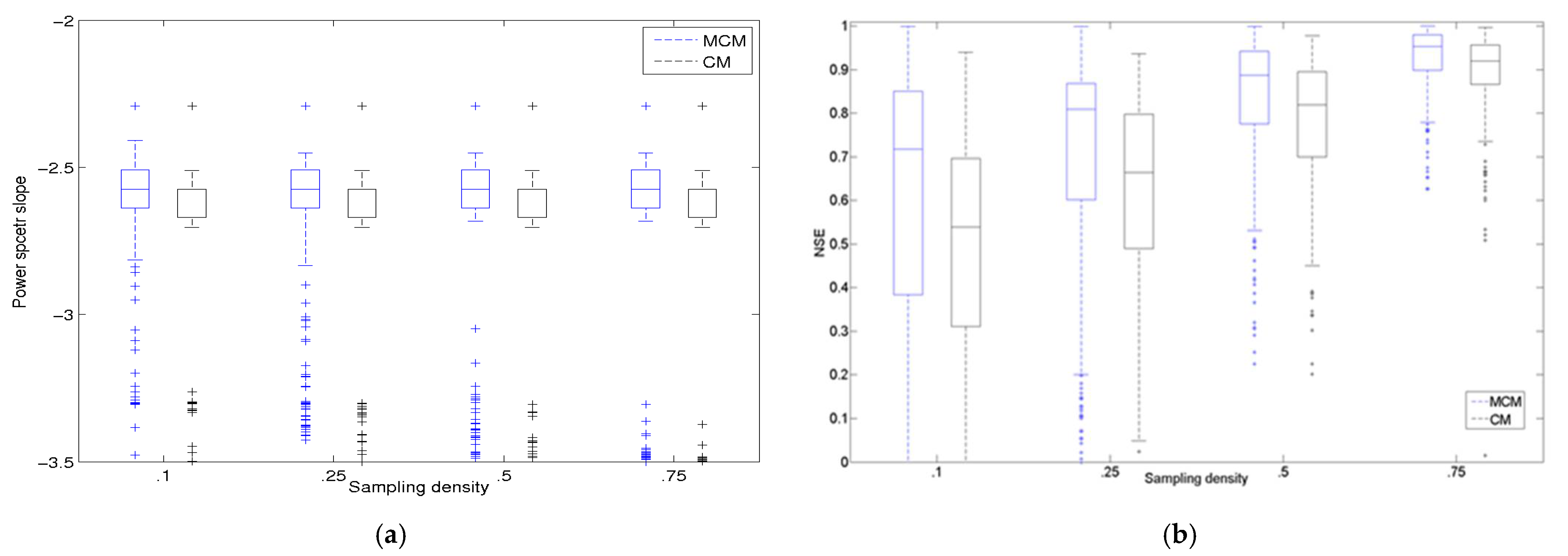
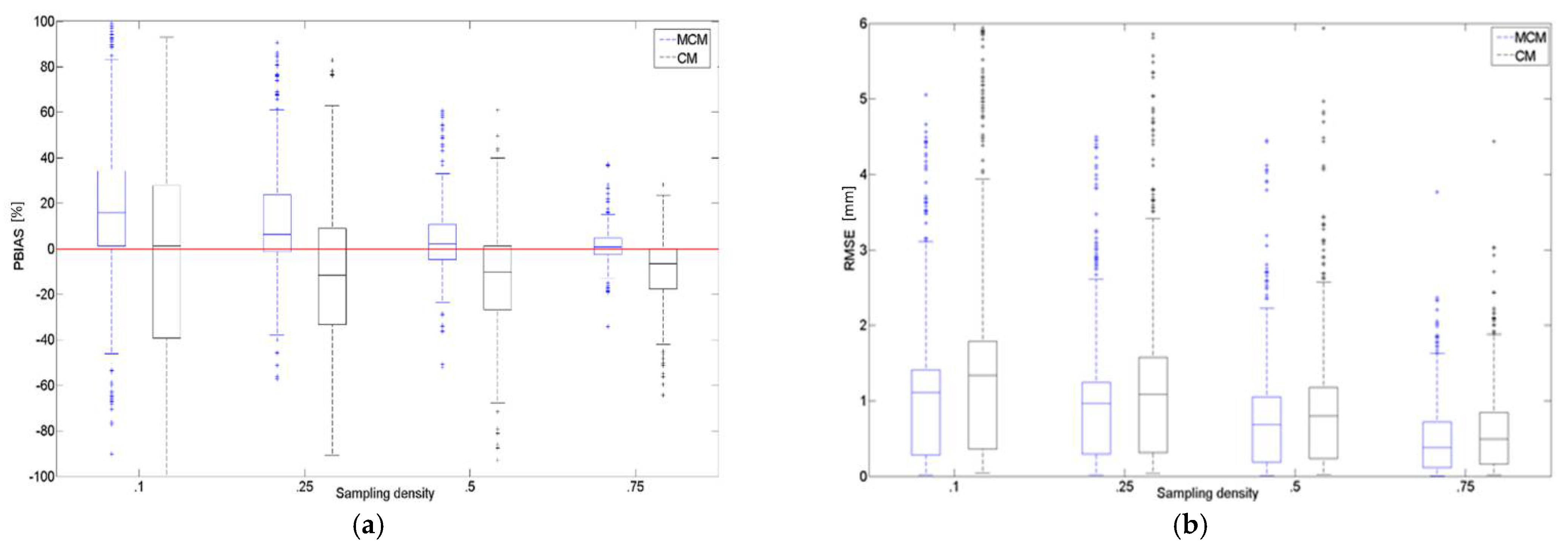
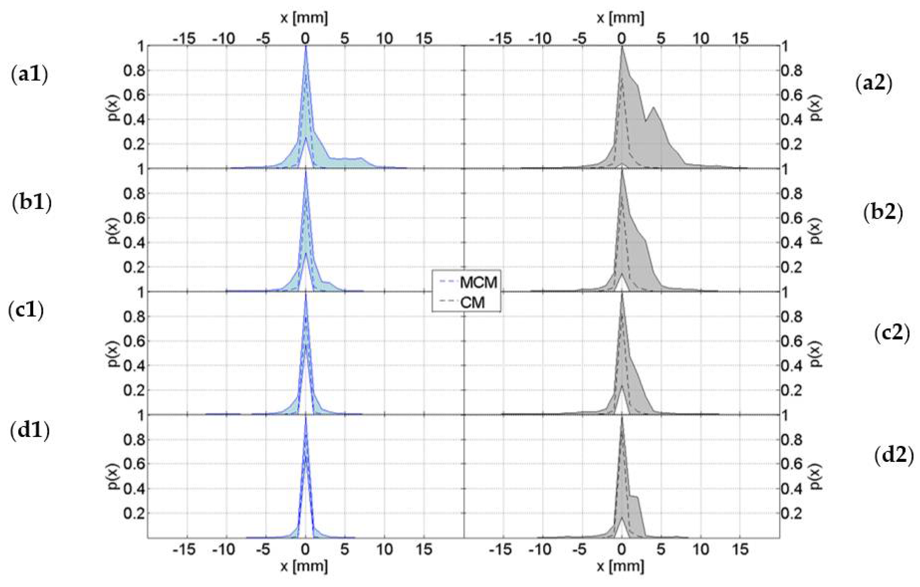
3.1.1. Cross-Validation of MCM

In this section, we report the results of the cross-validation for the 70 selected events, with a graph for each statistic (Figure 6, Figure 7, Figure 8 and Figure 9) in order to point out the differences between the two analysed merging methods (CM and MCM).

The cross-validation was done varying the density of the known measures in order to appreciate how the data-fusion methods can merge the different multi-sources data in any spatio-temporal dataset. The different configurations of MCM (estimate of the local structure per every rain gauge using different formulae and lengths of correlation to fit them) and CM (with equal a priori correlation imposed for every rain gauge) leads to different results, even given the good density of the Italian rain-gauge network. Both methodologies generate maps that preserve the observed values in the location of the observations; the more control points there are, the more similar the maps are. So, the differences between the methods are small especially given the high density of the gauge network and the incremental loss of the surface information used.

CM using kriging and superimposed structure tend to have a smoother and steadier trend with respect to MCM. This behavior leads to an overestimation of the field with respect to MCM. Observing the statistical moments, essentially the mean and the variance, but also the PDF of differences, this behavior is clear and is incremented at low density.

Considering the Power spectra of the different events, the two methods are similar especially considering the event accumulation, while more differences are found considering the smaller scale. The slopes also present very small differences in the values.

One important difference between the two methods is the output coming from the small temporal scale. In fact, the CM spatialize in the same way at small scale as at large scale, not considering the differences in accumulation time. This leads to a substantial overestimation with respect to MCM, especially at small temporal scale.

In every case the quality of results is affected when the study area is spatially very heterogeneous, and the data are affected by errors that cannot be removed even by the filter. If the data locations are dense and uniformly distributed throughout the study area, estimates will be good, regardless of the merging algorithm. In the case of poor density of the measurement network or data affected by all merging algorithms, the highs will be underestimated and the lows will be overestimated.

In conclusion, it is possible to state that the innovations introduced in the MCM, with respect to CM, allow a more accurate estimation of rainfall field at the small spatial and temporal scales, which is particularly important for flash floods.

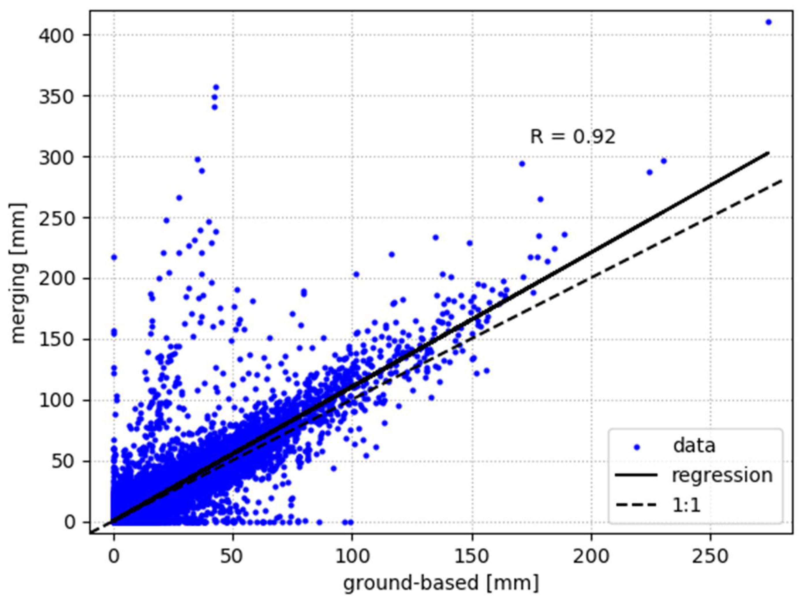
3.1.2. Catchment-Scale Comparison

The two rainfall estimates show a high correlation, with R equal to 0.92 (Figure 10). Furthermore, daily areal mean rainfall from MCM is generally greater than from the ground-based data only (Figure 10). Moreover, daily RMSE varies between 0.8 and 12.4 mm and PBIAS between −60 and 80%, with uniform spatial patterns across Italy and similar behavior between them (Figure 11). It is worth noticing that for most of the study sections, rain gauge and merging rain-gauge–radar QPEs have a closer agreement—RMSE is less than 3 mm for the 58% of the study sections, while the PBIAS is slightly positive and less than the 20% for the 61% of them (Figure 12), evenly distributed all over Italy (Figure 11). A few exceptions show higher RMSE and PBIAS, these latter both positive and negative (Figure 12).

The good agreement between gauge and radar QPE for most Italian catchments confirms the suitability of MCM as input for a hydrological model, not only for civil protection purposes as shown by the event-scale comparison, but also for water resource management and water budget studies. In the following, rainfall fields are further validated at catchment-scale by the performance evaluation of hydrological simulations, in terms of streamflow.

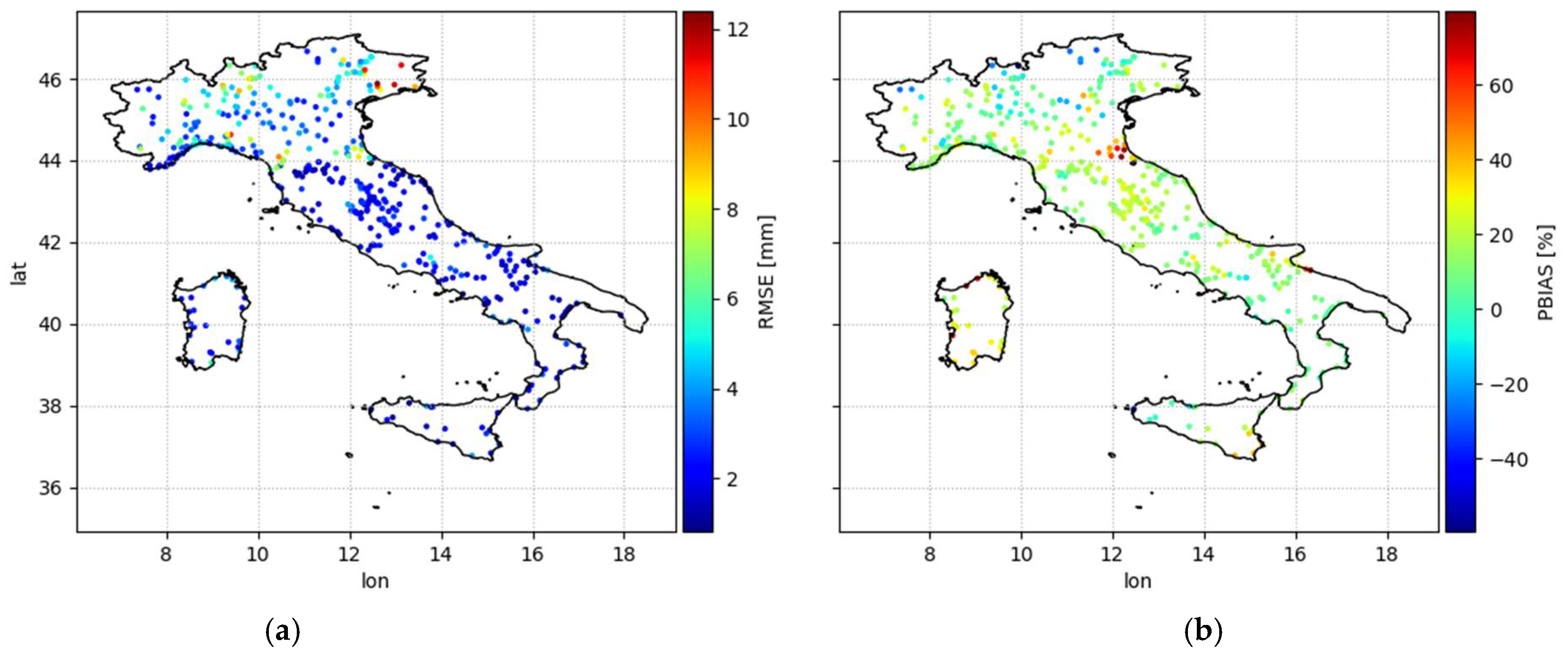
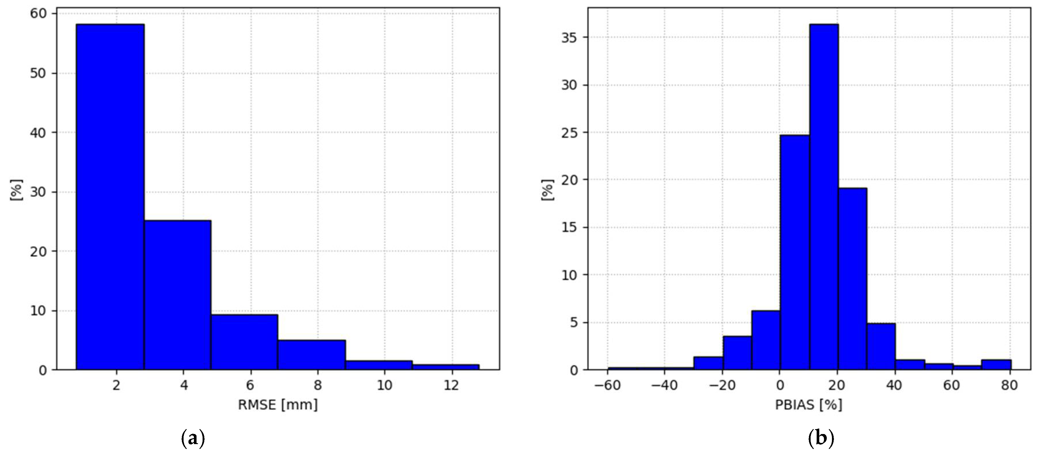
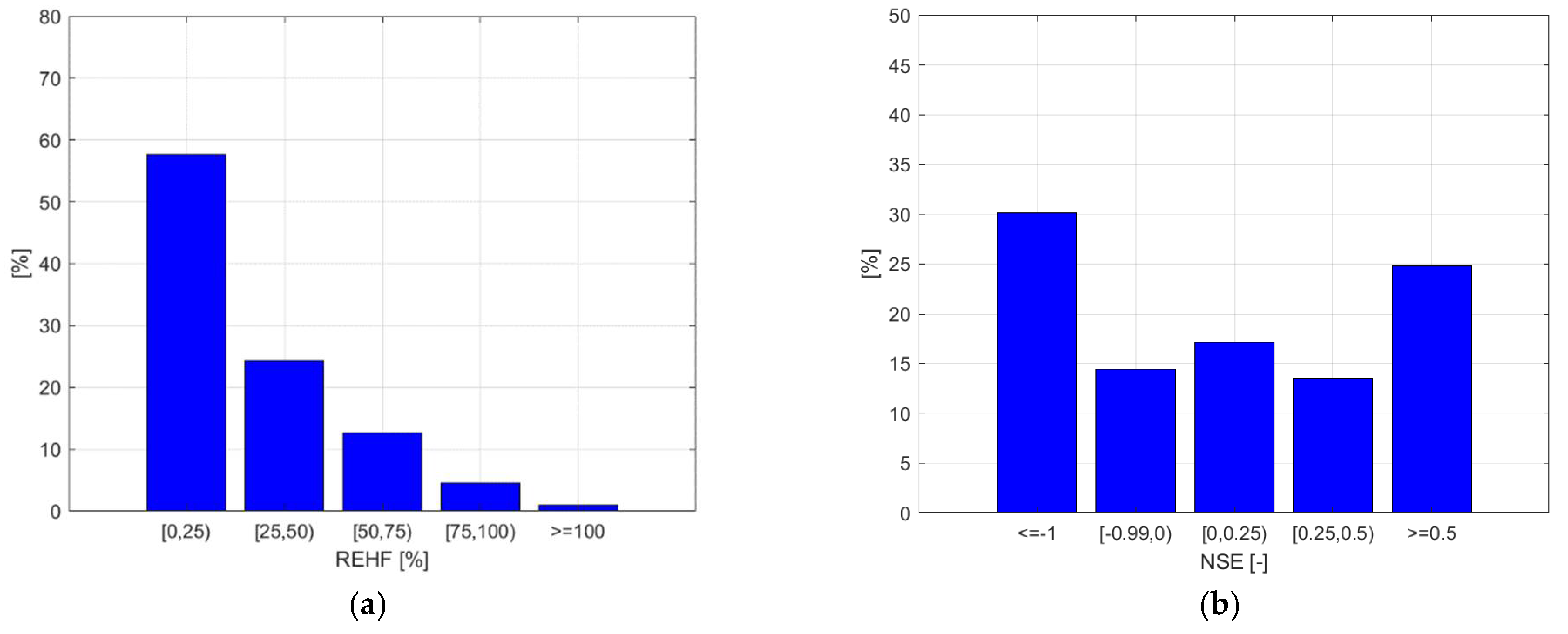
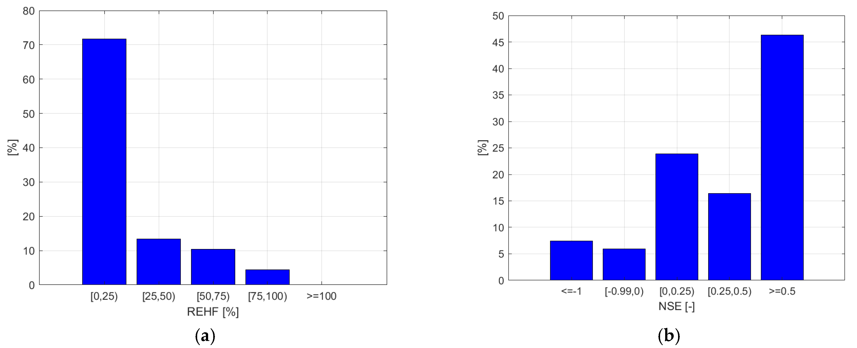
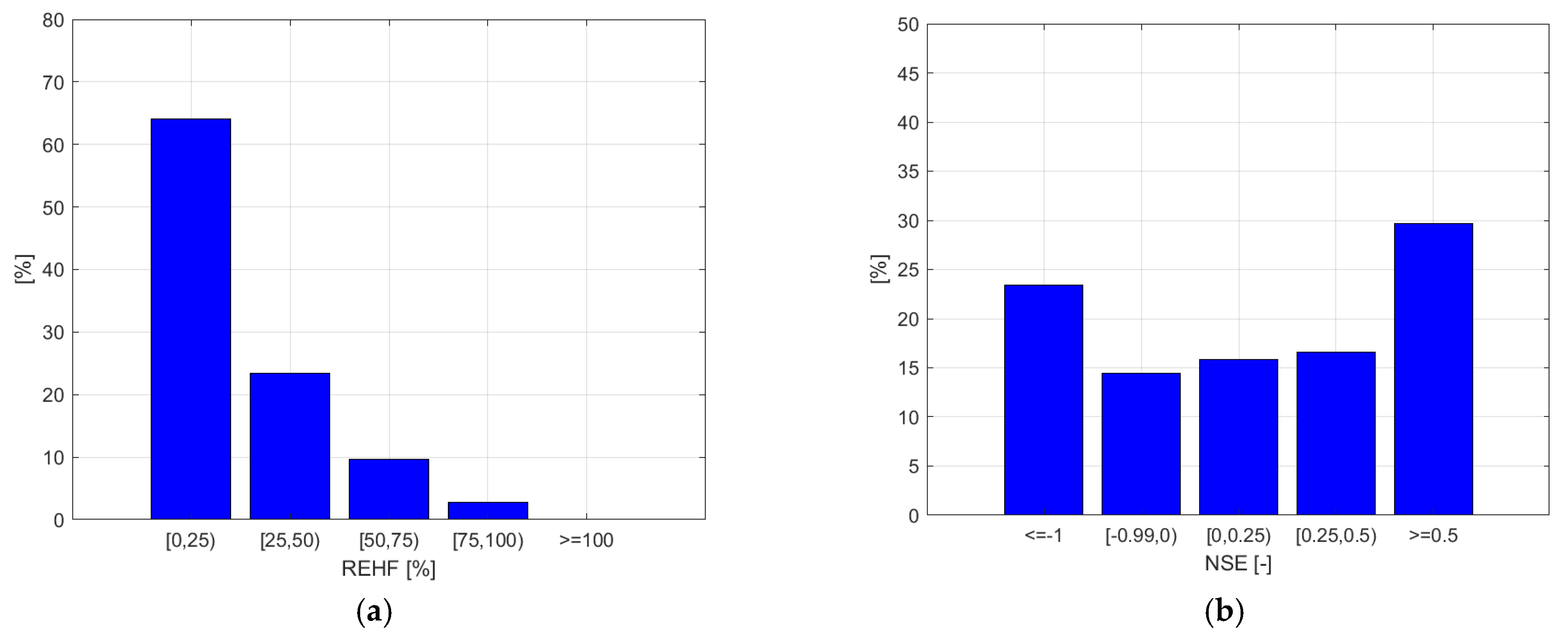
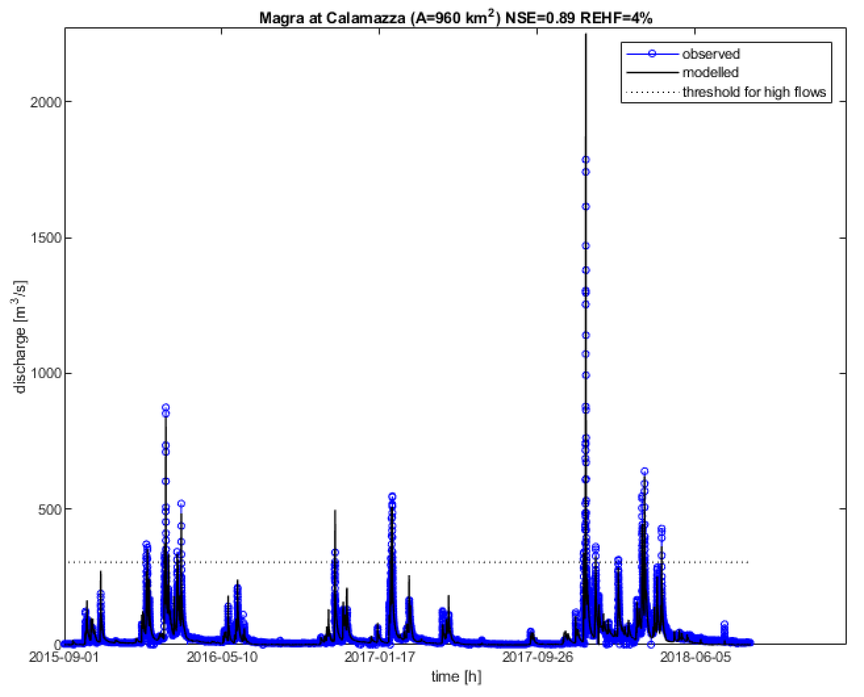
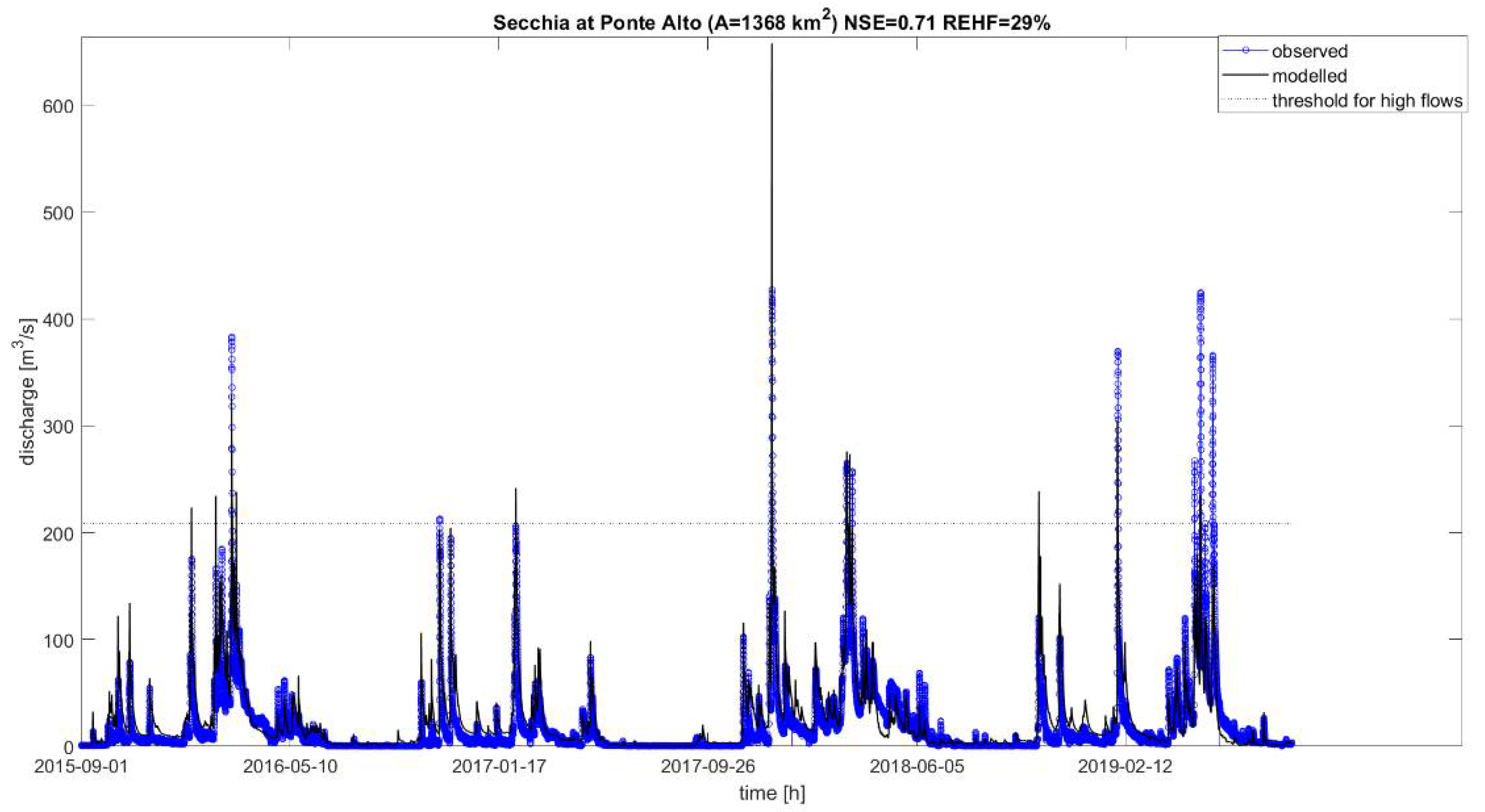
3.2. Performances of Hydrological Simulations

With respect to the performance of hydrological simulations, results are variable, with REHF ranging between 0 and more than 100% in a few exceptions and the NS varying all over its possible range, from negative values up to 1 (Figure 13). Yet, the 58% of the study sections shows a REHF lower than 25%, which is thought to be particularly interesting for a hydrological system specifically designed for high flows monitoring, and 25% of them, a NSE greater than 0.5, which can be set as threshold for satisfactory results [47] (Figure 13). Such results improve considerably if only (i) calibrated sections or (ii) sections with a particularly reliable observed streamflow time series, are considered. In the first case, median REHF is 17% and the 72% of the considered sections has a REHF lower than 25% and the 46% of them a NSE greater than 0.5 (Figure 14), with a median NSE of 0.43. In the second case, the REHF is less than 25% for the 64% of the selected sections and the NSE is greater than 0.5 for the 30% of them (Figure 15). Moreover, results in terms of NSE for calibrated sections are comparable with the ones obtained for example by [28] for a large-scale hydrological reanalysis and they are considered acceptable for a multi-catchment application, although most of the sections do not reach the threshold for satisfactory results (NSE equal to 0.5) according to [47]. Finally, Figure 16 and Figure 17 provide two examples of simulated and observed hydrographs.

4. Conclusions

This work analyzes the performance of a national-scale hydrological monitoring system driven by a multi-sensor based rainfall product. The conditional merging described by [15] was modified in order to exploit radar field information to improve the gauge data interpolation. Then a hydrological model in its operational configuration was used to simulate streamflow and further validate the rainfall algorithm (modified conditional merging, MCM).

Rainfall field analyses evidenced the ability of MCM to provide accurate rainfall estimates at small spatio-temporal scales preserving rain-gauge observations in point measurements but improving the description of rainfall field far from the latter. Moreover, MCM showed good results at catchment-scale (R > 0.9 between daily areal mean rainfall data from MCM and the ground-based product, RMSE < 3 mm/d and PBIAS less than 20% between the two products for most of the study sections (Figure 10, Figure 11 and Figure 12)).

The performance of hydrological simulations is variable. In some cases, skill scores are not very good and this could be related to not-perfect calibration or detail configuration of the model in some specific catchments or even to poorly reliably observed streamflow data used as benchmark. However, in many cases results are satisfactory, with relative error on high flows < 25% and Nash–Sutcliffe efficiency > 0.5 for the 72% and 46% of the calibrated study sections (Figure 14). This confirms the suitability for hydrological monitoring of such an approach, relying on radar and rain-gauge data and a distributed and continuous parsimonious hydrological model. Furthermore, it shows its applicability for operational purposes at a large-scale over a wide range of catchments and climates. Radar data help in capturing those rainfall structures which rarely can be measured even by a dense rain-gauge network, while distributed hydrological models are able to exploit these detailed rainfall fields and opportunely transform them in streamflow by using the runoff formation schematization in a spatial high-resolution framework.

References

1. Shakti, P.C.; Nakatani, T.; Misumi, R. The Role of the Spatial Distribution of Radar Rainfall on Hydrological Modeling for an Urbanized River Basin in Japan. Water 2019, 11, 1703. [Google Scholar] [CrossRef] [Green Version]
2. Tilford, K.A.; Fox, N.I.; Collier, C.G. Application of weather radar data for urban hydrology. Meteorol. Appl. 2002, 9, 95–104. [Google Scholar] [CrossRef] [Green Version]
3. Berenguer, M.; Corral, C.; Sánchez-Diezma, R.; Sempere-Torres, D. Hydrological Validation of a Radar-Based Nowcasting Technique. J. Hydrometeorol. 2005, 6, 532–549. [Google Scholar] [CrossRef] [Green Version]
4. Silvestro, F.; Gabellani, S.; Rudari, R.; Delogu, F.; Laiolo, P.; Boni, G. Uncertainty reduction and parameter estimation of a distributed hydrological model with ground and remote-sensing data. Hydrol. Earth Syst. Sci. 2015, 19, 1727–1751. [Google Scholar] [CrossRef] [Green Version]
5. Corral, C.; Berenguer, M.; Sempere-Torres, D.; Poletti, L.; Silvestro, F.; Rebora, N. Comparison of two early warning systems for regional flash flood hazard forecasting. J. Hydrol. 2019, 572, 603–619. [Google Scholar] [CrossRef] [Green Version]
6. Orellana-Alvear, J.; Celleri, R.; Rollenbeck, R.; Muñoz, P.; Contreras, P.; Bendix, J. Assessment of Native Radar Reflectivity and Radar Rainfall Estimates for Discharge Forecasting in Mountain Catchments with a Random Forest Model. Remote Sens. 2020, 12, 1986. [Google Scholar] [CrossRef]
7. Ochoa-Rodriguez, S.; Wang, L.-P.; Willems, P.; Onof, C. A Review of Radar-Rain Gauge Data Merging Methods and Their Potential for Urban Hydrological Applications. Water Resour. Res. 2019, 55, 6356–6391. [Google Scholar] [CrossRef]
8. Zanchetta, A.D.L.; Coulibaly, P. Recent Advances in Real-Time Pluvial Flash Flood Forecasting. Water 2020, 12, 570. [Google Scholar] [CrossRef] [Green Version]
9. Silvestro, F.; Gabellani, S.; Delogu, F.; Rudari, R.; Boni, G. Exploiting remote sensing land surface temperature in distributed hydrological modelling: The example of the Continuum model. Hydrol. Earth Syst. Sci. 2013, 17, 39–62. [Google Scholar] [CrossRef] [Green Version]
10. Pagano, T.C.; Wood, A.W.; Ramos, M.-H.; Cloke, H.L.; Pappenberger, F.; Clark, M.P.; Cranston, M.; Kavetski, D.; Mathevet, T.; Sorooshian, S.; et al. Challenges of Operational River Forecasting. J. Hydrometeorol. 2014, 15, 1692–1707. [Google Scholar] [CrossRef] [Green Version]
11. Alfieri, L.; Salamon, P.; Pappenberger, F.; Wetterhall, F.; Thielen, J. Operational early warning systems for water-related hazards in Europe. Environ. Sci. Policy 2012, 21, 35–49. [Google Scholar] [CrossRef]
12. Emerton, R.E.; Stephens, E.M.; Pappenberger, F.; Pagano, T.C.; Weerts, A.H.; Wood, A.W.; Salamon, P.; Brown, J.D.; Hjerdt, N.; Donnelly, C.; et al. Continental and global scale flood forecasting systems. Wiley Interdiscip. Rev. Water 2016, 3, 391–418. [Google Scholar] [CrossRef] [Green Version]
13. Pagliara, P.; Corina, A.; Burastero, A.; Campanella, P.; Ferraris, L.; Morando, M.; Rebora, N.; Versace, C. Dewetra, coping with emergencies. In Proceedings of the 8th International Conference on Information Systems for Crisis Response and Management: From Early-Warning Systems to Preparedness and Training, ISCRAM, Lisbon, Portugal, 8–11 May 2011. [Google Scholar]
14. Italian Civil Protection Department. CIMA Research Foundation the Dewetra Platform: A Multi-perspective Architecture for Risk Management during Emergencies. In Business Information Systems; Springer Science and Business Media LLC: Berlin, Germany, 2014; Volume 196, pp. 165–177. [Google Scholar]
15. Sinclair, S.; Pegram, G. Combining radar and rain gauge rainfall estimates using conditional merging. Atmos. Sci. Lett. 2005, 6, 19–22. [Google Scholar] [CrossRef]
16. Parodi, A.; Lagasio, M.; Meroni, A.N.; Pignone, F.; Silvestro, F.; Ferraris, L. A hindcast study of the Piedmont 1994 flood: The CIMA Research Foundation hydro-meteorological forecasting chain. Bull. Atmos. Sci. Technol. 2020, 1, 297–318. [Google Scholar] [CrossRef]
17. Beck, H.E.; Zimmermann, N.E.; McVicar, T.; Vergopolan, N.; Berg, A.; Wood, E.F. Present and future Köppen-Geiger climate classification maps at 1-km resolution. Sci. Data 2018, 5, 180214. [Google Scholar] [CrossRef] [Green Version]
18. Seager, R.; Osborn, T.J.; Kushnir, Y.; Simpson, I.R.; Nakamura, J.; Liu, H. Climate Variability and Change of Mediterranean-Type Climates. J. Clim. 2019, 32, 2887–2915. [Google Scholar] [CrossRef] [Green Version]
19. Blöschl, G.; Hall, J.; Parajka, J.; Perdigão, R.A.P.; Merz, B.; Arheimer, B.; Aronica, G.T.; Bilibashi, A.; Bonacci, O.; Borga, M.; et al. Changing climate shifts timing of European floods. Science 2017, 357, 588–590. [Google Scholar] [CrossRef] [Green Version]
20. Molini, L.; Parodi, A.; Siccardi, F. Dealing with uncertainty: An analysis of the severe weather events over Italy in 2006. Nat. Hazards Earth Syst. Sci. 2009, 9, 1775–1786. [Google Scholar] [CrossRef]
21. Poletti, M.L.; Silvestro, F.; Davolio, S.; Pignone, F.; Rebora, N. Using nowcasting technique and data assimilation in a meteorological model to improve very short range hydrological forecasts. Hydrol. Earth Syst. Sci. 2019, 23, 3823–3841. [Google Scholar] [CrossRef] [Green Version]
22. Avanzi, F.; Ercolani, G.; Gabellani, S.; Cremonese, E.; Pogliotti, P.; Filippa, G.; di Cella, U.M.; Ratto, S.; Stevenin, H.; Cauduro, M.; et al. Learning about precipitation lapse rates from snow course data improves water balance modeling. Hydrol. Earth Syst. Sci. 2021, 25, 2109–2131. [Google Scholar] [CrossRef]
23. Alberoni, P.P.; Ferraris, L.; Marzano, F.S.; Nanni, S.; Pelosini, R.; Siccardi, F. The Italian radar network: Current status and future developments. In Proceedings of the ERAD02, Delft, The Netherlands, 18–22 November 2002; pp. 339–344. [Google Scholar]
24. Vulpiani, G.; Pagliara, P.; Negri, M.; Rossi, L.; Gioia, A.; Giordano, P.; Alberoni, P.; Cremonini, R.; Ferraris, L.; Marzano, F.S. The Italian radar network within the national early-warning system for multi-risks management. In Proceedings of the ERAD08, Helsinki, Finland, 30 June–4 July 2008. [Google Scholar]
25. Marshall, J.S.; Palmer, W.M.K. The distribution of raindrops with size. J. Atmos. Sci. 1984, 5, 165–166. [Google Scholar] [CrossRef]
26. Bancheri, M.; Rigon, R.; Manfreda, S. The GEOframe-NewAge Modelling System Applied in a Data Scarce Environment. Water 2019, 12, 86. [Google Scholar] [CrossRef] [Green Version]
27. Brunner, M.I.; Slater, L.; Tallaksen, L.M.; Clark, M. Challenges in modeling and predicting floods and droughts: A review. Wiley Interdiscip. Rev. Water 2021, e1520. [Google Scholar] [CrossRef]
28. Alfieri, L.; Lorini, V.; Hirpa, F.A.; Harrigan, S.; Zsoter, E.; Prudhomme, C.; Salamon, P. A global streamflow reanalysis for 1980–2018. J. Hydrol. X 2020, 6, 100049. [Google Scholar] [CrossRef] [PubMed]
29. Looper, J.P.; Vieux, B. An assessment of distributed flash flood forecasting accuracy using radar and rain gauge input for a physics-based distributed hydrologic model. J. Hydrol. 2012, 412–413, 114–132. [Google Scholar] [CrossRef]
30. Germann, U.; Berenguer, M.; Sempere-Torres, D.; Zappa, M. REAL-Ensemble radar precipitation estimation for hydrology in a mountainous region. Q. J. R. Meteorol. Soc. 2009, 135, 445–456. [Google Scholar] [CrossRef] [Green Version]
31. Gabella, M.; Joss, J.; Perona, G.; Galli, G. Accuracy of rainfall estimates by two radars in the same Alpine environment using gage adjustment. J. Geophys. Res. Space Phys. 2001, 106, 5139–5150. [Google Scholar] [CrossRef] [Green Version]
32. Todini, E. A Bayesian technique for conditioning radar precipitation estimates to rain-gauge measurements. Hydrol. Earth Syst. Sci. 2001, 5, 187–199. [Google Scholar] [CrossRef] [Green Version]
33. Ebtehaj, A.M.; Lerman, G.; Foufoula-Georgiou, E. Sparse regularization for precipitation downscaling. J. Geophys. Res. Space Phys. 2012, 117, D08107. [Google Scholar] [CrossRef] [Green Version]
34. Xiao, R.; Chandrasekar, V. Development of a neural network based algorithm for rainfall estimation from radar observa-tions. IEEE Trans. Geosci. Remote Sens. 1997, 35, 160–171. [Google Scholar] [CrossRef] [Green Version]
35. Goudenhoofdt, E.; Delobbe, L. Evaluation of radar-gauge merging methods for quantitative precipitation estimates. Hydrol. Earth Syst. Sci. 2009, 13, 195–203. [Google Scholar] [CrossRef] [Green Version]
36. Jewell, S.A.; Gaussiat, N. An assessment of kriging-based rain-gauge–radar merging techniques. Q. J. R. Meteorol. Soc. 2015, 141, 2300–2313. [Google Scholar] [CrossRef]
37. Wilson, J.W.; Brandes, E.A. Radar measurement of rainfall-A summary. Bull. Amer. Meteor. Soc. 1979, 60, 1048–1058. [Google Scholar] [CrossRef] [Green Version]
38. Habib, E.; Krajewski, W.F.; Ciach, G.J. Estimation of Rainfall Interstation Correlation. J. Hydrometeorol. 2001, 2, 621–629. [Google Scholar] [CrossRef]
39. Vulpiani, G.; Montopoli, M.; Passeri, L.D.; Gioia, A.G.; Giordano, P.; Marzano, F.S. On the use of dual-polarized C-band ra-dar for operational rainfall retrieval in mountainous areas. J. Appl. Meteorol. Climatol. 2012, 51, 405–425. [Google Scholar] [CrossRef]
40. Petracca, M.; D’Adderio, L.P.; Porcù, F.; Vulpiani, G.; Sebastianelli, S.; Puca, S. Validation of GPM Dual-Frequency Precipitation Radar (DPR) Rainfall Products over Italy. J. Hydrometeorol. 2018, 19, 907–925. [Google Scholar] [CrossRef]
41. Pignone, F.; Rebora, N.; Silvestro, F.; Castelli, F. GRISO (Generatore Random di Interpolazioni Spaziali da Osservazioni incerte) –Piogge. Rep 2010, 272, 353. [Google Scholar]
42. Nash, J.E.; Sutcliffe, J.V. River flow forecasting through conceptual models part I A discussion of principles. J. Hydrol. 1970, 10, 282–290. [Google Scholar] [CrossRef]
43. Davolio, S.; Silvestro, F.; Gastaldo, T. Impact of Rainfall Assimilation on High-Resolution Hydrometeorological Forecasts over Liguria, Italy. J. Hydrometeorol. 2017, 18, 2659–2680. [Google Scholar] [CrossRef]
44. Silvestro, F.; Parodi, A.; Campo, L.; Ferraris, L. Analysis of the streamflow extremes and long-term water balance in the Liguria region of Italy using a cloud-permitting grid spacing reanalysis dataset. Hydrol. Earth Syst. Sci. 2018, 22, 5403–5426. [Google Scholar] [CrossRef] [Green Version]
45. Madsen, H. Automatic calibration of a conceptual rainfall–runoff model using multiple objectives. J. Hydrol. 2000, 235, 276–288. [Google Scholar] [CrossRef]
46. Alfieri, L.; Pappenberger, F.; Wetterhall, F.; Haiden, T.; Richardson, D.; Salamon, P. Evaluation of ensemble streamflow predictions in Europe. J. Hydrol. 2014, 517, 913–922. [Google Scholar] [CrossRef] [Green Version]
47. Moriasi, D.N.; Arnold, J.G.; Van Liew, M.W.; Bingner, R.L.; Harmel, R.D.; Veith, T.L. Model Evaluation Guidelines for Systematic Quantification of Accuracy in Watershed Simulations. Trans. ASABE 2007, 50, 885–900. [Google Scholar] [CrossRef]
Figure 1. Location of study sections (markers with violet edge are sections with available observed streamflow data).
Atmosphere 12 00771 g001
Figure 2. Italian rain-gauge network (a) and radar network (b). In (b), blue radar icons refer to C-band radars, while light blue ones to X-band radars.
Atmosphere 12 00771 g002
Figure 3. MCM workflow.
Atmosphere 12 00771 g003
Figure 4. Example of empirical 3D local structure evaluated from the radar observation. The values are between 0 (no correlation) and 1 (perfect correlation (located only on the rain-gauge location)).
Atmosphere 12 00771 g004
Figure 5. Difference between MCM (a) and CM (b) regarding the covariance estimation.
Atmosphere 12 00771 g005
Figure 6. Ensemble of statistical moments varying with density. The subplots indicate (a) mean, (b) standard deviation, (c) skewness, and (d) kurtosis.
Atmosphere 12 00771 g006
Figure 7. Ensemble of power spectra slope mean along x directions of the interpolators (a) and NSE (b), varying with the density. The blue lines indicate MCM, while the black ones indicate CM.
Atmosphere 12 00771 g007
Figure 8. Ensemble of PBIAS (a) and RMSE (b), varying with densities. The blue lines indicate MCM, while the black ones indicate CM.
Atmosphere 12 00771 g008
Figure 9. Ensemble of the PDF of differences between run and original field. The subplots correspond to the different sampling percentage of gauge used: (a) 10%, (b) 25%, (c) 50%, and (d) 75%, while the numbers 1 and 2 are the MCM and CM simulations, respectively.
Atmosphere 12 00771 g009
Figure 10. Scatterplot between daily areal mean rainfall from MCM and daily areal mean rainfall from ground-based data.
Atmosphere 12 00771 g010
Figure 11. Maps of RMSE (a) and PBIAS (b) between daily areal mean rainfall from MCM and daily areal mean rainfall from ground-based data.
Atmosphere 12 00771 g011
Figure 12. Frequency histograms of RMSE (a) and PBIAS (b) between daily areal mean rainfall from MCM and daily areal mean rainfall from ground-based data.
Atmosphere 12 00771 g012
Figure 13. Frequency histograms of REHF (a) and Nash–Sutcliffe (b), considering all the study sections.
Atmosphere 12 00771 g013
Figure 14. Frequency histograms of REHF (a) and Nash–Sutcliffe (b), considering only the calibrated sections.
Atmosphere 12 00771 g014
Figure 15. Frequency histograms of REHF (a) and Nash–Sutcliffe (b), considering only the sections which observed discharge, is evaluated with a score greater than or equal to 3.
Atmosphere 12 00771 g015
Figure 16. Comparison between observed and modelled hydrographs for a calibrated section.
Atmosphere 12 00771 g016
Figure 17. Comparison between observed and modelled hydrographs for a section not calibrated but with reliable observed streamflow data.
Atmosphere 12 00771 g017