Article

Subseasonal Forecasts of the Northern Queensland Floods of February 2019: Causes and Forecast Evaluation

Department of Atmospheric Sciences, National Taiwan University, Taipei 10617, Taiwan
*
Author to whom correspondence should be addressed.
Atmosphere 2021, 12(6), 758; https://doi.org/10.3390/atmos12060758
Submission received: 29 April 2021 / Revised: 3 June 2021 / Accepted: 8 June 2021 / Published: 10 June 2021

Abstract

:
During the austral summer 2018/19, devastating floods occurred over northeast Australia that killed approximately 625,000 head of cattle and inundated over 3000 homes in Townsville. In this paper, the disastrous event was identified as a record-breaking subseasonal peak rainfall event (SPRE). The SPRE was mainly induced by an anomalously strong monsoon depression that was modulated by the convective phases of an MJO and an equatorial Rossby (ER) wave. The ER wave originated from an active equatorial deep convection associated with the El Niño warm sea surface temperatures near the dateline over the central Pacific. Based on the S2S Project Database, we analyzed the extended-range forecast skill of the SPRE from two different perspectives, the monsoon depression represented by an 850-hPa wind shear index and the 15-day accumulated precipitation characterized by the percentile rank (PR) and the ratio to the three-month seasonal (DJF) totals. The results of four S2S models of this study suggest that the monsoon depression can maintain the same level of skill as the short-range (3 days) forecast up to 8–10 days. For precipitation parameters, the conclusions are similar to the monsoon depression. For the 2019 northern Queensland SPRE, the model forecast was, in general, worse than the expectation derived from the hindcast analysis. The clear modulation of the ER wave that enhanced the SPRE monsoon depression circulation and precipitation is suspected as the main cause for the lower forecast skill. The analysis procedure proposed in this study can be applied to analyze the SPREs and their associated large-scale drivers in other regions.

1. Introduction

In late January and early February 2019, Queensland was hit by a disastrous rainfall event that caused 18,000 residents to lose power and hundreds of others to evacuate. The floods led to huge losses for farmers, and estimates of 625,000 head of cattle and 48,000 sheep were killed [1,2,3].
The annual rainfall in Australia shows a relatively high rainfall amount along the northern and eastern coastline. The northern part of Australia receives more than 50% of the rainfall amount of the annual totals in summer, where the water vapor is primarily brought by the Australian summer monsoon [4]. The Australian summer monsoonal region is generally regarded as 115°~150° E, 5°~20° S in many studies [5,6,7]. The subseasonal variability of monsoonal flow and rainfall are affected by multiple-scale phenomena, such as Madden–Julian oscillation (MJO) [8,9,10], convectively coupled equatorial waves (CCEWs) [11,12], tropical cyclones (TCs) [13,14], and/or extratropical surges [6]. King et al. [15] pointed out that the extreme rainfall variability is closely related to the mean rainfall variability during austral summer, especially the TCs and east coast low (monsoon depression). They defined the extreme rainfall as the monthly maximum consecutive 5-day precipitation totals. On the other hand, in order to evaluate the usefulness of subseasonal to seasonal (S2S) prediction [16], Tsai et al. [17] defined a subseasonal peak rainfall event (SPRE) as the maximum successive three-pentad (15-day) precipitation within a three-month time window. The SPRE is an ideal target for assessing the baseline prediction skill of a S2S prediction model before applying model products to local usages [18]. The SPRE by definition is the most significant 2-week rainfall episode in the monthly time scale. Therefore, it is deemed to be the most important S2S precipitation prediction target.
Cowan et al. [1] gave a thorough analysis of the large-scale climate conditions of the 2019 Queensland flood. They found this event was a good example to promote the awareness of the benefit of S2S prediction that showed good skill in forecasting the broad-scale atmospheric conditions north of Australia a week ahead. Motivated by Cowan et al. [1], the purpose of the present paper is twofold. First, it provides additional evidence showing that the 2019 Queensland floods are associated with an SPRE influenced by multiple large-scale factors. Secondly, it designs some informative targets that reflect some essential characteristics of the SPRE and can be used in model prediction verification and comparison. To leverage the dynamic model prediction data from the S2S Project Database [19], the forecast targets will include the influential circulation patterns and subseasonal scale accumulated precipitation.
The paper is organized as follows: Section 2 describes the observational and S2S datasets we use. Section 3 documents the 2019 northern Queensland event and its relationship with monsoon depression, MJO, and CCEWs. Section 4 discusses the prediction performance of S2S models for the 2019 event. The prediction skill is also accessed based on the hindcast data from 1998 to 2018. Section 5 is a summary of findings and discussions.

2. Data and Methods

2.1. Data

The wind field is based on the European Centre for Medium-Range Weather Forecasts Reanalysis Interim (ERA-Interim) [20], which is utilized with a horizontal resolution of 0.75° × 0.75° in longitude and latitude during the period from November 1998 to February 2019. Rainfall data are based on the CPC MORPHing technique (CMORPH) precipitation data with a spatial resolution of 0.25° × 0.25°. It includes the raw, satellite only precipitation estimates, corrected, and gauge-satellite blended precipitation products, with calibration against surface gauge observations [21]. Outgoing longwave radiation (OLR) is used as an appropriate proxy for the deep convection, which is based on the interpolated daily OLR version 1.2 from National Oceanic and Atmospheric Administration (NOAA) Climate Data Record (CDR) with the spatial resolution of 1° × 1° [22].
The forecast data are downloaded from the S2S Project Database [19]. Both hindcast and forecast data contributed by 11 forecast centers around the world (Table 1) are available in the database. Total precipitation and wind field are used in this study. In this study, we need to collect the model output with initialization frequency at least once every 5 days. However, at the time when the research was carried out in 2020, only four out of the eleven models, namely the BoM, CMA, ECMWF, and NCEP, provided both hindcast and forecast datasets that satisfy this criterion. Therefore, these four models are presented in this paper for model prediction, verification, and comparison. We have also checked the forecasts produced by JMA, KMA, and UKMO, but the results were not presented due to the sampling limitation.

2.2. Identifying MJO and CCEWs

We utilize the space-time filtering technique developed by Wheeler and Kiladis [23] to identify MJO and CCEWs. The first step is to remove the seasonal cycle by subtracting the long-term mean and the first three harmonics of the daily climatology based on the 1979–2018 period for each grid. To retain the full signal of the waves [24], the anomalies of the symmetric and antisymmetric components of the waves are not decomposed. Then, the Fourier transform in longitude is performed, followed by another transform in time. Fourier coefficients outside the range of the filter are then set to zero, and the filtered data are obtained by performing the inverse transform. The spectral bands used in the space-time filter technique for CCEWs are based on the dispersion relation
ω 2 k 2 k ω = 2 m + 1        m = 1 ,   2 ,  
The wavenumber (k), frequency bands (ω), and equivalent depths (h) for equatorial Rossby wave and MJO are presented in Table 2. The influences of other tropical modes are less significant (figure not shown). Note that the wavenumber of MJO is positive, which means that the wave propagates eastward, and the other is negative. This calculation is provided by Carl Schreck, III (SUNY at Albany, see https://ncics.org/portfolio/monitor/mjo/, last accessed, 9 June 2021), and the function can be applied to the NCAR Command Language (NCL) (see https://www.ncl.ucar.edu/Document/Functions/User_contributed/kf_filter.shtml, last accessed, 9 June 2021).
The convection modulation of MJO and individual CCEWs is identified based on the same procedure described in Tsai et al. [17]. We use the rank order of the wave-filtered OLR to flag the dates of the study period as a day of the “convective”, “no signal”, and “suppressed” phases. The convective status of each wave is determined according to the threshold values of the wave-filtered OLR. The threshold values are defined by the first ( Q 25 ) and third ( Q 75 ) quartiles of the filtered daily OLR anomalies collected during the boreal winter half year (November-April) from 1998 to 2015 of all grid points in a large domain bounded by the longitudes of 105° E and 135° E and latitudes of 15° S and 15° N. The thresholds for each type of wave are summarized in Table 1 of Tsai et al. [17]. When the filtered OLR anomaly is lower than Q 25 and the raw OLR value is less than 250 W m−2, the day is flagged as the convective phase, while if it is higher than Q 75 , the day is flagged as the suppressed phase, otherwise the day is flagged as no signal. For MJO (ER), the Q 25 and Q 75 values are −8.84 W m−2 (−7.48 W m−2) and 8.69 W m−2 (7.33 W m−2), respectively.

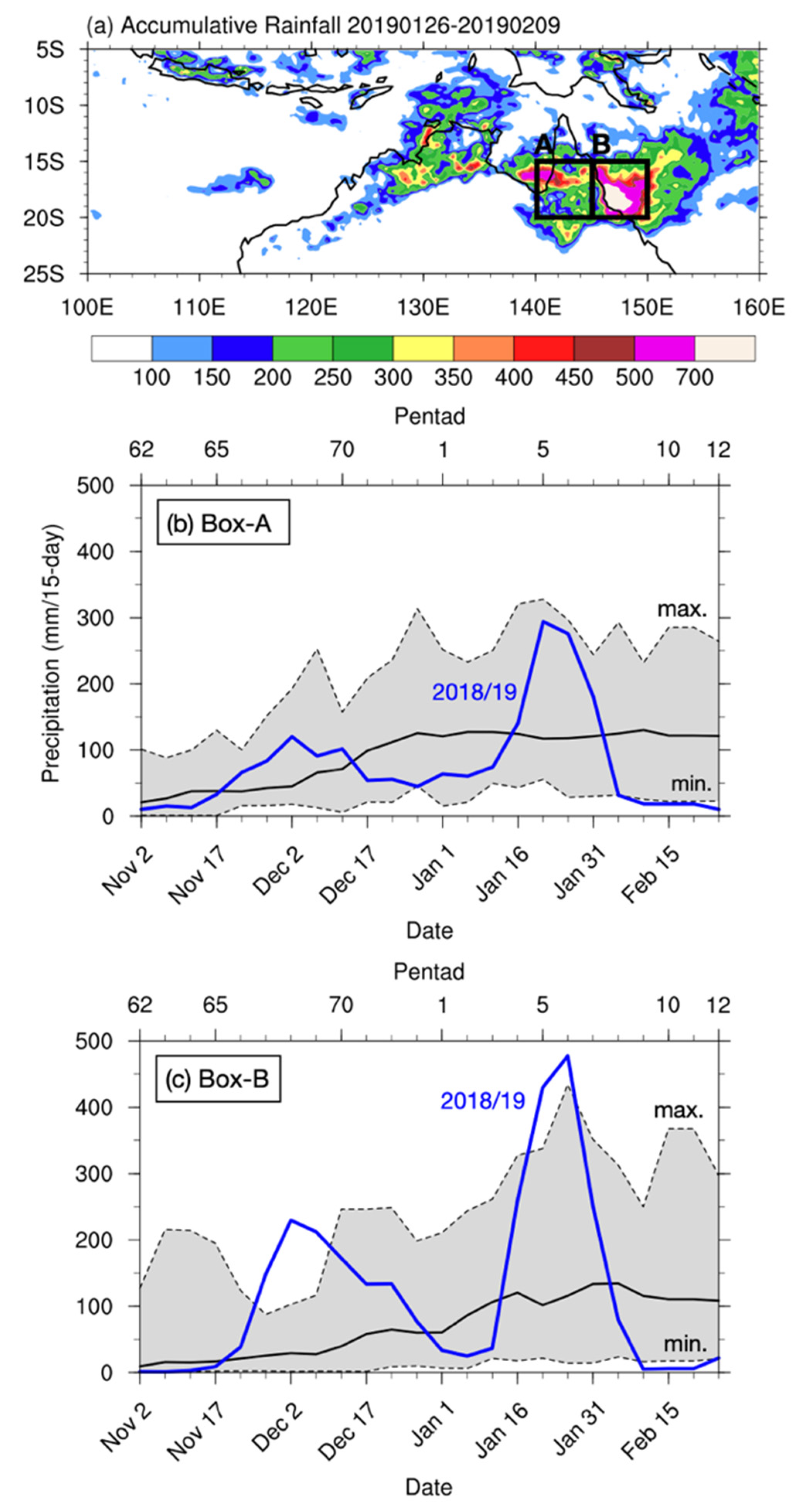
3. The 2018/19 Northern Queensland SPRE

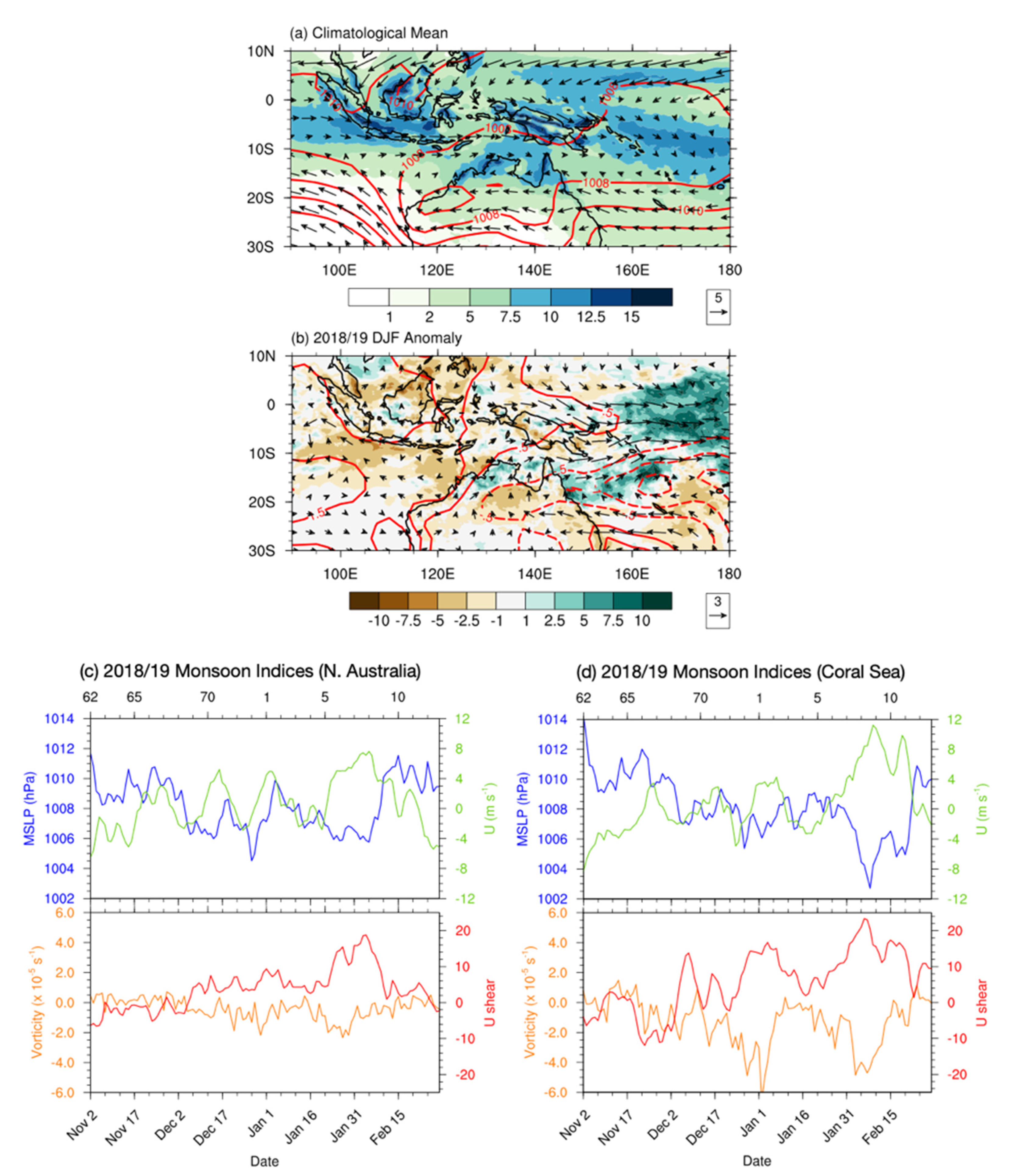
3.1. Australia Monsoon Trough

In this subsection, we will discuss the northern Queensland SPRE during the 2018/19 austral summer (December to February) represented by two box areas marked in Figure 1a. The SPRE is identified based on the CMORPH dataset. The time series of the area mean 15-day accumulative precipitation running by pentad from November 2018 to February 2019 is presented in Figure 1b,c. In both areas, the maximum 15-day accumulated rainfall occurred during the successive pentads from P5 to P8 (21 January–9 February). The beginning time of the Box-A SPRE is one pentad earlier than that of the Box-B SPRE. In order to see how extreme the 2018/19 case is compared with the climatological rains, the twenty years (1998–2017) of minimum and maximum 15-day accumulative precipitation are plotted together with the 2018/19 rainfall amount in Figure 1b,c. The gray shaded area in Figure 1b,c marks the range between maximum and minimum 15-day rainfall amount running by pentad. It is evident that the precipitation over the east coast (Box-B) is more abundant than the inland region (Box-A). For Box-A the transition time from dry to wet is around mid-December (P70). For Box-B the transition time appears in two stages with the first in mid-December, which is the same as that of Box-A, and the second in mid-January (P3), where the Box-A shows a similar level of rainfall as in late December without showing any sharp increase. Compared with the historical data, it is clear that the 2018/19 SPRE at Box-B broke the twenty-year pentad rainfall record. It is interesting to see the oscillations on the subseasonal time scale in both areas. In the following, we will discuss the relationship between the subseasonal variations of precipitation and the monsoon trough, MJO, and CCEWs.
The relationship between the monsoon trough and major precipitation areas can be illustrated using the 20-year climatological mean seasonal (DJF) precipitation, sea level pressure (SLP) and 850-hPa wind (Figure 2a). Figure 2a sees Australia covered by a large and elongated low-pressure center characterized by a cyclonic circulation in a clockwise direction. It extends northeastward to the east of New Guinea. The precipitation regions in general correspond to the region with cyclonic flow (negative relative vorticity in southern hemisphere), but the rainfall amount is stronger along the coast, and it decreases southward. The monsoon trough over northern Australia is formed with a strong zonal wind shear that has the westerlies in the north and the easterlies in the south. The westerlies flow from the Indian Ocean through the Timor Sea and the Arafura Sea to the Pacific Ocean, and the easterlies flow from the Pacific Ocean through northern Australia to the Indian Ocean. On the other hand, on the equatorial Pacific side, the monsoon trough straddles the equator with the easterlies to the north of the equator and westerlies blowing from Indonesia and the New Genia islands. The 2018/19 austral summer monsoon trough anomalies presented in Figure 2b clearly show a deepened trough especially in northwestern Australia, with an anomalous low-pressure system and cyclonic flow extended to the Coral Sea and the Western Pacific. The enhanced monsoon low also brings strong westerlies in the north and easterlies in the south. However, the positive rainfall anomaly is confined only along the northern coast of Australia and the Coral Sea; over land area, the rainfall is mainly less than the climatological means.
The summer monsoon and monsoon depression can be described using the indices such as the area mean SLP, 850-hPa zonal wind and vorticity over the monsoon region (115°~145° E, 5°~20° S) and the Coral Sea (145°~165° E, 5°~20° S), and 850-hPa zonal wind shear (U850[5°–15° S, 115°–145° E]–U850[20°–30° S, 115°–145° E] and U850[5°–15° S, 145°–165° E]–U850[20°–30° S, 145°–165° E], respectively) to quantify the summer monsoon and monsoon depression intensity and variability. This index is a modification of the AUSSM index proposed in Yim et al. [25] based on the climatological monsoon depression in Figure 2a, where the westerlies appear in the north and easterlies in the south. After comparing the difference between the wind shear and the westerly [6,7,26] monsoon indices, we found that the wind shear index has the merit of showing clear seasonal contrast separated by the onset date and the cyclonic structure of the clockwise (cyclonic) monsoon depression over the interior of northern Australia [27]. The subseasonal variations of these indices in summer 2018/19 can be easily identified in Figure 2c,d. A strong westerly surge occurred in late January and lasted until mid-February. Associated with this westerly surge we see strong westerly wind shear. The westerly wind shear sharply dropped during the second week of February, together with a sharp increase in SLP and the anticyclonic vorticity. Comparing Figure 1c and Figure 2c, it is evident that the large-scale monsoonal environment of the SPRE can be characterized by rapid intensification of the low-level westerly flow, the enhanced westerly wind shear and cyclonic circulation, and low surface pressure. The subseasonal enhancement of the monsoon trough over northern Australia created a favorable condition for the precipitation to persist. This is consistent with the findings in Cowan et al. [1].
The subseasonal relationship between the large-scale environment and northern Queensland rains can be clearly seen in the pentad maps from mid-January to mid-February. Figure 3 shows the pentad-mean 850-hPa wind field and precipitation maps from 16 January to 14 February. In two pentads before the SPRE (Figure 3a,b), Queensland received easterlies, implying that the monsoon trough was weak during this period. From 26 January, the monsoonal westerly started to intensify (Figure 3c), and a cyclone formed over the Arafura Sea and northeastern Queensland. The monsoon depression subsequently moved southward and strengthened, which brought abundant rainfall into the continental part of northeastern Queensland. During the peak pentad of the SPRE episode, the center of the monsoon depression was right over northeastern Queensland (Figure 3d), which enhanced the moist westerlies along the north coast and the moist northeasterlies over the Coral Sea that brought the moist air to the east coast of Queensland. This slow-moving monsoon depression appears to be the culprit for the disastrous rainfall event.

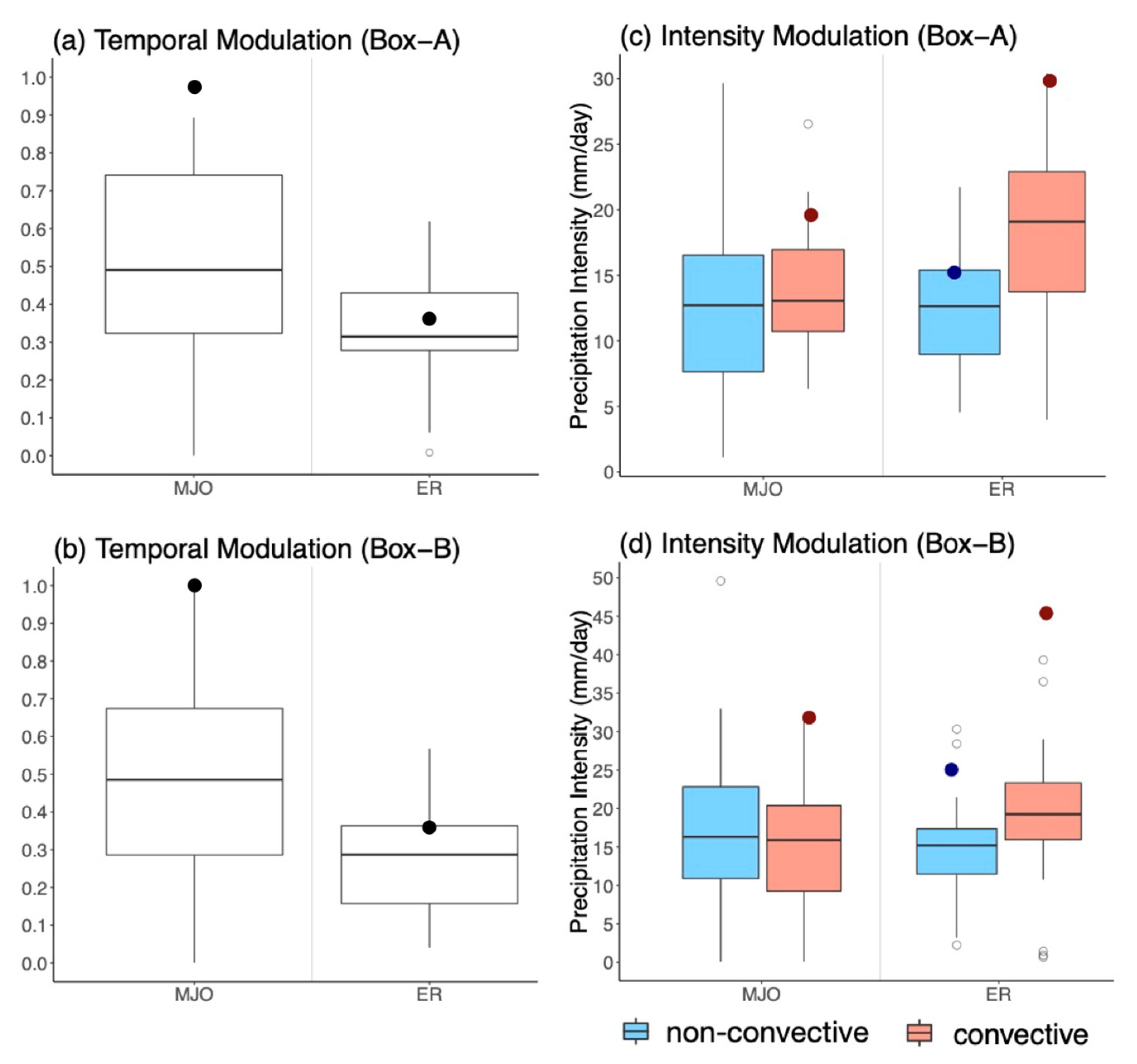
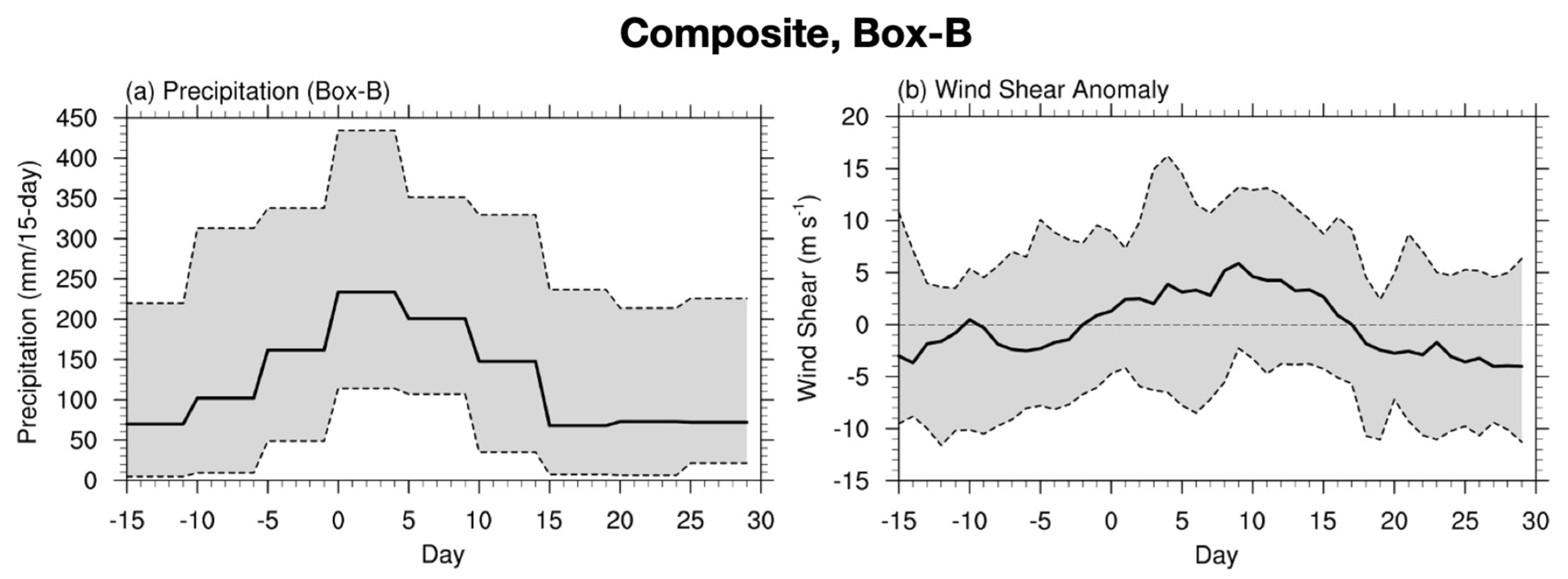
3.2. MJO and Equatorial Rossby Wave

Convection activity over northern Australia is frequently influenced by MJO and CCEWs [28]. The MJO circulation pattern reveals a Kelvin–Rossby couplet structure [29], which usually enhances the monsoon depression and leads to rainfall perturbations, especially in phases 5 to 7 [30]. During the occurrence period (26 January–9 February) of the 2018/19 Box-B SPRE, Figure 4a shows that a strong MJO convective phase passed through northern Australia. The MJO phase diagram (Figure 4b) indicates that the MJO remained strong during January and February. At the same time, a westward-propagating ER wave arrived from the South Pacific. Figure 4a shows when the ER moved into the convective zone of MJO in late January, it clearly enhanced the precipitation. Heavy precipitation persisted for more than two weeks before the rain band moved eastward to the South Pacific with the MJO. Note that the westward-propagating ER waves from the Pacific to the Indian Ocean originated from the active deep convection over the tropical central Pacific. The enhanced convection can be identified in Figure 2 as the large area of positive precipitation anomalies over the tropical Pacific to the east of Papua New Guinea. The tropical Pacific during the 2018/19 austral summer was characterized by a transition from a diminishing La Niña in 2018 to the development of a weak El Niño by early 2019 [31]. The central Pacific in the tropics over both northern and southern hemispheres was warmer than normal during January 2019, which enhanced the convection and precipitation near the dateline (160°–180° E).
The general relationship between the northern Queensland SPREs and the MJOs and ERs is checked based on the frequency that the SPREs and the convective phases of MJO and ER occurred concurrently. The results listed in Table 3 show that for the SPREs in 21 austral summers (DJF) from 1998/99–2018/19, all Box-B SPREs occurred when either the MJO or the ER convective phase passed through, with 57% of the SPREs that occurred when both MJO and ER were in convective phases The years with the largest three SPRE rainfall amounts (2018, 2008, 2006) all occurred concurrently with the convective phases of MJO and ER. Box-A has a higher percentage (76%) of the SPREs that occurred concurrently with the convective phases of MJO and ER than Box-B. However, the Box-B SPRE contributed a higher percentage of the rainfall to the seasonal (DJF) totals compared with the Box-A SPREs. Table 3 shows that for Box-A, the medium of the ratio of an SPRE event to the DJF totals is 31.8%, while for Box-B, the medium is 44.4%. For Box-A, only one year (2018) shows a ratio higher than 50%, while for Box-B seven years show higher than 50% ratios. This suggests that the North Queensland east coast is more sensitive to subseasonal variability. Nevertheless, it is evident in Table 3 that the 2018/19 SPRE is remarkable because for Box-A, the event contributed the largest (50.9%) portion to the seasonal rainfall totals, and for Box-B, the event’s total accumulated rainfall amount (477.4 mm) was the largest in 21 years.
To further quantify the MJO and ER modulation on the SPRE rainfall, we calculated the percentage of the time during the 15 days of SPREs that the waves are in convective phases. We use this time percentage as a measure of the temporal modulation of MJO and ER on the SPRE rainfall. We also calculated the ratio of mean rainfall intensity during the convective phase against the mean rainfall intensity during the nonconvective condition (no-signal and suppressed phases) and used the ratio as a measure of intensity modulation of the waves. The results shown in Figure 5 suggest an abnormally strong modulation of MJO and ER on the 2018/19 SPREs over both Box-A and Box-B areas. During the 2018/19 Box-A SPRE, almost all of the 15 days of OLR were in the MJO convective phase, of which the percentage is much higher than the SPRE during other years. The convective phase of ER waves is about 35% which is also above the medium percentage of the 20 years from 1998–2017. On the other hand, Figure 5b shows that during all of the 15 days of the Box-B SPRE the OLR was in convective phase, which is the highest compared with the past 20 years. The percentage of the convective phase of ER also reaches the upper quartile in 20 years, which is clearly above the medium. Therefore, we can conclude that in the 2018/19 case, the temporal modulation of both MJO and ER on the northeastern Queensland SPREs was the strongest since 1998. Regarding the rainfall intensity modulation, we can see in Figure 5c,d that climatologically the rainfall intensity in Box-A is almost two times stronger during the ER convective phase compared with the nonconvective phase, while the difference is smaller in Box-B. On average, the rainfall intensity in two box areas is similar during the ER convective phases, but the variability in Box-A is larger. During the ER nonconvective days, the rainfall intensity in Box-B is slightly larger than that in Box-A. The SPREs in the 2018/19 summer are unusual. Note that the rainfall intensity in Box-B is much larger than in Box-A, although in both areas the intensity is strongest since 1998. The ER modulation is particularly strong. The average rainfall intensity during the ER convective days is almost twice the intensity of the nonconvective ER days.

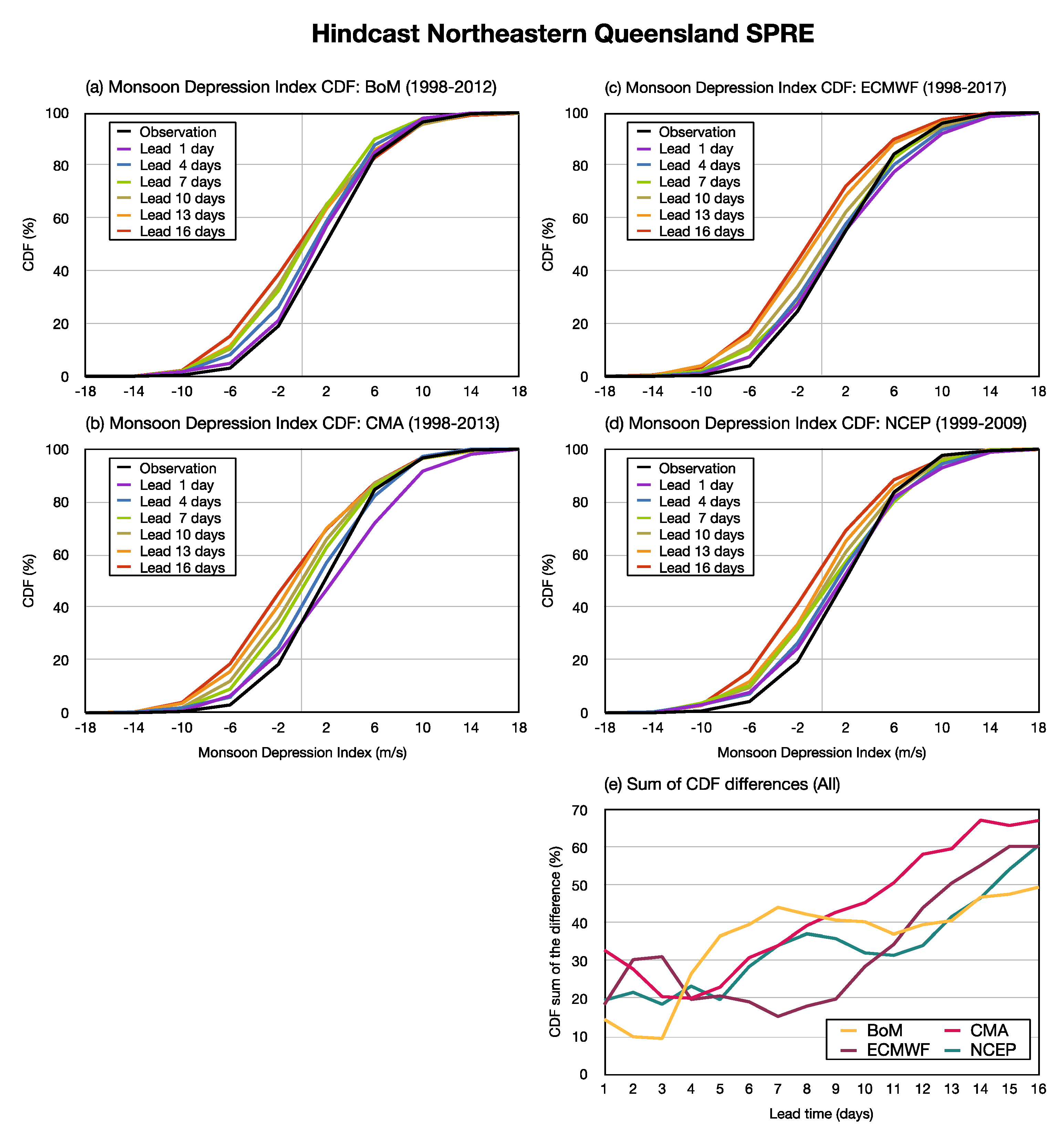
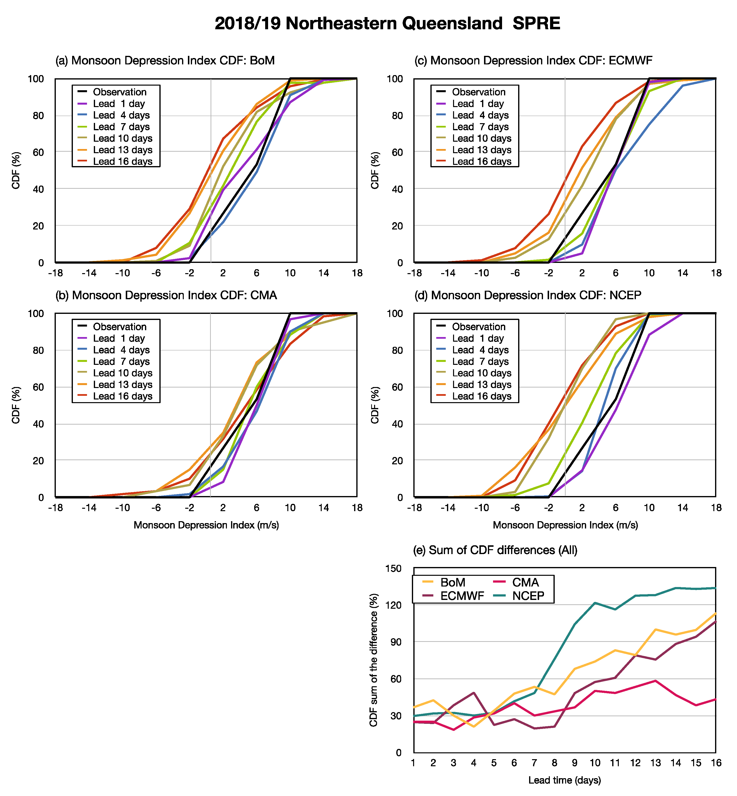
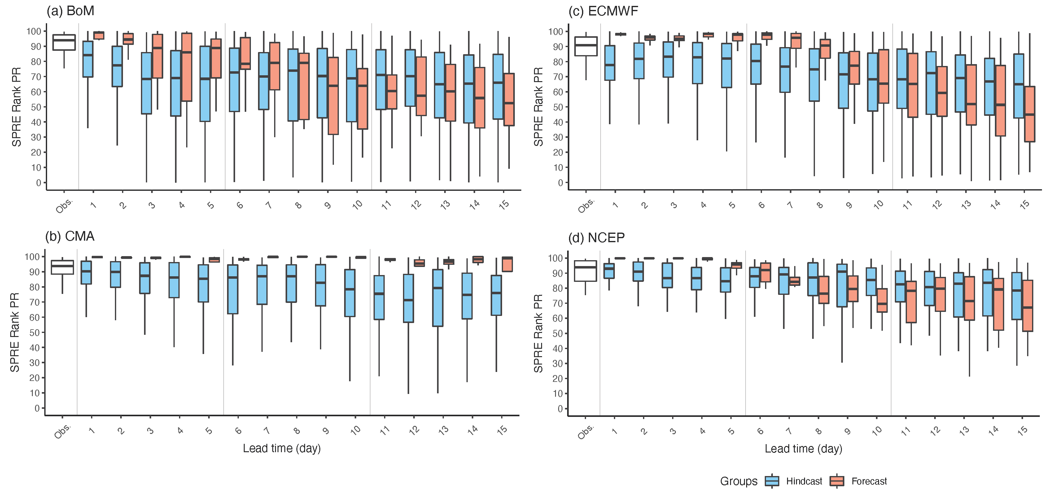
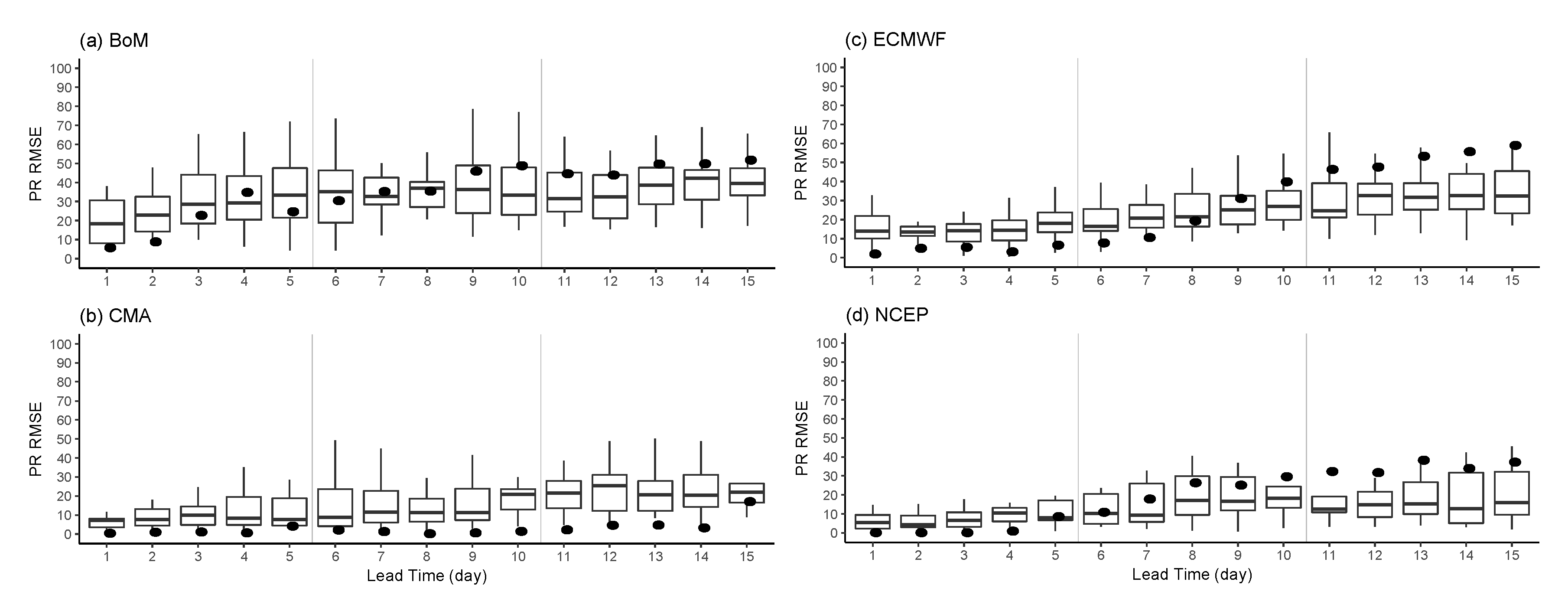
4. S2S Prediction Evaluation

After seeing the close relationship between monsoon depression and the SPREs, in this section, we will present the assessment of the extended-range forecast quality of the SPREs based on the S2S database. The analysis strategy is, first, to evaluate whether the forecast data can capture the monsoon depression index variability within a 45-day window measured by the zonal wind shear index. Second, we evaluate the rainfall forecast skill with a calibration concept so that all model products can be compared and understood. Two approaches are exercised in this study. One is the percentile rank (PR) of the SPRE rainfall amount based on the percentage distribution of the running 15-day accumulated total rainfall during a season (DJF) obtained from the hindcast database of each model. Another is the percentage contribution of the SPRE rainfall amount to the three-month seasonal (DJF) totals. For the forecast ratio (percentage contribution), the calculation is based on the hindcast database of each model. As the accumulated rain and variability in Box-B is larger than that in Box-A (Figure 1), and the 2018/19 flood is more extreme in Box-B, particularly in Townsville, we will focus on the Box-B SPREs. In the rest of the paper, Box-B is used interchangeably for northern Queensland.

4.1. Monsoon Depression Index Variability

Figure 6a shows a composite 45-day time series with the three SPRE pentads from Day(0) to Day(14), the three pentads before the SPREs from Day(-15) to Day(-1), and the three pentads after the SPREs from Day(15) to Day(29). The black curve is the average of the 20-year (1998–2017) 15-day accumulative rainfall running by pentad, and the gray shade shows the range of the 15-day rainfall for each pentad during the period of analysis. The composited monsoon depression index defined by the 850-hPa zonal wind shear (Figure 2c) during the same 45-day time window aligned with the SPREs is presented in Figure 6b. The 45-day mean value is subtracted from the 45-day mean in order to compare the index generated by different models with a specific focus on the relative intensity of the monsoon depression during the SPREs. Figure 6b shows a clear variation pattern associated with SPREs. Monsoon depression shows an intensifying tendency before Day(0) of the SPRE and reaches its peak at the second pentad of the SPRE, then weakens after the SPRE. The coherent relationship between SPRE precipitation and the wind shear monsoon depression index is evident. Therefore, evaluating the relative intensity of the 850-hPa wind shear index during the occurrence period of the SPREs can provide some insight into model forecast performance.
The 20 years of the daily index anomalies of the SPREs are sorted and grouped into 10 bins, as is shown in the x-axis of Figure 7a–d. Note that here, the index anomalies are defined as the deviation from the 45-day mean value. The forecast data of each model are grouped separately according to the forecast lead times. Then, the cumulative distribution function (CDF) is calculated as the cumulative percentage contributed by each bin during the 15 days of the SPREs (Figure 7a–d). The forecast error presented in Figure 7e is estimated by the integrated difference between the model forecast and ERA-Interim CDF curves. It is clear that the four S2S models of this study can capture the monsoon depression peak tendency reasonably well. The BoM model has the smallest CDF differences in a short-range (1~3 days) forecast, and the ECMWF model has the smallest CDF differences in a medium-range (4~8 days) forecast, and in an extended-range (8~16 days) forecast, the CDF differences of the CMA model are larger than other three models. If the short-range forecast performance is used as a baseline to measure how forecast skill changes with the forecast lead times, Figure 7e shows that ECMWF is the only model that maintains a skill comparable to the short-range up to 10 days. It is worth noting that although the assessment here is measured by the monsoon depression index variability during the SPRE-centered 45 days, the same method can be applied to other studies in different regions.
The verification results for the 2018/19 SPRE are presented in Figure 8. The observational (ERA-Interim) CDF curve suggests that for this case, the monsoon depression index anomalies during almost the entire 15 days are positive. In fact, this feature can be clearly identified in Figure 2c (the bottom figure), where we see within the 45-day period from January 11–February 24, the zonal wind shear monsoon index is particularly strong during the 15 days (January 26~February 9) of the SPRE. The forecast errors or CDF differences in Figure 8e suggest that the CMA model forecast captured the tendency of strong monsoon depression up to the lead time of 16 days. The BoM and ECMWF models also can capture this tendency relatively well, while the NCEP model shows more rapidly growing differences after the 8th day forecast compared with the other model.

4.2. SPRE Ranked Rainfall Amount

The rainfall forecast performance is evaluated based on the 15-day accumulated rainfall amount percentile ranks (PRs). The analysis procedure is as follows. First, the 15-day accumulated rainfall amount over Box-B during the three months of from December to February in the 20 years of from 1998 to 2017 is sorted and converted to percentile ranks. The hindcast precipitation data obtained from the S2S Project Database is also converted to PRs. As the ensemble size and forecast frequency vary with models (Table 1), the sample sizes of different models are different. The PR ranges of the SPREs based on CMORPH data are presented in the hollow boxes in Figure 9a–d. As the hindcast years of different models are different, the observational PR ranges formed by the hindcast years are slightly different between models. The blue boxes in Figure 9a–d are the PR distribution based on model hindcast data with different lead times; the red boxes are the PR distribution of the ensemble forecast for the 2018/19 SPRE. The narrow distribution range of the CMA model is due to the small ensemble size (4). When the short-range forecast performance is used as a reference to measure the performance of longer leads, we can see that the NCEP model (Figure 9d) shows the smallest decreasing slope of the difference between the medians of the long-lead members and the short-lead members. The BoM model (Figure 9a) shows that for the 2018/19 SPRE, the forecast up to the lead time of 8 days is better than the historical performance. The CMA model (Figure 9b) shows that the 2018/19 SPRE forecast is exceptionally good. Up to the lead time of 15 days, the PR remains near the top as the observational data shows (Figure 1c). The ECMWF model (Figure 9c) shows that up to 9 days, and the NCEP model (Figure 9d) shows up to 8 days, of the 2018/19 SPRE forecast, the performance is better than the historical statistics. The forecast performance can be summarized using the root mean squared sum of the difference between the forecast and observed PR, which can be interpreted as a kind of root-mean-squared error (RMSE) termed as PR-RMSE. Figure 10 shows that historically, the PR of SPRE-accumulated rainfall is best predicted by the NCEP model, while for the 2018/19 SPRE prediction, CMA prediction is the best.
Another parameter used for measuring model capability in forecasting SPRE is the ratio of SPRE 15-day accumulated rainfall amount against the seasonal accumulated rainfall amount. The ratios over Box-A and Box-B are presented in the third and eighth column in Table 3. The square root of the average sum of the differences between the forecast and observation ratios with the forecast lead times from 1 to 15 days, termed as ratio root-mean-squared-errors (ratio-RMSE), for Box-B SPRE is presented in Figure 10. Note that the forecast part of the ratio-RMSE is the multimember forecasts, and the observation part is the CMORPH precipitation. The boxplots are the distribution of the multiyear hindcast database that reflects the expected ratio-RMSE for different models. In order to discern the possible influences of ER and MJO, we selected one year (1999) with ER but without MJO influence and another year (2007) with MJO but without ER influence to compare their ratio-RMSE with the 2019 case, which is a case with strong influences of both ER and MJO. Figure 10 shows that the ratio-RMSE of 1999 is evidently much smaller than the other two years, while the ratio-RMSE of 2019 is the largest. The results suggest the possibility that although MJO is helpful for extended-range rainfall category forecast, the ER influence can overwhelm the predictability associated with MJO influence if the model fails to capture the ER waves. Note that 1999 is a La Niña year, and 2007 is a weak El Niño year. We have compared the ER and MJO modulation on the SPRE intensity during different phases of the ENSO years by plotting the figures similar to Figure 5 and found that the ER modulation is strongest during the La Niña year. The ER wave convection frequently originates at the active SPCZ region. In summary, the ER modulation on average is clearer than MJO, regardless of ENSO. Therefore, the strong ER influence in 2019 seems to be unusual. The strong enhancement by other factors, such as the Warm Air Advection (WAA) described in Callaghan [27], can be important. Further research in this direction is desperately needed to find enough evidence to support the hypothesis.

5. Summary and Discussion

The extreme rainfall event that caused devastating floods in northeastern Queensland in 2019 has been analyzed to understand the relationship between a regional sub-seasonal peak rainfall event (SPRE) and major influential large-scale drivers. Based on the findings of analyzing observational data, we further analyzed the extended-range (8~16 days) forecast skill for northern Queensland SPREs using the S2S database. We found that the 2019 Queensland floods were caused by a strong SPRE that broke the 20-year (1998–2017) record of the SPRE rainfall amount. The strong SPRE was associated with a strong monsoon depression reflected by the 850-hPa wind shear index (Figure 2c) that shows prolonged positive anomalies within a 45-day time window centered at the SPRE (Figure 8). The enhanced monsoon depression anomaly was modulated by the convective phase of the MJO and the convective ER wave originating from the strong convection associated with El Niño over the equatorial Pacific near the dateline. Results of the 20-year climate data analysis show strong modulation of the ER waves on the rainfall intensity of the northern Queensland SPREs, while the MJO modulation is stronger on the number of convective days of the SPRE (Figure 5).
The skill of S2S forecast models on forecasting the northern Queensland SPREs are assessed based on the analysis from two perspectives. The first one is to assess the forecast skill of the monsoon depression anomaly represented by the 850-hPa wind shear. The second is to assess the forecast skill of the precipitation with a calibration concept, which includes calculating the RMSE of the percentile rank (PR) of the SPRE rainfall amount and the RMSE of the ratio (percentage contribution) of the SPRE to the three-month season (DJF). The assessment results of the four S2S models suggest that for the monsoon depression anomaly, the models can maintain a similar skill as the short-range (3 day) forecast up to 8–10 days (Figure 7). On average, the model prediction performance for the 2018 SPRE case was worse than expected, except for the CMA model (Figure 8). The conclusions of the precipitation prediction performance assessment are similar to the ones obtained for the monsoon depression index. In addition, we selected two SPREs in 1999 and 2007 to compare their ratio-RMSEs with the 2019 SPRE. The 1999 SPRE was modulated by ER wave only, the 2007 SPRE was modulated by MJO only, and the 2018 SPRE was modulated by both ER and MJO. It turned out that except for CMA, the other three models show the smallest ratio-RMSE in 1999 and the largest ratio-RMSE in 2018. We suspect that the reason why the CMA model is different from the other three models in a single-year comparison may be due to the small size of its ensemble members, which limits the statistical robustness of the assessment. The model resolution is an important factor to consider when comparing model performance [33]. It is beyond the scope of our current study to carry out detailed analysis of the model physics associated with the predictability of SPREs. More research is needed in this direction for improving our understanding on S2S prediction model capability and predictability.
This study demonstrated a useful analysis procedure that can be used to analyze SPREs and their associated large-scale drivers in other regions. When focusing on the SPREs, the ensemble size and forecast frequency of a model become critical. The modulation of MJO, ER, and ENSO on the SPREs is an extremely important subject for S2S prediction. It is our ongoing work, and the results will be presented in a separate paper.

Author Contributions

Conceptualization, M.-M.L.; methodology, M.-M.L. and W.Y.-H.T.; software, W.Y.-H.T. and Y.-M.C.; formal analysis, W.Y.-H.T. and M.-M.L.; investigation, M.-M.L. and W.Y.-H.T.; resources, M.-M.L. and C.-H.S.; writing—original draft preparation, M.-M.L. and W.Y.-H.T.; writing—review and editing, M.-M.L.; visualization, W.Y.-H.T. and Y.-M.C.; supervision, M.-M.L. and C.-H.S.; project administration, M.-M.L.; funding acquisition, M.-M.L. and C.-H.S. All authors have read and agreed to the published version of the manuscript.

Funding

This research was funded by the Ministry of Science and Technology, Taiwan, Grant MOST 108–2111-M-002-016, MOST 109–2111-M-002-004, MOST 109-2111-M-002-005, and MOST 109-2811-M-002-646-MY2.

Institutional Review Board Statement

Not applicable.

Informed Consent Statement

Not applicable.

Data Availability Statement

CMORPH precipitation data can be downloaded from ftp://ftp.cpc.ncep.noaa.gov/precip/CMORPH_V1.0/ (last accessed on 27 April 2021). Interpolated daily outgoing longwave radiation (OLR) version 1.2 can be downloaded from https://www.ncei.noaa.gov/data/outgoing-longwave-radiation-daily/access/ (last accessed on 27 April 2021). ERA-Interim data can be download from https://www.ecmwf.int/en/forecasts/datasets/reanalysis-datasets/era-interim (last accessed on 31 August 2019). S2S database can be obtained from https://apps.ecmwf.int/datasets/data/s2s-reforecasts-instantaneous-accum-ecmf/ (last accessed: 27 April 2021).

Acknowledgments

Not applicable.

Conflicts of Interest

The authors declare no conflict of interest.

References

  1. Cowan, T.; Wheeler, M.C.; Alves, O.; Narsey, S.; de Burgh-Day, C.; Griffiths, M.; Jarvis, C.; Cobon, D.H.; Hawcroft, M.K. Forecasting the extreme rainfall, low temperatures, and strong winds associated with the northern Queensland floods of February 2019. Weather Clim. Extrem. 2019, 26, 100232. [Google Scholar] [CrossRef]
  2. Gissing, A.; O’Brien, J.; Hussein, S.; Evans, J.; Mortlock, T. Townsville 2019 flood—insights from the field. Risk Front. Brief. Note 2019, 389, 1–8. [Google Scholar]
  3. Gissing, A. To build or not build: That is the Townsville question. Risk Front. Brief. Note 2019, 388, 1–5. [Google Scholar]
  4. Zhang, H.; Moise, A. The Australian Summer Monsoon in Current and Future Climate. In The Monsoons and Climate Change; de Carvalho, L., Jones, C., Eds.; Springer: Cham, Switzerland, 2016; pp. 67–120. ISBN 9783319216492. [Google Scholar]
  5. Nicholls, N.; McBride, J.L.; Ormerod, R.J. On Predicting the Onset of the Australian Wet Season at Darwin. Mon. Weather Rev. 1982, 110, 14–17. [Google Scholar] [CrossRef]
  6. Hung, C.-W.; Yanai, M. Factors contributing to the onset of the Australian summer monsoon. Q. J. R. Meteorol. Soc. 2004, 130, 739–758. [Google Scholar] [CrossRef]
  7. Lisonbee, J.; Ribbe, J.; Wheeler, M. Defining the north Australian monsoon onset: A systematic review. Prog. Phys. Geogr. Earth Environ. 2019, 44, 1–21. [Google Scholar] [CrossRef]
  8. Madden, R.A.; Julian, P.R. Detection of a 40–50 Day Oscillation in the Zonal Wind in the Tropical Pacific. J. Atmos. Sci. 1971, 28, 702–708. [Google Scholar] [CrossRef]
  9. Madden, R.A.; Julian, P.R. Description of Global-Scale Circulation Cells in the Tropics with a 40–50 Day Period. J. Atmos. Sci. 1972, 29, 1109–1123. [Google Scholar] [CrossRef]
  10. Wheeler, M.C.; Hendon, H.H.; Cleland, S.; Meinke, H.; Donald, A. Impacts of the Madden-Julian oscillation on australian rainfall and circulation. J. Clim. 2009, 22, 1482–1498. [Google Scholar] [CrossRef]
  11. Wheeler, M.C.; Kiladis, G.N.; Webster, P.J. Large-Scale Dynamical Fields Associated with Convectively Coupled Equatorial Waves. J. Atmos. Sci. 2000, 57, 613–640. [Google Scholar] [CrossRef] [Green Version]
  12. Chen, W.-T.; Hsu, S.-P.; Tsai, Y.-H.; Sui, C.-H. The Influences of Convectively Coupled Kelvin Waves on Multiscale Rainfall Variability over the South China Sea and Maritime Continent in December 2016. J. Clim. 2019, 32, 6977–6993. [Google Scholar] [CrossRef]
  13. Dare, R.A.; Davidson, N.E.; McBride, J.L. Tropical Cyclone Contribution to Rainfall over Australia. Mon. Weather Rev. 2012, 140, 3606–3619. [Google Scholar] [CrossRef]
  14. Dare, R.A. Seasonal Tropical Cyclone Rain Volumes over Australia. J. Clim. 2013, 26, 5958–5964. [Google Scholar] [CrossRef]
  15. King, A.D.; Klingaman, N.P.; Alexander, L.V.; Donat, M.G.; Jourdain, N.C.; Maher, P. Extreme rainfall variability in Australia: Patterns, drivers, and predictability. J. Clim. 2014, 27, 6035–6050. [Google Scholar] [CrossRef] [Green Version]
  16. Vitart, F.; Robertson, A.W. Introduction: Why Sub-seasonal to Seasonal Prediction (S2S)? In Sub-Seasonal to Seasonal Prediction; Robertson, A.W., Vitart, F., Eds.; Elsevier: New Yok, NY, USA, 2019; pp. 3–15. [Google Scholar]
  17. Tsai, W.Y.; Lu, M.-M.; Sui, C.-H.; Lin, P.-H. MJO and CCEW modulation on South China Sea and Maritime Continent boreal winter subseasonal peak precipitation. Terr. Atmos. Ocean. Sci. 2020, 31, 177–195. [Google Scholar] [CrossRef]
  18. Cowan, T.; Stone, R.; Wheeler, M.C.; Griffiths, M. Improving the seasonal prediction of Northern Australian rainfall onset to help with grazing management decisions. Clim. Serv. 2020, 19, 100182. [Google Scholar] [CrossRef]
  19. Vitart, F.; Ardilouze, C.; Bonet, A.; Brookshaw, A.; Chen, M.; Codorean, C.; Déqué, M.; Ferranti, L.; Fucile, E.; Fuentes, M.; et al. The Subseasonal to Seasonal (S2S) Prediction Project Database. Bull. Am. Meteorol. Soc. 2017, 98, 163–173. [Google Scholar] [CrossRef]
  20. Berrisford, P.; Dee, D.P.; Poli, P.; Brugge, R.; Fielding, K.; Fuentes, M.; Kållberg, P.W.; Kobayashi, S.; Uppala, S.; Simmons, A. The ERA-Interim archive Version 2.0. ECMWF 2011, 23. Available online: https://www.ecmwf.int/node/8174 (accessed on 24 September 2018).
  21. Xie, P.; Joyce, R.J.; Wu, S.; Yoo, S.-H.; Yarosh, Y.; Sun, F.; Lin, R. Reprocessed, Bias-Corrected CMORPH Global High-Resolution Precipitation Estimates from 1998. J. Hydrometeorol. 2017, 18, 1617–1641. [Google Scholar] [CrossRef]
  22. Lee, H.-T. NOAA Climate Data Record (CDR) of Daily Outgoing Longwave Radiation (OLR), Version 1.2. Available online: https://data.nodc.noaa.gov/cgi-bin/iso?id=gov.noaa.ncdc:C00875 (accessed on 24 September 2018).
  23. Wheeler, M.C.; Kiladis, G.N. Convectively Coupled Equatorial Waves: Analysis of Clouds and Temperature in the Wavenumber–Frequency Domain. J. Atmos. Sci. 1999, 56, 374–399. [Google Scholar] [CrossRef]
  24. Kiladis, G.N.; Wheeler, M.C.; Haertel, P.T.; Straub, K.H.; Roundy, P.E. Convectively coupled equatorial waves. Rev. Geophys. 2009, 47, 1–42. [Google Scholar] [CrossRef]
  25. Yim, S.Y.; Wang, B.; Liu, J.; Wu, Z. A comparison of regional monsoon variability using monsoon indices. Clim. Dyn. 2014, 43, 1423–1437. [Google Scholar] [CrossRef] [Green Version]
  26. Kajikawa, Y.; Wang, B.; Yang, J. A multi-time scale Australian monsoon index. Int. J. Climatol. 2010, 30, 1114–1120. [Google Scholar] [CrossRef]
  27. Callaghan, J. Weather systems and extreme rainfall generation in the 2019 north Queensland floods compared with historical north Queensland record floods. J. South. Hemisph. Earth Syst. Sci. 2021, 71, 123–146. [Google Scholar] [CrossRef]
  28. Wheeler, M.C.; McBride, J.L. Australian-Indonesian monsoon. In Intraseasonal Variability in the Atmosphere-Ocean Climate System; Lau, W.K.M., Waliser, D.E., Eds.; Springer: Berlin/Heidelberg, Germany, 2005; pp. 125–173. ISBN 9783540272502. [Google Scholar]
  29. Rui, H.; Wang, B. Development Characteristics and Dynamic Structure of Tropical Intraseasonal Convection Anomalies. J. Atmos. Sci. 1990, 47, 357–379. [Google Scholar] [CrossRef]
  30. Haertel, P.; Boos, W.R. Global association of the Madden-Julian Oscillation with monsoon lows and depressions. Geophys. Res. Lett. 2017, 44, 8065–8074. [Google Scholar] [CrossRef]
  31. L’Heureux, M.; Bell, G.D.; Halpert, M.S. ENSO and the tropical Pacific [in “State of the Climate in 2019”]. Bull. Am. Meteorol. Soc. 2020, 101, S185–S238. [Google Scholar] [CrossRef]
  32. Tukey, J.W. Exploratory Data Analysis; Addison-Wesley: Boston, MA, USA, 1977. [Google Scholar]
  33. Hawcroft, M.; Lavender, S.; Copsey, D.; Milton, S.; Rodríguez, J.; Tennant, W.; Webster, S.; Cowan, T. The benefits of ensemble prediction for forecasting an extreme event: The Queensland Floods of February 2019. Mon. Weather Rev. 2021. [Google Scholar] [CrossRef]
Figure 1. (a) The 15-day accumulative rainfall calculated using CMORPH precipitation data from 26 January to 9 February 2019, the northern Queensland flood. The black boxes, Box-A (140°~145° E, 15°~20° S) and Box-B (145°~150° E, 15°~20° S), represent northern Queensland and the marginal sea. (b,c) The area-mean 15-day accumulative rainfall time series running by pentad is calculated using CMORPH precipitation data over Box-A and Box-B, respectively. The date (the corresponding Julian pentad) marks the first day (pentad) of the 15-day period. The dashed lines represent the maximum and minimum rainfall derived by 1998 to 2017 climatology; the black solid line represents the climatological median. The blue line is the time series in summer 2018/19.
Atmosphere 12 00758 g001
Figure 2. (a) Climatological seasonal mean precipitation (shaded, unit: mm day−1), sea level pressure (SLP, contours, level by 2 hPa), and 850-hPa wind (vectors, unit: m s−1), and (b) their anomaly fields (SLP contours level by 0.5 hPa) during austral summer (December to February). (c) The time series of monsoon indices during austral summer 2018/19 over the Australian summer monsoon region (115°~145° E, 5°~20° S), where the blue, green, orange, and red curves indicate the area-mean SLP, 850-hPa zonal wind, 850-hPa relative vorticity over the monsoon region, and zonal wind shear (U850[5 ° –15 ° S, 115 ° –145 ° E]–U850[20 ° –30 ° S, 115 ° –145 ° E]), respectively. (d) is the same as (c), but for the Coral Sea (145°~165° E, 5°~20° S) and the wind shear is obtained by (U850[5 ° –15 ° S, 145 ° –165 ° E]–U850[20 ° –30 ° S, 145 ° –165 ° E]).
Atmosphere 12 00758 g002
Figure 3. The pentad-mean CMORPH precipitation map (shading, unit: mm day−1), 850-hPa wind field (vectors, unit: m s−1), (af) for the pentads from 16–20 January (Pentad 4) to 10–14 February (Pentad 9) in 2019, which covers the period of 2018/19 SPRE over northeastern Queensland.
Atmosphere 12 00758 g003
Figure 4. (a) The precipitation averaged over 15°~20° S (shading, unit: mm day−1). The solid contours mark out the convective phase of MJO determined by the filtered OLR and the dashed contours mark out the convective phase of the ER waves. The location and period of the 2018/19 SPRE are marked out by the dotted box. Identification procedure of the MJO and ER convective phases is described in Section 2.2. (b) The real-time multivariate MJO (RMM) index downloaded from the BoM website (http://www.bom.gov.au/climate/mjo/graphics/rmm.74toRealtime.txt) from 27 December 2018 to 14 February 2019. The period of 2018/19 SPRE is in red.
Atmosphere 12 00758 g004
Figure 5. (a,b) Temporal modulation measured by a percentage in the entire period (15 days) of an SPRE that is associated with the convective phases of MJO or ER wave in (a) Box-A and (b) Box-B areas. (c,d) are the intensity modulation measured by a comparison of the mean rainfall intensity during the convective phases of MJO or ER passing through the box areas and the mean rainfall intensity during the nonconvective (suppressed or no-wave days in (c) Box-A and (d) Box-B. The convectively active CCEWs days are identified when over 50% of the grids achieve the convective threshold for each wave. Boxplots are the statistics using climatological SPREs from 1998 to 2017, and the solid circles are the condition in 2018/19 SPRE. Outliers are estimated using Tukey [32] fences ( [ Q 1 1.5 IQR ,   Q 3 + 1.5 IQR ] ) represented in hollow circles.
Atmosphere 12 00758 g005
Figure 6. Composited (a) 15-day accumulative precipitation (unit: mm) running by pentad averaged over Box-B and (b) wind shear anomaly (unit: m s−1) over Australian monsoon region (U850[5 ° –15 ° S, 115 ° –145 ° E]–U850[20 ° –30 ° S, 115 ° –145 ° E]), where the anomaly is obtained by subtracting the 45-day-mean in the extended SPRE period (Days 0 to 14 mark the SPRE period). The time range of CMORPH precipitation data ERA-Interim wind is from 1998 to 2017. The solid curves and gray areas indicate the median and the range of the 20-year SPRE cases, respectively.
Atmosphere 12 00758 g006
Figure 7. The cumulative distribution function (CDF) of the monsoon depression index anomalies (obtained by subtracting the averages of Days -15 to 29 for each year) represented by 850-hPa zonal wind shear (Figure 2c) in observation (black curves) and (a) BoM, (b) CMA, (c) ECMWF, and (d) NCEP S2S models for lead times 1, 4, 7, 10, 13, and 16 day(s) during the 15-day SPREs period in the available years in hindcast datasets. (e) illustrates the sum of CDF difference between S2S models and observation varying with lead time. The hindcast years of BoM hindcast model are from 1998 to 2013, CMA from 1998 to 2012, ECMWF from 1998 to 2017, and NCEP from 1998 to 2009.
Atmosphere 12 00758 g007
Figure 8. The sane as Figure 7, but for 2018/19 Box-B SPRE.
Atmosphere 12 00758 g008
Figure 9. The percentile rank (PR) values of the SPRE rainfall amount of the hindcast SPREs (blue boxes) and 2018/19 SPRE (red boxes) with different lead times. The boxes are formed by multiyear and multimember data. The PR is ranked with all 15-day accumulated rainfall from December to February for 20 years (1998/99~2017/18). The hollow box in the far left for each plot is the PR ranges of historical SPREs based on CMORPH. Note that the observed PR value for the 2018/19 SPRE is 99, which is difficult to see in the plot. The results are simulated by (a) BoM, (b) CMA, (c) ECMWF, and (d) NCEP S2S forecast models. Outliers are estimated using Tukey [32] fences represented in circles.
Atmosphere 12 00758 g009
Figure 10. The root-mean-squared error (RMSE) calculated as the difference between the model forecast PR and the observed PR (as in Figure 9), termed as PR-RMSE. The boxes are formed by multiyear and multimember hindcast RMSE, and the black points represent the RMSE of the 2018/19 SPRE. Outliers estimated using Tukey fences [32] are illustrated in white circles.
Atmosphere 12 00758 g010
Table 1. The detailed information about the three S2S models (updated from Vitart et al. [19] according to ECMWF website), where “Time Range” is the forecast lead time, “Ensemble Size” is the number of members in the real-time forecast ensemble, and “Frequency” is the frequency the model is run. “Hindcast” or (reforecast, abbreviated as “Rfc.”) are run using the actual forecast model but for the past several years on the same (or nearby) calendar day as the forecast. The “Rfc. Period” is the number of years the reforecasts are run, “Rfc. Frequency” is the frequency the reforecasts are run, and the “Rfc Size” is the number of ensemble members for reforecasts. “Resolution” is longitude and latitude based on the data accessed from the ECMWF website.
ModelTime Range (Days)ResolutionEnsemble SizeFrequencyHindcast (Rfc.)Rfc.
Period
Rfc. FrequencyRfc. Size
BoM0 to 622.5° × 2.5°332/WeekFixed1981~20136/Month33
CMA0 to 601.5° × 1.5°4DailyFixed 1994~2014Daily4
ECCC0 to 321.5° × 1.5°21WeeklyOn the fly1998~2017Weekly4
ECMWF0 to 461.5° × 1.5°512/WeekOn the flyPast 20 yrs.2/Week11
HMCR0 to 621.5° × 1.5°20WeeklyOn the fly1995~2010Weekly10
CNR-ISAC0 to 321.5° × 1.5°41WeeklyFixed1981~20101/Pentad5
JMA0.5 to 33.51.5° × 1.5°502/WeekFixed1981~20123/Month5
KMA0 to 601.5° × 1.5°4DailyOn the fly1991~20104/Month3
CNRM0 to 611.5° × 1.5°51WeeklyFixed1993~20144/Month15
NCEP0 to 441.5° × 1.5°16DailyFixed1999~2010Daily4
UKMO0 to 601.5° × 1.5°4DailyOn the fly1993~20164/Month7
Table 2. The range of planetary zonal wavenumber, period (days), and equivalent depth (m) chosen for filtering MJO and n = 1 equatorial Rossby (ER) wave. “N/A” means the region of filtering does not follow the dispersion curve. The wavenumber-frequency ranges are based on Wheeler and Kiladis [23].
Tropical ModesPlanetary Zonal
Wavenumber (k)
Period (ω)Equivalent
Depth (h)
MJO1 to 530 to 96N/A
Equatorial Rossby (ER) wave−10 to −19.7 to 488 to 90
Table 3. The occurrence pentad (the first pentad), 15-day accumulative rainfall (unit: mm), and the ratio to DJF totals of each SPRE for two box areas over northern Queensland. Checkmarks (Y) are made when convective phase MJO or ER wave occurred during the SPREs.
YearBox-A (140°~145° E, 15°~20° S)Box-B (145°~150° E, 15°~20° S)
Occurrence
Pentad
Rainfall
Amount (mm)
Ratio
(%)
MJOER WaveOccurrence
Pentad
Rainfall
Amount (mm)
Ratio
(%)
MJOER Wave
19981164.522.3YY2243.532.4Y
199910241.134.0 Y10367.840.6 Y
200069252.729.8 Y9246.533.0YY
20019222.032.9YY8161.049.3YY
200210144.429.5YY10114.044.0YY
20033180.927.2 7247.848.3YY
200471129.524.8YY3197.944.4 Y
20055207.739.4YY4202.951.0YY
20066296.745.1YY6387.951.5YY
20078292.930.1YY10315.733.5Y
20085327.830.2Y 6434.339.8YY
20094262.831.8YY4327.447.3YY
201010285.326.4YY3254.225.6 Y
20115222.232.3YY5223.836.1Y
20123250.648.0YY3261.357.7Y
20136262.732.7 Y6223.856.0 Y
201473141.427.3YY8172.639.3 Y
201571173.144.5YY71122.853.4YY
20161192.835.2YY1191.552.0YY
20174126.229.9YY10209.043.1YY
20185294.050.9YY6477.452.3YY
Publisher’s Note: MDPI stays neutral with regard to jurisdictional claims in published maps and institutional affiliations.

