Abstract
The purpose of the present study is to assess the large-scale signal modulation produced by two dynamically downscaled Seasonal Forecasting Systems (SFSs) and investigate if additional predictive skill can be achieved, compared to the driving global-scale Climate Forecast System (CFS). The two downscaled SFSs are evaluated and compared in terms of physical values and anomaly interannual variability. Downscaled SFSs consist of two two-step dynamical downscaled ensembles of NCEP-CFSv2 re-forecasts. In the first step, the CFS field is downscaled from 100 km to 60 km over Southern Europe (D01). The second downscaling, driven by the corresponding D01, is performed at 12 km over Central Italy (D02). Downscaling is performed using two different Regional Climate Models (RCMs): RegCM v.4 and WRF 3.9.1.1. SFS skills are assessed over a period of 21 winter seasons (1982–2002), by means of deterministic and probabilistic approach and with a metric specifically designed to isolate downscaling signal over different percentiles of distribution. Considering the temperature fields and both deterministic and probabilistic metrics, regional-scale SFSs consistently improve the original CFS Seasonal Anomaly Signal (SAS). For the precipitation, the added value of downscaled SFSs is mainly limited to the topography driven refinement of precipitation field, whereas the SAS is mainly “inherited” by the driving CFS. The regional-scale SFSs do not seem to benefit from the second downscaling (D01 to D02) in terms of SAS improvement. Finally, WRF and RegCM show substantial differences in both SAS and climatologically averaged fields, highlighting a different impact of the common SST driving field.
1. Introduction
Seasonal Climate Forecasts (SCFs) cover temporal scales from one month up to one year in the future and are generally provided as a probabilistic estimation of key variables monthly or seasonal statistics [1,2]. SCFs represent an interesting hybrid scientific modeling field where aspects typical of the short-term and long-term forecast interact. They are typically produced by Global Climate Models (GCMs) coupling land–ocean–atmosphere dynamics by the major climate centers worldwide [3,4,5].
GCM skills on predicting climate variability on seasonal temporal scale crucially depend on the ability of capturing slow varying forcing of the atmosphere, oceans, hydrology dynamics, interactions and feedback [6]. Stratospheric variability and sea ice anomalies are also major sources of seasonal temporal scale predictability, whereas the single most important of these factors are variations in the Tropical Pacific Sea Surface Temperatures due to the El Niño–Southern Oscillation [7,8,9,10,11].
SCFs represent valuable tools to fulfill the needs of a wide range of susceptible sectors, by informing decision-making planning activities [12]. To be actionable, SCFs must satisfy a particular temporal and spatial scale in function of the different sectors specific requirements. To this aim, there has been an ever-growing demand for regionalized climate services in recent decades, ranging from short-term weather forecasting to long-term climate projections.
Given their coarse spatial resolution, GCM outputs cannot generally be directly used in regional-scale relevant applications such as agriculture and energy [13]. Therefore, in the last two decades, statistical and dynamical downscaling are being routinely used to downscale GCM outputs in order to deliver more actionable end-user-oriented climate services.
However, if, on one hand, multi-model downscaling intercomparison initiatives flourished in the context of long-term climate change projections (see, e.g., [14,15,16]), on the other hand, fewer initiatives on a seasonal time scale are available, particularly over Europe [17].
The potential improvements generated by the use of downscaled RCMs, with respect to driving global-scale SFSs, known as “Added Value”, in the context of regional-scale seasonal climate forecasting, has been investigated in a limited number of case studies in North America [18,19,20,21], Africa [22,23,24], Asia [25,26] and Europe [27,28,29]. Though there is not a univocal conclusion from the above-mentioned studies, a common finding is the capability of the downscaled SFSs to improve, from marginally to consistently, the representation of the spatial distribution and the physical values of key climate variables. At the same time, the skill improvement over the Seasonal Anomaly Signal (SAS, i.e., capability of predicting anomalies for the following year) is mainly not improved, but mostly just “inherited” by the driving global-scale SFS. Satisfactory improvement of the physical values, and SAS as well, resulted in the case studies presented in [18,26].
The present work aims at studying the large-scale signal modulation produced by dynamically downscaling an ensemble of winter re-forecasts of the fully coupled atmospheric-ocean GCM of the National Center for Environmental Prediction Climate Forecast System version 2 (NCEP CFSv2) from 1982 to 2002. Two different dynamically downscaled regional-scale SFSs based on RegCM and WRF RCMs are examined and compared. Each regional-scale SFS performs a two-step dynamical downscaling: from 100 km resolution (global CFS) to 60 km resolution (Southern Europe domain), which is in turn used as boundary condition to downscale further to 12 km resolution (Central Italian domain).
2. Materials and Methods
2.1. Modeling Experiments and Data Sets
The National Centers of Environmental Prediction (NCEP) of the United States operationally run the Climate Forecast System version 2 (CFSv2; [4]) providing the initial and boundary conditions for the downscaling experiments performed in this study. Eight-member ensembles, each containing 21 winter seasons (December through February—DJF), re-forecast (i.e., retrospective forecast) integrations are used as driving fields for both RegCM and WRF simulations. Ensemble member variability is obtained considering CFS runs started at 00:00, 06:00, 12:00, and 18:00 UTC November 2 and 12, of each re-forecast year. Each of the 168 (21 retrospective forecasts * 8 members) CFS re-forecasts are downscaled through a one-way two-step downscaling procedure by the RegCM and WRF RCMs, starting from the 1st of December to 28th (29th) of February. In the first step, RegCM and WRF downscale the CFS re-forecasts from global model grid (~100 Km) to 60 km over a domain centered over Southern Europe (hereafter D01. See Figure 1a). D01 simulations are in turn used as initial and boundary conditions for a second downscaling at 12 km (1:5 ratio between grids) over a domain centered over Central Italy (hereafter D02. See Figure 1b).

Figure 1.
Geographical domain for the D01 (a) and D02 (b) simulations and related grids.
Each RCM presents its own configuration in terms of numerical schemes, summarized in Table 1. We base our setting on previous RegCM and WRF simulations performed over the studied area [10,30,31,32] while also attempting to maximize numerical schemes comparability between the two RCMs (e.g., a non-local PBL parameterization).

Table 1.
Main numerical schemes adopted in RegCM and WRF models.
Both the RCMs are forced by the same SST external field as boundary conditions consisting of the weekly mean, 1° resolution, in situ and satellite-based SST analysis produced by the National Oceanic and Atmospheric Administration (NOAA) [33]. This choice has been made by taking into consideration the following aspects: (I) RegCM needs an external global SST dataset to feed the model with ocean temperature, which can be chosen among a wide list of analyzed pseudo-observed SST and SST produced by GCMs other than CFS; (II) the tentative use of the CFS SST field for the WRF run produced considerable disturbances on the sea–land interface and entailed a consistent cold bias on a relevant portion of the domain sea grid points [32]; (III) given the key role played by the SST in determining the interannual variability, the use of a common SST guarantees a basic comparability of the two regional-scale SFSs. While being aware that a buffer period is generally required by the PBL to get balance according to the new SST, in our case we observed a very rapid spin up time of (24–36 h, [34]) required by the PBL to be in balance with the used SST.
Evaluation metrics are computed considering three different reference products. The first one is the observation based gridded dataset EOBSv20 [35], containing interpolated data of the weather station over Europe at 12 km resolution. The EOBS reliability is influenced by the density of interpolated measurement sites, and consequently shows a relevant spatial variability [36]. To overcome related intrinsic limitations, and for sake of comparison between the two different reference products, ECMWF ERA5 reanalysis is also considered [37]. ERA5 fulfills the spatial homogeneity requirement, if compared to EOBS, but still presents a too coarse resolution (31 km) for properly evaluating and isolating downscaling signal of the regional-scale SFSs. For this reason, in situ measurement site data [38] are also used for the computation of the downscaling signal metric, as shown in the following section. These reference sites are chosen to properly represent different climate features within the D02 domain. Geographical coordinates of reference sites are reported in Table 2.

Table 2.
Coordinates of reference observational sites.
2.2. Analyses
One of the aims of this study is to investigate if additional predictive skill can be achieved from two different regional-scale SFSs, compared to the driving global-scale CFS. At this end, and due to the two-step dynamical downscaling procedure, results from the second downscaling D02, performed within each regional-scale SFSs, are compared to driving D01 results. The main focus of these analyses is to study the capability of the regional-scale SFSs in improving the SAS coming from the large-scale driving CFS. By SAS we mean the interannual variability anomalies, namely the year-to-year time series of seasons that can be warmer (drier) or colder (wetter) than the climatological mean (1982–2002 DJF). The following four main sections, each devoted to characterizing different relevant aspects of SFSs, explain the methodological framework.
2.2.1. Evaluation of the Physical Values Produced by the SFSs Ensemble Mean
A preliminary analysis is carried out by comparing the climatologically averaged 2 m air temperature and precipitation spatial patterns from the SCFs with the two reference products (EOBS and ERA5). In this phase, no interpolation of the simulated data sets onto the reference data grid is performed. This is to avoid issues raising from: (a) interpolating CFS to a higher resolution grid, and (b) interpolating regional-scale SFSs (RegCM D02 and WRF D02) to a lower resolution grid.
2.2.2. Evaluation of Anomaly Correlation Coefficients (ACCs)
In this second analysis, the SAS produced by the global and regional-scale SFSs is evaluated against ERA5. Anomalies are derived by subtracting the climatological mean over the whole period to the ith winter mean, where i represents the individual winter season within the climatological period. A grid-node-by-grid-node Pearson correlation test (with significance set at the 95% confidence level) is computed on 2 m air temperature and total precipitation ensemble mean anomaly time series, over the 1982–2002 period. ACCs are calculated by taking into account the whole DJF mean anomaly and considering each individual winter months, in order to characterize anomalies predictability as a function of different lead times (1-, 2- and 3-month lead times).
2.2.3. Probabilistic Evaluation of the SFSs Ensemble
While, so far, the evaluation only considers the SFSs ensemble mean, in this section regional-scale SFS skills are assessed through a probabilistic approach. The Continuous Ranked Probability score (CRPS, [39]), which is one of the most used scores in seasonal forecast studies (e.g., [40,41,42,43]) is computed. CRPS has connections with traditional skill scores such as Rank Histograms and Brier scores. However, regarding the first one, CRPS does not present limitations imposed by the binned probability classes choice, which can potentially affect results. CRPS can be interpreted as the integral over all possible Bries scores. It provides a sort of distance between the probabilistic forecast (intended as its Cumulative Distribution Function, CDF) and the actual value, weighted by the distance of each ensemble member.
Similar to the Brier score—which can be decomposed into reliability, uncertainty and resolution components—in the case of the CRPS, the two components are the reliability (reli) and the potential (pot) components, according to which CRPS can be broken down to study particular features of ensemble forecast. Reliability verifies if the ensemble is able to generate forecast CDF with suitable statistical properties, i.e., if it is equiprobable to find the actual verification value among the N ensemble members. This can be directly compared to the flatness of the rank histograms. However, differently from the rank histogram, the reliability component of the CRPS takes into account the distance of the verification value from the forecast. A large distance (spread) between the verification and the forecasted values will affect CRPS in increasing the value of the reliability component. The potential component quantifies the average spread of the ensemble members on the verification value. The narrower the ensemble is, the smaller will be the potential component of the CRPS. The high frequency of outliers will negatively impact the CRPS, increasing the potential component.
2.2.4. Point-Scale Percentile-Based Evaluation
In the analysis above, both deterministic and probabilistic evaluation metrics consider only the mean statistic and use a grid-to-grid spatial approach. That is, skills over different statistics than the mean (e.g., distribution tails) are not considered. Additionally, the interpolation over the common ERA5 might partly conceal the Downscaling Signal (DS). This section is then devoted to evaluating the signal introduced by the downscaled simulations over a set of six in situ measurement sites within the D02 domain. This approach aims to isolate DS defining biases affecting both the physical values (Bias-Phys) and the SAS variability (Bias-Anom). Both DS types are investigated through a percentile-based approach, i.e., the deviation of physical values and of the seasonal anomalies are characterized over the entire statistical distribution.
- Bias-Phys
A distributional bias computed for each member of each SFSs. The percentile–percentile distribution is derived along the entire reference period (Sim(p,m)), where Sim represents all the SFSs (CFS, RegCM D01, D02 and WRF D01, D02), p = [1:99] distribution percentiles and m = 8, number of ensemble members. The same calculation is also applied to in situ-observed data sets, deriving a site-specific Obs(p). For each reference site, we define a percentile-based member-specific bias simply as:
Bias − Phys = Sim(p,m) − Obs(p).
- Bias-Anom
For each year (i.e., winter season) of the reference period, a percentile-based (P) anomaly is computed for each member of each SFSs (Sim_AnomP(i,m,p)), where i = [1982:2002], m = [1:8] and p = [1:99]. Then, a member-specific mean absolute error (MAE) is derived from each year of the reference period:
Sim_AnomP_MAE(m,p) = mean(abs(Sim_AnomP(i,m,p) − obs_year_anomalyP(i,p))).
Then, a percentile-based downscaling signal score (PDS) is defined by dividing the AnomP_MAE of the driving CFS by the ones relative to all the nested runs as follows:
where J = 1,2 are the domains.
PDS_RegCM_D0J(m,p) = [CFS_AnomP_MAE(m,p)/RegCM_D0J_AnomP_MAE(m,p)] − 1;
PDS_WRF_D0J(m,p) = [CFS_AnomP_MAE(m,p)/WRF_D0J_ AnomP_MAE(m,p)] − 1;
This calculation provides positive (>0) values if the downscaled simulations improve the SAS variability signal produced by the driving model CFS. Conversely, negative (<0) values are found in case of a worsening of the CFS signal.
3. Results
3.1. Analysis of the Large-Scale Patterns over D01
Figure 2 shows a composite plot of the mean values of geopotential (Z-500) and mean sea level pressure (MSLP). The values correspond to the climatologically averaged mean of the SFS ensembles whereas shades indicate the related mean bias derived from a comparison to the ERA5 reanalysis. As introduced previously in Section 2.1, over the D01, only the first step of RegCM and WRF downscaling is involved. However, it is interesting to investigate the large-scale patterns modulation produced by the two RCMs compared to the driving CFS.

Figure 2.
Reference period (1982–2002) mean values (contours) and mean bias on ERA5 (shades) for the geopotential eight at 500 hPa (Z-500, (a)) and the mean sea level pressure (mslp, (b)). Values correspond to the ensemble mean of the three SFSs. CFS results are reported in the left panel, RegCM central panels and WRF in the right panels. The units for the mean bias are m and hPa for Z-500 and mslp, respectively.
CFS ensemble mean Z-500 fields appear to be fairly distributed throughout the D01 domain, tilting along a northwest-southeast axis. A comparison with ERA5 shows a negative bias characterized by a relevant southwest-northeast gradient with the southwestern-most part of the domain being characterized by larger bias. RegCM and WRF D01 reproduce the CFS spatial patterns of both mean values and mean bias. Regarding the mean value, RegCM ensemble mean shows the same spatial patterns but with a northward shift of the corresponding Z-500 fields. This leads to a mean bias that is generally lower than the CFS on the western and central portion of the domain, with similar but opposed sign bias in the eastern portion. WRF ensemble mean shows very similar mean values compared to RegCM. However, we can observe a more tilted Z-500 field representing a larger southwest-northeast gradient than the RegCM and CFS. Moreover, both RegCM and WRF show an impact of the topography: the Alps produce a weak variation of the Z-500 fields on the westernmost side of the Alps for RegCM, whereas a large variation is found for WRF both on the west and east side of the Alps.
Additionally, for the MSLP mean value and mean bias, RegCM ensemble mean resembles CFS, showing similar spatial patterns. However, RegCM generally reduces mean bias on land grid points over the Italian peninsula. Conversely, RegCM D01 shows an increased mean bias over sea points compared to the CFS. WRF ensemble mean shows more peculiar spatial patterns of mean values resulting in a more scattered pattern distribution from the CFS and RegCM, clearly driven by the local topography. However, similarly to RegCM, mean biases are reduced over Italian peninsula land points while WRF seems to perform better over sea points with respect to the RegCM. WRF shows relevant biases on the external portion of the domain, resulting from the nesting relaxation zone disturbances that is generally known to propagate further in WRF numerical grid, if compared to RegCM.
3.2. Analysis of Climatologically Averaged Temperature and Precipitation
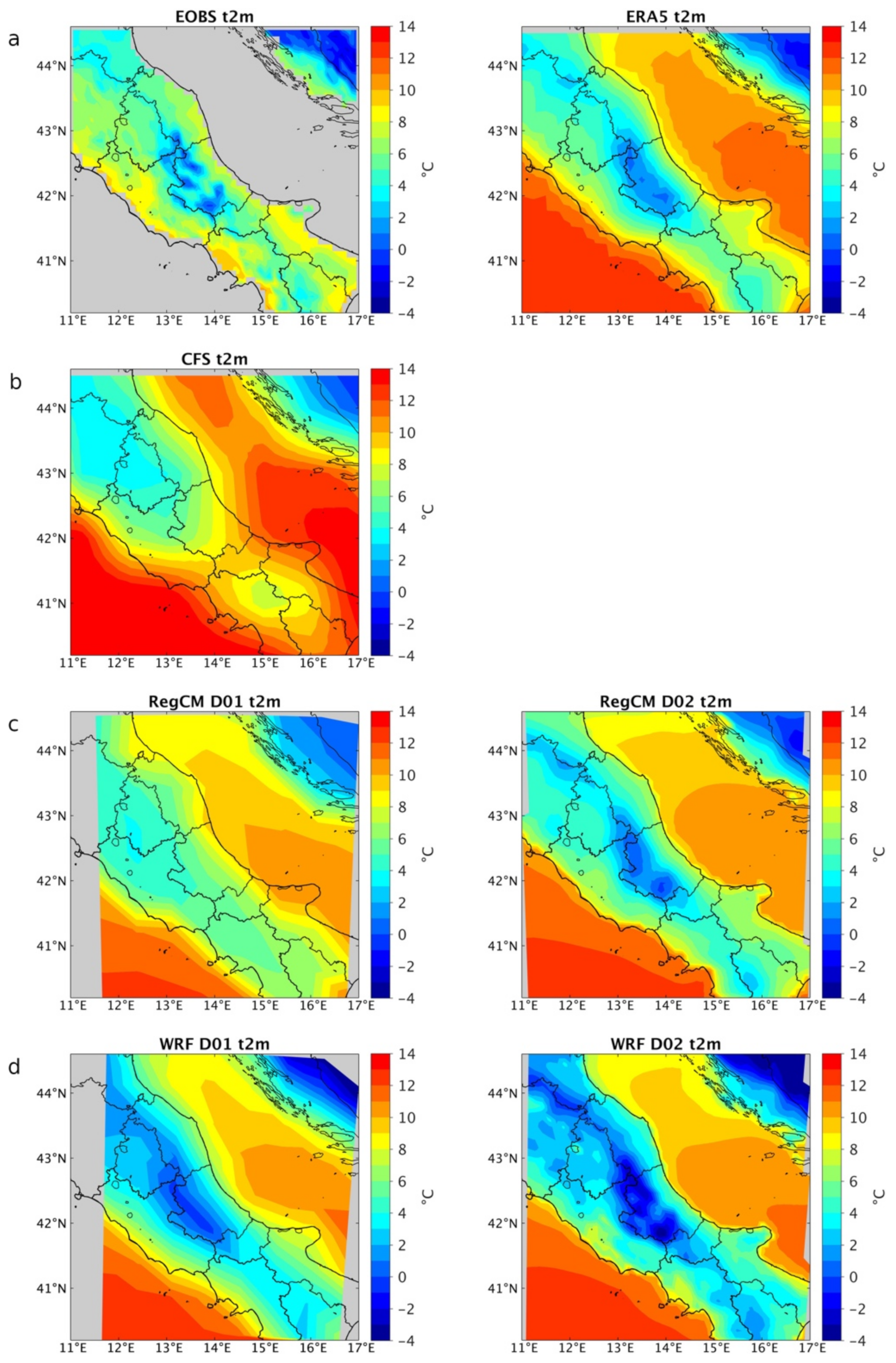
Figure 3 shows the spatial pattern of mean 2m temperature for the three SFSs and two reference products (EOBS and ERA5, Figure 3a). ERA5, if compared to EOBS, shows similar temperature values even though it fails to represent the topography-driven variation. This highlights that the ERA5 at 31 km resolution still has limitations in the representation of topography-dependent variables and its use as a reference product should be carefully evaluated in function of the specific case. CFS shows overall coherent temperature spatial patterns but, due to the coarse resolution, it obviously misses any topography-driven variability. Moving to the downscaled simulations, RegCM D01 is still ineffective in properly representing spatial patterns of temperature. D02 ensemble provides an expected improvement, showing values very similar to ERA5 and an improved representation of the topography-driven temperature variability. The two-step downscaling performed with WRF produces, to some extent, different results. Firstly, WRF ensemble introduces topography-induced temperature gradient already in the D01. This represents an interesting difference between the two regional-scale SFSs, and it is a sign of a different sensitivity to the topography of the two models, even if run at the same resolution and driven by the same global forcing. WRF D01 shows a clear improvement compared to the driving CFS, especially when compared to RegCM D01. However, we should also point out the WRF tendency to produce a temperature colder than the observed one regardless of the reference product considered. This can be seen especially at high resolution (WRF D02), where the 2 m temperature is further refined in accordance with an improved representation of topographical forcing and the cold biases are further enhanced, up to −4 °C if compared to the reference products. The high resolution (D02 runs) RegCM clearly produces more coherent temperature spatial patterns and physical values, showing biases that are generally around + or −1 °C all over the domain, and regardless of the reference product.
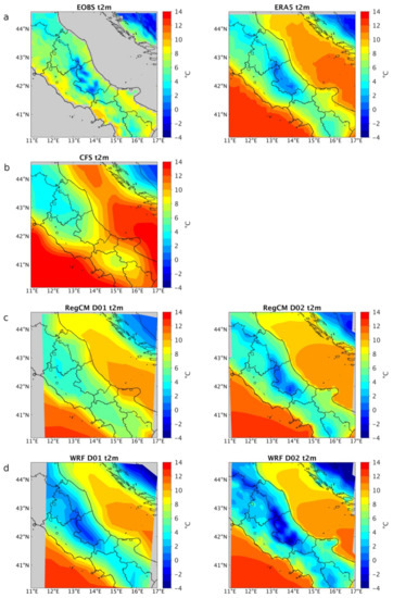
Figure 3.
Comparison of the climatologically averaged daily temperature over the reference period for (a) reference products EOBS and ECMWF ERA5. (b) Global-scale CFS. (c) RegCM D01 and D02 and (d) WRF D01 and D02.
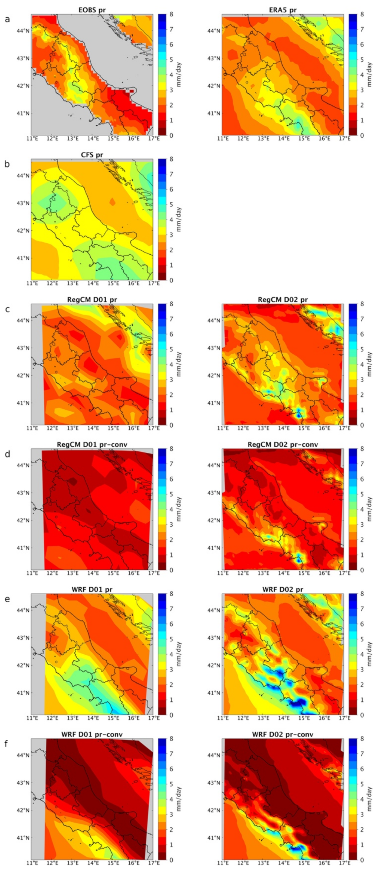
The same comparison applied to the temperature field is performed for the mean precipitation climatology (Figure 4). Interestingly, and differently from temperature, here we can notice large differences between the mean precipitation field provided by the two reference products. In fact, the area of maximum mean precipitation shows a similar magnitude but a different location. ERA5 shows a maximum over the coastline in the southwestern portion of the domain, while for EOBS a maximum is located further north following the Apennines Mountain ridge topography. Since the characterization of the reliability of the used reference products falls beyond this manuscript scope, we limit ourselves to recommend attention when choosing reference products, which of course can implicitly influence simulation validation results.
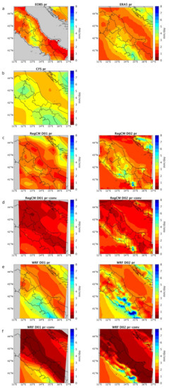
Figure 4.
Comparison of the climatologically averaged daily precipitation over the reference period for (a–c,e) total daily mean precipitation for reference products EOBS and ECMWF ERA5, CFS, RegCM (D01 and D02), WRF (D01 and D02), respectively. (d,f) convective component of the total precipitation for the RegCM (D01 and D02) and WRF (D01 and D02) respectively.
CFS (Figure 4b) produces a maximum precipitation dipole, while roughly reproducing what resulted from EOBS and ERA5. Again, while the physical values are overall coherent, we can clearly see the limitations imposed by the low resolution. Moving to the regional-scale SFSs, RegCM D01 (Figure 4c) produces a drier climatology clearly driven by the CFS field. On the other hand, the RegCM D02 clearly introduces spatial details and shows a maximum precipitation area, in a location similar to ERA5. Moreover, it produces larger precipitation patterns following the Apennines’ topography as outlined by EOBS. To get deeper inside the mechanisms for such a localized precipitation maximum, we further examine the regional-scale SFS precipitation, by decomposing data into total and convective precipitation components, in order to investigate the potential different dynamics in the two regional-scale SFS fields.
Figure 4c,d show that, for RegCM, the convective precipitation component is small in D01 while being the most relevant component in determining the precipitation maximum location in D02. WRF D01, as previously discussed for the temperature results, appears more sensitive to the topography forcing, when compared to the same resolution RegCM output. In fact, in Figure 4e, the precipitation shows a clear spatial pattern very similar to what seen in the ERA5. At the same time, WRF D02, as seen for the temperature, enhances the tendency seen in the driving D01. In Figure 4e, we can also see an excess of precipitation in the western Italian coast, especially in the south side. The WRF convective component (Figure 4f) plays a crucial role in determining precipitation maxima. However, differently from RegCM, where the convective precipitation component is only found at the D02 resolution, WRF convective component is already relevant at the D01 resolution. Finally, the signal of the convective component can be also found in ERA5 precipitation. Figure 1 of the Supplementary Materials (Figure S1) clearly shows an impact of the convective precipitation component in correspondence of precipitation maximum, similarly to what found in the two RCMs.
3.3. Analysis of Temperature and Precipitation Anomalies Interannual Variability
The results from the Anomaly Correlation Coefficients (ACCs) for the CFS and for the two regional-scale SFSs are presented in this section. In what follows, ERA5 is considered as a reference product. Even though ERA5 and EOBS show different climatologically averaged values (Figure 3a and Figure 4a), especially for the precipitation, they show similar results in terms of interannual variability of the anomalies (not shown).
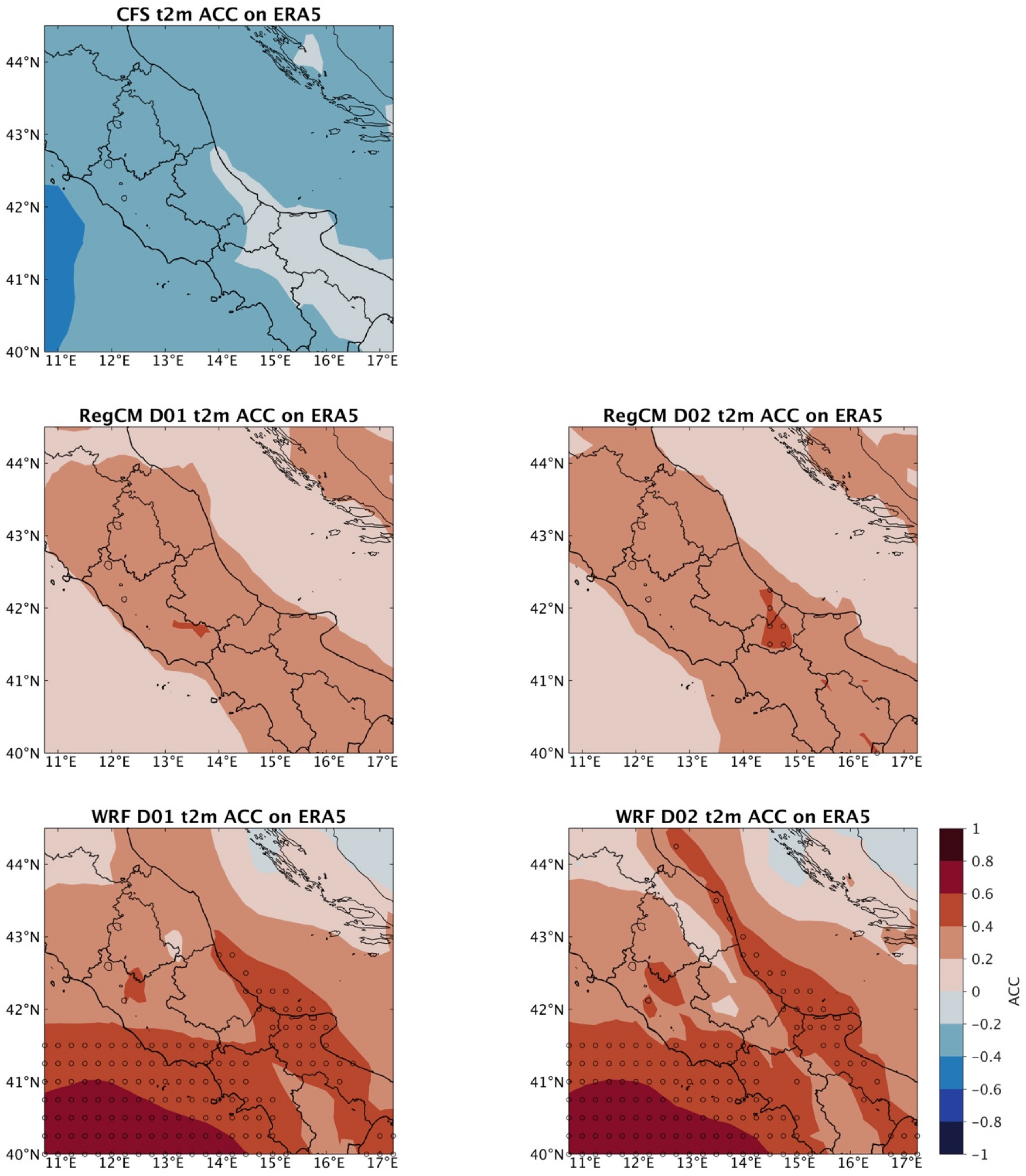
Figure 5 shows CFS characterized by negative ACCs. RegCM D01 improves the SAS of the temperature, especially over land points, showing positive ACCs. RegCM D02 shows mainly the same performance of the driving D01 field, while introducing significant positive ACC on a few inland grid nodes. Similarly, WRF improves the SAS-produced by the CFS by showing significantly positive ACC over a large portion of the domain. Moreover, a large positive ACC is found over the sea, which was not for RegCM. The further downscaling in WRF (D02) produces significant ACC on few additional grid points along the Adriatic coast, with respect to the D01.
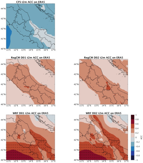
Figure 5.
Anomaly Correlation Coefficients (ACCs) for CFS upper panel, RegCM (D01 and D02) central panels and WRF (D01 and D02) bottom panels.
At this point it is worth focusing on the differences between the two RCM results. It can be observed that relevant ACCs improvement in WRF (both D01 and D02) characterizes the sea grid-points. Conversely, RegCM improves ACCs more over land points and less over sea points, even though the ACC field is generally not significant over the whole domain.
Resulting ACCs improvement pattern, combined to the absence of further improvement provided by the second downscaling, may suggest a relevant, though substantially different in the two RCMs, contribution from the driving pseudo-observed SST. However, the fact that the improvements in WRF occurs mostly over the sea does not necessarily mean that the model is mostly responsive to SST only. Land-sea processes can be coupled, and one can drive remote response, not just local ones.
Similarly, in the RegCM case, for which the improvement is not related to the SST grid nodes, it could well be that the model is overly responsive to land processes. Mechanisms-based analysis (e.g., evaporation, moisture and energy fluxes partitioning) would be needed to disentangle SST contribution from the different behavior of the two RCMs.
To the aim of further investigating these aspects, the ACC is computed according to different lead times to infer how the anomalies predictability is a function of forecast lead times (Figure S2). From this analysis we can observe large discrepancies among different lead times for the CFS, with the best performance in the 2-month lead time and with very poor performance in the 3-month lead time. Other two interesting aspects are related to the two RCMs. First, a confirmation of the very limited benefit obtained when moving from the D01 to the D02 grid resolution. Second, the presence of a large difference in the modulation of the CFS signal in the two RCMs. In this regard, WRF shows a clear connection to the signal coming from the CFS, following the large ACCs fluctuation among the different lead times. Additionally, in all the three lead times sea grid nodes show larger ACC improvement compared to land grid nodes. RegCM signal shows its best performance in the 1-month lead time and no strong connections with the driving CFS signal in all the three lead times.
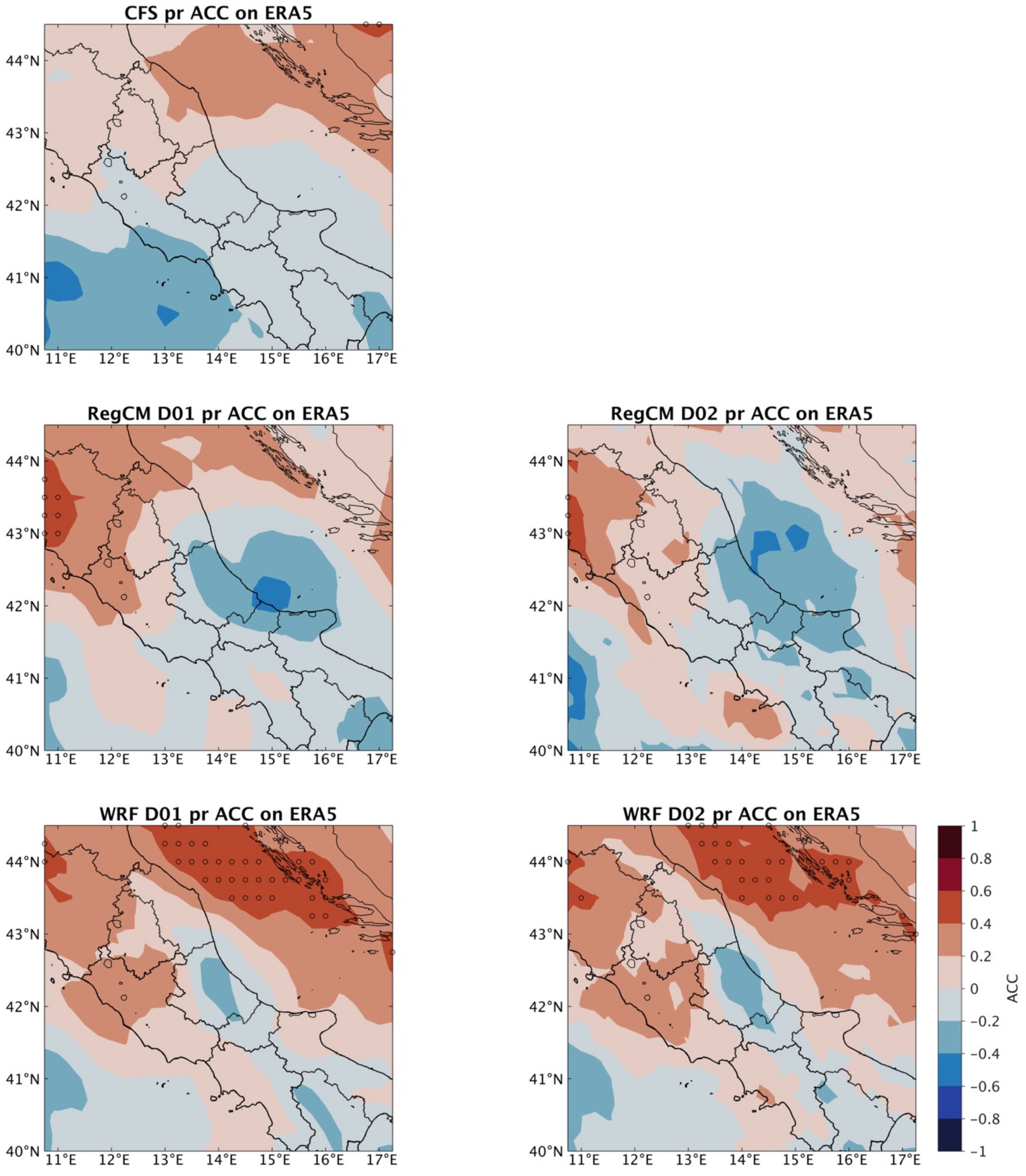
The precipitation ACCs (Figure 6), clearly shows a greater influence of CFS signal on the two RCM fields compared to what seen for the temperature.
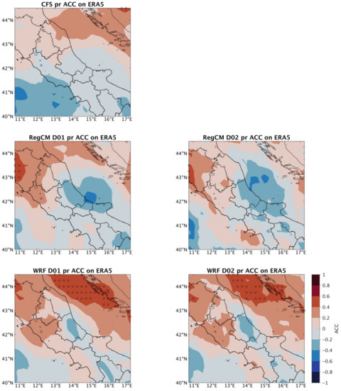
Figure 6.
Same as Figure 5 but for the precipitation.
The results show a sort of longitudinal gradient of anomalies predictability, with positive ACCs that are larger in the western part than in the eastern one, for the three SFSs. In general, WRF provides improvements that are larger than RegCM, regardless of resolution. Again, it is noteworthy that in both cases the higher resolution of the D02 runs does not provide benefit in terms of improving the interannual anomaly’s variability. If considering different lead times (Figure S3), we can see a degradation of CFS ACCs along the lead times with the lowest ACC field in February. Differently, the regional-scale SFSs do not show a clear dependency from the lead time considered. In the 2-month lead time we can notice an improvement of ACC produced by the RegCM D02 respect to the D01, and that WRF generally outperforms RegCM in the 1–2-month lead times.
3.4. Assessment of the Probabilistic Ensemble Forecasts
The ensemble mean is the most available metric for predicting future conditions, but it does not convey information regarding the prediction related uncertainty. The analysis of the distribution of the ensemble members represents a fundamental part of the information provided to the end-users about the potential outcome of a prediction. Probabilistic metrics are designed to characterize the predictive skill of an ensemble based SFS, taking into account probability distribution built on the forecasts produced by each ensemble member.
In this section the Continuous Ranked Probability Score (CRPS) performed considering the anomalies time series at each grid point, is used. All the simulations are preliminarily interpolated on the ERA5 grid, which is the reference product.
In order to provide the temporal variability of SFSs skill, CRPS is derived for each year and considering the spatial mean, following [39]:
where k represents each grid point of the D02 domain.
The minimum value of the difference between the predicted and occurred probability density functions, of the considered parameter, represents the best performing SFS. Figure 7 shows the spatial averaged CRPS for temperature and for each SFS, during the reference period. It can be observed that WRF shows, over almost all years, lower CRPS compared to RegCM. In turn, RegCM, though not systematically, improves the signal of CFS. Here, confirming ACC ensemble mean results, WRF seems to be able to outperform RegCM in reproducing SAS variability also through the probabilistic metric. Furthermore, other two aspects deserve to be considered. The first is that, as already seen in the ACCs metric, nothing seems to be gained in terms of skill when moving from D01 to D02 resolution in the two regional-scale SFSs. The second aspect is that both regional-scale SFSs show a CFS-dependent fluctuation along the reference period.

Figure 7.
D02 spatial averaged Continuous Ranked Probability Score (CRPS) for the CFS (blue), RegCM (red) and WRF (green). For RegCM and WF solid lines represent D01 simulations and doted lines D02 simulations.
Decomposing the CRPS results in the reliability and potential components, we can see that the WRF skill improvement mainly pertains to the reliability component. This feature indicates a better calibration of the WRF ensemble in terms of the equiprobability of finding the observed values among the different ensemble predicted values. If we consider the CRPS potential component and quantify the spread of the ensemble, different results are obtained. Firstly, WRF D02 shows poorer skill if compared to the driving D01, and to both RegCM resolutions, and also generally worsens CFS signal for the temperature. Differently, RegCM improves the CFS signal, similarly for both D01 and D02.
These latter results interestingly highlight that, even though well calibrated, WRF D02 ensemble is characterized by the larger spread, which represents a larger prediction uncertainty respect to RegCM and CFS. A summary of the temporal averaged CRPS and the related components is shown in Table 3.

Table 3.
Mean CRPS and related decomposition terms (reliability and potential) for CFS, RegCM and WRF SFSs.
The CRPS for the precipitation (Figure 8) shows a general improvement produced by the regional-scale SFSs, with the notable exception of year 2000 for WRF. Regarding the skill improvement provided by the further D02 downscaling, it can be observed (Table 3) that, in the case of RegCM, D02 worsens D01 CRPS, whereas WRF D02 slightly improves D01 CRPS. Again, it is noteworthy to investigate which of the two CRPS components plays a more relevant role in determining the total CRPS value. For the reliability component, RegCM consistently improves CFS, also outperforming the WRF for both D01 and D02. Regarding the CRPS potential component, the difference between RegCM D01 and D02 results has to be underlined. The RegCM D02 shows a higher CRPS potential, which is equivalent to a worsening, respect to D01 and CFS. This, in turn, leads to a total RegCM D02 CRPS poorer than the corresponding D01 value. As previously seen for the WRF ensemble in the case of temperature CRPS analysis, the higher resolution in the D02 runs produces a larger ensemble spread (i.e., a larger value of the CRPS potential component). Regarding the relative difference between D01 and D02, differently from RegCM, WRF D02 slightly outperforms D01 in both the CRPS components, yielding to a general higher skill.

Figure 8.
Same as Figure 7 but for the precipitation.
3.5. Percentile-Based Point-Scale Evaluation of Ensemble Forecasts
So far, only the means of physical values and related anomalies for both the deterministic and probabilistic analyses have been analyzed. For this analysis, a set of six representative measurement sites are selected from the Italian National Institute for Environmental Protection and Research (ISPRA) database [38]. The reasons behind the choice of additional reference data from observational sites are: (i) both observation-based and reanalysis gridded products have limitations in representing actual physical extreme values [35,36,37]. (ii) we aim to better isolate the effects of the downscaling, in terms of reproducibility of physical values and predictability of SAS variability.
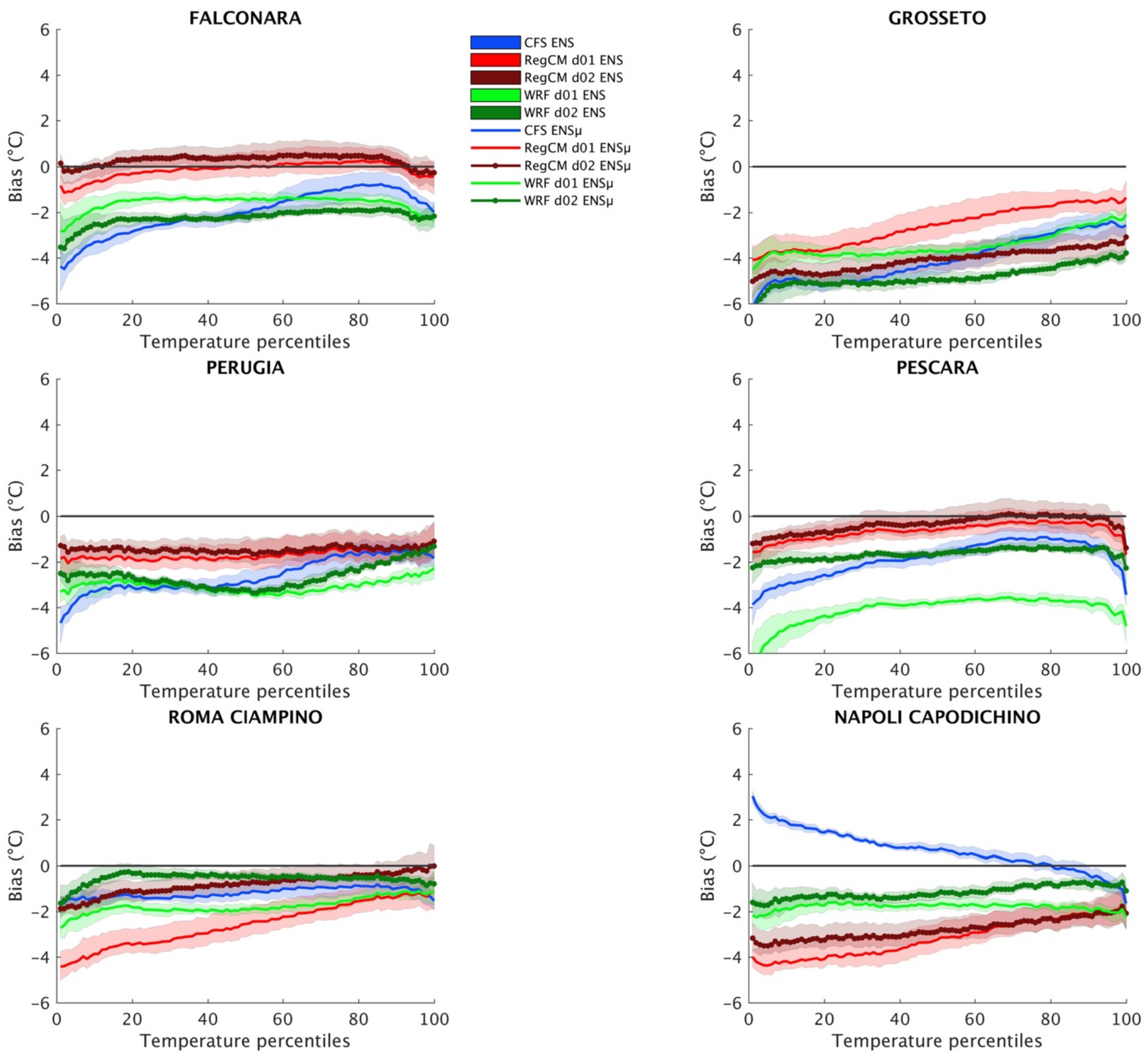
Figure 9 shows the mean biases for the whole distribution, over the reference period. For each reference site, the ensemble means (solid and dotted lines) and related all-member spread (shades) are plotted. For all the SFSs considered, cold biases prevail, with larger biases over lower percentiles. Considering the performance of the two regional-scale SFSs, percentile-based signal of CFS is not systematically improved. In general, the WRF ensemble seems to particularly worsen the driving CFS results. Even though with a large variability among reference sites, RegCM generally outperforms CFS and WRF along the entire statistical distribution, improving CFS signal on five out of six sites. Confirming previous results, no systematic improvement produced by the D02 with respect to the D01 can be noticed, for both the regional-scale SFSs.
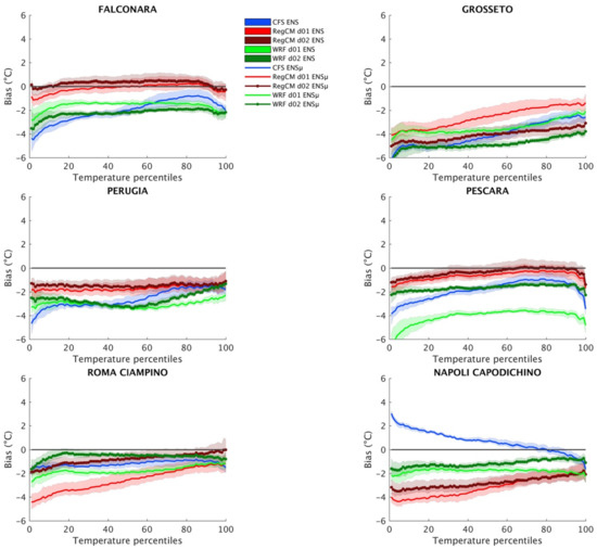
Figure 9.
Point-scale evaluation of the percentile-based reference period temperature for the CFS, RegCM and WRF SFSs. Shades represent all ensemble members variability solid lines ensemble means and dotted lines ensemble mean for the RegCM and WRF D02 simulations.
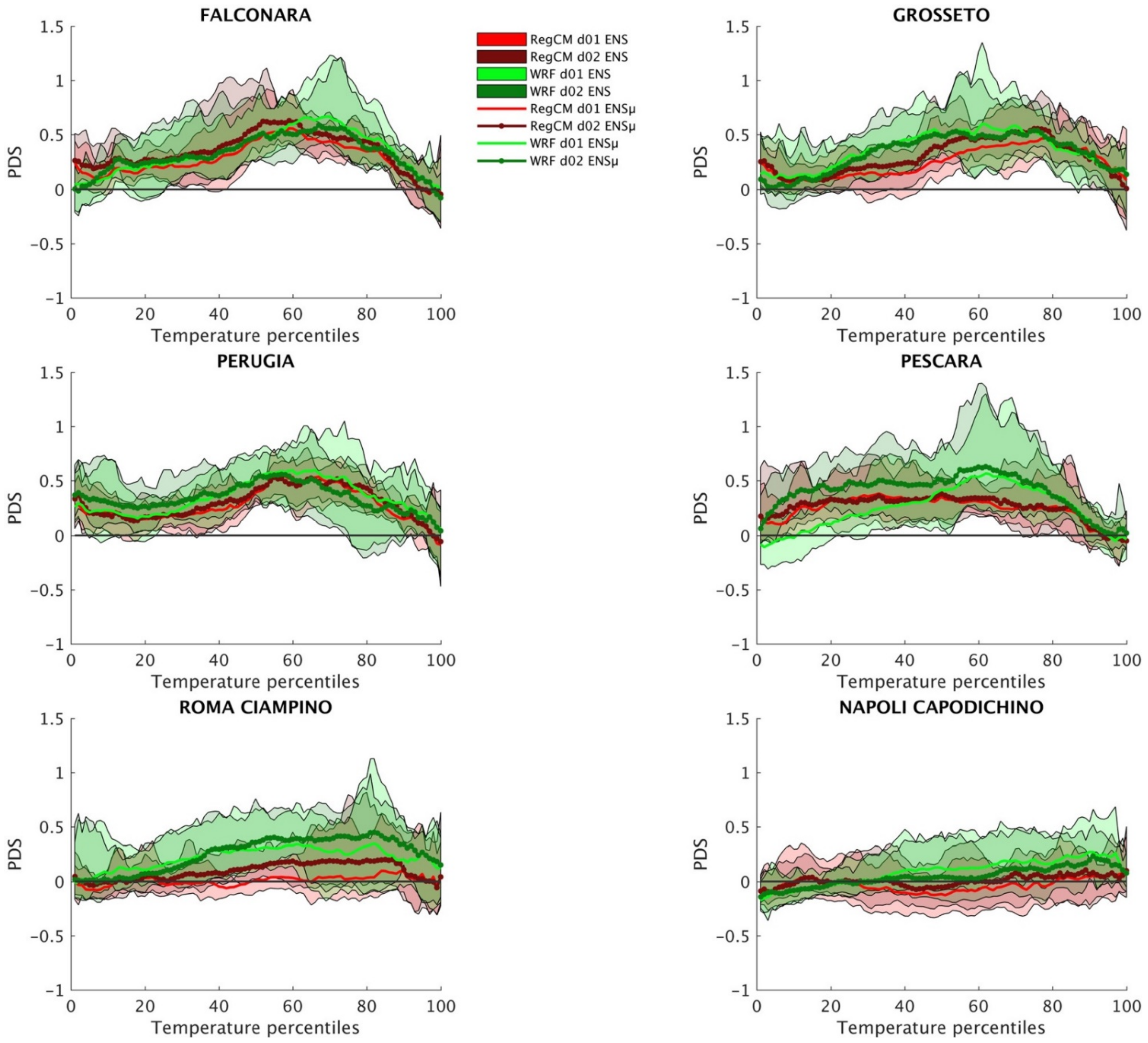
Figure 10 shows the results of the site-specific temperature PDS (defined in Section 2.2.4). A PDS constantly larger than zero indicates an improvement produced by the regional-scale SFSs over the driving CFS. Considering the ensemble mean PDS, WRF generally outperforms RegCM, with no remarkable difference between D01 and D02 runs. Regarding the statistical distribution, a larger PDS can be observed on the second and third quartiles of the distribution where PDS values for WRF members peak up to ~1.5. For the RegCM, D02 generally shows larger PDS respect to the D01.

Figure 10.
Same as Figure 9, but for the temperature percentile-based Downscaling Signal (PDS).
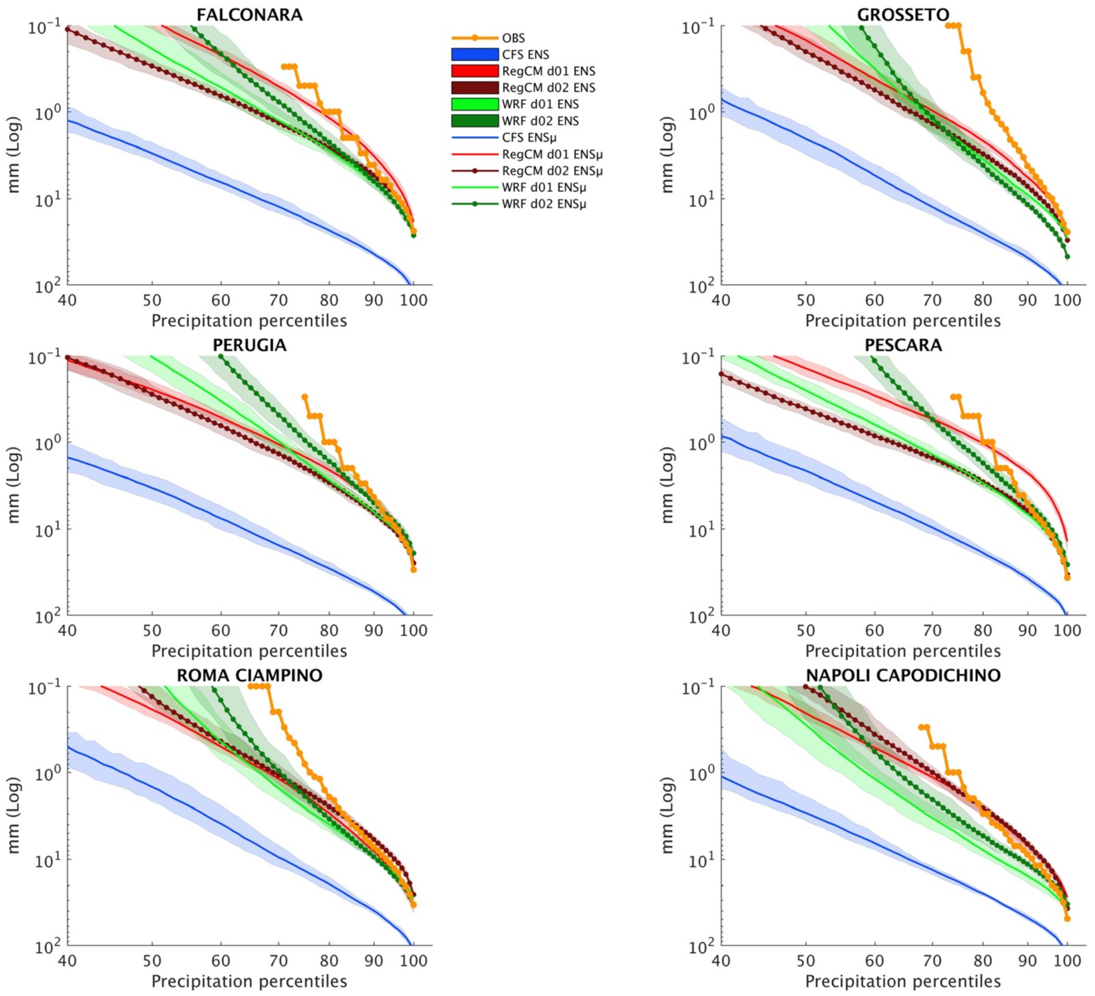
Figure 11 shows SFSs distribution biases for the precipitation over the reference sites. For the sake of readability, in the y-axes it is not reported the bias, as for the temperature, but the climatologically averaged daily precipitation for the three SFSs. The observation (orange dotted lines) is also shown. On the x-axis, the precipitation is cut at the 40th percentile, leaving out the “noisy” portion of precipitation distribution. All the SFSs show large biases over small precipitation amounts, while representing an excessive number of days with very light precipitation (<0.1 mm/day). This is particularly evident on the CFS for the reference sites. Looking at the median we can notice how this value shows larger precipitation amounts for the CFS. This means that very few dry days are simulated, compared to the other SFSs and the observation. Conversely, the observed precipitation thresholds of 0.1 or 0.2 mm/day are located around the 70th percentiles, indicating a consistently larger number of dry days within the reference period. At the opposite side of the distribution, we can see very large values produced by the CFS. Regional-scale SFSs converge toward observed values at the high percentiles, providing a consistent improvement over the driving CFS. RegCM and WRF perform similarly, with WRF D02 mainly outperforming D01. For the RegCM, the higher resolution D02 does not show improvement with respect to the D01.
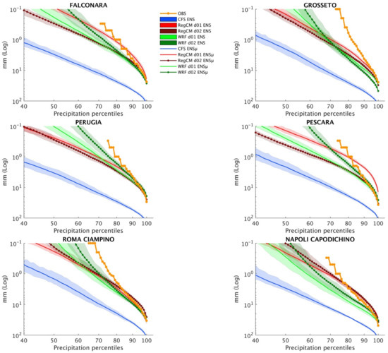
Figure 11.
Point-scale evaluation of the percentile-based reference period precipitation. Differently from FIG. 9 on y-axis is reported precipitation physical values instead of bias. Orange dotted lines represent observed precipitation.
Positive PDSs characterize all the reference sites also for precipitation data (Figure 12).
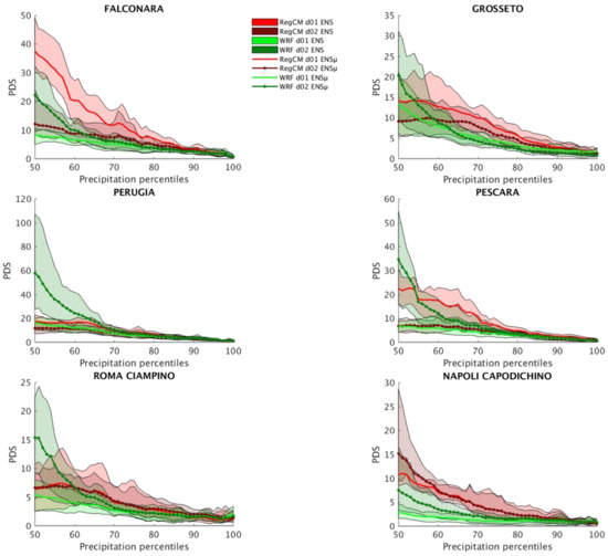
Figure 12.
Same as Figure 10, but for precipitation.
Similar to the previous analysis, we consider only the precipitation values above the median, in order to avoid “noisy” results determined by the presence of very small values within the computation of the PDS. The large improvement obtained in the first percentiles can be explained by recalling previous analysis (Figure 11), where the left portion of the CFS precipitation distribution shows very large values compared to the observation. Larger values in absolute terms tend to have quantitatively larger anomalies. These larger anomalies show larger MAE, when compared to the regional-scale SFSs. In fact, PDS approaches to zero on higher percentiles, where precipitation and related anomalies MAE values are closer. A zoom at higher percentiles (90th to 100th) PDS is shown in Figure 13, showing positive PDS values produced by the regional-scale SFSs over the highest values of precipitation.
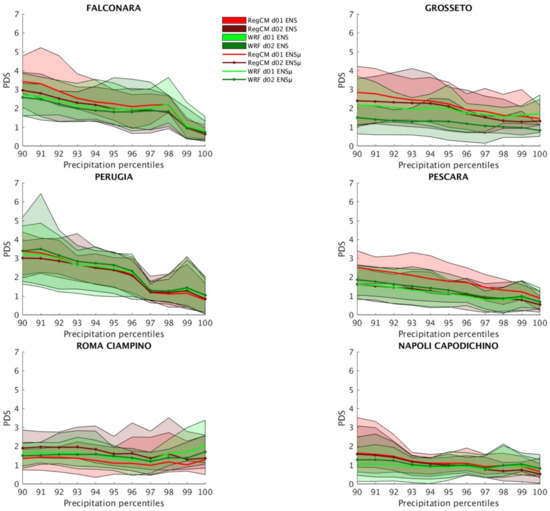
Figure 13.
Same as Figure 12, focusing on the 90th–100th percentiles.
4. Discussion and Conclusions
In this study, we have evaluated and compared the capability of two different dynamical downscaling approaches in improving a set of 21 winter season re-forecasts generated by the NCEP CFSv2, on a domain centered over Central Italy. Performance of the two regional-scale SFSs has been assessed by means of deterministic and probabilistic metrics, focusing on the capability of improving CFS SAS. The regional-scale SFSs consist of two-step dynamical downscaling performed by RegCM4.1 and WRF3.9.1.1 RCMs. The two RCMs are initially downscaled from a 100 km CFS resolution to a 60 km resolution over Southern Europe (D01). This first downscaling provides input fields for a further downscaling at a 12 km resolution over Central Italy (D02), which represents the main focus of the performed analysis. The two RCMs consider the same SST field as boundary condition.
As an initial analysis we have studied the spatial patterns of temperature and precipitation, climatologically averaged, physical values produced by the two-step downscaling, and compared them to the reference products represented by EOBS and ERA5. Results show that WRF introduces a sharper topography-driven temperature spatial distribution also in the D01 simulation, which is not the case for RegCM. However, WRF D01 temperature shows substantial cold biases down to −4 °C, regardless of the reference product considered. In the D02 simulations, WRF even enhances the cold bias found in the D01, whereas RegCM seems to better resolve the temperature spatial patterns, with biases generally in the range +/−1 °C.
For the precipitation fields, WRF shows a large sensitivity to the topography even at coarse resolution, whereas RegCM shows severe dry biases. As already found for the temperature, the D02 simulation for WRF produces very large values of the precipitation, with consistent wet biases compared to the two reference products. In comparison, RegCM D02 better reproduces the amount and the spatial patterns of the precipitation climatology.
For temperature ACCs, both the RCMs improve the driving CFS results, inverting ACCs field from negative to positive.
Other noteworthy differences between the two regional-scale SFSs are in the dependency from the signal produced by the driving CFS. If considering different lead times, WRF shows ACC variability related to CFS ACCs, whereas RegCM ACCs do not.
The ACCs for the precipitation in the two regional-scale SFSs are similar to the ones generated by the CFS, with only minor improvement, at both D01 and D02 resolutions. If considering different lead times, similarly to what observed for the temperature, WRF shows larger dependency from the CFS ACCs pattern.
The CRPS probabilistic metric for both WRF and RegCM regional-scale SFSs substantially improve CFS results, in terms of predictability of the anomaly interannual variability, with WRF clearly outperforming RegCM. However, it should be underlined that, from a decomposition of the CRPS value, WRF D02 is characterized by a larger mean spread corresponding to a higher level of uncertainty, compared to WRF D01 and to RegCM D01 and D02.
As already found for the temperature fields, also the regional-scale SFSs precipitation on D01 show an overall improvement of the skills, especially when considering the CRPS reliability component. The two regional-scale SFSs on D02 still show an improvement compared to CFS, with only WRF D02 producing a further improvement with respect to the D01 fields.
A point-scale evaluation of the ensemble forecasts, which considers individual grid nodes of the SFSs, for the temperature fields does not show a systematic improvement of the regional-scale SFSs compared to the driving CFS. However, RegCM generally outperforms WRF regardless of the resolution considered. The precipitation fields clearly show a skill improvement on both the low and high percentiles of the distribution.
For what concerns the temperature PDS metric, used to isolate the downscaling impact on the anomaly MAE, we can clearly see an improvement of the skill of the regional-scale SFSs on both D01 and D02, over all the reference sites. WRF generally seems to perform better than RegCM, but without any clear benefits when downscaling from D01 to D02. RegCM generally performs better on D02 compared to D01, over all the reference sites.
No clear results are found for the precipitation fields, which anyway show positive PDS over the entire statistical distribution.
When considering the temperature fields and both deterministic and probabilistic metrics, regional-scale SFSs consistently improve the original CFS SAS. For the precipitation, the added value of the regional-scale SFSs is mainly limited to the topography-driven refinement of the higher resolution precipitation field, whereas the resulting SAS is mainly “inherited” by the driving CFS. However, the regional-scale SFSs, performed with both RCMs, do not seem to benefit from the second downscaling (D01 to D02) in terms of CFS SAS improvement. In this regard, previous studies did document the benefit of dynamical downscaling in improving the climatology and interannual variability of precipitation when the resolution of the mesoscale model is refined to below 60 km. For example, [44,45] it appears that whether downscaling to the sub-mesoscale is useful depends on the specific regions (with different topography and large-scale climatological forcing). Similar to our findings, [45] in perfect-boundary-condition seasonal forecast configuration, found continued improvement in seasonal precipitation until the model resolution is refined to 36 km. Below it, the trend reverses, and the 12 km runs are worse than 36 km runs.
Along with the above-mentioned overall performance, we should also remark how WRF and RegCM nevertheless show substantial differences in the details of both the resulting SAS and climatologically averaged temperature and precipitation fields.
If we consider results from similar studies [27,28,29], performing a one-step downscaling (though at different resolutions, i.e., 25 km, 50 km and 50 km, respectively), where only marginal or no improvement of the SAS is found, compared to the driving field, we are led to speculate about the role played by the pseudo-observed SST, on determining CFS temperature SAS improvement which does not change when moving from D01 and D02, and impacts differently on the two RCMs. In WRF, significant positive ACCs characterizes mainly SST grid nodes. Conversely, RegCM reproduces higher ACCs over land. Though a relevant role played by a pseudo-observed SST (characterized by an inter-annual variability closer to the observed one) can be hypothesized, our findings are not sufficient to establish any direct relationship. Specific sensitivity analyses are required to disentangle SST influence and related differences observed between the two RCMs.
In light of the above findings and speculations, the next research step will be based on sensitivity experiments devoted to isolate and to quantify the role of the SST on the SAS predictability, from the global to the regional scale. The relevance of different RCMs initialization strategies can also be explored, e.g., [46,47]. This should also help in understanding the mechanisms behind the different response of the two RCMs to the same global-scale forcing, with particular regard to SST.
Supplementary Materials
The following are available online at https://www.mdpi.com/article/10.3390/atmos12060757/s1, Figure S1: Climatologically averaged daily convective component of the total precipitation for the ERA5 reanalysis; Figure S2: Anomaly Correlation Coefficients (ACCs) for the different seasonal forecasting systems CFS, RegCM (D01 and D02) and WRF (D01 and D02) for different lead times. Upper panels 1-month; central panels 2-month lead time and bottom panels 3-month lead time; Figure S3: Same as Figure S2 but for the precipitation.
Author Contributions
Conceptualization, L.S. and G.R.; methodology, L.S. and A.R.; formal analysis, L.S.; investigation, L.S. and A.R.; resources, L.S., G.R. and R.F.; data curation, L.S.; writing—original draft preparation, L.S.; writing—review and editing, G.R. and R.F.; visualization, L.S.; supervision, G.R. and R.F.; funding acquisition, R.F. and L.S. All authors have read and agreed to the published version of the manuscript.
Funding
This research was funded by PON Ricerca e Innovazione 2014–2020 “AIM”—Attraction and international mobility program. EU Social Fund and Regional Development Fund; Ministero dell’Istruzione e della Ricerca, grant number AIM1858058.
Institutional Review Board Statement
Not applicable.
Informed Consent Statement
Not applicable.
Data Availability Statement
Seasonal climate simulation datasets are available upon request to the lead author.
Acknowledgments
The authors acknowledge the European Union’s Earth observation programme Copernicus and the Italian Istituto Superiore per la Protezione e la Ricerca Ambientale (ISPRA) for making available reference datasets used in this study. The authors also want to thank the National Centers for Environmental Prediction for making publicly available the NCEP Climate Forecast System Version (https://nomads.ncdc.noaa.gov/modeldata/) which have been used in this study as initial and boundary conditions for the dynamical downscaling. The authors would also like to thank the International Centre for Theoretical Physics (ICTP) for making publicly available climate model RegCM code which has been compiled and run on the internal computing resources at CETEMPS (University of L’Aquila). L.S. thanks to the CINECA-ISCRA Italian Super Computing Resource on which WRF numerical simulations have been performed (project: CPSWCM–HP10BRUALV).
Conflicts of Interest
The authors declare that they have no conflict of interest.
References
- Doblas-Reyes, F.J.; García-Serrano, J.; Lienert, F.; Biescas, A.P.; Rodrigues, L.R.L. Seasonal climate predictability and forecasting: Status and prospects. Wiley Interdiscip. Rev. Clim. Chang. 2013, 4, 245–268. [Google Scholar] [CrossRef]
- Goddard, L.; Hurrell, J.W.; Kirtman, B.P.; Murphy, J.; Stockdale, T.; Vera, C. Two time scales for the price of one (almost). Bull. Am. Meteorol. Soc. 2012, 93, 621–629. [Google Scholar] [CrossRef]
- Molteni, F.; King, M.P.; Kucharski, F.; Straus, D.M. Planetary-scale variability in the northern winter and the impact of land-sea thermal contrast. Clim. Dyn. 2011, 37, 151–170. [Google Scholar] [CrossRef]
- Saha, S.; Moorthi, S.; Wu, X.; Wang, J.; Nadiga, S.; Tripp, P.; Behringer, D.; Hou, Y.; Chuang, H.; Iredell, M.; et al. The NCEP Climate Forecast System Version. J. Clim. 2014, 3, 2185–2208. [Google Scholar] [CrossRef]
- Maclachlan, C.; Arribas, A.; Peterson, K.A.; Maidens, A.; Fereday, D.; Scaife, A.A.; Gordon, M.; Vellinga, M.; Williams, A.; Comer, R.E.; et al. Global Seasonal forecast system version 5 (GloSea5): A high-resolution seasonal forecast system. Q. J. R. Meteorol. Soc. 2015, 141, 1072–1084. [Google Scholar] [CrossRef]
- Befort, D.J.; Wild, S.; Knight, J.R.; Lockwood, J.F.; Thornton, H.E.; Hermanson, L.; Bett, P.E.; Weisheimer, A.; Leckebusch, G.C. Seasonal forecast skill for extratropical cyclones and windstorms. Q. J. R. Meteorol. Soc. 2019, 145, 92–104. [Google Scholar] [CrossRef]
- Alexander, M.A.; Bladé, I.; Newman, M.; Lanzante, J.R.; Lau, N.C.; Scott, J.D. The atmospheric bridge: The influence of ENSO teleconnections on air-sea interaction over the global oceans. J. Clim. 2002, 15, 2205–2231. [Google Scholar] [CrossRef]
- Mariotti, A.; Struglia, M.V.; Zeng, N.; Lau, K.-M. The Hydrological Cycle in the Mediterranean Region and Implications for the Water Budget of the Mediterranean Sea. J. Clim. 2002, 15, 1674–1690. [Google Scholar] [CrossRef]
- Molteni, F.; Stockdale, T.; Balmaseda, M.; Balsamo, G.; Buizza, R.; Ferranti, L.; Magnusson, L.; Mogensen, K.; Palmer, T.; Vitart, F. The New ECMWF Seasonal Forecast System (System 4); ECMWF Technical Memoranda No. 656; European Centre for Medium Range Weather Forecasts: Berkshire, UK, 2011; 49p. [Google Scholar]
- Grassi, B.; Redaelli, G.; Visconti, G. Arctic sea ice reduction and extreme climate events over the mediterranean region. J. Clim. 2013, 26, 10101–10110. [Google Scholar] [CrossRef]
- Weisheimer, A.; Befort, D.J.; Macleod, D.; Palmer, T.; Reilly, C.O.; Strømmen, K. Seasonal Forecasts of the Twentieth Century. Bull. Am. Meteorol. Soc. 2020, 101, 1413–1426. [Google Scholar] [CrossRef]
- Bruno Soares, M.; Dessai, S. Exploring the use of seasonal climate forecasts in Europe through expert elicitation. Clim. Risk Manag. 2015, 10, 8–16. [Google Scholar] [CrossRef]
- Buontempo, C.; Hewitt, C.D.; Doblas-Reyes, F.J.; Dessai, S. Climate service development, delivery and use in Europe at monthly to inter-annual timescales. Clim. Risk Manag. 2014, 6, 1–5. [Google Scholar] [CrossRef]
- Coppola, E.; Sobolowski, S.; Pichelli, E.; Raffaele, F.; Ahrens, B.; Anders, I.; Ban, N.; Bastin, S.; Belda, M.; Belusic, D.; et al. A First-of-Its-Kind Multi-Model Convection Permitting Ensemble for Investigating Convective Phenomena over Europe and the Mediterranean; Springer: Berlin/Heidelberg, Germany, 2018; ISBN 0123456789. [Google Scholar]
- Giorgi, F.; Jones, C.; Asrar, G.R. Addressing climate information needs at the regional level: The CORDEX framework. WMO Bull. 2009, 58, 175–183. [Google Scholar]
- Van der Lindend, P.; Mitchell, J.F.B. Climate Change and Its Impacts: Summary of Research and Results from the ENSEMBLES Project; Met Office Hadley Centre: Exeter, UK, 2009. [Google Scholar]
- Palmer, T.N.; Alessandri, A.; Andersen, U.; Cantelaube, P.; Davey, M.; Délécluse, P.; Déqué, M.; Díez, E.; Doblas-Reyes, F.J.; Feddersen, H.; et al. Development of a European multimodel ensemble system for seasonal-to-interannual prediction (DEMETER). Bull. Am. Meteorol. Soc. 2004, 85, 853–872. [Google Scholar] [CrossRef]
- Pal, S.; Chang, H.I.; Castro, C.L.; Dominguez, F. Credibility of convection-permitting modeling to improve seasonal precipitation forecasting in the southwestern United States. Front. Earth Sci. 2019, 7. [Google Scholar] [CrossRef]
- De Sales, F.; Xue, Y. Dynamic downscaling of 22-year CFS winter seasonal hindcasts with the UCLA-ETA regional climate model over the United States. Clim. Dyn. 2013, 41, 255–275. [Google Scholar] [CrossRef]
- Castro, C.L.; Chang, H.I.; Dominguez, F.; Carrillo, C.; Schemm, J.K.; Juang, H.M.H. Can a regional climate model improve the ability to forecast the North American monsoon? J. Clim. 2012, 25, 8212–8237. [Google Scholar] [CrossRef]
- Fennessy, M.J.; Shukla, J. Seasonal prediction over North America with a regional model nested in a global model. J. Clim. 2000, 13, 2605–2627. [Google Scholar] [CrossRef]
- Nikulin, G.; Asharaf, S.; Magariño, M.E.; Calmanti, S.; Cardoso, R.M.; Bhend, J.; Fernández, J.; Frías, M.D.; Fröhlich, K.; Früh, B.; et al. Dynamical and statistical downscaling of a global seasonal hindcast in eastern Africa. Clim. Serv. 2018, 9, 72–85. [Google Scholar] [CrossRef]
- Siegmund, J.; Bliefernicht, J.; Laux, P.; Kunstmann, H. Toward a seasonal precipitation prediction system for West Africa: Performance of CFSv2 and high-resolution dynamical downscaling. J. Geophys. Res. 2015, 120, 7316–7339. [Google Scholar] [CrossRef]
- Diro, G.T.; Tompkins, A.M.; Bi, X. Dynamical downscaling of ECMWF Ensemble seasonal forecasts over East Africa with RegCM. J. Geophys. Res. Atmos. 2012, 117, 1–20. [Google Scholar] [CrossRef]
- Phan Van, T.; Van Nguyen, H.; Trinh Tuan, L.; Nguyen Quang, T.; Ngo-Duc, T.; Laux, P.; Nguyen Xuan, T. Seasonal Prediction of Surface Air Temperature across Vietnam Using the Regional Climate Model Version 4.2 (RegCM4.2). Adv. Meteorol. 2014, 2014, 245104. [Google Scholar] [CrossRef]
- Yuan, X.; Liang, X.Z.; Wood, E.F. WRF ensemble downscaling seasonal forecasts of China winter precipitation during 1982–2008. Clim. Dyn. 2012, 39, 2041–2058. [Google Scholar] [CrossRef]
- Manzanas, R.; Lucero, A.; Weisheimer, A.; Gutiérrez, J.M. Can bias correction and statistical downscaling methods improve the skill of seasonal precipitation forecasts? Clim. Dyn. 2018, 50, 1161–1176. [Google Scholar] [CrossRef]
- Díez, E.; Orfila, B.; Frías, M.D.; Fernández, J.; Cofiño, A.S.; Gutiérrez, J.M. Downscaling ECMWF seasonal precipitation forecasts in Europe using the RCA model. Tellus Ser. A Dyn. Meteorol. Oceanogr. 2011, 63, 757–762. [Google Scholar] [CrossRef]
- Patarčić, M.; Branković, Č. Skill of 2-m Temperature Seasonal Forecasts over Europe in ECMWF and RegCM Models. Mon. Weather Rev. 2011, 140, 1326–1346. [Google Scholar] [CrossRef]
- Ferretti, R.; Lombardi, A.; Tomassetti, B.; Sangelantoni, L.; Colaiuda, V.; Mazzarella, V.; Maiello, I.; Verdecchia, M.; Redaelli, G. A meteorological-hydrological regional ensemble forecast for an early-warning system over small Apennine catchments in Central Italy. Hydrol. Earth Syst. Sci. 2020, 24, 3135–3156. [Google Scholar] [CrossRef]
- Sangelantoni, L.; Ferretti, R.; Redaelli, G. Toward a Regional-Scale Seasonal Climate Prediction System over Central Italy based on Dynamical Downscaling. Climate 2019, 7, 120. [Google Scholar] [CrossRef]
- Sangelantoni, L.; Mazzarella, V.; Ricchi, A.; Ferretti, R. Toward A Regional-Scale Seasonal Climate Prediction System over the Mediterranean Basin: Evaluation and Comparison of RegCM- and WRF-Based Dynamical Downscaling Approaches. In Proceedings of the EGU General Assembly Conference Abstracts, Online, 4–8 May 2020; p. 10557. [Google Scholar]
- Reynolds, R.W.; Rayner, N.A.; Smith, T.M.; Stokes, D.C.; Wang, W. An improved in situ and satellite SST analysis for climate. J. Clim. 2002, 15, 1609–1625. [Google Scholar] [CrossRef]
- Ricchi, A.; Miglietta, M.M.; Bonaldo, D.; Cioni, G.; Rizza, U.; Carniel, S. Multi-Physics ensemble versus atmosphere-ocean coupled model simulations for a tropical-like cyclone in the Mediterranean Sea. Atmosphere 2019, 10, 202. [Google Scholar] [CrossRef]
- Haylock, M.; Hofstra, N.; Klein Tank, A.; Klok, E.; Jones, P. A European daily high-resolution gridded data set of surface temperature and precipitation for 1950–2006. J. Geophys. Res. Atmos. 2008, 113. [Google Scholar] [CrossRef]
- Hofstra, N.; Haylock, M.; New, M.; Jones, P.D. Testing E-OBS European high-resolution gridded data set of daily precipitation and surface temperature. J. Geophys. Res. Atmos. 2009, 114. [Google Scholar] [CrossRef]
- Hersbach, H.; Bell, B.; Berrisford, P.; Hirahara, S.; Horányi, A.; Muñoz-Sabater, J.; Nicolas, J.; Peubey, C.; Radu, R.; Schepers, D.; et al. The ERA5 global reanalysis. Q. J. R. Meteorol. Soc. 2020, 146, 1999–2049. [Google Scholar] [CrossRef]
- Desiato, F.; Fioravanti, G.; Fraschetti, P.; Perconti, W.; Toreti, A. Climate indicators for Italy: Calculation and dissemination. Adv. Sci. Res. 2011, 6, 147–150. [Google Scholar] [CrossRef]
- Hersbach, H. Decomposition of the continuous ranked probability score for ensemble prediction systems. Weather Forecast. 2000, 15, 559–570. [Google Scholar] [CrossRef]
- Mishra, N.; Prodhomme, C.; Guemas, V. Multi-model skill assessment of seasonal temperature and precipitation forecasts over Europe. Clim. Dyn. 2019, 52, 4207–4225. [Google Scholar] [CrossRef]
- Pappenberger, F.; Ramos, M.H.; Cloke, H.L.; Wetterhall, F.; Alfieri, L.; Bogner, K.; Mueller, A.; Salamon, P. How do I know if my forecasts are better? Using benchmarks in hydrological ensemble prediction. J. Hydrol. 2015, 522, 697–713. [Google Scholar] [CrossRef]
- Zhao, T.; Chen, H.; Xu, W.; Cai, H.; Yan, D.; Chen, X. Spatial association of anomaly correlation for GCM seasonal forecasts of global precipitation. Clim. Dyn. 2020. [Google Scholar] [CrossRef]
- Grillakis, M.; Koutroulis, A.; Tsanis, I. Improving seasonal forecasts for basin scale hydrological applications. Water 2018, 10, 1593. [Google Scholar] [CrossRef]
- Lindstedt, D.; Lind, P.; Kjellström, E.; Jones, C. A new regional climate model operating at the meso-gamma scale: Performance over Europe. Tellus Ser. A Dyn. Meteorol. Oceanogr. 2015, 67. [Google Scholar] [CrossRef]
- Sharma, A.; Huang, H.P. Regional Climate Simulation for Arizona: Impact of Resolution on Precipitation. Adv. Meteorol. 2012, 2012. [Google Scholar] [CrossRef]
- De Luca, D.L. Analysis and modelling of rainfall fields at different resolutions in southern Italy. Hydrol. Sci. J. 2014, 59, 1536–1558. [Google Scholar] [CrossRef]
- Hu, H.; Ayyub, B.M. Validating and enhancing extreme precipitation projections by downscaled global climate model results and copula methods. J. Hydrol. Eng. 2019, 24, 04019019. [Google Scholar] [CrossRef]
Publisher’s Note: MDPI stays neutral with regard to jurisdictional claims in published maps and institutional affiliations. |
© 2021 by the authors. Licensee MDPI, Basel, Switzerland. This article is an open access article distributed under the terms and conditions of the Creative Commons Attribution (CC BY) license (https://creativecommons.org/licenses/by/4.0/).


