Long-Term Variations of Global Solar Radiation and Atmospheric Constituents at Sodankylä in the Arctic

Abstract

An empirical model of global solar irradiance (EMGSI) under all sky conditions was developed by using solar radiation and meteorological parameters at Sodankylä. The calculated hourly global solar irradiance is in agreement with that observed at the ground during 2008–2011 and at the top of the atmosphere (TOA). This model is used to calculate the global solar irradiance at the ground and its attenuation in the atmosphere due to absorbing and scattering substances in 2000–2018. The sensitivity test indicates that the responses of global solar irradiance to changes in water vapor and scattering factors are nonlinear and negative, and global solar irradiance is more sensitive to changes in scattering (expressed by the scattering factor S/G, S and G are diffuse and global solar radiation, respectively) than to changes in water vapor. Using this empirical model, we calculated the albedos at the TOA and the surface, which are in agreement with the satellite-retrieved values. A good relationship between S/G and aerosol optical depth (AOD) was determined and used to estimate AOD in 2000–2018. An empirical model for estimation of tropospheric NO₂ vertical column density (VCD) was also developed and used to calculate tropospheric NO₂ VCD in 2000–2018. During 2000–2018, the estimated global solar irradiance decreased by 0.92%, and diffuse irradiance increased by 1.28% per year, which is ascribed to the increases of S/G (1.73%) and water vapor (0.43%). Annual surface air temperature increases by 0.07 °C per year. Annual mean loss of global solar irradiance caused by absorbing and scattering substances and total loss are 1.94, 1.17 and 3.11 MJ m⁻², respectively. Annual mean losses of absorbing and scattering global solar irradiance show negative and positive trends, respectively, and the annual total loss increases by 0.24% per year. Annual mean losses due to absorption were much larger than those due to scattering. The calculated albedos at the TOA are smaller than at the surface. The calculated and satellite-retrieved annual albedos decrease at the TOA and increase at the surface. During 2000–2018, annual means of the AOD and the tropospheric NO₂ VCD increased by 8.23% and 0.03% per year, respectively.

1. Introduction

The surface temperatures in the Arctic increase much faster than the global average, a phenomenon known as Arctic Amplification. The most significant increase occurs in the winter [1,2,3]. The Arctic warming is related to the imbalance of energy budget at the ground and the top of the atmosphere (TOA), sea-ice–albedo feedback, lapse-rate feedback, temperature inversion, enhanced greenhouse effect [1] and the reasons for the climate change in the Arctic region are still unclear.

The Sun provides important energy to the atmospheric gases, liquids and particles (GLPs) and initiates their changes in the three phases through chemical and photochemical reactions (CPRs). Therefore, solar radiation transfers in and interacts with the atmospheric GLPs. The attenuation in the atmosphere and reflections at the ground and the TOA are necessary to be investigated; these physical and chemical processes control/interact with the atmospheric movement through short- and long-wave radiation in different ways [4,5,6,7,8,9,10,11,12], and should be studied for further understanding the regional climate and climate change in the Arctic.

The popular radiative transfer models and empirical models are used to estimate global, direct and diffuse solar radiation at the ground and briefly described in References [12,13,14,15,16,17,18,19,20]. To thoroughly investigate the Sun–atmosphere–Earth system, variations of solar radiation at the surface and the TOA, the loss of solar radiation in the atmosphere, the albedos at the surface and the TOA, and the interactions between solar radiation and meteorological variables are required. The objectives of this study were to study (1) global solar radiation at the surface and the TOA; (2) the distribution of the absorbing and scattering losses of global solar radiation in the atmosphere, and their relations with the atmospheric substances and meteorological parameters; (3) albedos at the TOA and the surface; (4) the relationships between absorbing and scattering energy and their affecting factors; (5) aerosol optical depth (AOD); (6) tropospheric NO₂ vertical column densities (VCDs); and (7) long-term variations and integrated effects of above variables. Solar radiation and meteorological variables observed over four years were used to develop an empirical model of global solar irradiance at Sodankylä in the Arctic (Section 2.1 and Section 2.2). This model was applied to evaluate the above aims 1–7, and the results at Sodankylä were compared with one site in mid-latitude (Section 3 and Section 4) to better understand the basic properties of the Sun–atmosphere–Earth system extensively.

2. Data and Methodology

2.1. Observations and Data Selection

The measurements of solar radiation and meteorological variables were obtained at Sodankylä station (67.367 N, 26.630 E, 184 m a.s.l.), Finland, from January 2001 to December 2018. Global solar irradiance (GHI, 285–2800 nm, expressed as Q) and diffuse horizontal irradiance (DHI, expressed as S) were measured by pyranometers CM11 and CM11 with a 2AP-GD Sun tracker (Kipp & Zonen Inc., Delft, The Netherlands). Meteorological parameters, including air temperature (T), relative humidity (RH) and wind speed (v), were measured by using sensors, Model Pt100, (Pentronic Inc., Västervik, Sweden), Model HMP45D (Vaisala Inc., Vantaa, Finland) and Model UA2D (Adolf Thies GMBH & CO, Göttingen, Germany), respectively. The areas surrounding the Sodankylä station are covered by boreal coniferous forest and peatlands. Snow covers the ground from October to April, and minimum and maximum temperatures reach −40 and +30 °C [21,22,23].

Large cosine errors occur at a low solar elevation angle, and the observed hourly global solar radiation larger than 20 W m⁻² was used in the analysis and then to obtain the daily and monthly averages. The extreme hourly values of irradiances (G, S and D), together with the abnormal ratios of S/G, were removed in the analysis. The observed hourly maxima of global and direct solar radiation were less than extraterrestrial radiation. This data quality is generally in line with the measured solar radiation data, ranging from 0 to 1.2 times the extraterrestrial radiation [24].

Hourly solar irradiance and meteorological variables during 2008–2011 were selected to develop an empirical model of solar global irradiance under all sky conditions.

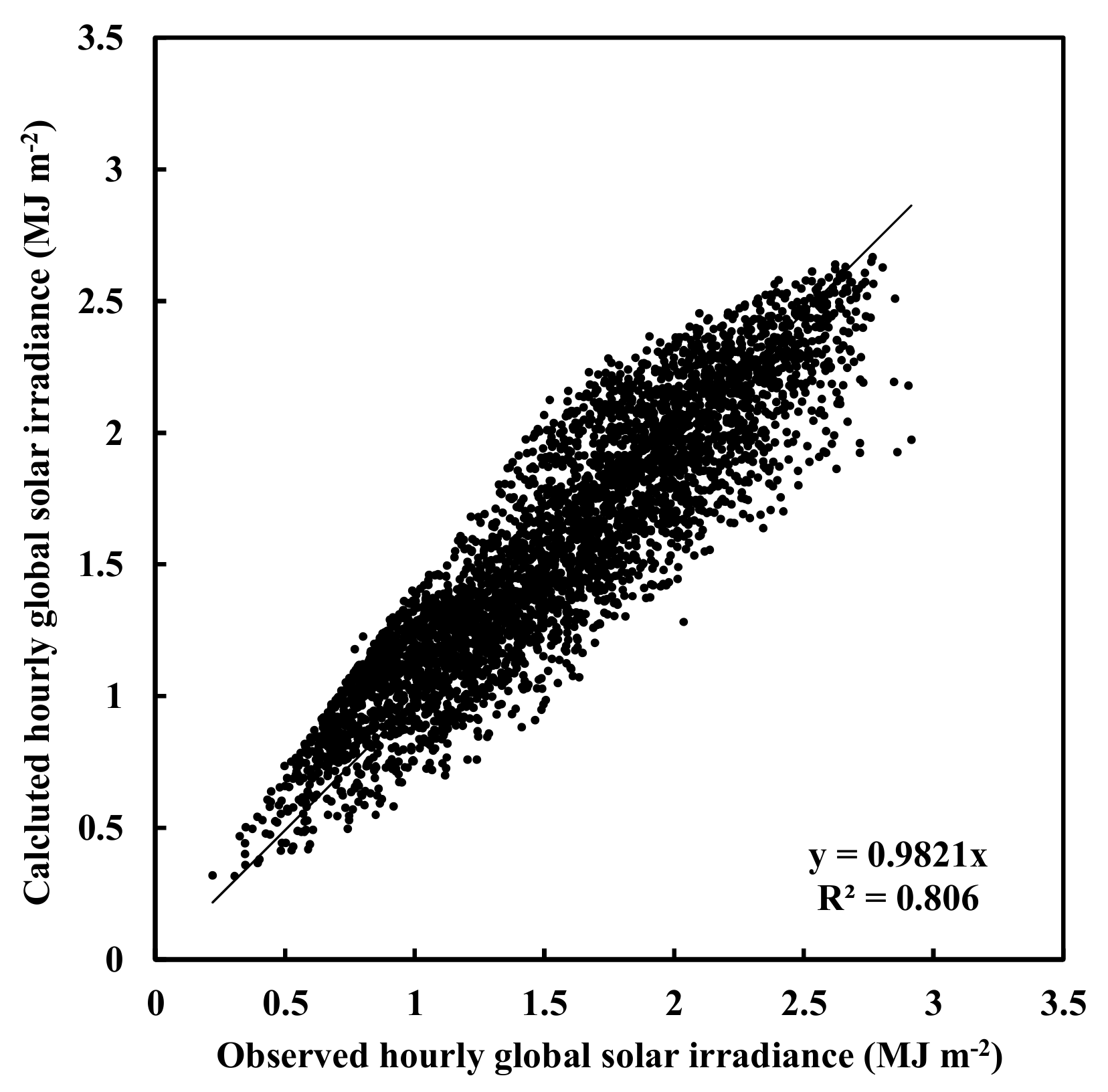
2.2. Model Formulation, Development and Evaluation

When global solar radiation transfers in the atmosphere, the absorbing and scattering processes are considered [12]: (1) Absorption, total absorption and use of global solar radiation by GLPs, is described as e^−kWm×cos(Z); k is the mean absorption coefficient of water vapor (0.70–2.845 μm), W is the water vapor content in the atmospheric column (cm), W = 0.02 E × 30 [25], E is the water vapor pressure (hPa), m is the optical air mass in the middle of each hour and Z is solar zenith angle (degree). The meaning and mechanism of this term (including direct absorption and indirect use of the light) in the UV, visible and near-infrared wavelength regions are fully discussed in Reference [12], especially the important roles that GLP play in CPRs associating with volatile organic compounds (VOCs) and OH radicals. (2) Scattering, total scattering of global solar radiation by GLPs, is expressed as e^−S/G. Then, an empirical model of global solar irradiance at a horizontal plane was applied in the Arctic for all sky conditions [12]:

$$\mathrm{G}{\mathrm{cal}}_{ }={{\mathrm{A}}_1\mathrm{e}}^{-\mathrm{kWm}}\times \cos \left(\mathrm{Z}\right)+{{\mathrm{A}}_{2}e}^{-\mathrm{S}/{\mathrm{G}}_{\mathrm{obs}}}+{\mathrm{A}}_0$$

(1)

where G and S were hourly global and diffuse horizontal solar irradiance (MJ m⁻²), respectively. Coefficients A₁ and A₂ express the individual absorption and scattering processes at the TOA, and A₀ the reflection of global solar irradiation at the TOA. A₁, A₂ and A₀ represent the averaged values at a mean distance from Earth to Sun in the studying time period, i.e., four years (2008–2011) in this study. The sum of A₁, A₂ and |A₀| is the total solar irradiation at the TOA that equals to solar constant (I_o = 1367 W m⁻², using the sum of A₁, A₂ and |A₀| multiplied by 1,000,000/3600).

High-quality data during January 2008 to December 2011 were used to develop a representative empirical model that represents the realistic relationship between physical and chemical processes in the atmosphere: measurements in the early morning and late evening were excluded to avoid the influence of large cosine errors of radiation sensors at high Z (i.e., data obtained for Z <75^o, corresponding to radiation data from 6:00 to 14:00 local time were used). As a result, 3962 hourly data (sample number n = 3962) from April to August in 2008–2011 were used for model development, and the usage rate of the observed data was 53.24%. Hourly mean solar irradiance and meteorological parameters (e.g., T, RH and E) were calculated for each hour, from 6:00 to 14:00, and these hourly averages were calculated for daily and monthly averages.

The coefficients (A₁, A₂, A₀ and MJ m⁻²) in Equation (1) were determined by using a multi-parameter fit to the measured hourly mean global solar irradiance. The results are shown in

Table 1. The coefficients and constants, coefficient of determination (R²), average and maximum of the absolute relative bias (δavg and δmax (%)), normalized mean square error (NMSE), and standard deviations of calculated and observed solar global irradiances (${\sigma }_{cal}$ and ${\sigma }_{obs}$, respectively). The mean bias error (MAD, MJ m⁻² and %) and the root mean square error (RMSE, MJ m⁻² and %) (n = 3962).

A1	A2	A0	R2	δavg	δmax	NMSE	σcal	σobs	MAD		RMSE
									(MJ m−2)	(%)	(MJ m−2)	(%)
2.52	2.52	−1.22	0.84	12.80	53.24	0.02	0.50	0.55	0.18	11.38	0.22	14.15

, i.e., the coefficients, the coefficient of determination (R²), the mean absolute value of relative error (δ) between calculated and measured G, the mean absolute deviation (MAD, in exposure unit, MJ m⁻² and in percentage of mean measured value, %), and the root mean square error (RMSE, in exposure unit and in percentage of mean measured value). The scatter plot of calculated vs. observed G is shown in Figure 1. The slope of the linear regression of G_cal on G_obs (forced through 0) is 0.98 with R² of 0.81, which is different from the R² in Table 1, because different equations were used (linear regression and Equation (1)). Generally, the estimated G is in agreement with the measured G under all sky conditions. The albedo (A₀/(A₁ + A₂ + |A₀|)) at the TOA was 24.1% in 2008–2011.

There was a strong correlation between G and absorbing and scattering terms (R = 0.91 at the confidence level α = 0.001). A stronger correlation also existed between G and the scattering term e^−S/G (R = 0.84) than G and absorption term e^−kWm×cos(Z) (R = 0.44), and a weak correlation between absorption term and the scattering term (R = 0.10), indicating that the absorbing and scattering processes can be described separately in general. The RMSE (0.22, Table 1) was in good agreement with the mean RMSE of 0.22 obtained by using 7 empirical models with better simulations out of 105 models under all sky conditions [17], displaying reliable simulations by using the empirical model, and larger than that from using empirical models under clear sky conditions [18], indicating the model simulations are influenced by clouds and aerosols [12,13,14,15,16,17,18].

Measurements of global solar irradiance from 4:00 to 16:00 during 1 April 2008 to 31 August 2011 were used to validate the empirical model of global solar irradiance. The mean absolute relative bias was 24.56%, and normalized mean square error (NMSE) was 0.04. RMSE was 0.20 (MJ m⁻²) and 17.05% (n = 7442). It is reported that the uncertainties for numerous solar radiation models are <20% [26]. The scatter plot of calculated vs. observed global irradiance is given in Figure 2. The estimated monthly average of G was also in agreement with the observed with the relative bias by 4.25% for the average and 9.57% for the maximum, and the RMSE values were 0.05 (MJ m⁻²) and 4.11% (Figure 3). The annual averages of estimated and the observed G showed a similar variation with the relative bias by 3.6% for the average and 5.5% for the maximum (Figure 4). Both the estimated and measured G showed increasing trends by 0.1% and 1.6% per year, respectively during 2008–2011.

According to above evaluations, the estimated hourly, monthly and annual mean global irradiance corresponded with the observed values.

3. Results

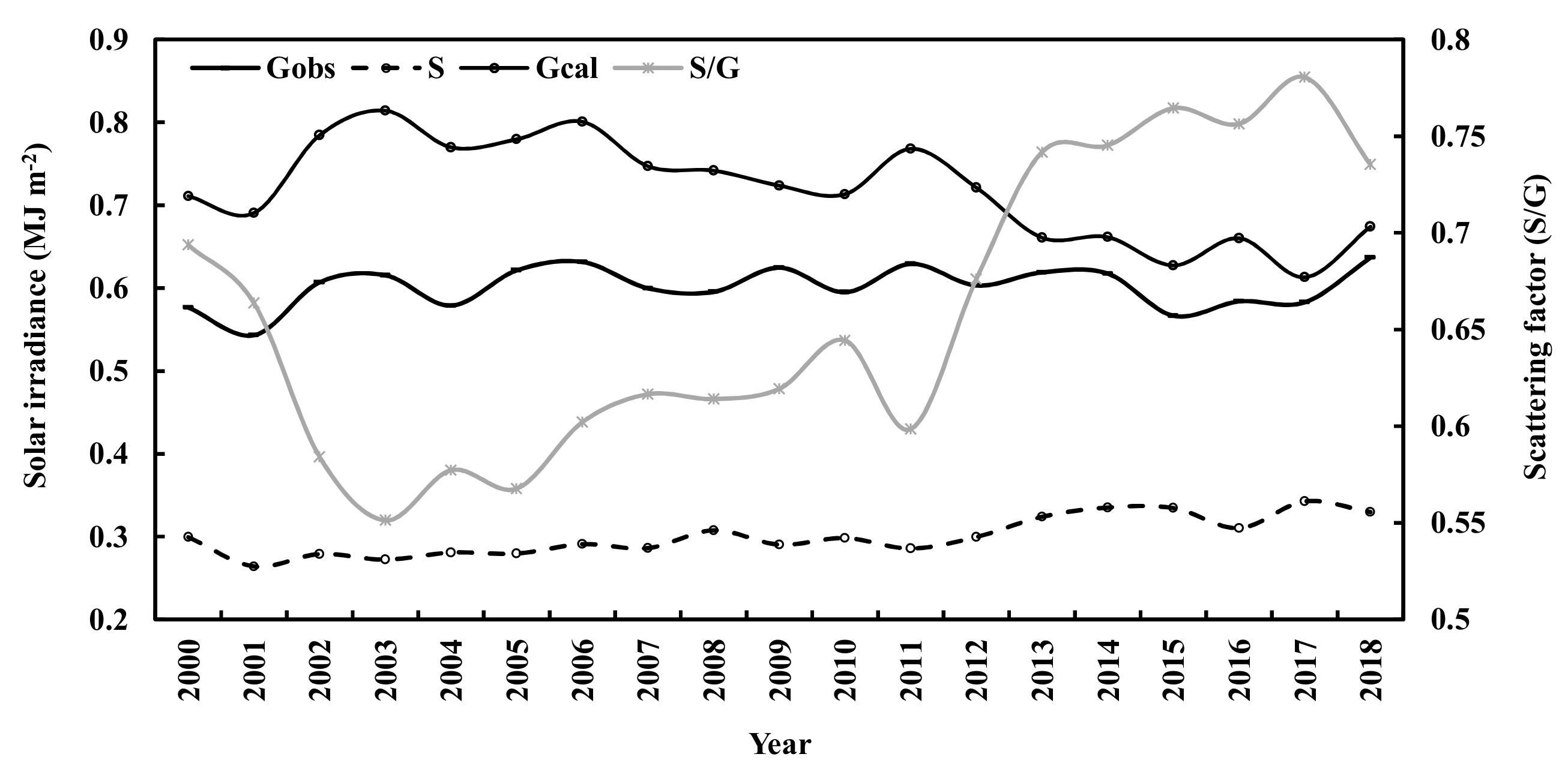
3.1. Global Solar Irradiance during 2000–2018

During 2000–2018, annual averages of observed global and diffuse solar irradiance (n= 92,941) were 0.59 and 0.29 MJ m⁻², thus, the direct horizontal irradiance was a little larger than the diffuse irradiance at the surface, average of S/G was 0.64, and averages of surface air temperature and relative humidity were 0.76 °C (ranged from −39.90 to 31.50 °C) and 80.31%, respectively.

Applying the empirical model of global solar irradiance, hourly global irradiance was calculated for Sodankylä during 1 January 2000 to 31 December, 2018. The input data were observed hourly global and diffuse solar irradiance for S/G and water vapor pressure at the ground. Global solar irradiance in December was too low and not considered in the later analysis, and n decreased to 69,171. The calculated and observed hourly global solar irradiance varied similarly, and calculated values were larger than the observed by 18.11% for the average in 2000–2018. It is reasonable that the empirical model represents the global irradiance and its relationships with absorbing and scattering processes at relative clean atmospheric conditions (i.e., relative low S/G at 0.50 in 2008–2011 in the model development). The calculated and observed monthly global irradiance, diffuse irradiance and S/G are shown in Figure 5. Global solar irradiance in June or July was higher over clean atmospheric conditions, e.g., 2001 to 2003, 2007 and 2011 at low S/G (<0.60), but lower over high GLP loading, e.g., 2008, 2009 and 2017 at high S/G (>0.60). Scattering factor S/G was lower during April to September and higher in October to March.

During 19 years, the monthly averages of the calculated global irradiance decreased by 0.01% and diffuse irradiance increased by 0.11% per year, respectively. They were associated with the increases of S/G by 0.14% and water vapor by 0.06%. Air temperature and relative humidity increased by 0.83% (corresponding to 0.01 °C) and 0.23% for monthly average, respectively. On the average, the annual air temperature increased about 2.09 °C during 2000–2018, also indicating the Arctic warming [27].

Long term interannual variations were also investigated during 2000–2018 (Figure 6 and Figure 7). The calculated annual global solar irradiance decreased by 0.92% and diffuse irradiance increased by 1.28% per year, respectively. Both were associated with the increases of S/G by 1.73% and water vapor by 0.43% per year. Annual air temperature increased by 4.64% (corresponding to 0.07 °C), and relative humidity increased by 0.23% per year, respectively. The annual air temperature showed a higher correlation with water vapor (R = 0.79) than with relative humidity (R = 0.20). A good correlation was determined in annual water vapor pressure (E) and air temperature (T) and relative humidity (RH) as E = 0.293 × T + 0.024 × RH + 3.994 (R = 0.828, n = 19, α = 0.001).

Based on above as well as the following integrated results, the increase of air temperature is evidently associated with the increased GLPs, as well as water vapor. If the output of the Sun remains, solar global radiation at the ground would decrease and air temperature increase with the increase of atmospheric substances in the future.

3.2. The Losses of Global Solar Irradiance in the Atmosphere during 2000–2018

The global solar irradiance losses caused by absorbing and scattering GLPs (G_LA and G_LS) were calculated by using A₁(1-e^−kWm×cos(Z)) and A₂(1-e^−S/G), respectively. The total loss G_L is G_LA + G_LS. The monthly losses due to absorption G_LA dominated the total loss G_L and showed clear seasonal variations, lower in April–September and higher in October–March, whereas G_LS did not have evident seasonal variation and most peaks appeared in October–February. During January 2000 to December, 2018, (1) monthly G_LA decreased slightly by 0.003%, associated with the increase of water vapor by 0.06%; (2) monthly G_LS increased by 0.06%, associated with the increase of S/G by 0.14%; and (3) monthly G_L increased by 0.02% (Figure 8).

For the annual losses of global solar irradiance during 2000–2018, G_LA decreased by 0.02% per year, associating with the increase of E by 0.43%; G_LS increased by 0.72% per year, associating with the increase of S/G by 1.73%; annual G_L increased by 0.24% per year.

The contributions of monthly mean absorbing and scattering losses (R_LA and R_LS) to monthly mean total loss were 63.33% (ranged from 53.95 to 71.99%) and 36.67% (28.01–46.05%), respectively, during January 2000 to December 2018 (Figure 9), corresponding to the monthly averages of water vapor at 6.48 hPa (0.57–14.33) and S/G at 0.55 (0.30–0.94). Generally, R_LA was lower in April–September and higher in October–March, whereas R_LS varied inversely compared to R_LA (i.e., most peaks appeared in October–February). The corresponding annual mean absorbing and scattering losses (R_LA and R_LS) to annual mean total loss were 63.32% (60.09–65.48%) and 36.68% (34.52–39.04%), respectively.

During 2000–2018 at Sodankylä, the annual mean monthly loss of G_LA, G_LS and G_L were 1.94 (1.57–2.41), 1.17 (0.82–1.53) and 3.11 (2.50–3.90) MJ m⁻², corresponding to 539.82, 323.86 and 863.68 W m⁻², respectively.

3.3. Global Solar Irradiance and Its Loss in the Atmosphere from April to September during 2000–2018

To better understand the characteristics of global solar radiation, monthly averages of global solar irradiance and its controlling factors (i.e., E and S/G), meteorological variables, including air temperature, wind speed (v) and square of wind speed, were analyzed, together with their correlations during April–September.

During April–September in 2000–2018, the observed global solar irradiance also decreased a little (0.002%), and the observed diffuse irradiance increased by 0.11%. Air temperature increased by 0.05% (corresponding to 0.010 °C), and relative humidity increased 0.02% for monthly average. The calculated monthly mean global irradiance was larger than the observed by 17.64%, associating with low S/G (0.49) and water vapor pressure (8.83 hPa). The calculated monthly mean global irradiance decreased by 0.07%, corresponding to very little decrease of observed G, which was caused by the increases of S/G by 0.13% and water vapor by 0.03%. The monthly losses G_LA, G_LS and G_L decreased by 0.0002%, 0.078% and 0.029%, respectively, associating with the increases of E and S/G.

The calculated annual global solar irradiance decreased by 0.80% and the observed diffuse irradiance increased by 1.37% per year respectively (Figure 10). Both were associated with the increases of S/G by 1.55% and water vapor by 0.28% per year. Annual air temperature increased by 0.45% (corresponding to 0.04 °C), and relative humidity increased by 0.14% per year, respectively (Figure 11). On the average, the annual air temperature increased 0.78 °C per year during April–September higher than 0.07 °C per year during a whole year in 2000–2018. The annual losses G_LA decreased by 0.01%, associating with the increase of E; G_LS increased by 0.88%, associating with the increase of S/G; total loss G_L increased by 0.32% (Figure 12). G_L showed a similar variation with G_LS, but complicated variation with G_LA. There was a strong correlation between G_L and G_LS (R = 0.99) and a weak correlation between G_L and G_LA (R = −0.07). The contributions of annual mean absorbing and scattering losses (R_LA, R_LS) to annual mean total loss were 63.32% (ranged from 60.96 to 65.48%), 36.68% (34.52–39.04%), respectively, corresponding to the annual averages of water vapor at 8.83 hPa (7.67–9.70) and S/G at 0.49 (0.42–0.60). “Annual mean” air temperature in April–September was 10.14 °C (8.19–11.92). It is evident that G_L was mainly contributed by absorption (G_LA)_, but strongly modulated by scattering (G_LS), indicating the absorbing and scattering GLPs play different roles in the losses of global irradiance.

During April–September, the annual mean loss of G_LA, G_LS and G_L were 1.72 (1.68–1.73), 1.11 and 2.83 MJ m⁻², corresponding to 477.17, 308.33 and 785.50 W m⁻², respectively. These annual mean losses in April–September were less than the corresponding values in a whole year.

Comparing the annual contributions of the energy losses due to absorbing and scattering GLPs, the ratios of R_LA/R_LS were 1.72 and 1.62 for a whole year and for “April–September” at Sodankylä (their averaged S/G were 0.55 and 0.49), and 3.31 and 10.11 for S/G <0.80 and S/G ≥0.80 at Qianyanzhou (refer to as QYZ, a subtropical Pinus forest in China), respectively. It indicates that the high GLP loads results in larger absorbing loss than scattering loss at these two forest regions, i.e., the absorbing substances attenuate much global radiation than scattering substances, especially for QYZ with very high GLP loads.

3.4. Sensitivity Analysis

The response of global solar irradiance to changes of absorbing or scattering substances (i.e., E or S/G) was calculated by using Equation (1) (n = 3962), when another factor kept at its original values. The results are shown in Figure 13 and

Table 2. Changing rates of global solar irradiance (%) caused by the changes of one factor (%), while another factor was kept at its original level.

E (%)								S/G (%)
+20	+40	+80	+160	−20	−40	−80	−100	+20	+40	+80	+160	−20	−40	−80	−100
−1.25	−2.37	−4.30	−7.41	1.44	3.17	8.52	22.08	−10.03	−18.82	−33.37	−53.69	11.45	24.57	56.93	76.86

.

Hourly global solar irradiance at the surface increased/decreased with the decrease/increase of the water vapor, implying that the increased absorbing GLPs result in much loss of global irradiance in the atmosphere and lower irradiance at the surface. Similarly, global solar irradiance increased/decreased with the decreases/increases of the atmospheric scattering GLPs (represented by S/G), indicating that the increased scattering GLPs lead to much loss of global irradiance in the atmosphere. Global solar irradiance was more sensitive to changes in the scattering factor (S/G) than the absorbing factor (E), reflecting that the changes of scattering GLPs (such as aerosols, SOA, clouds) have stronger effects on the global solar radiation than absorbing GLPs, e.g., the mean ratio between the response rate of G to S/G and that to E at different changing rates was about 7.1. The responses of global solar radiation to changes in both E and S/G were negative and nonlinear (Figure 13 and Table 2).

3.5. Estimation and Comparison of Albedos at the TOA and the Surface

Albedos at the TOA and the surface are key factors influencing the energy balance, weather, and climate [28,29,30]. The Clouds and the Earth’s Radiant Energy System (CERES) Energy Balanced and Filled (EBAF) Edition 4.1 [31,32] provides the monthly shortwave flux and incoming solar flux on the TOA for all-sky, clear (for cloud free) sky and clear sky over 1°×1° region (https://ceres.larc.nasa.gov/products.php?product=EBAF-Product accessed on 9 April 2021).

The annual albedos averaged from April to September at the TOA during 2008–2011 were calculated by using the up solar irradiance divided by down solar irradiance and the coefficients in Equation (1):

albedo at the TOA = A₀/(A₁ + A₂)

(2)

The albedo at the surface was calculated by using the following equation:

albedo at the surface = A₀×Atte/(A₁e^−kWm×cos(Z)+ A₂e^−S/G)

(3)

Atte = 1-e^−S/G

(4)

The attenuation rate (Atte) of the scattering term was used to estimate the attenuation of the reflection A₀ at the surface. In general, the albedos at the TOA and the surface obtained from the monthly satellite-retrieved radiance and using Equations (2)–(4) showed similar interannual variations under all skies during 2008–2011 (Supplementary Materials Figure S1). The satellite-retrieved albedos at the TOA (0.414) were larger than those calculated (0.268) with relative bias of 35.26% and absolute error of 0.146 for the 4-year average. The surface downward shortwave irradiance was underestimated by the satellite with mean relative bias of 42.61%, compared to these measured at Sodankylä. So, it was corrected by using the measured monthly shortwave irradiance, and the corrected albedo (0.290) was in closer agreement with the calculated by a smaller relative bias of 7.71% (Supplementary Materials Figure S2).

The calculated and satellite-retrieved annual surface albedos varied similarly with relative bias of 20.00% and absolute error of 0.05 for the 4-year average (Supplementary Materials Figure S1). The calculated and satellite-retrieved annual albedos at the TOA and the surface showed decreasing tendencies during 4 years. Both the calculated and satellite-retrieved albedos showed the similar characteristics, i.e., the albedos at the TOA were larger than the surface.

The above methods were applied to calculate the albedos at the TOA and surface in 2000–2018 (Supplementary Materials Figure S2). During April–September in 2000–2018, the calculated and satellite-retrieved annual albedos at the TOA displayed decreasing trends by 0.58% and 0.07%, respectively, and the corresponding annual albedos at the surface showed increasing trends by 1.24% and 0.10% per year, respectively. As a reference, the atmospheric substances (i.e., S/G) increased by 1.15% per year, water vapor increased by 0.10% per year, and the observed global solar irradiance increased by 0.27% per year during April–September from 2000 to 2018.

To get the accurate albedo, the satellite-retrieved albedo is needed to be corrected by using surface measured global solar irradiance. Considering that the satellite-retrieved upward and downward surface global irradiance was underestimated by 77.58% and 73.99%, respectively, for 2008–2011 and 2000–2018, no corrections were made for satellite-retrieved albedo at the surface. However, this introduced small errors for the albedo comparison. The time and space match is also the main reason for the errors in the comparison. It is reported that the error of the albedo retrieved by MODIS data in the shortwave band is 85.9% [33].

The decrease of albedo at the TOA in 2000–2018 may be caused by (1) the increases of absorbing and scattering GLPs in the atmosphere (represented by E and S/G), including NO₂ (Section 3.8) and absorbing aerosols; (2) the increased emissions of biogenic volatile organic compounds (BVOCs) caused by the increases of air temperature and PAR [34,35], as T and PAR increase with the increase of G simultaneously; (3) the enhanced direct absorption and indirect use of UV and visible radiation by BVOCs and their oxidation products in CPRs reacting with OH radicals [36].

The change of global solar radiation at the ground in 2000–2018 was associated with energy in (1) absorption and scattering caused by all kinds of GLPs in the atmosphere, including gases (CO₂, CH₄, N₂O, NO₂, SO₂, O₃, HCHO, etc.), water vapor, aerosols (black carbon, SOA, etc.), clouds and (2) the reflection by the Earth–atmosphere system at the TOA. All these factors contribute the solar dimming and/or brightening and are suggested to be considered together, not only these commonly recognized gases (e.g., CO₂, CH₄, N₂O, and water vapor), aerosols (e.g., BC), air pollutants and clouds [37,38,39,40,41,42].

The albedos at the TOA and the surface can be obtained from the empirical model in this study (Equations (5)–(7)), as well as obtained from popular radiative transfer models that require more atmospheric inputs, including aerosol, cloud and water properties [43], and not from the current empirical models introduced in the introduction.

3.6. Further Evaluation of the Empirical Model

To evaluate the performance of the empirical model of global solar irradiance under all sky conditions, firstly, the RMSE values were calculated by using the hourly values and were 0.315, 37.70% for 2000–2007 (n = 29,356); 0.353, 45.38% for 2008–2011 (n = 14,525); and 0.329, 42.12% for 2012–2018. These RMSE values were a little larger than that in model development (Section 2.2). It is reasonable, because the measurement errors were larger under these situations. This and other empirical models also show lower performance for cloudy and overcast skies than clear skies [12,13,14,15,16,17,18,19,20,44], indicating that the high atmospheric GLPs (aerosols, clouds, etc.) cause large simulation uncertainties and the model simulation for cloudy sky conditions should be improved in the future.

It also reveals that the RMSE values as well as observation errors decreased with the increase of the observation samples (n). In more detail, the RMSE values were in the range of 0.315 (37.70%) in 2018 to 0.360 (45.12%) in 2005 for each year in 2000–2018. Secondly, the sum of the coefficients (A₁ + A₂ + |A₀|) in Equation (1), the estimated total global irradiance at the TOA, was compared with the solar constant I₀. To further investigate the performance of the empirical model, S/G was divided into different ranges and other parameters (G, S, E, etc.) were also divided with the same ranges as the S/G values. The ratio between the calculated G at the TOA and I₀, relative error between calculated and measured G at the ground, RMSE were calculated and are shown in

Table 3. The ratio between the calculated G at the TOA and I₀, relative error (δavg, δmax) and RMSE (MJ m⁻² and %) between calculated and measured G at the ground.

S/G Range	Ratio	δavg	δmax	RMSE		n
				(MJ m−2)	%
≤0.10	1.232	6.42	29.68	0.031	1.33	137
≤0.20	1.069	8.08	30.51	0.09	4.27	866
≤0.30	0.999	8.6	39.32	0.12	5.78	1322
≤0.40	1.094	9.17	49.22	0.143	7.03	1680
≤0.50	1.145	9.6	51.36	0.16	8.1	2035
≤0.60	1.178	10.19	52.11	0.175	9.18	2371
≤0.70	1.192	10.6	52.37	0.189	10.05	2662
≤0.80	1.216	11.17	52.96	0.198	11.17	3022

.

It provides that the ratio of calculated G at the TOA to I₀ decreased from 1.216 to 0.999 when S/G decreased from S/G ≤ 0.80 to S/G ≤ 0.30, and increased with the S/G further decrease after S/G ≤0.30, i.e., the empirical model can obtain the best simulation of global solar irradiance (ratio = 0.999) under the clean atmospheric condition (S/G ≤0.30), and the sufficient sample number was also an important requirement (n = 1322). As the ratios were increased when S/G continue to decrease from S/G ≤0.20 and the sample numbers were smaller than 1322. Generally, the much clean of the atmosphere, the better simulation of G was manifested. There were relatively large estimation errors (δavg, δmax and RMSE) for the empirical model under high GLP loads (S/G ≥0.50), because the larger errors in measurement and model simulation influenced by aerosols, clouds, rain, fog, etc.

In summary, the simulations of the empirical model were in good agreement with the observations, according to the above performance at the ground and at the TOA.

3.7. Estimation of Aerosol Optical Depth (AOD)

Aerosol optical depth (AOD) from March 2013 to October 2017 was obtained from the Moderate Resolution Imaging Spectroradiometer (MODIS) [45] onboard NASA (National Aeronautics and Space Administration)’s Terra satellite. The daily AOD Dark Target (DT) and Deep Blue (DB) merged L2 product was used to calculate monthly AOD values. The DB algorithm was developed for use over bright surfaces and all land types [46,47,48]. The MODIS/Terra AOD C6.1 data were averaged in a radius of 50 km around the study site [12,49].

The scattering of global solar radiation in the atmosphere is mainly contributed by aerosols, clouds, and water. In a sample way, hourly AOD, hourly mean S/G and water vapor pressure (E) from May 2013 to August 2016 were selected for the following analysis. A strong correlation between S/G and E and AOD was found (R = 0.874, n = 284, α = 0.001), suggesting an empirical equation:

S/G = −0.0027×E + 0.8739 × AOD+ 0.2458

(5)

The statistical metrics were δavg = 6.93% and δmax = 30.76%. Then, this empirical equation was used to calculate AOD, and the δavg = 25.55% and δmax = 56.50%. The standard deviations were 0.07 and 0.08 for satellite-retrieved and calculated AODs, respectively.

To validate the empirical equation for estimating AOD, observational data of solar radiation and water vapor from April 2013 to September 2017 when the satellite AOD values are available were used. The estimated and satellite-retrieved monthly AOD varied in a similar pattern (Supplementary Materials Figure S3), their relative bias ranged from 9.95 to 262.31%, and the maximum of AOD difference was 0.11. Annual mean calculated and satellite-retrieved AODs were also in reasonable agreement with relative bias ranged from 2.92 to 33.39%, and their difference ranged from 0.002 to 0.009 (Supplementary Materials Figure S4). The calculated and satellite-retrieved annual AOD showed similar decreasing trend by 3.48% and 4.93% per year, respectively.

Then, the empirical equation of S/G and AOD was applied to estimate AOD from January 2000 to December 2018, using the observational data at Sodankylä. Monthly AODs from April to September were counted for annual average. Considering the satellite AODs were retrieved usually at low S/G, S/G < 0.45 was used for the S/G criteria. Annual mean AOD showed a low level in 2000–2012, and high level in 2013–2018, their averages were 0.031 and 0.065, respectively, indicating that the AOD was doubled in 2013–2018. From 2000 to 2018, annual mean AOD increased by 8.23% per year (Supplementary Materials Figure S5). The annual S/G from April to September was 0.28 in 2013–2018, and increased by 10.48% compared to 2000–2012 (annual AOD was 0.25). Considering S/G represents the total atmospheric substances (including aerosols, clouds, etc.), it is reasonable that the changing magnitude of AOD was larger than S/G during above two periods.

Atmospheric GLPs, S/G increased by 1.15% per year during 2000–2018. Comparing S/G in January–December, annual mean S/G in 2013–2018 increased by 22.38% compared to 2000–2012, and their annual averages were 0.75 and 0.62, respectively.

The correlation between S/G and E and AOD (R = 0.874) was larger than that between E and AOD (R = 0.523, n = 284), revealing the scattering substance can be mainly separated and expressed as water vapor and aerosols in the atmosphere. The estimated monthly and annual mean AODs varied similarly to the satellite-retrieved AODs. This sample method (Equation (5)) can be used to calculate AOD.

The uncertainties of AOD estimates are mainly from the different time (continuous estimates using Equation (5) and not continuous from the satellite) and space coverage caused by ground and satellite observations, clouds amount in over pass time for the satellite and during a day (i.e., for estimation of AOD without satellite measurement).

To investigate the reason of the increases of the calculated and observed AODs after 2013, we analyzed the monthly averaged total frequent occurrence of seven and three types of aerosols below 12 km derived from the Cloud–Aerosol Lidar and Infrared Pathfinder Satellite Observations (CALIPSO) [50], as well as air temperature in daytime during 2006–2018 (Supplementary Materials Figures S6–S9). The seven aerosol classifications are clean marine, dust, polluted continental/smoke, clean continental, polluted dust, elevated smoke, and dusty marine; and three types of aerosols, namely polluted continental/smoke, clean continental and elevated smoke, were selected to reflect continental and smoke aerosols to some extent.

The averaged AOD in April–September 2014 was higher than in 2013 and in 2015 well corresponding to the frequent occurrences of 3 and 7 type aerosols in August, but, not well with that during April–September (Supplementary Materials Figure S6). Monthly calculated and observed AODs peaked in August, 2014 and other years were in line with the monthly frequent occurrences of 3 and 7 type aerosols (Supplementary Materials Figure S7). The ratios of frequent occurrence of 3 to 7 type aerosols were larger in June, July, August with the average of 0.72, 0.69 and 0.78, and smaller in April, May and September with 0.57, 0.57 and 0.58 during 2007–2018, implying that the important continental and regional aerosol sources, e.g., transportation, smoke and oxidation products of BVOCs. The higher AOD in June–August was well associated with higher air temperature in July–August, together with the larger ratios of 3 to 7 type aerosols, indicating BVOC oxidation and their products in summer play dominant roles in regional aerosol formation. The growth rate of nucleation-mode particles has a clear maximum in summer [51] can be used as evidence.

The averaged wind speeds were 2.42 and 2.47 m s⁻¹, and the south wind was dominated at Sodankylä in each month during April–September in 2002–2012 and 2013–2018. BVOC emissions are mainly driven by air temperature [34,52], their oxidation is an important source of small size aerosols (see References [51,53,54] and references therein), considering the high air temperature usually appears in July, August, especially in 2014 (Supplementary Materials Figures S8 and S9), and the larger contributions of 3 to 7 type aerosols in June, July and August. Taiga forest is the largest terrestrial biological community in the world, covers between 50-degrees latitude north and the Arctic Circle, accounting for 29% of the world’s forest coverage. In addition, biomass burning can lead to increase of BVOC emissions [35]. So, Taiga forest together with biomass burning (e.g., boreal forest fires and agricultural fires) may play important contributions in background aerosol at Sodankylä. The contribution of smoke from the boreal forest and agricultural fires is well documented ([50] and references therein]). The averaged AOD in April–September peaked in 2011, 2014 and 2016, and it also corresponded well to the higher air temperature in July–August. Based on above integrated results, the calculated AOD may be used as a reference to study long-term variations of AOD and SOA production in 2000–2018.

3.8. Estimation of Tropospheric NO₂ Vertical Column Densities

Tropospheric NO₂ vertical column densities (VCDs) from April 2007 to November 2016 were derived from GOME2. The overpass data were calculated for the center of the satellite pixel which includes Sodankylä. The space difference was up to 50 km from the station.

To develop an empirical model for estimation of tropospheric NO₂, observational data of tropospheric NO₂ VCD, global solar radiation and water vapor during April 2008 to November 2011 were selected. Three key processes associated with global solar radiation transfer in the atmosphere were considered:

(1)

Absorption of NO₂ in UV and visible regions: it is expressed by e^−k’cm, k’ is the NO₂ absorption coefficients in UV and visible regions, and 13.01×10⁴ Pa cm⁻¹ [12,55]; c is tropospheric NO₂ VCD (cm⁻²), and m is optical air mass.

(2)

The absorption term: absorption and use of global solar radiation by GLPs, not including NO₂. It is expressed as e^−kWm ×cos(Z). The meaning of this term is discussed in detail in Reference [12].

(3)

The scattering term: scattering of global solar radiation by GLPs is described as e^−S/G.

(4)

This empirical model is a further application of energy balance on a horizontal plane from for O₃ and NO₂ in UV and visible regions to for NO₂ VCD in short wavelength region [12], or empirical model of global solar irradiance, Equation (1).

The hourly global solar irradiance considering NO₂ absorption in all sky conditions was calculated by using the following empirical model:

$$\mathrm{G}={{\mathrm{C}}_1\mathrm{e}}^{-\mathrm{k}’\mathrm{cm}}+{{\mathrm{C}}_2\mathrm{e}}^{-\mathrm{kWm}}\times \cos \left(\mathrm{Z}\right)+{\mathrm{C}}_3{e}^{-\mathrm{S}/{\mathrm{G}}_{\mathrm{obs}}}+{\mathrm{C}}_0$$

(6)

This equation is converted for the estimation of NO₂ VCD, as follows:

$${\mathrm{e}}^{-\mathrm{k}’\mathrm{cm}}={\mathrm{D}}_1\mathrm{G}+{\mathrm{D}}_2\mathrm{e}{-}^{\mathrm{kWm}}\times \cos \left(\mathrm{Z}\right)+{\mathrm{D}}_3{e}^{-\mathrm{S}/{\mathrm{G}}_{\mathrm{obs}}}+{\mathrm{D}}_0$$

(7)

Considering that tropospheric NO₂ VCD was retrieved under low cloud fraction and the solar radiation data with S/G <0.90, NO₂ VCDs within 1 standard deviation were used in the empirical model development (Equation (6)). A strong correlation was found between G and three key terms, the correlation coefficient was 0.956 (n = 216, α = 0.001). The coefficients D_i (i = 1, 2, 3) and the constant D₀ were −0.006, 0.481, 0.006, and 0.639, determined by using a multiparameter fit hourly NO₂ VCD from 8:00 to 19:00 during May 2008–September 2011. The main results are shown in

Table 4. The average and maximum of the absolute relative bias (δavg and δmax (%)), NMSE, and standard deviations of calculated and observed NO₂ VCDs (σcal and σobs, respectively). The mean bias errors (MAD, MJ m⁻² and %) and the root mean square errors (RMSE, MJ m⁻² and %) (n = 216).

δavg	δmax	NMSE	σcal	σobs	MAD		RMSE
					(1015cm−2)	(%)	(1015cm−2)	(%)
13.45	33.23	0.02	0.10	0.12	0.00	0.12	0.09	15.29

. The calculated and observed NO₂ VCDs are presented in Supplementary Materials Figure S9. It is clear that most standard deviations of calculated NO₂ VCDs are less than the satellite derived (Supplementary Materials Figure S9) and similar results is shown in Table 4, σ_cal < σ_obs. In addition, model simulation of annual NO₂ in 2008–2011 was also within 1 standard deviation of the observed in empirical model development (Supplementary Materials Figure S10). It reflects that the reasonable estimations are determined by using the simultaneous NO₂ VCDs in empirical model development.

To validate the empirical model of NO₂ VCD, the tropospheric NO₂ VCD from 8:00 to 19:00 during April 2008 to November 2011 (n = 1445) was calculated by using Equation (7) and the observational data. The calculated NO₂ VCD was underestimated by 47.09% with NMSE =1.76. It is caused by the data-selection criteria in model development, i.e., S/G <0.90 and 1 standard deviation of NO₂ VCD were used. In order to improve the simulation of hourly NO₂ VCD, the constant C₀ was adjusted to 0.535, and the relative bias reduced to −0.99%, NMSE = 0.73 (n = 1445). The relative biases ranged from −0.05 to 10.33% for annual NO₂ VCD in 2008–2011.

Then, these new coefficients were used to estimate tropospheric NO₂ VCDs from 8:00 to 19:00 during April 2000 to November 2018. The annual mean NO₂ VCDs were also obtained from May to October (Supplementary Materials Figure S10). The calculated and satellite-retrieved annual NO₂ VCD increased by 3.83% and 3.23% per year during 2007 to 2016, respectively. Generally, the empirical model displayed a reasonable estimation of hourly NO₂ VCD in annual average and its long-term variation. Tropospheric NO₂ VCD showed a slow increasing trend by 0.03% per year in 2000–2018.

Generally, the estimation of NO₂ VCDs were in agreement with the satellite-retrieved ones for annual average and long-term variation trend during 2007–2017, and the calculated NO₂ VCD had smaller uncertainties than satellite-retrieved values. It should be mentioned that the estimated NO₂ VCDs represent these for the conditions, S/G <0.90, 8:00–19:00 and within 1 standard deviation. The space and time match (continuously obtained from using the Equation (7) and not continuously from the satellite) at ground and satellite observations would introduce estimation errors of NO₂ VCDs. High clouds were not considered in satellite-retrieved NO₂, but it was not for the estimation from using empirical model (i.e., S/G <0.90), especially all NO₂ VCDs analyzed from 8:00 to 19:00. Larger NO₂ VCDs appeared at S/G >0.90 were not used in empirical model development, causing the low annual NO₂ VCD estimations. The satellite observed mean annual NO₂ VCD increased 0.20×10¹⁵ cm⁻² and 16.77% in 2013–2016, compared to that in 2007–2012, it may be caused by biomass burning, well corresponding to the AOD increase in 2013–2017. Some studies report biomass burning (forest fires, deforestation, wildfires, etc.) is a significant source of NOx in global emissions and Amazon forest region [56,57,58].

4. Discussion

4.1. Empirical Model and Estimation of Global Solar Irradiance

An empirical model describing the energy relationships between global solar irradiance and its key processes was developed, based on analyzing representative radiation and meteorological variables measured in natural atmospheric conditions. Global solar radiation is attenuated by absorption and scattering, which are expressed by the absorbing and scattering terms, respectively. It can simulate the global solar irradiance both at the ground and at the TOA, the absorbing and scattering irradiance associated with the GLPs, as well as albedos at the TOA and the surface. This study is to comprehensively investigate the long-term variations of global solar irradiance, the losses of absorbing and scattering energy, albedos at the surface and the TOA, atmospheric constituents (e.g., NO₂ and AOD), and their integrated roles in the Earth–atmosphere system. The empirical model of global solar irradiance is an application of the previous empirical models in the UV, visible and short wavelength bands under all sky conditions [12].

Global solar radiation is attenuated by the atmospheric GLPs, influences the regional vertical and horizontal air movements; for example, the higher the GLP loads, the lower the wind speed. During 2000–2018, wind speed at Sodankylä increased by 0.01% for monthly averages (January–December) and 0.14% for annual averages (Supplementary Materials Figures S11 and S12). The wind speed showed similar variations (e.g., January 2001–August 2001, January 2003–June 2006 and April 2004–October 2004) and opposite variations (e.g., November 2004–January 2005, October 2006–February 2007 and December 2008–June 2009) with the S/G for monthly averages, as well as the similar variations in 2000–2002 and 2012–2018, and opposite variations in 2002–2007 and 2009–2012 for annual averages. In general, GLPs increased by 1.73% per year in 2000–2018.

Supplementary Materials Figure S11 shows the monthly mean wind speed and the monthly mean S/G at Sodankylä during January 2001 to December 2018, and the evident behavior of decreasing wind speed and increasing S/G. Supplementary Materials Figure S13a,b shows monthly wind speed and monthly atmospheric substance for S/G interval at 0.05. These observations reveal that low wind speed associated with the high atmospheric substance loads (S/G). In other words, the increase of atmospheric GLPs, due to direct emission and production from CPRs [59], and transportation from other regions caused much loss of global radiation in the atmosphere, less energy reaching at the surface and long-wavelength radiation heating the atmosphere, and then the decrease of wind speed. Similar phenomenon and mechanism are also displayed at a subtropical region in the northern hemisphere [12].

Global solar radiation arriving at the surface and their absorbing and scattering losses showed obvious monthly and interannual variations (Section 3.3) at this Arctic region, and drives the atmospheric movement on regional scale. It is important to thoroughly investigate radiation transfer, absorbing and scattering processes and their distribution, reflections, and the interactions in radiation—GLPs in the whole atmospheric column.

4.2. Contributions of Absorbing and Scattering

The contribution of absorption (G_LA) to the total loss of global solar irradiance (G_L) was more important than that of scattering (G_LS) (i.e., annual averages of R_LA and R_LS were 63.33% and 36.67% in 2000–2018), meaning that the absorbing substances attenuate more global solar radiation than the scattering substances. In other words, the scattering GLPs play much less important roles in the short wavelength region, compared to the corresponding annual contributions (R_LA and R_LS) of 35.3% and 67.7% in the UV region and 4.7% and 95.3% in the visible region in North China during 2004–2006. The UV radiation excites more GLPs to participate in CPRs, and more energy is consumed in the UV region (35.30%) than in the visible region (4.70%) [36,60]. The similar feature that R_LA is much larger than R_LS is also found in Qianyanzhou subtropical Pinus forest [12], revealing the same mechanism is existed at these two sites. The independence of absorbing and scattering terms in the UV, visible and short wavelength regions helps to describe individual absorbing and scattering process and energy. The absorbing term expresses total absorbing through different mechanisms in the UV, visible and near-infrared regions, and the scattering term expresses the total scattering due to all scattering GLPs [12]. In short, solar radiation in different wavelength regions exhibited different absorbing and scattering characteristics and distributions.

4.3. Long-Term Variations and Interactions in Global Solar Irradiance and Its Losses, Albedos at the TOA and the Surface, NO₂, AOD and S/G

Solar radiation as an important energy input to the Earth–atmosphere system governs and influences air movements, GLP changes and their conversions between gas, liquid and particle phases. All these interactions and dynamic changes between solar energy and GLPs determine the regional climate and climate change.

Compared to the annual averages in 2000–2012, AOD increased double in 2013–2018 (Section 3.7). It was associated with the simultaneous increases of S/G, diffuse radiation and air temperature, and the decrease of global solar radiation. The main reasons are deduced as follows: (1) the increases of local BVOC emissions with the increase of air temperature [34,35], and the further increase of SOA formation from BVOC oxidations [53,54,61,62]; (2) a little increase of tropical NO₂ VCD (1.28%) favorites the chemical and photochemical production of aerosols; (3) long-distance transport of GLPs from the mid-latitude regions, e.g., Southeast Asia [63,64,65]; and (4) much higher S/G at QYZ than at Sodankylä in 2013–2016. Similarly, the annual mean albedo at the surface and NO₂ VCD also increased by 7.58% and 1.28% during January–December in 2013–2018, compared to in 2000–2012, well corresponding to the increases of AOD and S/G. Therefore, all above processes resulted in a small decrease of G (0.69%) and increase of diffuse radiation (22.38%) in 2013–2018, compared to 2000–2012.

It should be discussed about the NO₂ empirical model, the absorption role of NO₂ in the UV and visible regions, its actual energy contribution in solar global radiation is quantified by using the observational data, no matter how small NO₂ is. For example, a similar UV energy balance method is used to simulate surface O₃, considering the relationship in O₃, NO, NO₂, absorbing and scattering term, and UV radiation [66]. The actual roles of O₃, NO and NO₂ are described in a UV balance equation, similar to this study, and surface O₃ variation and the photochemical interactions in O₃ and NO, NO₂ are well revealed; for example, O₃ responses to the changes of NO, NO₂ and water vapor correspond well with the known photochemical mechanisms, reflecting how the signals of NO₂ can be captured and displayed in the empirical model, though NO₂ absorption in the UV region and NO₂ concentration is smaller than O₃. If NO₂ VCDs larger than 1 standard deviation (e.g., 2σ and 3σ) are used in the further development of the empirical model, larger NO₂ VCDs will be captured, especially for these after 2011. In other words, the development of the empirical model depends on the objectives of the investigation.

Based on the above results and other related studies in the mid-latitude and Arctic regions, the comprehensive investigations in the physical, chemical and photochemical, biological processes for the Earth–biosphere–atmosphere system on regional and global scales should be taken into consideration in the future.

4.4. Comparisons of Global Solar Radiation and Its Related Parameters at Two Sites in the Northern Hemisphere

To understand solar global radiation and the interaction between solar global radiation and atmospheric variables in the northern hemisphere, it is benefit to analyze and compare solar global radiation and its loss, other driving factors at two sites in the northern hemisphere. Qianyanzhou, a Pinus plantation at Taihe county, Jiangxi province, China (26°44′48″N, 115°04′13″E), was selected as a representative site in the mid-latitude region. The annual averages of monthly global solar irradiance and other variables were calculated for Sodankylä and QYZ sites (in all sky conditions) during 2013–2016 (

Table 5. Annual averages of monthly global solar irradiance and other variables at Sodankylä (refer to as Sod) and QYZ sites during 2013–2016, and the ratios of all parameters between Sodankylä and QYZ (alb and sur denote albedo and surface, respectively).

Site	Gcal	T	RH	E	S/G	GLA MJm−2	GLS MJm−2	GL	GLA Wm−2	GLS Wm−2	GL	RLA	RLS	alb	alb
	MJm−2	°C	%	hPa				MJm−2			Wm−2	%	%	TOA	sur
Sod	0.65	3.05	76	6.83	0.59	1.94	1.23	3.18	539.65	342.54	882.19	61.96	38.04	0.36	0.22
QYZ	1.42	22.71	75.76	22.38	0.83	1.68	0.27	1.95	466.37	75.35	541.71	89.31	13.69	0.29	0.22
Ratio	0.46	0.13	1	0.3	0.71	1.15	4.56	1.63	1.16	4.55	1.63	0.69	2.77	1.24	0.99

). The ratios of all parameters between Sodankylä and QYZ are also given in Table 5. The calculated global solar irradiance at the surface was 54.23% lower at Sodankylä than QYZ, the total loss of global solar irradiance was 63.08% larger at Sodankylä than QYZ, together with the albedo at the TOA was larger 24.05% at Sodankylä than QYZ, resulting in air temperature was −19.65 °C lower at Sodankylä than at QYZ. The annual averages of E and S/G were much lower at Sodankylä than that at QYZ, but, the longer optical length at Sodankylä than QYZ is a key reason to cause the large losses (G_LA, G_LS, G_L) of global solar irradiance.

Global solar irradiance at the surface decreased at QYZ in 2013–2016, which is mainly caused by the increases of S/G (emissions of GLPs, GLP products from BVOC oxidation and CPRs, etc.) and reflection at the TOA [12]. During 2013–2016, the annual mean loss of G_LA, G_LA and G_L at QYZ were (1) 1.64, 0.49 and 2.13 MJ m⁻² (corresponding to 455.22, 135.50 and 590.72 W m⁻²) for S/G <0.80 conditions, respectively; and (2) 1.69, 0.16 and 1.85 MJ m⁻² for S/G ≥0.80, respectively. These results were obtained by similar calculation as this study, the other information related to BVOCs is reported in Reference [35]. Compared annual averages of Sodankylä during 2000–2018 (Section 3.2) and QYZ during 2013–2016, the ratios of G_LA, G_LS and G_L between Sodankylä to QYZ were 1.18, 2.38 and 1.46, respectively, for S/G <0.80 at QYZ, and 1.15, 7.31 and 1.68, respectively, for S/G ≥0.80 at QYZ. Thus, much global solar radiation, about 46.01% and 68.11%, was attenuated by GLPs higher at Sodankylä than QYZ for these two atmospheric conditions. In addition, more scattered energy was also lost at Sodankylä than QYZ.

The annual contributions of absorbing and scattering losses to annual total loss were 76.77% and 23.23% under the situations of E at 22.11 hPa and S/G at 0.73, and 91.08% and 8.92% under the situations of E at 21.60 hPa and S/G at 0.88 for QYZ. Therefore, affecting factors (i.e., E and S/G) at different levels resulted in the different absorbing and scattering processes and energy lost at two sites. Much global solar energy was scattered in the atmosphere at Sodankylä than QYZ with a factor of 4.55, revealing that the clean atmosphere (lower E and S/G) strongly enhanced the scattering at Sodankylä than QYZ. There were large differences in annual absorbing and scattering losses and their ratios (G_LA/G_LS) were 6.19 at QYZ, and 1.58 at Sodankylä, revealing much more absorbing GLPs than scattering GLPs at these two sites, and this phenomenon/effect was more evident at QYZ than Sodankylä, implying the impacts of their production from regional biogenic and anthropogenic activities.

From 2013 to 2016, the calculated annual albedos at QYZ were 0.242, 0.289, 0.310, 0.323 (0.291, their average, the same hereinafter) at the TOA, and 0.220, 0.211, 0.235, 0.222 (0.222) at the surface. The corresponding values at Sodankylä were 0.356, 0.359, 0.379 and 0.348 (0.361) at the TOA, and 0.222, 0.218, 0.224 and 0.211 (0.219) at the surface. Thus, the calculated albedo at the TOA was larger at Sodankylä than at QYZ, and was similar for the albedo at the surface. The similar annual albedos at the surface were close during 4 years, indicating the reasonable estimations at these two forest regions in the north hemisphere. The larger annual albedo at Sodankylä than at QYZ reveals that the atmospheric substances were more scattering and less absorbing at Sodankylä, conversely, the atmospheric substances were more absorbing at QYZ (Table 4). These differences in the albedo at the TOA are mainly caused by the different regional atmospheric constituents, i.e., cleaner atmosphere at Sodankylä with low water vapor and other GLPs (E and S/G).

Due to much energy was lost in the atmosphere and larger albedo at the TOA at Sodankylä than at QYZ, the annual mean air temperature, 2.35 °C (−23.68 to 21.20 °C), was much lower at Sodankylä (in 2000–2018), compared to the annual mean air temperature, 22.71, 24.94 and 20.77 °C at QYZ for all sky conditions, S/G <0.80 and S/G ≥0.80, respectively (in 2013–2016).

In general, the annual mean ratio of solar absorbing loss divided by S/G and then by air temperature (T) (Q_LA/(S/G)/T) varied slightly at different S/G intervals (S/G < 0.65) during 19 years (Supplementary Materials Figure S14). To decrease the influence of random errors, air temperatures less than one standard deviation and other corresponding variables were removed in the analysis (n = 98). As the sample numbers of monthly ratios of G_LA/(S/G)/T were small (i.e., 1 and 2 for S/G intervals 0.65–0.70 and 0.71–0.75, respectively), and these data were not taken into the calculation. Therefore, averaged ratio (G_LA/(S/G)/T) was 0.32 MJ °C⁻¹ for most representative atmospheric conditions.

Finally, the relationship between G_LA/(S/G) and air temperature (T) was determined at different S/G intervals, and it ranged from 0.30 to 0.75 (R = 0.68, α= 0.05, n = 98):

G_LA/(S/G) = 0.273T + 0.045

(8)

It reveals that the energy of G_LA for the united GLPs is partially converted to thermal energy, which increases the air temperature, and the other part is consumed in photochemical reactions without relation with air temperature, and is a constant (0.045). A relative equilibrium state exited in the interactions between absorbing solar energy divided by atmospheric GLPs and air temperature, using 19-year data, and the increase of absorbing solar energy of 0.273 MJ m⁻² heated the atmospheric GLPs and increased the air temperature by about 1 °C. The calculated absorbing solar energy, thermal and photochemical energy increased with the increases of S/G (Supplementary Materials Figure S15), and their mean averages were 1.79, 1.76 and 0.02 MJ m⁻² (corresponding to 495.70, 489.11 and 6.58 Wm⁻²), respectively. The mean contributions of thermal and photochemical energy to absorbing energy were 98.60% and 1.40%, respectively. The small photochemical energy (ranged from 4.14 to 8.90 W m⁻²) is deduced as UV and visible absorption by all kinds of atmospheric substances.

The total solar absorbing energy (including direct absorption and indirect utilization in UV, visible and near-infrared wavelength regions, such as the known absorbing gases, as well as VOCs, organic compounds, black carbon, etc.) is lost and utilized in the atmosphere should be considered in the study of regional climate and climate change.

Similar to Sodankylä, the relationship between G_LA/(S/G) and air temperature was determined at different S/G intervals at QYZ, and it ranged from 0.70 to 1.00 (n = 40, R = 0.914, α = 0.05):

G_LA/(S/G) = 0.087T + 0.040

(9)

For unite atmospheric GLPs, the increase of absorbing energy of 0.087 MJ m⁻² resulted in the increase of temperature by about 1 °C at QYZ, i.e., which was a factor of 1/3 to that of Sodankylä, and the photochemical energy was 0.040 at QYZ, close to that at Sodankylä. It is clear that much absorbing energy lost in the atmosphere by a factor of 3.14 at Sodankylä than at QYZ results in the large increase of air temperature, and it may be an important reason for the Arctic amplification [1,2,3]. Comparing the annual changing rates (%) in 2000–2018 at Sodankylä and in 2013–2016 at QYZ [12], annual mean S/G increase rate is 1.73% at Sodankylä and 6.08% at QYZ and their ratio is 0.28, whereas annual mean air temperature increases at 2.09 °C for Sodankylä and 0.07 °C for QYZ and their ratio is 28.63, implying that the atmosphere at QYZ has larger total heat capacity than Sodankylä, because of the high atmospheric substances (S/G). Or, the low total heat capacity of the atmosphere at Sodankylä is also benefit to a larger increase in air temperature. Therefore, it is vital to control anthropogenic emissions of GLPs and secondary GLP products through CPRs for controlling regional climate warming.

The calculated absorbing solar energy, thermal and photochemical energy at QYZ also increased with the increase of S/G, and their mean averages were 1.79, 1.76 and 0.03 MJ m⁻² (corresponding to 496.68, 487.70 and 9.00 Wm⁻²), respectively. The mean contributions of thermal and photochemical energy to absorbing energy were 98.17 % and 1.83%, respectively. The photochemical energy was also very low and ranged from 7.19 to 10.82 W m⁻². Similarly, for calculated solar global irradiance (G_cal) at the ground at Sodankylä, the corresponding ratio of G_cal/(S/G)/T decreased with the increase of S/G by 7.66% during 19 years, indicating that no equilibrium state exists in the interaction between solar global radiation at the ground and the GLPs (Supplementary Materials Figure S16).

Similarly, a sensitivity analysis (Supplementary Materials Figure S17) was also performed for QYZ as Sodankylä, using a similar model as Equation (1) and observational data at QYZ [12,35]. At both Sodankylä and QYZ sites, global solar irradiance was more sensitive to the changes in the scattering factor than absorbing factor, and this phenomenon was more prominent at Sodankylä than at QYZ, as the ratio of the response rate to scattering factor to the ratio of the response rate to absorbing factor was 7.10 at Sodankylä and 1.57 at QYZ, indicating that the atmosphere was much more cleaner and drier at Sodankylä than QYZ, as S/G and E were 0.50 and 8.55 at Sodankylä and 0.71 and 23.96 at QYZ, and (S/G)/E was 0.06 at Sodankylä and 0.03 at QYZ. The atmospheric absorbing and scattering GLPs and their changes influence the changes and distributions of global solar radiation at the surface and in the atmosphere (Section 3).

Comparing the responses of G to absorbing and scattering factors between Sodankylä and QYZ, G was more sensitive to changes in the absorbing factor at QYZ than at Sodankylä, which is caused by the higher absorbing GLPs (represented by E, 22.11 hPa) at QYZ than at Sodankylä (E = 8.56 hPa); but, G was more sensitive to changes in the scattering factor at Sodankylä than QYZ, which is associated with the low solar altitude (i.e., long optical length) and low GLPs at Sodankylä (S/G = 0.50) than high solar altitude and high GLPs at QYZ (S/G = 0.73).

5. Conclusions

Solar energy (including global solar radiation and its losses in the atmosphere, the reflection at the TOA and the surface), the atmospheric constituents (including H₂O, gases and aerosols) and their long-term variations are essential to thoroughly understand the physical and chemical processes in the atmosphere, biological processes, and regional climate and climate change at Sodankylä and the Arctic. An empirical model of global solar irradiance (EMGSI) under all sky conditions was developed by using observational data in 2008–2011, at Sodankylä. The calculated hourly global solar irradiance was in agreement with the observed at the ground and the TOA. This model was applied to calculate the global solar irradiance at the ground and its attenuation in the atmosphere from January 2000 to December 2018. The results showed clear monthly and interannual variations. The sensitivity test indicated that global solar irradiance was more sensitive to changes in scattering than absorbing. The responses of global solar irradiance to changes in absorbing and scattering factors were nonlinear and negative. The albedos at the TOA and the surface were calculated by using this empirical model, and the simulated albedos were in agreement with the corresponding satellite-retrieved values.

A good relationship between S/G and AOD was determined and applied to estimate AOD in 2000–2018. An empirical model for estimation of tropospheric NO₂ VCD was developed and used to estimate long-term variations of tropospheric NO₂ VCD in 2000–2018. Negative correlation between the scattering factor and wind speed was found. The enhanced AOD in 2014, especially in August, was probably attributed to Taiga forest and forest fires/biomass burning, i.e., BVOC emissions and BVOC oxidation play important roles in aerosol formation in the Sodankylä region.

During 2000–2018, the estimated global solar irradiance decreased by 0.92%, and diffuse irradiance increased by 1.28% per year. They were associated with the increases of S/G by 1.73% and E by 0.43% per year. Annual air temperature increased by 0.07 °C. Annual mean losses of global solar irradiance in the atmosphere caused by absorbing and scattering GLPs and total loss were 1.94, 1.17 and 3.11 MJ m⁻² (539.82, 323.86 and 863.68 Wm⁻²), respectively. Annual losses of global solar irradiance due to absorbing and scattering substances decreased by 0.02% and increased by 0.72%, respectively, and total loss increased by 0.24% per year. The contributions of annual mean absorbing and scattering losses to total loss were 63.32% and 36.68%, respectively, i.e., more energy was lost in the atmosphere by absorption. The calculated albedos were smaller at the TOA than at the surface. Simulated and satellite-retrieved annual albedos decreased by 0.58% and 0.07% per year at the TOA, and increased by 1.24% and 0.10% per year at the surface, respectively. In 2000–2018, annual mean AOD and tropospheric NO₂ VCD increased by 8.23% and 0.03% per year, respectively.

Global solar radiation and its loss, and other variables at Sodankylä and QYZ in the northern hemisphere were compared. Evident differences were found and were beneficial for our better understanding of the interactions between solar radiation and GLPs, atmospheric movement, regional climate and climate change.

References

1. Cao, Y.F.; Liang, S.L. Recent advances in driving mechanisms of the Arctic amplification: A review. Chin. Sci. Bull. 2018, 63, 2757–2771. (In Chinese) [Google Scholar] [CrossRef] [Green Version]
2. Cohen, J.; Screen, J.A.; Furtado, J.; Barlow, M.; Whittleston, D.; Coumou, D.; Francis, J.A.; Dethloff, K.; Entekhabi, D.; Overland, J.E.; et al. Recent Arctic amplification and extreme mid-latitude weather. Nat. Geosci. 2014, 7, 627–637. [Google Scholar] [CrossRef] [Green Version]
3. Liu, S.Y.; Wang, B.Y.; Xie, Y.X.; Hu, S.H.; Wang, Z.Y.; Yue, L.Y. The Variation Characteristics of Temperature in Barrow Alaska during 1925–2018. Clim. Chang. Res. Lett. 2019, 8, 769–774. [Google Scholar] [CrossRef]
4. Solanki, S.K. Solar variability and climate change: Is there a link. Astron. Geophys. 2002, 43, 5. [Google Scholar] [CrossRef] [Green Version]
5. Elminir, H.K. Relative influence of weather conditions and air pollutants on solar radiation—Part 2: Modification of solar radiation over urban and rural sites. Meteorol. Atmos. Phys. 2007, 96, 257–264. [Google Scholar] [CrossRef]
6. Lean, J.; Rind, D. Climate forcing by changing solar radiation. J. Clim. 1998, 11, 3069–3094. [Google Scholar] [CrossRef]
7. Andreae, M.O.; Ramanathan, V. Climate’s Dark Forcings. Sciences 2013, 340, 280–281. [Google Scholar] [CrossRef] [PubMed]
8. García, R.D.; Cuevas, E.; García, O.E.; Cachorro, V.E.; Pallé, P.; Bustos, J.J.; Romero-Campos, P.M.; de Frutos, A.M. Reconstruction of global solar radiation time series from 1933 to 2013 at the Izaña Atmospheric Observatory. Atmos. Meas. Tech. 2014, 7, 3139–3150. [Google Scholar] [CrossRef] [Green Version]
9. Rosenfeld, D.; Sherwood, S.; Wood, R.; Donner, L. Climate Effects of Aerosol-Cloud Interactions. Sciences 2014, 343, 379–380. [Google Scholar] [CrossRef] [PubMed]
10. Williamson, C.E.; Zepp, R.G.; Lucas, R.M.; Madronich, S.; Austin, A.T.; Ballaré, C.L.; Norval, M.; Sulzberger, B.; Bais, A.F.; McKenzie, R.L.; et al. Solar ultraviolet radiation in a changing climate. Nat. Clim. Chang. 2014, 4, 434–441. [Google Scholar] [CrossRef]
11. Calabrò, E.; Magazù, S. Correlation between Increases of the Annual Global Solar Radiation and the Ground Albedo Solar Radiation due to Desertification—A Possible Factor Contributing to Climatic Change. Climate 2016, 4, 64. [Google Scholar] [CrossRef] [Green Version]
12. Bai, J.H.; Zong, X.M. Global solar radiation transfer and its loss in the atmosphere. Appl. Sci. 2021, 11, 2651. [Google Scholar] [CrossRef]
13. Glover, J.; McCulloch, J.S.G. The empirical relation between solar radiation and hours of sunshine. Q. J. R. Meteorol. Soc. 1958, 84, 172–175. [Google Scholar] [CrossRef]
14. Zhang, J.; Zhao, L.; Deng, S.; Xu, W.; Zhang, Y. A critical review of the models used to estimate solar radiation. Renew. Sustain. Energy Rev. 2017, 70, 314–329. [Google Scholar] [CrossRef]
15. Gueymard, C.A. Critical analysis and performance assessment of clear sky solar irradiance models using theoretical and measured data. Sol. Energy 1993, 51, 121–138. [Google Scholar] [CrossRef]
16. Gueymard, C.A. Clear-sky solar irradiance predictions for large-scale applications using 18 radiative models: Improved validation methodology and detailed performance analysis. Sol. Energy 2012, 86, 2145–2169. [Google Scholar] [CrossRef]
17. Badescu, V.; Gueymard, C.A.; Cheval, S.; Oprea, C.; Baciu, M.; Dumitrescu, A.; Iacobescu, F.; Milos, I.; Rada, C. Accuracy analysis for fifty-four clear-sky solar radiation models using routine hourly global irradiance measurements in Romania. Renew. Energy 2013, 55, 85–103. [Google Scholar] [CrossRef]
18. Bayrakc, H.C.; Demircan, C.; Keceba, A. The development of empirical models for estimating global solar radiation on horizontal surface: A case study. Renew. Sustain. Energy Rev. 2018, 81, 2771–2782. [Google Scholar] [CrossRef]
19. Antonanzas-Torres, F.; Urraca, R.; Polo, J.; Perpinan-Lamigueiro, O.; Escobar, R. Clear sky solar irradiance models: A review of seventy models. Renew. Sustain. Energy Rev. 2019, 107, 374–387. [Google Scholar] [CrossRef]
20. Zang, H.; Cheng, L.; Ding, T.; Cheung, K.W.; Wang, M.; Wei, Z.; Sun, G. Estimation and validation of daily global solar radiation by day of the year-based models for different climates in China. Renew. Energy 2019, 135, 984–1003. [Google Scholar] [CrossRef]
21. Lakkala, K.; Kyro, E.; Turunen, T. Spectral UV Measurements at Sodankylä during 1990–2001. J. Geophys. Res. Atmos. 2003, 108, 4621. [Google Scholar] [CrossRef]
22. Lakkala, K.; Jaros, A.; Aurela, M.; Tuovinen, J.-P.; Kivi, R.; Suokanerva, H.; Karhu, J.; Laurila, T. Radiation measurements at the Pallas-Sodankylä Global Atmosphere Watch station–diurnal and seasonal cycles of ultraviolet, global and photosynthetically—active radiation. Boreal Environ. Res. 2016, 21, 427–444, ISSN 1797-2469. [Google Scholar]
23. Mäkelä, J.S.; Lakkala, K.; Koskela, T.; Karppinen, T.; Karhu, J.; Savastiouk, V.; Suokanerva, H.; Kaurola, J.; Arola, A.; Lindfors, A.; et al. Data flow of spectral UV measurements at Sodankylä and Jokioinen. Geosci. Instrum. Method. Data Syst. 2016, 5, 193–203. [Google Scholar] [CrossRef]
24. Bilbao, J.; Mateos, D.; De Miguel, A. Analysis and cloudiness influence on UV total irradiation. J. Climatol. 2011, 31, 451–460. [Google Scholar]
25. Kondratyev, K.Y.A. Solar Energy; Science Press: Beijing, China, 1962; pp. 123–132. [Google Scholar]
26. Myers, D.R. Solar radiation modeling and measurements for renewable energy applications data and model quality. Energy 2005, 30, 1517–1531. [Google Scholar] [CrossRef]
27. Post, E.; Alley, R.B.; Christensen, T.R.; Macias-Fauria, M.; Forbes, B.; Gooseff, M.N.; Iler, A.; Kerby, J.T.; Laidre, K.L.; Mann, M.E.; et al. The polar regions in a 2 °C warmer world. Sci. Adv. 2019, 5, eaaw9883. [Google Scholar] [CrossRef] [PubMed] [Green Version]
28. Dickinson, R.E. Land surface processes and climate surface albedos and energy balance. Adv. Geophys. 1983, 25, 305–353. [Google Scholar]
29. Li, Z.Q.; Garand, L. Estimation of Surface Albedo from Space: A Parameterization for Global Application. J. Geophys. Res. Atmos. 1994, 99, 8335–8350. [Google Scholar] [CrossRef]
30. Psiloglou, B.E.; Kambezidis, H.D. Estimation of the ground albedo for the Athens area, Greece. J. Atmos. Sol. Terr. Phys. 2009, 71, 943–954. [Google Scholar] [CrossRef]
31. Loeb, N.G.; Doelling, D.R.; Wang, H.; Su, W.; Nguyen, C.; Corbett, J.G.; Liang, L.; Mitrescu, C.; Rose, F.G.; Kato, S. Clouds and the Earth’s Radiant Energy System (CERES) Energy Balanced and Filled (EBAF) Top-of-Atmosphere (TOA) Edition 4.0 Data Product. J. Clim. 2018, 31, 895–918. [Google Scholar] [CrossRef]
32. Kato, S.; Rose, F.G.; Rutan, D.A.; Thorsen, T.J.; Loeb, N.G.; Doelling, D.R.; Huang, X.; Smith, W.L.; Su, W.; Ham, S.H. Surface Irradiances of Edition 4.0 Clouds and the Earth’s Radiant Energy System (CERES) Energy Balanced and Filled (EBAF) Data Product. J. Clim. 2018, 31, 4501–4527. [Google Scholar] [CrossRef]
33. Sun, Y.J.; Wang, Z.H.; Qin, Q.M.; Han, G.H.; Ren, H.Z.; Huang, J.F. Retrieval of surface albedo based on GF-4geostationary satellite image data. J. Remote Sens. 2018, 22, 220–233. [Google Scholar] [CrossRef]
34. Guenther, A.B.; Zimmerman, P.R.; Harley, P.C.; Monson, R.K.; Fall, R. Isoprene and monoterpene emission rate variability: Model evaluations and sensitivity analyses. J. Geophys. Res. Atmos. 1993, 98, 12609–12617. [Google Scholar] [CrossRef] [Green Version]
35. Bai, J.H.; Guenther, A.; Turnipseed, A.; Duhl, T.; Greenberg, J. Seasonal and interannual variations in whole-ecosystem BVOC emissions from a subtropical plantation in China. Atmos. Environ. 2017, 161, 176–190. [Google Scholar] [CrossRef]
36. Bai, J.H. Photosynthetically active radiation loss in the atmosphere in North China. Atmos. Pollut. Res. 2013, 4, 411–419. [Google Scholar] [CrossRef] [Green Version]
37. Shen, Z.B.; Wang, Y.Q.; Wang, W.H.; Wu, J.Z. The attenuation of solar radiation in the polluted urban atmosphere. Plateau Meteorol. 1982, 1, 74–83. [Google Scholar]
38. Wild, M.; Gilgen, H.; Roesch, A.; Ohmura, A.; Long, C.; Dutton, E.; Forgan, B.; Kallis, A.; Russak, V.; Tsvetkov, A. From dimming to brightening: Decadal changes in solar radiation at the Earth’s surface. Science 2005, 308, 847–850. [Google Scholar] [CrossRef] [Green Version]
39. Sweerts, B.; Pfenninger, S.; Yang, S.; Folini, D.; Van Der Zwaan, B.; Wild, M. Estimation of losses in solar energy production from air pollution in China since 1960 using surface radiation data. Nat. Energy 2019, 4, 657–663. [Google Scholar] [CrossRef]
40. Zheng, Z.L.; Zhang, X.L. Long-term variation features of global solar radiation in Beijing. Acta Energ. Sol. Sin. 2013, 34, 1829–1834. (In Chinese) [Google Scholar]
41. Qi, Y.; Fang, S.B.; Zhou, W.Z. Variation and spatial distribution of surface solar radiation in China over recent 50 years. Acta Ecol. Sin. 2014, 34, 7444–7453. (In Chinese) [Google Scholar]
42. Wang, Y.; Wild, M. A new look at solar dimming and brightening in China. Geophys. Res. Lett. 2016, 43, 11777–11785. [Google Scholar] [CrossRef]
43. Valero, F.P.J.; Pope, S.K.; Bush, B.C.; Nguyen, Q.; Marsden, D.; Cess, R.D.; Simpson-Leitner, A.S.; Bucholtz, A.; Udelhofen, P.M. Absorption of solar radiation by the clear and cloudy atmosphere during the Atmospheric Radiation Measurement Enhanced Shortwave Experiments (ARESE) I and II: Observations and models. J. Geophys. Res. Atmos. 2003, 108, 4016. [Google Scholar] [CrossRef]
44. Psiloglou, B.; Kambezidis, H.; Kaskaoutis, D.; Karagiannis, D.; Polo, J. Comparison between MRM simulations, CAMS and PVGIS databases with measured solar radiation components at the Methoni station, Greece. Renew. Energy 2020, 146, 1372–1391. [Google Scholar] [CrossRef]
45. Salomonson, V.V.; Barnes, W.L.; Maymon, P.W.; Montgomery, P.W.; Ostrow, H. MODIS: Advanced facility instrument for studies of the Earth as a system. IEEE Trans. Geosci. Remote Sens. 1989, 27, 145–153. [Google Scholar] [CrossRef]
46. Hsu, N.C.; Tsay, S.C.; King, M.D.; Herman, J.R. Aerosol properties over bright-reflecting source regions. IEEE Trans. Geosci. Remote Sens. 2004, 42, 557–569. [Google Scholar] [CrossRef]
47. Remer, L.A.; Kaufman, Y.J.; Tanré, D.; Mattoo, S.; Chu, D.A.; Martins, J.V.; Li, R.R.; Ichoku, C.; Levy, R.C.; Kleidman, R.G.; et al. The MODIS Aerosol Algorithm, Products, and Validation. J. Atmos. Sci. 2005, 62, 947–973. [Google Scholar] [CrossRef] [Green Version]
48. Sayer, A.M.; Munchak, L.A.; Hsu, N.C.; Levy, R.C.; Bettenhausen, C.; Jeong, M.J. MODIS Collection 6 aerosol products: Comparison between Aqua’s e-Deep Blue, Dark Target, and “merged” data sets, and usage recommendations. J. Geophys. Res. Atmos. 2014, 119, 13965–13989. [Google Scholar] [CrossRef]
49. Sogacheva, L.; de Leeuw, G.; Rodriguez, E.; Kolmonen, P.; Georgoulias, A.K.; Alexandri, G.; Kourtidis, K.; Proestakis, E.; Marinou, E.; Amiridis, V.; et al. Spatial and seasonal variations of aerosols over China from two decades of multi-satellite observations-Part 1: ATSR (1995–2011) and MODIS C6.1 (2000–2017). Atmos. Chem. Phys. 2018, 18, 11389–11407. [Google Scholar] [CrossRef] [Green Version]
50. Kim, M.-H.; Omar, A.H.; Tackett, J.L.; Vaughan, M.A.; Winker, D.M.; Trepte, C.R.; Hu, Y.; Liu, Z.; Poole, L.R.; Pitts, M.C.; et al. The CALIPSO version 4 automated aerosol classification and lidar ratio selection algorithm. Atmos. Meas. Tech. 2018, 11, 6107–6135. [Google Scholar] [CrossRef] [PubMed] [Green Version]
51. Kulmala, M.; Suni, T.; Lehtinen, K.E.J.; Maso, M.D.; Boy, M.; Reissell, A.; Rannik, Ü.; Aalto, P.; Keronen, P.; Hakola, H.; et al. A new feedback mechanism linking forests, aerosols, and climate. Atmos. Chem. Phys. Discuss. 2004, 4, 557–562. [Google Scholar] [CrossRef] [Green Version]
52. Tarvainen, V.; Hakola, H.; Hell’en, H.; Back, J.; Hari, P.; Kulmala, M. Temperature and light dependence of VOC emissions of Scots pine. Atmos. Chem. Phys. Discuss. 2004, 4, 6691–6718. [Google Scholar]
53. Claeys, M.; Graham, B.; Vas, G.; Wang, W.; Vermeylen, R.; Pashynska, V.; Cafmeyer, J.; Guyon, P.; Andreae, M.O.; Artaxo, P.; et al. Formation of Secondary Organic Aerosols Through Photooxidation of Isoprene. Science 2004, 303, 1173–1176. [Google Scholar] [CrossRef] [PubMed] [Green Version]
54. Riccobono, F.; Schobesberger, S.; Scott, C.E.; Dommen, J.; Ortega, I.K.; Rondo, L.; Almeida, J.; Amorim, A.; Bianchi, F.; Breitenlechner, M.; et al. Oxidation Products of Biogenic Emissions Contribute to Nucleation of Atmospheric Particles. Science 2014, 344, 717–721. [Google Scholar] [CrossRef] [Green Version]
55. Schneider, W.; Moortgat, G.K.; Tyndall, G.S.; Burrows, J.P. Absorption cross-sections of NO2 in the UV and visible region (200–700 nm) at 298 K. J. Photochem. Photobiol. A Chem. 1987, 40, 195–217. [Google Scholar] [CrossRef]
56. IPCC (Intergovernmental Panel on Climate Change). Couplings between changes in the climate system and biogeochemistry. In Climate Change 2007: The Physical Science Basis. Contribution of Working Group I to the Fourth Assessment Report of the Intergovernmental Panel on Climate Change; Solomon, S., Qin, D., Manning, M., Chen, Z., Marquis, M., Averyt, K.B., Tignor, M., Miller, H.L., Eds.; Cambridge University Press: Cambridge, MA, USA, 2007; pp. 499–587. [Google Scholar]
57. Potter, C.; Brooks-Genovese, V.; Klooster, S.; Torregrosa, A. Biomass burning emissions of reactive gases estimated from satellite data analysis and ecosystem modeling for the Brazilian Amazon region. J. Geophys. Res. Space Phys. 2002, 107, LBA-23-1–LBA-23-10. [Google Scholar] [CrossRef] [Green Version]
58. Bray, C.D.; Battye, W.H.; Aneja, V.P.; Schlesinger, W.H. Global emissions of NH3, NOx, and N2O from biomass burning and the impact of climate change. J. Air Waste Manag. Assoc. 2021, 71, 102–114. [Google Scholar] [CrossRef]
59. Bai, J.; de Leeuw, G.; De Smedt, I.; Theys, N.; Van Roozendael, M.; Sogacheva, L.; Chai, W. Variations and photochemical transformations of atmospheric constituents in North China. Atmos. Environ. 2018, 189, 213–226. [Google Scholar] [CrossRef]
60. Bai, J.H. UV extinction in the atmosphere and its spatial variation in North China. Atmos. Environ. 2017, 154, 318–330. [Google Scholar] [CrossRef]
61. Jokinen, T.; Berndt, T.; Makkonen, R.; Kerminen, V.-M.; Junninen, H.; Paasonen, P.; Stratmann, F.; Herrmann, H.; Guenther, A.B.; Worsnop, D.R.; et al. Production of extremely low volatile organic compounds from biogenic emissions: Measured yields and atmospheric implications. Proc. Natl. Acad. Sci. USA 2015, 112, 7123–7128. [Google Scholar] [CrossRef] [PubMed] [Green Version]
62. Chu, B.; Kerminen, V.-M.; Bianchi, F.; Yan, C.; Petäjä, T.; Kulmala, M. Atmospheric new particle formation in China. Atmos. Chem. Phys. Discuss. 2019, 19, 115–138. [Google Scholar] [CrossRef] [Green Version]
63. Arnold, S.; Law, K.; Brock, C.; Thomas, J.; Starkweather, S.; Von Salzen, K.; Stohl, A.; Sharma, S.; Lund, M.; Flanner, M.; et al. Arctic air pollution: Challenges and opportunities for the next decade. Elem. Sci. Anth. 2016, 4, 104. [Google Scholar] [CrossRef] [Green Version]
64. Law, K.S.; Stohl, A.; Quinn, P.K.; Brock, C.A.; Burkhart, J.F.; Paris, J.-D.; Ancellet, G.; Singh, H.B.; Roiger, A.; Schlager, H.; et al. Arctic Air Pollution: New Insights from POLARCAT-IPY. Bull. Am. Meteorol. Soc. 2014, 95, 1873–1895. [Google Scholar] [CrossRef] [Green Version]
65. Qiu, J.Y.; Huang, Q.; Tian, W.S.; Xie, F.; Liu, X.R.; Wang, F.Y. Numerical simulation study on the transport of pollution from China to the Arctic region. Plateau Meteorol. 2019, 38, 887–900. [Google Scholar]
66. Bai, J.H. Study on surface O3 chemistry and photochemistry by UV energy conservation. Atmos. Pollut. Res. 2010, 1, 118–127. [Google Scholar] [CrossRef] [Green Version]
Figure 1. Scatter plot of calculated versus observed hourly global solar irradiance from 6:00 to 14:00 during April 2008–August 2011 under all sky conditions at Sodankylä (sample number n = 3962).
Atmosphere 12 00749 g001
Figure 2. Scatter plot of calculated versus observed hourly global solar irradiance from 4:00 to 16:00 during April 2008–August 2011 under all sky conditions at Sodankylä (n = 7442).
Atmosphere 12 00749 g002
Figure 3. The observed and calculated monthly averages of hourly global solar irradiance (Gobs and Gcal) and relative biases (δ) in all sky conditions at Sodankylä.
Atmosphere 12 00749 g003
Figure 4. The observed and calculated annual averages of hourly global solar irradiance (Gobs and Gcal) and relative biases (δ) in all sky conditions at Sodankylä.
Atmosphere 12 00749 g004
Figure 5. Monthly global solar irradiance calculated and observed (G), observed diffuse irradiance (S) and scattering factor (S/G) at Sodankylä.
Atmosphere 12 00749 g005
Figure 6. Annual global solar irradiance calculated and observed (G), observed diffuse irradiance (S) and scattering factor (S/G) at Sodankylä.
Atmosphere 12 00749 g006
Figure 7. Annual air temperature (T), relative humidity (RH) and water vapor pressure (E) at Sodankylä.
Atmosphere 12 00749 g007
Figure 8. Monthly losses of global solar irradiance caused by absorbing and scattering substances (GLA, GLS) and total loss (GL = GLA + GLS) at Sodankylä.
Atmosphere 12 00749 g008
Figure 9. Contributions (RLA, RLS) of monthly absorbing and scattering losses to monthly total loss at Sodankylä.
Atmosphere 12 00749 g009
Figure 10. Annual averages of calculated and observed global solar irradiance, observed diffuse irradiance (S) and scattering factor (S/G) during April–September.
Atmosphere 12 00749 g010
Figure 11. Annual air temperature (T), relative humidity (RH) and water vapor pressure (E) in April–September at Sodankylä.
Atmosphere 12 00749 g011
Figure 12. Annual losses of global solar irradiance caused by absorbing and scattering substances and total loss during April–September. GL uses the right y-axis in the 2 figures.
Atmosphere 12 00749 g012
Figure 13. Changing rates of global solar irradiance (%) caused by the changes of one factor (%), while another factor was kept at its original level.
Atmosphere 12 00749 g013